
E
Four Levels of Models
This appendix provides an illustrative example of four levels of models, running from specific to general, that could be used to support modeling and analysis of the overall system. The outputs of each lower-level model support the higher-level models. An airport landing aide has been selected as the subject of the lowest level model in this example.
Level 1. Assessing the ability of a Local Area Augmentation System (LAAS) to support landings at a particular airport. Characteristic inputs to a Level 1 model of technologies would be LAAS signal structure, the impact of terrain on signal propagation, and the capabilities of aircraft avionics systems (including signal processing and inertial navigation systems). The model’s output would be aircraft position accuracy vis-à-vis the runway and what this would mean for landing the airplane in various weather conditions. Level 1 models can also support detailed analyses of human performance through human-in-the-loop simulations or through detailed agent-based simulations using computational human performance models.
Level 2. Assessing airport landing and takeoff capacity in various weather conditions. LAAS performance would be just one input to this model. Other inputs would include the sequencing of aircraft, how individual aircraft are outfitted, and other automation aides—for example, the Center TRACON Automation System (CTAS) and wake vortex constraints (see Figure E-1). LAAS performance is intended to increase overall airport landing capacity, but the ability to do so is sensitive to runway configuration, the actual weather conditions, aircraft equipage, controller workload, etc. The output of this Level 2 model would characteristically be a set of throughput numbers that are associated with different weather states, although this would obscure the stochastic nature of the model results (see Figure E-2). A Level 2 model might also be used to predict airport congestion. The inputs to such a model would include scheduled arrivals and departures as well as available taxiways and gates. Models of this sort are often used to design and evaluate airport improvements, including new runways and expanded passenger facilities. Figure E-3 shows an example of a model output being used to balance the availability of arrival gates against runway capacity.1
Level 3. Assessing delays across the air transportation system. Inputs include airline schedules (real and projected, based on estimated future demand), airport capacities, aircraft routes between city-pairs, and en route air traffic control sector capacities (see Figure 3-1). The outputs of these models are typically average delays across the entire system, the distribution of such delays by airport, and the mitigation of delays as a function of various changes to the inputs (including airport capacity). The actual model outputs are stochastic, but the stochastic nature of these outputs is often ignored. Other outputs, often ignored, include the delays encountered at specific airports over the course of the day (see Figure E-4). These “ignored” outputs are often important because they help explain the character of the results and the causes for the delays. However, delays at even a single airport may be difficult to calculate; a systemwide model is required to accurately predict traffic levels at an individual airport over the course of a day.
Level 4. Assessing the impact of inadequate air transportation system capacity on the national economy. In contrast to the above models, which were primarily simulations of performance at different levels of detail, this model is prima-
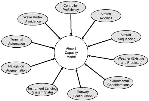
FIGURE E-1 Generic inputs for a model of airport capacity.
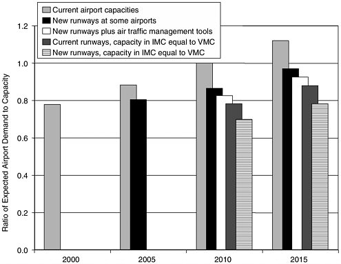
FIGURE E-2 Ratio of expected demand (in terms of landings and takeoffs from an airport) to airport throughput capacity as a function of time (2000 to 2015) and planned airport and terminal area improvements for the 31 largest U.S. airports. IMC, instrument meteorological conditions; VMC, visual meteorological conditions.
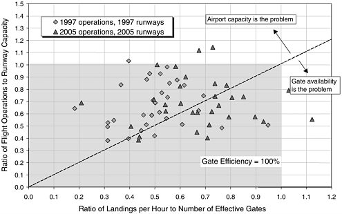
FIGURE E-3 Influence of runway capacity and number of available gates on throughput at the 30 busiest airports in the United States in visual meteorological conditions. Above the dashed line, landing rates are the primary constraint on airport throughput; below the line, gates are the primary constraint.
rily analytic. It has as its inputs the elasticity of passenger (and freight) demand to changes in both ticket price and convenience (essentially another cost to the passenger). Convenience includes frequency of departures to the desired city, the amount of time spent in the airport (which may be driven by aircraft delays as well as security measures at the airport), and the expectation that passengers will actually arrive at their destination without significant delay. This latter concern usually equates to whether a flight will be cancelled or passengers will miss their connections at a hub airport. Also included in such models is an expectation of how the airlines will manage increased demand and the potential for alternative transportation modes that might supplant or complement air travel. Figure E-5 provides an example of the output of such models.
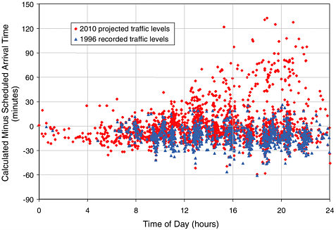
FIGURE E-4 Impact of traffic growth on scheduling predictability at a major U.S. airport in visual meteorological conditions, based on a comparison of scheduled arrival times versus computed arrival times for 1997 (real data) and 2010 (projected data, assuming traffic increases 2.3 percent per year). The large delays occurring in 2010 are not caused by this airport’s planned schedule. The planned arrival rate never exceeds the airport’s acceptance rate, and more planes are not scheduled to arrive at the end of the day than at other times during the day. Delays primarily reflect the accumulated effect of delays at other airports, which result in late arrivals.

FIGURE E-5 Economic losses caused by undercapacity at U.S. airports, assuming that improvements to the air transportation system occur as scheduled.


