
Earthquake Size Estimates and Negative Earthquake Magnitudes
The original and arguably the best-known magnitude scale for measuring the size of an earthquake is the Richter scale, derived by Charles Richter in 1935 at the California Institute of Technology to measure earthquake size in Southern California. Using an early seismograph he defined local magnitude ML to be
ML = LogA – LogAo
where A is the maximum amplitude of deflection of a needle on a chart, in millimeters, measured on the seismograph. Ao is an empirical distance correction appropriate for the region (Richter, 1936). Richter assigned a magnitude 3 to an event with amplitude of 1 mm recorded on a Wood Anderson seismograph at 100 km distance from the source, and a magnitude 0 with amplitude 0.001 mm at 100 km, thought to be the smallest possible instrumentally recorded earthquake (Shemeta, 2010).
Since the 1930s advancements in equipment design such as more sensitive geophones and digital recording equipment and closer proximity to earthquake sources dramatically advanced the ability to record and analyze data from small earthquakes. Using borehole seismic arrays located within a few hundred meters of an earthquake source, very small earthquakes can be recorded. These events are smaller than the baseline magnitude of “0” originally designed by Richter, therefore the range of event sizes continues into the negative magnitude range (Figure E.1).
Because the Richter scale was designed for the Wood Anderson seismograph measurements, its routine use in modern seismology is now quite limited; however, most modern earthquake magnitudes are based on scales that relate back to the Richter scale.
OTHER SIZE ESTIMATES FOR EARTHQUAKES
In practice Richter’s method for estimating earthquake magnitude has been largely supplanted by other more flexible and robust measures of magnitude. The moment magnitude, which is scaled to agree with the Richter magnitude, is in wide use because it can be
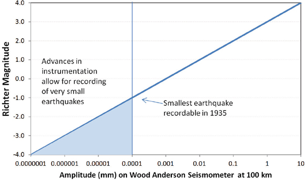
FIGURE E.1 A plot of measured earthquake amplitude versus magnitude. The more sensitive the seismic instruments, the smaller the measureable magnitude, reaching into the negative magnitude range.
tied to other direct measures of the size of an earthquake. The seismic moment is a routine measurement describing the strength of an earthquake and is defined as
Mo = μSd
where μ is the shear modulus, S is the surface area of the fault, and d is the average displacement along the fault. The moment magnitude, Mw, is related to seismic moment by the Hanks and Kanamori (1979) equation
Mw = ![]() LogMo – 6
LogMo – 6
where Mo is in Newton meters, valid for earthquakes ranging from magnitude 3 to 7 (Shemeta, 2010). There are a variety of methods used to calculate a seismic moment from microseismic waveforms.
EARTHQUAKE “B VALUES”
Small earthquakes occur much more often than large earthquakes. The number of earthquakes with respect to magnitude follows a power law distribution and is described by
Log10N = a - bM
where N is the cumulative number of earthquakes with magnitudes equal to or larger than M, and a is the number of events of M = 0. The variable b describes the relationship between the number of large and small events and is the slope of the best-fit line between the number of earthquakes at a given magnitude and the magnitude (Gutenberg and Richter, 1944; Ishimoto and Iida, 1939). A b value close to 1.0 is commonly observed in many parts of the world for tectonic earthquakes. This relationship is often referred to as the Gutenberg-Richter magnitude frequency relationship.
Differences in the slope b reveal information about the potential size and expected number of the events in a population of earthquakes. Analysis of b values around the world has shown that in fluid injection scenarios the b value is often in the range of 2, which reflects a larger number of small events (swarm earthquakes), compared to tectonic earthquakes. In hydraulic fracturing microseismicity, b values in the range of 2 are commonly observed (Maxwell et al., 2008; Urbancic et al., 2010; Wessels et al., 2011). The high b values observed in hydraulic fracturing are thought to represent the opening of numerous small natural fractures during the high-pressure injection (Figure E.2). It is possible for a hydraulic fracture to grow into a nearby fault and reactivate it, if the orientation of the fault is favorable for slip under the current stress conditions in the reservoir. Figure E.3 is an example of a hydraulic fracture reactivating a small fault during injection.
REFERENCES
Gutenberg, B., and C.F. Richter. 1944. Frequency of earthquakes in California. Bulletin of the Seismological Society of America 34:185-188.
Hanks, T.C., and H. Kanamori. 1979. A moment magnitude scale. Journal of Geophysical Research 84(B5):2348-2350.
Ishimoto, M., and K. Iida. 1939. Observations of earthquakes registered with the microseismograph constructed recently. Bulletin of the Earthquake Research Institute 17:443-478.
Maxwell, S.C., J. Shemeta, E. Campbell, and D. Quirk. 2008. Microseismic deformation rate monitoring. Society of Petroleum Engineers (SPE) 116596-MS. SPE Annual Technical Conference and Exhibition, Denver, Colorado, September 21-24.
Richter, C.F. 1936. An instrumental earthquake magnitude scale. Bulletin of the Seismological Society of America 25:1-32.
Shemeta, J. 2010. It’s a matter of size: Magnitude and moment estimates for microseismic data. The Leading Edge 29(3):296.
Urbancic, T., A. Baig, and S. Bowman. 2010. Utilizing b-values and Fractal Dimension for Characterizing Hydraulic Fracture Complexity. GeoCanada—Working with the Earth. ESG Solutions. Available at www.geocanada2010.ca/uploads/abstracts_new/view.php?item_id=976 (accessed April 2012).
Wessels, S.A., A. De La Pena, M. Kratz, S. Williams-Stroud, and T. Jbeili. 2011. Identifying faults and fractures in unconventional reservoirs through microseismic monitoring. First Break 29(7):99-104.
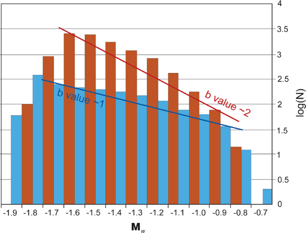
FIGURE E.2 Graph shows b values for two different microearthquake populations during a hydraulic fracture treatment. The b values vary from about 1 for reactivated tectonic microseismic events and 2 for microseismicity associated with the hydraulic fracture injection. The hydraulic fracture microseismic magnitudes are typically very small (less than M 0), hence the lack of larger microseismic events on this b value example. SOURCE: From Wessels et al. (2011).
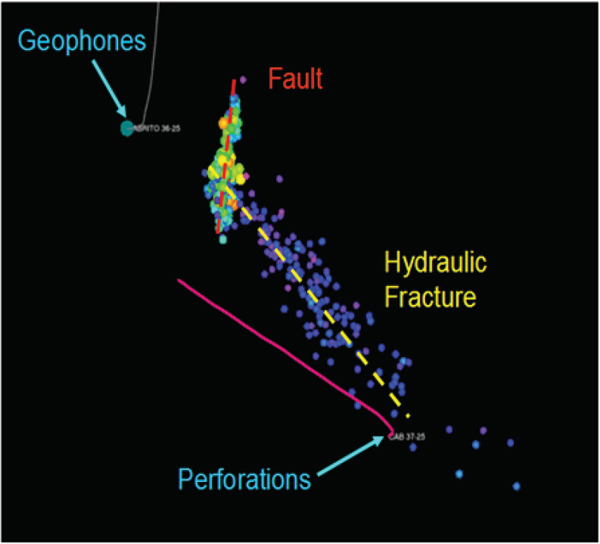
FIGURE E.3 Example of a reactivated fault during hydraulic fracturing. The figure is a map view of a microseismicity (colored spheres which are colored by magnitude; cool colors are small events) during a hydraulic fracture treatment. The fracturing well is shown by the pink line and is deviated away from a central wellhead location and extends vertically through the reservoir section; the injection location is labeled “Perforations.” The data were recorded and analyzed using borehole receivers (marked Geophones). The blue dots show the growth of the hydraulic fracture to the northwest, then intersecting and reactivating a small fault in the reservoir, shown by change in fracture orientation and larger magnitude events (yellow dots). SOURCE: From Maxwell et al. (2008).


