
2
Sources of Uncertainty and Error
The development of a computational model to predict the behavior of a physical system requires a number of choices from both the analyst, who develops the computational model, and the decision maker, who uses model results to inform decisions.1 These choices, informed by expert judgment, mathematical and computational considerations, and budget constraints, as well as aspects of the application at hand, all impact how well the computational model represents reality. Each of these choices has the potential to push the computational model away from reality, impacting the validation assessment and contributing to the resulting prediction uncertainty of the model.
In approaching a system whose performance requires a quantitative prediction, the analyst will typically need to make (or at least consider) a series of choices before the analysis can get under way. In particular, thought needs to be given to the following:
• Relevant or interesting measures of the quantity of interest (QOI) from the point of view of any proposed application or decision;
• The underlying quantitative model or theory to use for representing the physical system;
• The adequacy of that underlying model or theory for the proposed application;
• The degree to which the simulation code, as implemented, approximates the results of the underlying model or theory; and
• The fidelity with which the system is represented in the code.
The last four choices in this list are prime sources of analytic uncertainty. In broad terms, the analyst will be uncertain about (1) the choice of theoretical model to use for predicting the QOI, (2) the inherent adequacy of the theoretical model(s) chosen to predict the QOI, and (3) the degree to which any finite computational implementation of a given model for a given problem approximates the actual model solution for that problem. To proceed to a more fine-grained understanding and taxonomy of sources of analytic uncertainty and error, it will be helpful to consider a specific situation—one that is simplified sufficiently to be tractable and yet complex enough to be
![]()
1 The terms analyst and decision maker refer to the roles that the two parties fulfill. Someone who is a decision maker in one context may well be an analyst in another. For example, scientists are often asked to recommend courses of action with regard to funding research projects. In that role, those scientists will be consumers, rather than producers, of simulation-based information.
relevant to the purposes of this study. Tracing the series of analytic choices above in the context of a particular example should help illustrate where potential areas of analytic uncertainty and error can enter into a representative application of simulation-based prediction.
2.2 PROJECTILE-IMPACT EXAMPLE PROBLEM
Consider the situation depicted in Figure 2.1, which is an example adapted from Thompson (1972). The system under consideration consists of a cylindrical aluminum rod impacting the center of a cylindrical aluminum plate at high speed. This kind of system could be informative when trying to understand the behavior of a projectile impacting armor.
At the start of the problem, the cylindrical rod is moving downward at high velocity and is just touching the thick plate (Figure 2.1, left). The image on the right in Figure 2.1 represents a “slice” through the center of the system and uses color to represent density.
Assume that interest centers on the problem of predicting the behavior of the rod and plate system. First, it must be decided which aspects of the system behavior are required to be predicted—the QOIs. There are several possibilities: the depth of penetration of the plate as a function of impactor velocity, the extent of gross damage to the plate, the fine-scale metallographic structure of the plate after impact, the amount of plate material ejected backward after the rod impact, the time-dependent structure of loading and unloading waves during the impact, and so on. In general, the number of possible QOIs that could be considered as reasonable candidates for prediction is large. Which aspects are important is application-dependent—depending, for example, on whether application focus is on improving the performance of the projectile or of the armor plate—and will influence to a large degree the simulation approach taken by the analyst.
A question that emerges at this stage is the degree of accuracy to which the prediction needs to be made. This also depends on the application under consideration. In this rod and plate example, it may be that the primary QOI
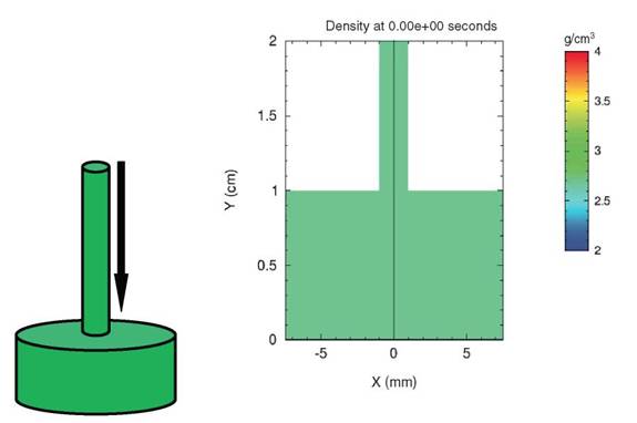
FIGURE 2.1 Aluminum rod impacting a cylindrical aluminum plate.
that is important is the depth of penetration of the rod as a function of impactor velocity, and that the depth only to within a couple of millimeters is the only QOI needed. Having specified the system under consideration, the QOI(s) that require prediction, and the accuracy requirements on that prediction, the analyst can proceed to survey the possible theories or models that are available to estimate the behavior of the system. This aspect of the problem usually requires judgment informed by subject-matter expertise. In this example, the analyst is starting with the equations of solid mechanics. Further, the analyst is assuming that typical impactor velocities are sufficiently large, and the resulting pressures sufficiently high, that the metal rod and plate system can be modeled as a compressible fluid, neglecting considerations of elastic and plastic deformation, material strength, and so on. This is the kind of assumption that draws on relevant background information. Most moderately complex applications rely on such background assumptions (whether or not they are explicitly stated). The specification of the conservation (“governing”) equations is given in Box 2.1. The thermodynamic development is not described in any detail, but the problem of specifying thermodynamic properties requires assumptions about model forms—in this example, shown in Box 2.1. The governing equations and other assumptions combine to determine the mathematical model that will be employed, and the specific assumptions made influence the predicted deformation behavior at a fundamental level. The range of validity of any particular set of assumptions is often far more limited than the range of validity of the governing equations. The subsequent predicted results are bounded by the most limiting range of validity.
At this point, strategies for simulating these equations numerically have to be considered—that is, the computational model must be specified. Accomplishing this is far from obvious, and it is greatly complicated by the existence of nonlinear wave solutions (particularly shock waves) to the equations of fluid mechanics. The details of numerical hydrodynamics will not be explored here, but the important point is that the specification of a well-posed mathematical model to represent the physical system is usually just the beginning of any realistic analysis. Strategies for numerically solving the mathematical model on a computer involve significant approximations affecting the computed QOI. The errors resulting from these approximations may be quantified as part of verification activities. Even after a strategy for solving the nonlinear governing equations numerically is chosen, the thermodynamic relations mentioned above have to be computed somehow. This introduces additional approximations as well as uncertain input parameters, and these introduce further uncertainty into the analysis.
Suppose that both a numerical hydrodynamics code (for addressing the governing equations) and the relevant thermodynamic tables (for addressing the thermodynamic assumptions) are readily available. The next issue to consider is the resolution of the spatial grid to use for discretizing the problem. Finite grid resolution introduces numerical error into the computed solution, which is yet another source of error that contributes to the prediction uncertainty for the QOIs. The uncertainty in the QOIs due to numerical error is studied and quantified in the solution verification phase of the verification, validation, and uncertainty quantification (VVUQ) process. After having made all these choices, the simulation can (finally) be run. The computed result is shown in Figure 2.2.
The code predicts that the rod penetrates to a depth of about 0.7 cm in the plate at the time shown in the simulation. The result also shows strong shock compression of the plate that depends in complicated ways on the location within the plate. Finally, there is evidence of interesting fine-scale structure (due to complex interactions of loading and unloading waves) on the surface of the plate.
Any, or all, of these results may be of interest to both the analyst and the decision maker. The exact solution of the mathematical model cannot be obtained for this problem because the propagation of nonlinear waves through real materials in realistic geometries is generally not solvable analytically. Had the analyst been unable to run the code, he or she might still have been able to give an estimate of the QOI, but that estimate would, most likely, have been vastly more uncertain—and less quantifiable—than an estimate based on a reasonably accurate simulation. A primary goal of a VVUQ effort is to estimate the prediction uncertainty for the QOI, given that some computational tools are available and some experimental measurements of related systems are also available. The experimental measurements permit an assessment of the difference between the computational model and reality, at least under the conditions of the available experiments, a topic that is discussed throughout Chapter 5, “Model Validation and Prediction.” Note that uncertainties in experimental measurements also impact this validation assessment. An important point to realize, for the purposes of this discussion, is that the computational model results all depend on the many choices made in developing the computational model, each potentially pushing the computed QOI away from its counterpart from the true, physical system. Different choices at any of the stages
Box 2.1
Equations for Conservation of Mass, Momentum, and Energy
To be explicit about the form that the rod and plate analysis might take, it is useful to write the governing equations of continuum mechanics. These are laws of conservation of mass, momentum, and energy:1
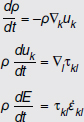
In these equations, ρ denotes the mass density, E the internal energy per unit volume, uk is the velocity vector written in Cartesian coordinates, and ![]() is the stress tensor, again written in Cartesian coordinates.
is the stress tensor, again written in Cartesian coordinates. ![]() denotes the differentiation with respect to the kth spatial direction.
denotes the differentiation with respect to the kth spatial direction.
The strain-rate tensor in the energy equation is given by:
![]()
and the stress tensor in the momentum and energy equations by:
![]()
These equations are quite general and do not depend on assumptions about elastic or plastic deformation, material strength, and the like. They are simply conservation laws, and their introduction is accompanied by very little uncertainty, at least for this application.
However, the specific form taken by the dissipative component of the stress tensor, τdiss, relies on approximations, particularly involving the thermodynamic specification of the system. If, following the analysis mentioned above, it is decided that the rod and plate system will be modeled as a viscous fluid, then the viscous component of the stress tensor can be expressed as a function of the shear and bulk viscosities, ![]() and
and ![]() :
:
![]()
These viscosities (and the internal energy) must be expressed in terms of independent thermodynamic variables, which require approximations that introduce still more uncertainty into the predicted quantities of interest.
_____________________
1 For these equations and notable conventions, see Wallace (1982).
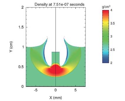
FIGURE 2.2 Aluminum rod at the end of simulation. The figure shows a slice through the system (which began as two cylinders). Color represents density.
discussed above would produce different results from those pictured in Figure 2.2. The results, however, are not equally sensitive to every choice—some choices have greater influence than others on the computational results. A major goal of any uncertainty quantification (UQ) effort is to disentangle these sensitivities for the problem at hand. The problem discussed here exhibits many of the sources of uncertainty that are likely to be present in most computational analyses of physical or engineered systems. It is worthwhile to extract some of the salient themes from this cursory overview.
One uncertainty that the discussion of this example problem did not emphasize is uncertainty in the initial data for the problem. It was simply assumed that the initial dimensions, velocities, densities, and so forth for the combined rod and plate system were known arbitrarily well. Many problems that are commonly simulated do not enjoy this luxury. For example, hydrodynamic simulations of incompressible turbulent flows often suffer from large uncertainties in the initial conditions of the physical system. In principle, these uncertainties must be parameterized in some way and then processed through the simulation code so that different parameter settings describe different initial conditions. If the rest of the modeling process is perfect—something that the above discussion indicates is far from likely—uncertainty in the initial conditions will be the dominant contributor to prediction uncertainty in the QOI. In this case, methods mentioned in Chapter 4, “Emulation, Reduced-Order Modeling, and Forward Propagation,” for the propagation of input uncertainty would describe the prediction uncertainty. The main thrust of the preceding discussion of the example problem has been to point out the many possible additional sources of uncertainty over and above uncertainty in the initial conditions.
Finding: Common practice in uncertainty quantification has been to focus on the propagation of input uncertainties through the computational model in order to quantify the resulting uncertainties in output quantities of interest, with substantially less attention given to other sources of uncertainty.
There is a need for improved theory, methods, and tools for identifying and quantifying uncertainties from sources other than uncertain computational inputs and for aggregating the uncertainties that arise from all sources.
Fidelity of the numerical representation of a complex system is another aspect of many simulation-based predictions that is not well exemplified by the preceding example problem. The geometry of a cylindrical rod impacting a plate is not a particularly difficult geometry to capture in modern computer codes. Many other problems of interest, however, have significant difficulties in capturing all the geometric intricacies of the real system. In many cases, rather complex three-dimensional geometries are simplified to two-, one-, or even zero-dimensional numerical representations.2 But even if the full dimensionality of the problem is retained, it is often the case—especially for intricate systems like a car engine—that many of the pieces of a complex system have to be either ignored or greatly simplified in the code just to get the problem generated or for the code to run stably in a reasonable amount of time.
These decisions are present in most simulation analyses. They are typically made on the basis of expert judgment. One method of determining the effect of a judgment regarding what to neglect or simplify is to try to include a more complete representation and see if it affects the answer significantly. However, if every aspect of the real world could be accurately represented, that is generally what the analyst would do; so in some cases, more detailed modeling is not feasible. An alternative method is to simplify the representation sufficiently that it can be accommodated by the code and computer that are available and accept the impact that the approximate representation has on the simulation output. This is often the only reasonably available strategy for getting an answer and so is frequently the one taken. However, this method also leaves a great deal of latitude to the analyst in making choices on how to represent the system numerically and on judging whether or not the simplifications compromise the simulation results or provide information of utility to the decision maker.
As mentioned briefly in the discussion of the example problem, every analyst confronts the issues of uncertainty in the numerical solution of the equations embodied in the code. Three different broad, but potentially overlapping, categories of uncertainty can be distinguished:
• Inadequate algorithms,
• Inadequate resolution, and
• Code bugs.
Algorithmic inadequacies and resolution inadequacies stem from a common cause: most mathematical models in computational science and engineering are formulated using continuous variables and so have the cardinality of the real numbers; but all computers are finite. In most cases, derivatives are finite differences and integrals are finite sums. Different algorithms for approximating, say, a differential equation on a computer will have different convergence properties as the spatial and temporal resolution are increased. Because the spatial and temporal resolutions or number of Monte Carlo samples of a probability distribution are generally fixed by the computational hardware available, certain algorithms will usually be more appropriate than others. There may be additional factors that also favor one algorithm over another. It is a time-honored warning, though, that every algorithm, no matter how well it performs generally, may have an Achilles’ heel—some weakness that will cause it to stumble when faced with a certain problem. Unfortunately, these weaknesses are usually found in one of two ways: first, by comparing the code against a problem with a known solution; second, by comparing the code against reality. In either case, checks are made to see where the code is found wanting. The problem with checking against a known solution—while undoubtedly a useful and important procedure—is that it is very difficult to determine whether
_____________________
2 An example of a much-used zero-dimensional code is the ORIGEN2 nuclear reactor isotope depletion code. See Croff (1980).
or not the weakness thus revealed in the simple problem will play an important role in the true application. Again, one should note that any judgments made by the analyst on how to factor in algorithmic issues are typically both complex and somewhat subjective.
Resolution inadequacies are slightly different in that they can be checked, at least in principle, by increasing (or decreasing) the spatial and temporal resolutions to estimate the impact of resolution on the simulation result. Notice, again, that here the analyst will be restricted by computational expense and, perhaps, by intrinsic algorithmic limitations.
Finally, code bugs are the rule, not the exception, in all codes of any complexity. Software quality engineering and code verification are finely developed fields in their own right. Nightly regression suites (software to test whether software changes have introduced new errors), manufactured solutions,3 and extensive testing are all attempts to ensure that as many of the lines of code as possible are error-free. It may be trite but is certainly true to say that a single bug may be sufficient to ensure that the best computational model in the world, run on the most capable computing platform, produces results that are utterly worthless.
Finding: The VVUQ process would be enhanced if the methods and tools used for VVUQ and the methods and algorithms in the computer model were designed to work together. To facilitate this, it is important that code developers and model developers learn the basics of VVUQ methodologies and that VVUQ method developers learn the basics of computational science and engineering. The fundamentals of VVUQ, including strengths, weaknesses, and underlying assumptions, are important components in the education of analysts who are responsible for making predictions with quantified uncertainties.
Systems that require computational simulation to predict their evolution in time and space are most frequently intrinsically nonlinear. Fluid dynamics is a paradigmatic example. The hallmark of a nonlinear system is that the dynamics of the system couple many different degrees of freedom. This phenomenon is seen in the example problem of a rod impacting a plate. Steady nonlinear waves, such as shocks, critically depend on the nonlinearity of the dynamical equations. A shock couples the large-scale motions of the solid or fluid system to the small-scale regions where the work done by the viscous stresses is dissipated. Multiscale phenomena always complicate a simulation. As was seen very briefly above, the net effect of the nonlinearity is to present the modeler with a choice of options:
• Option 1: Directly model all the scales of interest, or
• Option 2: Choose a cutoff scale—that is, a scale below which the phenomena will not be represented directly in the simulation, replacing the physical model with another model that is cutoff-dependent.
Each alternative has associated advantages and disadvantages. Option 1 is initially appealing, but it usually dramatically increases the computational expense of even a simple problem, and the time spent in setting up such a simulation might be unwarranted for the task at hand. Moreover, it often introduces additional parameters, governing system behavior at different scales, that need to be calibrated beforehand, frequently in regimes where those parameters are poorly known. The uncertainties induced by these uncertain parameters might exceed the additional fidelity that one could expect from a more complete model. Option 2, on the other hand, reduces the computational expense by limiting the degrees of freedom that the simulation resolves, but it usually involves the construction of physically artificial numerical models whose form is, to some extent, unconstrained and which usually have their own adjustable parameters. In practice, such effective models are almost always tuned, or calibrated, to reproduce the behavior of selected problems for which the correct large-scale behavior is known. The
_____________________
3Manufactured solutions refers to the process of postulating a solution in the form of a function, followed by substituting it into the operator characterizing the mathematical model in order to obtain (domain and boundary) source terms for the model equations. This process then provides an exact solution for a model that is driven by these source terms (Knupp and Salari, 2003; Oden, 1994).
example problem presents the analyst with this choice. In keeping with the usual practice in compressible-fluid numerical hydrodynamics, Option 2 was followed. The dynamics were modeled with an effective numerical model, an artificial viscosity. Each of these options presents its own type of uncertainty.
If it is assumed that the form of the small-scale physics is known (Option 1), then the main residual uncertainty of Option 1 is parametric, that is, due to uncertainty about the correct values to assign to the parameters in the correct physics model. The fortunate aspect of parametric uncertainty is that many methods (e.g., Bayesian, maximum-likelihood) of parameter calibration are available for estimating parameters from experimental data, if such data are available. Again, however, one has to compare the computational expense involved in the direct simulation of many different length scales with the expense of obtaining additional data.
Option 2, choosing a cutoff scale, introduces a potentially important contributor to model discrepancy: model-form uncertainty. When an effective model is created to mimic the physics of the length scales that are deleted from the simulation, the form of the model—the types of terms that enter into the equations—is usually not fully determined by the requirement that the effective model reproduce the physics of a selected subset of large-scale motions. For example, the Von Neumann-Richtmyer artificial viscosity method (Von Neumann and Richtmyer, 1950) (and its descendants) is a way of introducing some effects of viscosity into simulations based on equations that do not otherwise represent the root causes of viscosity. These methods are a good illustration of potential model-form error in that they can accurately propagate planar shocks in a single material—the physics that they are designed to replicate—while failing (in different ways) to model higher-dimensional, or multimaterial, hydrodynamic situations.
A typical strategy to use in constructing effective models is to require that the effective model obey whatever symmetries happen to be present in the full model. In fluid dynamics, for example, one would prefer to have a subgrid model possess the symmetries of the full Navier-Stokes equations.4 Often, however, retaining the full symmetry group is not practicable. Even when it is, however, the symmetry group still usually permits an infinite number of possible terms that may satisfy the symmetry requirements. Which of these terms need to be retained is, unfortunately, often problem-dependent, a fact that can create difficulties for general-purpose codes. Moreover, methods for expressing model-form error, and assessing its impact on prediction uncertainty, are in their infancy compared to methods for addressing parametric uncertainty. Sometimes, however, it is possible to parameterize a model-form uncertainty, allowing it to be treated as a parametric uncertainty. This type of reduction can occur by using parameters to control the appearance of the terms in an effective model after the imposition of symmetry requirements.
The simplified, but still representative, simulation problem discussed here is presented in the hope of identifying at least some sources of error and uncertainty in model-based predictions. It should be clear that the impact of including these different effects is to, on the whole, push a computed QOI away from its counterpart in the physical system, increasing the resulting prediction uncertainty. However, the manner in which this increase occurs will depend considerably on the details of the simulation and uncertainty models under consideration. Some uncertainties will add in an independent manner; others may have strong positive or negative correlations. It is important to realize that some uncertainties may be limited by the availability of relevant experimental data. The most straightforward example occurs when one has data that constrain the possible values of one or more input parameters to the simulation code being used in the analysis. Clearly, the details of such interactions and constraints and the
_____________________
4 These symmetries are discussed in Frisch (1995, Chapter 2).
structure of the analysis are closely interrelated. The sources of uncertainty and error identified here, while almost certainly not an exhaustive list, will likely be present in most simulation-based analyses. Developing quantitative methods to address such a wide variety of uncertainty and error also presents difficult challenges, and exciting research opportunities, to the verification and validation (V&V) and UQ communities.
2.10 CLIMATE-MODELING CASE STUDY
The previous discussion noted that uncertainty is pervasive in models of real-world phenomena, and climate models are no exception. In this case study, the committee is not judging the validity or results of any of the existing climate models, nor is it minimizing the successes of climate modeling. The intent is only to discuss how VVUQ methods in these models can be used to improve the reliability of the predictions that they yield and provide a much more complete picture of this crucial scientific arena.
Climate change is at the forefront of much scientific study and debate today, and UQ should be central to the discussion. To set the stage, one of the early efforts at UQ analysis for a climate model is described (from Stainforth et al., 2005). This study considered two types of input uncertainties for climate models: uncertainty in the initial conditions for the climate model (i.e., the posited initial state of climate on Earth, which is very imprecisely known, particularly with respect to the state of the ocean) and uncertainty in the climate model parameters (i.e., uncertainty in coefficients of equations defining the climate model, related to unknown or incompletely represented physics). It is standard in weather forecasting, and relatively common in climate modeling, to deal with uncertainty in the initial conditions by starting with an ensemble (or set) of possible initial states and propagating this ensemble through the model. It is less common to attempt to deal with the uncertainty in the model parameters, although this has been considered in Forest et al. (2002) and Murphy et al. (2004), for example. The climate model studied was a version of a general circulation model from the United Kingdom Met Office5 consisting of the atmospheric model HadAM36 coupled to a mixed-layer ocean. Out of the many parameters in the model, six parameters—relating to the way clouds and precipitation are represented in the model—were varied over three plausible values (chosen by scientific experts). For emphasis, note that the standard output that one would see from runs of this climate model would be from the run that uses the central value of each of the three possible parameters. Figure 2.3(b) (from Stainforth et al., 2005) indicates the effect of this parameter uncertainty in the prediction of the effect of CO2-doubling on global mean temperature change over a 15-year period. This discussion does not consider the calibration and control phases of the analyses, but note the considerable uncertainty in the final prediction of global mean temperature change at the end of the final CO2-doubling phase. If the climate model were simply run at its usual setting for the parameters, one would obtain only one result, corresponding to an increase of 3.4 degrees. Note also that the initial state of the climate is unknown; to reflect this, a total of 2,578 runs of the climate model were made, varying both the model parameters and the initial conditions. The uncertainty in the final prediction of global mean temperature is then indicated by the larger final spread in Figure 2.3(a).
This discussion only scratches the surface of UQ analysis for climate change. The variation allowed in this study in the model parameters was modest, and only six of the many model parameters were varied. Uncertainty caused by model resolution and incorrect or incomplete structural physics (e.g., the form of the equations) also needs to be considered. The former could be partially addressed by studying models at differing resolutions, and the latter might be approached by comparing different climate models (see, e.g., Smith et al., 2009); it is quite likely, however, that differing climate models make many of the same modeling approximations, and, because of the finite resolution inherent in today’s computers, can only imperfectly resolve difficult topological features. The extent of the effect of chaotic behavior is also poorly understood in climate change (the dust bowl of the 1930s may well have been a chaotic event that would not appear in climate models—see Seager et al., 2009), regional effects are likely to be even more variable, and uncertainty as to future significant changes in forcing parameters (e.g., the actual level of CO2 increase) should also be taken into account. Of course, future CO2 levels depend on human action, which adds more difficulties to an already complex problem.
_____________________
5 See www.metoffice.gov.uk. Accessed August 19, 2011.
6 See Pope et al. (2000).
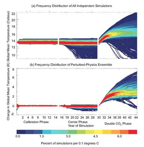
FIGURE 2.3 After calibration and control phases, the effect on global mean temperature of 15 years of doubling of CO2 forcing is considered (a) when both initial conditions and model parameters are varied and (b) when only model parameters are varied. SOURCE: Stainforth et al. (2005).
2.10.1 Is Formal UQ Possible for Truly Complex Models?
The preceding case study provides a useful venue for elaboration on a more general issue concerning UQ that was raised by committee discussions with James McWilliams (University of California, Los Angeles), Leonard Smith (London School of Economics), and Michael Stein (University of Chicago). The general issue is whether formal validation of models of complex systems is actually feasible. This issue is both philosophical and practical and is discussed in greater depth in, for example, McWilliams (2007), Oreskes et al. (1994), and Stainforth et al. (2007). As discussed in this report, carrying out the validation process is feasible for complex systems. It depends on clear definitions of the intended use of the model, the domain of applicability, and specific QOIs. This is discussed further in Chapter 5, “Model Validation and Prediction.”
Several factors make uncertainty quantification for climate models difficult. These include:
1. If the system is hugely complex, the model is, by necessity, only a rough approximation to reality. That this is the case for climate models is indicated by the difficulty of simultaneously tuning climate models to fit numerous outputs; global climate predictions can often be tuned to match various statistics from
nature, but then will be skewed for others. Formally quantifying the uncertainty caused by all of the simplifying assumptions needed to construct a climate model is daunting and involves the participation of people—not just the use of software—because one has to vary the model structure in meaningful ways. One must understand which simplifying assumptions that were made in model construction were rather arbitrary and have plausible alternatives.
Another fundamental challenge is that the resulting variations in model predictions do not naturally arise probabilistically, so that it is unclear how to describe the uncertainty formally and to combine it with the other uncertainties in the problem. For the latter, it might be practically necessary to use a probabilistic representation, but an understanding of the limitations or biases in such an approach is needed.
2. Simultaneously combining all of the sources of uncertainty relating to climate models in order to assess the uncertainty of model predictions is highly challenging, both at the formulation level and in technical implementation.7
3. There is a need to make decisions regarding climate change before a complete UQ analysis will be available. This, of course, is not unique to climate modeling, but is a feature of other problems like stewardship of the nuclear stockpile. This does not mean that UQ can be ignored but rather that decisions need to be made in the face of only partial knowledge of the uncertainties involved. The “science” of these kinds of decisions is still evolving, and the various versions of decision analysis are certainly relevant.
2.10.2 Future Directions for Research and Teaching Involving UQ for Climate Models
In spite of the challenges in the formal implementation of UQ in climate modeling, the committee agrees that understanding uncertainties and trying to assess their impact is a crucial undertaking. Some future directions for research and teaching that the committee views as highly promising are the following:
1. It is important to instill an appreciation that modeling truly complex systems is a lengthy process that cannot proceed without exploring mathematical and computational alternatives. Instead, it is a process of learning the behavior of the system being modeled and understanding limitations in the ability to predict such systems.
2. One must recognize that it is often possible to perform formally UQ only on part of a complex system and that one should develop ways in which this partial UQ can be used. For instance, one might state bounds on the predictive uncertainty arising from the partial UQ and then list the other sources of uncertainty that have not been analyzed. And, as always, the domain of applicability of the UQ analysis must be stated—for example, it may be that the assessment is only valid for predictions on a continental scale and for a horizon of 20 years. This recognition is even more important when one realizes that even a complex system such as a climate model is ultimately itself just a component of a more complex system, involving paleoclimate models, space-time hierarchical models, and so on.
3. There is a tendency among modelers to always use the most complex model available, but such a model can be too expensive to run to allow for UQ analysis. It would be beneficial to instill an appreciation that use of a smaller model, together with UQ analysis, is often superior to a single analysis with the most complex model. In weather forecasting, for instance, it was discovered that running a smaller model with ensembles of initial conditions gave better forecasts than those from a single run of a bigger model. This discovery has carried over to some extent in climate modeling—climate models are kept at a level of complexity wherein an ensemble of initial conditions can be considered, but allowance for UQ with other uncertainties is also needed.
_____________________
7 See, for example, R. Knutti, R. Furer, C. Tebaldi, J. Cermak, and G.A. Mehl. 2010. Challenges in Combining Projections in Multiple Climate Models. Journal of Climate 23(10):2739-2758.
Croff, A.G. 1980. ORIGEN2—A Revised and Updated Version of the Oak Ridge Isotope Generation and Depletion Code. Oak Ridge National Laboratory Report ORNL-5621. Oak Ridge, Tenn.: Oak Ridge National Laboratory.
Forest, C.E., P.H. Stone, A.P. Sokolov, M.R. Allen, and M.D. Webster. 2002. Quantifying Uncertainties in Climate System Properties with the Use of Recent Climate Observations. Science 295(5552):113-117.
Frisch, U. 1995. Turbulence. Cambridge, U.K.: Cambridge University Press.
Knupp, P., and K. Salari. 2003. Verification of Computer Codes in Computational Science and Engineering. Boca Raton, Fla.: Chapman and Hall/CRC.
McWilliams, J.C. 2007. Irreducible Imprecision in Atmospheric and Oceanic Simulations. Proceedings of the National Academy of Sciences 104:8709-8713.
Murphy, J.M., D.M.H. Sexton, D.N. Barnett, G.S. Jones, M.J. Webb, M. Collins, and D.A. Stainforth. 2004. Quantification of Modelling Uncertainties in a Large Ensemble of Climate Change Simulations. Nature 430(7001)768-772.
Oden, J.T. 1994. Error Estimation and Control in Computational Fluid Dynamics. Pp. 1-23 in The Mathematics of Finite Elements and Applications. J.R. Whiteman (Ed.). New York: Wiley.
Oreskes N., K. Shrader-Frechette, and K. Belitz. 1994. Verification, Validation, and Confirmation of Numerical Models in the Earth Sciences. Science 263:641-646.
Pope, V.D., M.L. Gallani, P.R. Rowntree, and R.A. Stratton. 2000. The Impact of New Physical Parameterizations in the Hadley Centre Climate Model: HadAM3. Climate Dynamics 16(2-3):123-146.
Seager, R., Y. Kushnir, M.F. Ting, M. Cane, N. Naik, and J. Miller. 2009. Would Advance Knowledge of 1930s SSTs Have Allowed Prediction of the Dust Bowl Drought? Journal of Climate 22:193-199.
Smith, R., C. Tebaldi, D. Nychka, and L. Mearns. 2009. Bayesian Modeling of Uncertainty in Ensembles of Climate Models. Journal of the American Statistical Association 104:97-116.
Stainforth, D.A., T. Aina, C. Christensen, M. Collins, N. Faull, D.J. Fram, J.A. Kettleborough, S. Knight, A. Martin, J.M. Murphy, C. Piani, D. Sexton, L.A. Smith, R.A. Spicer, A.J. Thorpe, and M.R. Allen. 2005. Uncertainty in Predictions of the Climate Response to Rising Levels of Greenhouse Gases. Nature 433:403-406.
Stainforth, D.A., M.R. Allen, E. Tredger, and L.A. Smith. 2007. Confidence, Uncertainty and Decision-Support Relevance in Climate Predictions. Philosophical Transactions of the Royal Society A: Mathematical, Physical and Engineering Sciences 365(1857):2145-2161.
Thompson, P. 1972. Compressible-Fluid Dynamics. New York: McGraw-Hill.
Von Neumann, J., and R.D. Richtmyer. 1950. A Method for the Numerical Calculation of Hydrodynamic Shocks. Journal of Applied Physics 21(3):232-237.
Wallace, D.C. 1982. Theory of the Shock Process in Dense Fluids. Physical Review A 25(6):3290-3301.


