
Appendix C
Primer on Bayesian Method
The Bayesian approach to statistical inference allows scientists to use prior information about the probability of a given hypothesis or other pieces of a model and to combine it with observed data to arrive at a “posterior”—the probability of the hypothesis given the observed data and our prior information. A simple illustration is HIV testing. Suppose that the hypothesis is about whether John Smith is infected with HIV. And suppose that the evidence is whether a new blood test comes out positive or negative. The abbreviations are as follows:
H = John Smith has HIV
~H = John Smith does not have HIV
E = blood test for John Smith is positive
~E = blood test for John Smith is negative
One wants to determine the probability that John Smith has HIV after receiving the results of a blood test. Suppose that the test is 95% reliable; this means that among those who have HIV, the test will read positive 95% of the time, which can be represented as P(E|H) = 0.95. And suppose that the false-positive rate is tiny (only 1%). That is, among those who do not have HIV, the test will read positive 1% of the time, which can be represented as P(E|~H) = 0.01.
Now suppose that John Smith is routinely screened for HIV with the new blood test and that the test comes back positive. After being informed of the result, he panics because he imagines that he has a 95% or 99% chance of having HIV. That conclusion is not correct. The fundamental theorem, attributed to the Reverend Bayes in the 18th century, is simple in this case to state as follows:
![]()
The equation states that the probability of the hypothesis H given the evidence E (the posterior) is equal to the product of the probability of the evidence E given that H is true (the likelihood) and the probability of H before any evidence (the prior) is provided divided by the probability of E. To avoid computing P(E), scientists sometimes consider the ratio of the posterior of H and ~H, after E is seen, which in this case is as follows:
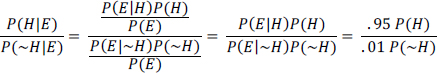
Suppose that, before seeing a blood test, one had no idea whether John Smith had HIV and translated one’s ignorance into a 50-50 probability by saying P(H) = P(~H) = 0.5. Then the ratio
above would equal 95, so P(H|E) = 0.9896, which means that John Smith probably has HIV.1 But suppose that instead of saying that John Smith has a 50% chance of having HIV before one sees a test, one assesses his prior probability of having HIV as the frequency of HIV in people of his age, sex, sexual habits, and drug habits. If John Smith is 30 years old, a middle-class American, heterosexual, and monogamous and does not use any illicit drugs that require needles, his prior might be the frequency of HIV in that group, which might be as low as 1 in 10,000. In this problem, that frequency is referred to as the base rate. If we use P(H) = 0.0001 , the posterior looks much different:
![]()
in which case P(H | E) = 0.0094. Thus, with a base rate of 1 in 10,000, John Smith has less than a 1% chance of having HIV, even though his blood test was positive and the test is a highly reliable one. In that case, the Bayesian approach allows one to incorporate base rates easily and test reliability into a calculation of what one actually cares about: the probability of having HIV after getting a test result.
In more general settings, the Bayesian approach can be used to transfer prior knowledge in one part of a model effectively into posterior knowledge in another part of the model of interest. For example, suppose that the basic causal model of the effect of exposure to lead on a child’s developing brain is as follows:
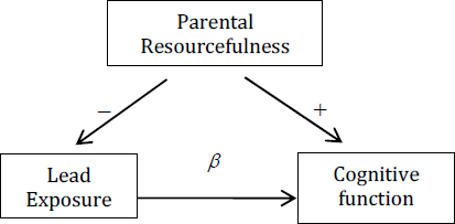
In this model, β, the parameter of interest, represents the size of the effect of lead on cognitive function.2β can be estimated from the observed association between lead exposure and cognitive function after adjusting for parental resourcefulness. One problem, especially if one needs to be able to detect statistically even a fairly small β, is that one must be able to measure parental resourcefulness precisely and reliably.
Suppose that socioeconomic status (SES), such as the mother’s education and income, is used to measure parental resourcefulness.
_____________________________
1This is because P(H|E) + P(~H|E) = 1, and P(H|E)/P(~H|E) = 0.95, which entails that P(H|E) = 0.9896 and P(H|~E)= 0.0104
2Prior beliefs about β can be incorporated directly into a Bayesian model that is used to compute one’s degree of belief about β after seeing data. Prior beliefs about other parts of the model will influence the posterior degree of belief about β indirectly.
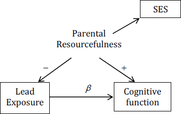
Then the estimate of β will be biased in proportion to how poorly SES measures parental resourcefulness relevant to preventing a child from being exposed to lead and relevant to stimulating the child’s developing brain. The worse SES is as a measure of parental resourcefulness, the more biased the estimate of β. On a scale of 0-100, where 0 means that SES is just random noise and 100 means that it is a perfect measure of parental resourcefulness, is SES a 95? 55? A sensitivity analysis would build a table in which the estimate of β is displayed for each possible level of the quality-of-measure scale of SES, making no judgment about which level is more likely. That can be extremely useful because it might reveal, for example, that as long as one assumes that SES is above a 30 on the quality-of-measure scale, the bias in the estimate of β is below 50%.
Perhaps it is not known where SES sits on a quality-of-measure scale precisely, but one’s best guess is that it is 70, and one is pretty sure that it is between 50 and 90. Then, a Bayesian analysis can incorporate this prior information into a posterior over β. For example, after eliciting information on the amount of measurement error in SES, one can conduct a Bayesian analysis of the size of β that might produce the plot below. The X-axis shows the size of β (which in a simple linear model is the size of the IQ drop that one would expect in a 6-year-old after an exposure to enough lead to increase blood lead by 1 μg/dL), and the Y-axis is the posterior probability of β, given our prior knowledge and the data that have been measured in 6-year-olds.
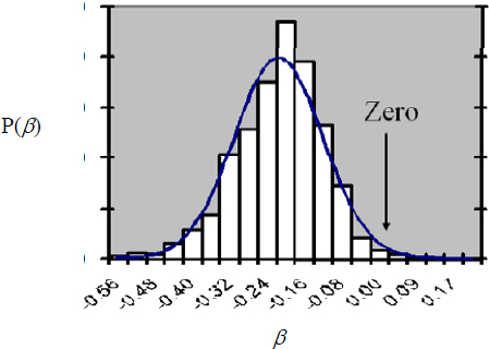
As can be seen, the modal value for β in the posterior is somewhere around -0.2. The spread of the distribution expresses uncertainty about β. Roughly, it shows that the bulk of the posterior distribution over β is roughly between about -0.4 and -0.04. If β is in fact -0.2,
increasing a child’s exposure to lead by an amount that would produce a 20-μg/dL increase in its blood concentration would cause an expected drop in IQ of 4 points.3
In an IRIS assessment, the analogue of β is any parameter that expresses something about the dose-response relationship in humans. Prior knowledge that a Bayesian analysis might incorporate includes
• The degree to which animal data on rodents are relevant to humans.
• The degree to which mechanistic information informs the dose-response relationship in humans.
• The amount of confounding that might still be unmeasured in epidemiologic studies.
• The quality of the measures of exposure in epidemiologic studies.
Although prior elicitation is important for choosing good informative priors, in some situations, particularly if data are sufficient, moderately informative or even noninformative priors might be sufficient. The major danger with Bayesian models for meta-analysis comes with specifying prior distributions for the between-study variance because information for this parameter is limited by the number of studies available and not by the size of each study. Typical noninformative priors do not work well, and some care must be taken to choose one that is sufficiently informative. Enough is often known to establish reasonably loose bounds that enable estimation, although sensitivity analyses that check how much the final answer is affected by prior choice are still necessary.
_____________________________
3Children often test now around 3-5 μg/dL, but children in the 1970s, who were often exposed to lead paint and air with a lot of lead from leaded gasoline, often tested at 20-30 μg/dL.


