
2
DESCRIPTION OF GWEN SYSTEM
The Ground Wave Emergency Network (GWEN) system was designed to protect U.S. communications during a high-altitude nuclear explosion. Such an explosion could affect strategic communications in two important ways. First, the electromagnetic pulse (EMP) produced by a high-altitude nuclear detonation could, over a large area, produce a sudden power surge that would overload unprotected electronic equipment and render it inoperable; in recent years, the Air Force has pursued an extensive program to protect critical electrical components by making them immune to the effects of the EMP-produced power surge. Second, the EMP could interfere with radio transmissions that use the ionosphere for propagation of signals. GWEN uses a ground-hugging wave for propagation, not the ionosphere, and so would be unaffected by high-altitude nuclear detonations. It should be recognized that this ground-hugging wave propagation of the GWEN LF transmitter is no different than that for normal AM radio stations. For the latter sources, the electromagnetic fields also propagate with electric fields that are nearly vertical relative to the ground.
GWEN, developed by the Air Force Electronic Systems Division, calls for three types of stations: input/output stations (I/Os), receive-only stations (ROs), and relay nodes (RNs). I/O stations can both send and receive messages. ROs only receive messages transmitted through I/Os. Unmanned RNs, which would be dispersed throughout the conterminous 48 states, would provide continuous relay links between I/Os and ROs. I/Os and ROs would be at strategic Air Force locations, and RNs would be either on government land or on private land leased by the government. The ground wave used to transmit through the network requires RNs at intervals of approximately 150 - 200 miles.
I/Os would use 50-W transmitters to drive antennae mounted on 20-to 100-ft towers. They would broadcast ultra-high-frequency (UHF) signals in the 224- to 400-MHz band. I/O terminals would enter messages into the RNs by line-of-sight UHF radio links. Airborne I/Os would use the same basic equipment sets and operate at the same power and frequency band as fixed I/Os.
ROs would use 48-in. loop low-frequency (LF) receiving antennae, which would be generally on or near the roofs of existing military communication facilities as would fixed I/Os. Airborne I/Os and portable RO terminals would also use the system. ROs would be installed at fixed locations, and portable units would be stationed at alternate Strategic Air Command (SAC) operating locations. Launch control centers (LCCs) would also be equipped with RO terminals.
Most of the RNs would communicate primarily with other RNs, transmitting with LF antennae at 150 - 175 kHz. Eight of the RNs would receive messages from I/Os
via UHF transmission and transmit messages via the LF antenna to other RNs. All other RNs would have UHF antennae on 60- or 150-ft self-supporting towers for communicating with airborne I/Os.
The overall site area of an RN (see Figure 2-1) would be approximately 11 acres, measuring approximately 700 x 700 feet. A 299-ft-high LF (triangular in cross section, with 2-ft sides) transmitter tower structure with an 8 x 14 x 8-ft antenna-tuning unit (ATU) would be in the center of the site. The structure comprises a concrete foundation 2 ft above grade, a 3-ft-high insulator, a 290-ft steel tower, and 4-ft lightning rods enclosed by a 42 x 47-ft, 8-ft-high chain-link fence topped with barbed wire. The tower itself would be supported by 15 guy wires attached to the ground at six anchor locations. Surrounding the tower and attached to it at the top and anchored in the ground by concrete blocks would be 12 top-loading elements (TLEs). The purpose of the TLEs is to enhance the efficiency of the antenna. Anchors for the TLEs and guy wires would be within the site boundaries.
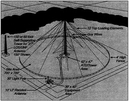
FIGURE 2-1. Proposed layout of typical relay node (RN) station with line-of-sight capability (eight proposed).
A ground plane typically consisting of approximately 100 copper wires, 0.128-in. in diameter (about the thickness of pencil lead) and installed about 12 in. below grade, would radiate approximately 330 ft from the center of the tower. The number (50 -150) and length of copper wires would vary from site to site, depending on soil conductivity. The whole tower area--including guy wires, TLEs, and the ground plane--would be enclosed in a circular 4-ft-high barbed-wire or woven-wire fence. A 30 x 40-ft equipment area enclosed by an 8-ft-high chain-link fence topped with barbed wire would also be on the site. It would be connected to the antenna area by a 10-ft-wide access and service road and to the adjacent road by a 12-ft-wide access and service road.
In addition to the 299-ft LF tower structure, each RN would have a UHF antenna and an LF receiving antenna on a 10-ft mast in the equipment area. The eight RNs within line of sight of the I/Os would have UHF antennae mounted on 60- or 150-ft self-supporting or guyed towers; these towers would be in their own fenced areas enclosed by 8-ft fences topped with barbed wire. The other RNs would have smaller, whip-like UHF antennae mounted on 30-ft light poles within the equipment area. Each RN would have only one type of UHF antenna.
The geographic distribution of GWEN stations is determined by the location of users and the system's technical capabilities. Fixed I/Os and ROs are determined by user needs and would be at existing military facilities. The network configuration of RNs is determined by the necessity to connect fixed and mobile I/Os and ROs and existing thin-line connectivity capability (TLCC) sites. Nominal locations for RNs are derived in part by using a system-wide allocation procedure based on system requirements, predicted signal strength, and ground conductivity. To maintain the required signal strength, actual RN sites should generally be within approximately 9 miles of the nominal locations; the distance will vary with site-specific technical performance factors, such as signal strength and signal-to-noise ratio.
A partial GWEN, called TLCC, is in the construction and testing phase. It contains eight I/Os, 30 ROs, and 56 tower RNs. The FOC phase of GWEN would involve adding four fixed I/Os, 107 fixed ROs, approximately 70 unmanned RNs, 34 airborne I/Os, and a number of portable ROs to the network.
Message injection into the network is by line-of-sight UHF radio links from I/Os to nearby RNs. Message reception via LF RO terminals occurs at key bases throughout the 48 states, including main operating bases of SAC, dispersal bases, and LCCs. I/O and RO terminals are co-located with other manned communications systems at existing military installations; RNs would be unmanned. In addition to transmitting vital messages, the system would be used by SAC and the North American Air Defense Command for exercises and daily status checks among different locations.
The main GWEN antenna would operate intermittently in the LF band at 150 -175 kHz (for comparison, the bottom of the AM band is 530 kHz). The peak broadcasting power would be 2,000 - 3,200 W. The UHF antennae at RNs would operate at 20 W and 225 - 400 MHz. GWEN would not interfere with commercial television or radio broadcasts, amateur radio operations, garage-door openers, or pacemakers.
When broadcasting, the GWEN system would transmit for approximately 2/3 second, receive for 2/3 second, and receive a duplicate message for 2/3 second before repeating the cycle. In its ready status, the GWEN system would nominally make nine 2/3-second transmissions every hour, for a total of 6 seconds/hour. In a 24-hour period, the system would transmit for about 144 seconds or 2.4 min. If the system were to broadcast on a continuous basis for an exercise, it could transmit for a maximum of 6.7 hours in a 24-hour period (but this assumes a level of message input efficiency that does not yet exist).
After discussions with MITRE Corporation staff, we decided to use a duty cycle of 1.4% (0.014 of the time) for our calculations in Chapter 11. This number is probably on the high side but allows for some use of the system in addition to the routine broadcasts (6 seconds/hour) used to check the system.
GWEN will use a procedure called minimum shift keying (MSK). The MSK spectrum, referred to the channel center frequency, has been plotted on a linear scale in Figure 2-2 for the GWEN data rate of 1,200 bits/sec. The actual GWEN signal at the LF carrier frequency consists of intermittent transmissions of packets carrying 644 uncorrelated MSK bits. That is equivalent to a continuous MSK signal turned on and off as packets are transmitted. The resulting “envelope modulation” of the bit stream has an insignificant effect on the normalized signal spectrum of Figure 2-2. There are no spectral lines in the radiated GWEN signal because the uncorrelated bit stream has no periodic components.
During instances of repeated signal transmission, the GWEN signal envelope will appear as a train of pulses of approximately 0.557 second with a pulse repetition period of 2 seconds. The nonlinear process of envelope detection operating on the packet train produces a periodic signal with a DC component, as well as the 0.5-Hz fundamental frequency and its harmonics. Figure 2-3 shows the normalized spectrum of the GWEN packet envelope. The spectral amplitude is related to the radiated signal peak envelope through the proportionality constant At/T, where A is the signal peak envelope, in volts/meter or milligauss; t is the pulse duration; and T is the period. The fraction t/T is the maximum duty cycle of the GWEN LF signal. The DC component is 0.28A, and the fundamental at 0.5 Hz is 0.19A. The 16th harmonic at 8 Hz is more than 20 dB below the fundamental component. The characteristics of the GWEN LF signal and the GWEN transmitter and antenna are summarized in Table 2-1 and Table 2-2.
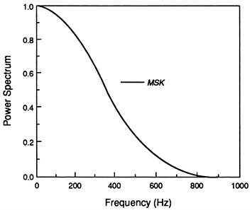
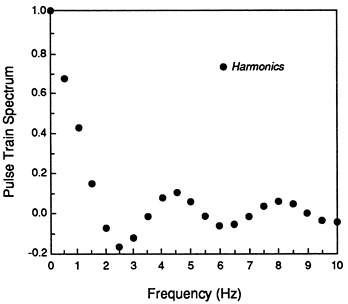
TABLE 2-1. GWEN LF Signal Characteristics
|
Carrier frequency |
150.625-174.625 kHz |
|
Channel spacing |
1, 25 Hz |
|
Number of channels |
20 |
|
Modulation |
Minimum shift keying |
|
Instantaneous data rate |
1,200 bits/sec |
|
Packet length |
644 bits |
|
Packet duration |
537 msec |
|
Minimum transmission interval |
2 sec |
|
Normal message transmission |
3-packet repetition |
|
Average transmitter duty cycle |
0.0017a |
|
aThis number may double to support full implementation of mobile and portable GWEN stations. |
|
TABLE 2-2. GWEN Transmitter and Antenna (Typical Values)
|
Antenna type |
Base-fed, top-loaded monopole |
|
Antenna height |
299 ft |
|
Number of top loading elements |
12 |
|
Ground plane radius |
330 ft |
|
Number of buried copper radial wires |
100 |
|
Input power |
5 kW |
|
Antenna system efficiency |
40-65% |
|
Radiated power |
2-3.2 kW |
The electric field strength depends on the power radiated by the transmitting antenna. GWEN is designed on the basis of a radiated power of 2 kW, so this value has generally been used in estimating exposure. However, some RNs radiate considerably less than 2 kW, and others considerably more. A reasonable upper limit of the power that can be radiated by a GWEN LF antenna is 3.2 kW, and this value is therefore recommended as a “worst case” for estimating exposures.
Two types of geometric dependencies influence electric field strength at a distance. The first is the usual 1/r spreading loss that occurs in the far field of the transmitting antenna as a simple result of the conservation of energy for propagation in a lossless medium. This dependence would be sufficient for describing the geometric effects if the earth were flat. But the 1/r dependence does not apply in the near field of the transmitting antenna. For example, in the case of the electric field strength near a GWEN LF transmitting antenna, the 1/r dependence should be applied only at distances greater than 0.2 mile.
The second dependence is the diffraction loss that results from the earth's being spherical instead of flat. Thus, at longer ranges from the transmitter, a receiving location will be in a geometric shadow zone (i.e., it will be below the horizon). Radiation can then reach the location only through diffraction effects. In the LF range used by GWEN, the shadowing effect reduces electric field strength by less than 1% for ranges less than about 75 miles and by less than 10% for ranges less than about 155 miles. At 300 miles, electric field strength can be reduced by about 35%.
A third influence on electric field strength with increasing distance is absorption loss. The surface of the earth provides a boundary for the propagating electromagnetic wave, and the physical boundary conditions lead to the absorption of energy by the earth. The lower the electrical conductivity of the earth's surface, the larger the loss. That effect leads to losses that are best described in terms of dB per mile. The highest anticipated rate of absorption is about 0.1 dB/mile; this occurs if the effective conductivity of the earth 's surface is 0.5 millisiemen/meter (mS/m), and it reduces the electric field strength by an additional factor (beyond pure geometric effects) of 3 in about 95 miles and by a factor of 10 in 200 miles. But, there are portions of the United States where the effective conductivity is 30 mS/m; in this case, the rate of absorption is only 0.0042 dB/mile, which leads to an additional reduction (beyond pure geometric effects) by only 5% in 200 miles.
Figure 2-4 shows the relationship between distance and the electric and magnetic field strengths for the LF transmitter. Figure 2-5 is a similar diagram showing electric field strength vs. distance for the UHF transmitter. The contribution of the UHF antenna is much smaller than that of the LF transmitter. Detailed survey data around
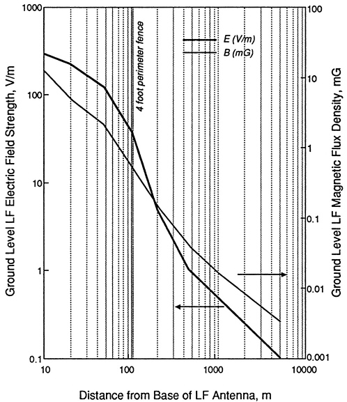

candidate sites do not exist. However, because most candidate GWEN sites are relatively remote, the background levels are not expected to be high enough that the addition of the GWEN fields is going to push levels above the accepted guidelines for public exposure (see Chapter 10).
Populations around 40 proposed GWEN RN sites have been estimated by examining U.S. Geological Survey maps of randomly chosen candidate locations for each site. All structures, unless specifically identified otherwise, were counted as homes. Structures were counted in each of six contiguous concentric zones with outer boundaries of 0.2, 0.3, and 0.5, 1, 2, and 4 km. A value of 2.6 persons/structure was used to estimate populations. Table 2-3 summarizes the data for these 40 sites and presents calculations of minimum and maximum E and B fields encountered in each zone. Population densities are low; it is estimated that approximately 800 people would reside within 1 km of the antenna. LF fields at the 1-km boundary are estimated to be 0.54 to 1.0 V/m for the E field and 1.8 to 4.2 µG for the B field. For comparison, it has been estimated that in 15 metropolitan areas surveyed by the U.S. Environmental Protection Agency about 1.3 million people would be exposed to E-fields of more than 1.0 V/m.
TABLE 2-3. Numbers of Houses Within Six Contiguous Concentric Zones Around 40 RN Sites. Dmin is Distance from Center of Site to Nearest House.
|
Region |
||||||||
|
Site |
1 |
2 |
3 |
4 |
5 |
6 |
D min. ft |
|
|
<200 m |
200-300 m |
300-500 m |
5-1 km |
1-2 km |
2-4 km |
|||
|
901 |
0 |
1 |
0 |
2 |
6 |
46 |
1000 |
|
|
902 |
1 |
1 |
0 |
5 |
11 |
69 |
500 |
|
|
903 |
1 |
0 |
3 |
4 |
37 |
310 |
625 |
|
|
904 |
1 |
0 |
0 |
3 |
28 |
152 |
500 |
|
|
905 |
0 |
0 |
2 |
13 |
40 |
235 |
1125 |
|
|
906 |
1 |
1 |
1 |
7 |
18 |
75 |
600 |
|
|
907 |
3 |
2 |
9 |
17 |
57 |
139 |
375 |
|
|
908 |
0 |
0 |
2 |
12 |
78 |
195 |
1250 |
|
|
909 |
0 |
0 |
4 |
27 |
22 |
123 |
1000 |
|
|
910 |
0 |
0 |
1 |
6 |
45 |
66 |
1250 |
|
|
911 |
0 |
0 |
0 |
0 |
0 |
365 |
9000 |
|
|
912 |
0 |
0 |
2 |
3 |
33 |
42 |
1125 |
|
|
913 |
0 |
0 |
0 |
1 |
0 |
7 |
1750 |
|
|
914 |
0 |
0 |
0 |
3 |
12 |
115 |
2000 |
|
|
915 |
0 |
0 |
0 |
1 |
30 |
51 |
2400 |
|
|
916 |
0 |
0 |
0 |
2 |
2 |
6 |
2375 |
|
|
917 |
0 |
0 |
1 |
0 |
0 |
1 |
1000 |
|
|
918 |
0 |
0 |
0 |
0 |
0 |
13 |
11500 |
|
|
919 |
0 |
0 |
0 |
0 |
2 |
20 |
2001 |
|
|
920 |
0 |
0 |
0 |
0 |
1 |
4 |
6250 |
|
|
921 |
0 |
0 |
0 |
0 |
0 |
0 |
13120 |
|
|
922 |
0 |
0 |
0 |
0 |
0 |
15 |
10250 |
|
|
923 |
0 |
0 |
0 |
2 |
10 |
15 |
2250 |
|
|
924 |
1 |
0 |
2 |
0 |
2 |
1 |
375 |
|
|
925 |
0 |
0 |
0 |
5 |
55 |
417 |
2200 |
|
|
926 |
2 |
0 |
0 |
6 |
20 |
51 |
1000 |
|
|
927 |
0 |
2 |
2 |
5 |
11 |
19 |
875 |
|
|
928 |
1 |
0 |
0 |
2 |
6 |
12 |
440 |
|
|
929 |
1 |
0 |
0 |
0 |
1 |
3 |
435 |
|
|
930 |
1 |
0 |
0 |
1 |
5 |
11 |
500 |
|
|
931 |
0 |
0 |
0 |
0 |
3 |
5 |
3400 |
|
|
932 |
0 |
0 |
0 |
1 |
4 |
18 |
2400 |
|
|
933 |
0 |
0 |
1 |
13 |
28 |
110 |
1040 |
|
|
934 |
0 |
0 |
1 |
1 |
10 |
23 |
2000 |
|
|
935 |
0 |
0 |
0 |
3 |
11 |
32 |
1625 |
|
|
936 |
0 |
0 |
0 |
4 |
15 |
52 |
2750 |
|
|
937 |
0 |
1 |
2 |
11 |
42 |
90 |
625 |
|
|
938 |
0 |
2 |
3 |
7 |
70 |
285 |
750 |
|
|
939 |
0 |
0 |
0 |
0 |
15 |
355 |
5250 |
|
|
940 |
0 |
3 |
2 |
18 |
57 |
79 |
625 |
|
|
AVG |
0.325 |
0.325 |
0.95 |
4.625 |
19.675 |
90.675 |
2488.4 |
|
|
ST DEV |
0.647592 |
0.7206768 |
1.6725729 |
5.965264 |
21.11799 |
112.0539 |
3115.651 |
|
|
SUM |
13 |
13 |
38 |
185 |
787 |
3627 |
||
|
CUM SUM |
13 |
26 |
64 |
249 |
1036 |
4663 |
||
|
Area, km2 |
0.0801 |
0.237 |
0.7399 |
3.096 |
12.52 |
50.2 |
||
|
Avg Density (houses/km2) |
4.06 |
1.37 |
1.28 |
1.49 |
1.57 |
1.81 |
||


