
3
Scientific Background: Earth Exploration Satellite Service
The Earth Exploration Satellite Service (EESS) is dedicated to monitoring and studying phenomena that affect habitat of our planet Earth and its environmental quality. These services use spaceborne active and/or passive microwave sensors to provide valuable measurements of atmosphere, land, and sea, for both research and operational purposes. Because all matter emits, absorbs, and scatters electromagnetic energy to varying degrees, these sensors detect variations in Earth’s environment. Spaceborne sensors operating at radio frequencies (RF) can detect these variations under all weather conditions because of their longer wavelengths, and with penetration depths not possible at optical or infrared wavelengths. RF used for EESS are usually designated either as “windows” used for observing Earth’s surface or as “opaque” used for observing the atmosphere (Figure 3.1). However, it should be noted that all window channels exhibit some atmospheric absorption and emission, and even atmospheric resonant frequencies or absorption bands are often not completely opaque. Hence, most sensors incorporate both window and opaque channels.
Spaceborne sensors can monitor environmental conditions repetitively on a global scale. They measure temperature, humidity, cloud, and trace gas profiles in the atmosphere; moisture, roughness, and biomass at the land surface; salinity, temperature, surface wave height, and sea state in the oceans; and water content and melt character of ice and snow. These measurements are critical to predicting and monitoring of weather and severe storms; managing water resources, land, and biota; and understanding changes in global climate and atmospheric chemistry. As mentioned in Section 1.6, the long-term economic impact of the information from remote sensing satellites is substantial, in both the production of food and other agricultural products and in the operation of businesses and industries that are dependent on knowledge of local weather and changes in climate. Each year many thousands of lives are saved, globally, through advance warning of dangerously inclement weather, for example, hurricanes, tornadoes, severe thunderstorms, flash floods, and droughts.
In addition to using spectrum for spaceborne active and passive sensing, the Earth science services use spectrum for command, tracking, data acquisition, and communications and for ground-based radiometry of the atmosphere (see Section 1.5). Ground-based passive and active microwave sensors
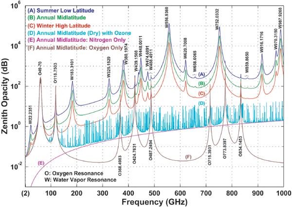
FIGURE 3.1 Atmospheric zenith opacity in the radio spectrum commonly used for the EESS. SOURCE: A.J. Gasiewski and M. Klein, The sensitivity of millimeter and sub-millimeter frequencies to atmospheric temperature and water vapor variations, Journal of Geophysical Research-Atmospheres 13:178481-17511, 2000, copyright 2001 by the American Geophysical Union.
utilize many of the same bands used by satellites to provide additional complementary measurements of the atmosphere.
Observations of Earth’s atmosphere, land areas, and oceans in the radio part of the electromagnetic spectrum have become increasingly important in understanding Earth as a system. Currently operational satellite sensors provide key meteorological data sets, including the Advanced Microwave Sounding Unit (AMSU) and instruments on the Defense Meteorological Satellite Program’s (DMSP’s) passive microwave weather satellites (the Special Sensor Microwave/Imager [SSM/I] and Special Sensor Microwave/Temperature [SSM/T]). Remote sensing satellite missions such as NASA’s Earth Observing System (EOS), European Space Agency’s (ESA’s) Soil Moisture and Ocean Salinity (SMOS), NASA/Japan Aerospace Exploration Agency’s (JAXA’s) Global Precipitation Measurement (GPM), and NASA’s Soil Moisture Active/Passive (SMAP) are providing information about water, rainfall, and ocean salinity on a global basis to improve measurements of atmospheric temperature, water vapor and precipitation, soil moisture, concentrations of ozone and other trace gases, and sea surface temperature and salinity. These multiyear, multibillion-dollar missions are international in scope, reflecting the interests of many countries in continued availability of accurate meteorological, hydrological, and oceanographic data and
measurements of land-surface features and trace gases in the atmosphere. It is critical to ensure continued data availability for these important applications. For example, the Tropical Rainfall Measurement Mission (TRMM) reached the end of its life in 2015 after providing unprecedented rainfall data for nearly two decades, much longer than its expected mission life of 3 years. In early 2014, the GPM was launched to provide continued and improved rainfall mapping and forecasting.
Techniques
Passive sensors have receivers that measure the electromagnetic energy emitted and scattered by Earth’s surface and the constituents of Earth’s atmosphere. Measurements at “opaque” frequencies are affected by the absorption and emission of the waves and are strong functions of frequency due to resonant absorption by atmospheric gases. Atmospheric gases emit and absorb microwave energy at discrete resonant frequency bands described by the laws of quantum mechanics, necessitating atmospheric observations in those bands (Figure 3.1). For example, atmospheric molecules of H2O have resonances at 22.235 and 183.3101 GHz, and frequencies near these resonances are needed for the measurement of water vapor by passive spaceborne sensors. Other atmospheric constituents with resonant frequency bands in the microwave spectrum include O2, O3, CO, NOx, and ClO. Measurements taken near the resonances of these gases can be used to determine the amount of the particular gas in the atmosphere. Oxygen lines around 55 GHz are used to obtain atmospheric temperature profiles, and water lines are used to obtain atmospheric humidity profiles. The frequency allocations needed for these measurements are rigidly determined by the location of the resonant frequency bands.
The choice of frequencies for measurements of Earth’s surface by passive sensors is not as tightly constrained as that for atmospheric measurements. If Earth were an ideal blackbody, then it would emit radio emission of intensity proportional to its temperature, and that is all that could be determined. However, the actual emission depends on the surface characteristics of land and water, such as roughness, soil moisture, and wind speed (see Figures 3.2 and 3.3). The sensing of many surface phenomena requires simultaneous measurements at several frequencies because the energy emitted at any given frequency is determined by several overlapping geophysical phenomena. Multiple frequencies either help separate the property of interest or provide a correction for competing factors such as variations in the sea surface temperature to estimate wind speed or absorption in the atmosphere. Within a set of approximately octave-spaced bands (Appendix B), suitable for particular applications, the precise frequencies to be used for sensing Earth’s surface are not critical. The selection of specific frequency is typically based upon the feasibility of sharing frequencies with other allocated radio services. Because passive radio astronomy services (Chapter 2) use these same windows to observe the universe from the ground, there is much spectrum compatibility between the two sciences. However, below 20 GHz, constraints on the parameters of active radio services may be needed to make spectrum sharing feasible.
The energy emitted from Earth’s surface is a function of frequency, surface roughness and dielectric properties, polarization, angle of incidence and aspect, and subsurface microstructure. A few underlying physical principles characterize the capabilities of most passive microwave techniques used in the “window” channels to observe Earth’s surface. First, lower-frequency waves generally penetrate intervening media better and sense deeper beneath the surface. Thus low frequencies such as those at L-band (e.g., 1.4 GHz, Appendix B) are preferred when sensing subsurface soil moisture beneath vegetative canopies. Second, the influence of surface roughness tends to be largest when the length scales of the roughness are comparable to the electromagnetic wavelength. This fact motivates the use of X-band (e.g., 10.7 GHz)
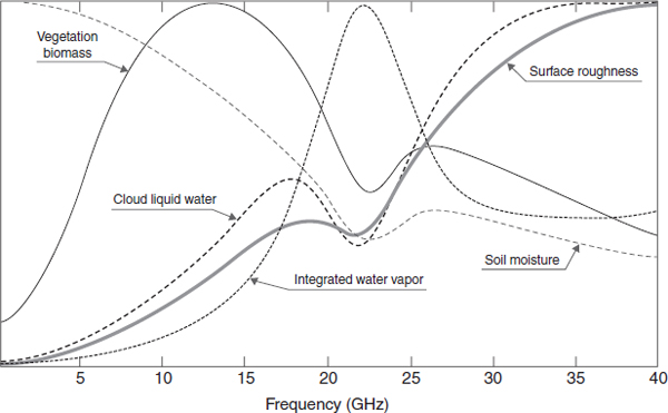
FIGURE 3.2 Relative sensitivity of brightness temperature to geophysical parameters over land surfaces as a function of frequency.
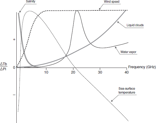
FIGURE 3.3 Relative sensitivity of brightness temperature to geophysical parameters over ocean as a function of frequency. SOURCE: Original figure by Thomas T. Wilheit, NASA Goddard Space Flight Center.
or higher frequencies in attempting to sense the short sea waves, such as the capillary waves, that are the most sensitive to sea surface winds at low wind speeds. Third, water in its various phases of ice, liquid, and vapor exhibits particularly strong characteristic absorption, emission, and scattering features in the radio spectrum. The dielectric constant of water is a strong function of frequency, temperature, and the water’s phase. Frequencies below approximately 2 GHz are the most sensitive to sea surface salinity, while the frequencies closer to 5-10 GHz are the most sensitive to sea surface temperature.
Sensors
A major tool of Earth remote sensing systems is the microwave radiometer. These passive sensors are similar in their basic design to radio astronomy receivers. The instrument sensitivity needed varies with the accuracy required for the physical property. For example, determination of open-ocean salinity, with typical values between 30 to 36 parts per thousand, requires accuracies on the order of 0.2 parts per thousand for use in numerical ocean models. In the 1-2 GHz range, where salinity is measured, this translates to a measurement sensitivity of about 0.1 K. Determination of soil moisture, which is also measured in this frequency range, requires accuracies of about 4 percent water by volume, with data availability every 2 to 3 days for meaningful use in weather prediction models. The sensitivity in this frequency band is about 1 to 3 K per percent soil moisture (hence a measurement requirement of about 4 to 12 K).
Scientists have conducted extensive studies to identify the frequencies needed for passive sensor measurements and to quantify the performance criteria of the sensors used by EESS, and to inform and complement the regulations formulated by the International Telecommunications Union’s Radiocommunication Section (ITU-R). The resulting frequencies are documented in Recommendation ITU-R RS.515 and the necessary bandwidths and sensitivities for various measurements are found in Recommendation ITU-R RS.1028. The ITU-R recommends that in shared frequency bands (except absorption bands), the availability of passive sensor data shall exceed 95 percent from all locations in the sensor service area in the case where the loss occurs randomly, and that it shall exceed 99 percent from all locations in the case where the loss occurs systematically at the same locations. For three-dimensional measurements of atmospheric temperature or gas concentration, the availability of data shall exceed 99.99 percent. Interference criteria have also been defined by the ITU-R. Permissible interference levels in dBW and interference reference bandwidths are contained in Recommendation ITU-R RS.1029. In bands that are allocated to EESS on an exclusive basis, it has been determined by the ITU that “all emissions shall be prohibited” (see Radio Regulation 5.340).
Techniques
Active microwave sensing involves radars. Radars receive signals that they have transmitted after these signals have been reflected by land or ocean surfaces or by water or ice particles in Earth’s atmosphere. Because the reflected signal depends on the dielectric properties of the surface and its roughness, the necessary frequencies for active sensing are determined by the phenomena to be measured. Generally speaking, bands spaced about an octave apart are needed (Appendix B), similar to those for the surface measurements using passive techniques and for the radio astronomy continuum measurements. The precise frequency used within the required octave-wide band is not critical, and the allocations are based upon other services within that band. The sharing of these bands, while not incurring or causing
interference with other sources, is an important modern-day consideration. For instance, sharing between active spaceborne sensors and terrestrial radars (the radiolocation service, in ITU parlance) has been shown to be feasible with certain design constraints, and the bands allocated for active sensing are all also allocated to the radiolocation service. The frequency bands to accommodate active sensor measurements range from below 1 GHz for surface measurements up to 150 GHz for cloud measurements. Applications of active sensors include the measurement of soil moisture and roughness, snow, ice, rain, clouds, atmospheric pressure, and ocean wave parameters, and the mapping of geologic and geodetic features and vegetation. Similar to passive requirements, the active sensor frequency and bandwidth requirements have been studied extensively by scientists, the results from which have informed the regulations at the ITU-R. These requirements can be found in Recommendation ITU-R RS.577.
Sensors
Major types of active sensors include spaceborne scatterometers and image-forming radars such as synthetic aperture radars (SARs) and Interferometric SAR (InSAR). SARs and InSARs are capable of determining topography and surface change over large geographic regions to unprecedented accuracy. Bandwidth requirements for active sensors vary with the type of application. For example, scatterometers are typically narrowband, low-resolution devices requiring about 1 MHz of bandwidth. Most SARs, precipitation radars, and cloud-profiling radars are medium-bandwidth devices; they can be designed to satisfy measurement resolution requirements in less than 100 MHz of bandwidth. However, altimeters and a few very-high resolution SARs require wide bandwidth, typically up to 600 MHz or more, to achieve desired measurement accuracies. Ultra-wide band radars for snow-depth profiling are now in experimental development and require several GHz of bandwidth but operate over a limited spatial extent.
Multispectral images obtained by SARs operating at 432-438 MHz, 1215-1300 MHz, 3100-3300 MHz, 5250-5570 MHz, and 9500-9800 MHz are used to study Earth’s ecosystems, climate, and geological processes, the hydrologic cycle, and ocean circulation. Altimeter measurements in the 5250-5350 MHz, 13.4-14 GHz, and 35-36 GHz bands provide data to study ocean-surface height and wave dynamics and their effects on climatology and meteorology. Spaceborne scatterometer measurements of ocean-surface wind speeds and direction in the 5250-5350 MHz, 9500-9800 MHz, and 13.25-14 GHz bands play a key role in understanding and predicting complex global weather patterns and climate systems. The GPM uses precipitation radars in the 13.4-14 GHz and 35-36 GHz bands to provide data on global rainfall. The Cloudsat mission, launched in May 2006, measures clouds using the recently allocated band at 94-94.1 GHz.
Performance and interference criteria for active spaceborne sensors have been extensively studied. These criteria have been defined in terms of the precision of measurement of physical parameters and the availability of measurements free from harmful interference. Interference criteria are stated in terms of the interfering signal power not to be exceeded in a reference bandwidth for more than a given percentage of time. The processing of SAR signals discriminates against interference depending on the modulation characteristics of the interfering signal and can materially improve the potential for sharing frequency bands. Performance and interference criteria for these sensors can be found in Recommendation ITU-R RS.1166.
In the following sections, the radio frequencies used by EESS for applications in atmosphere, terrestrial hydrology, cryosphere, oceans, and solid Earth and biosphere are discussed in more detail.
Systems for sensing atmospheric properties can be designed to exploit atmospheric absorption and emission resonances. There are a vast and growing number of applications that benefit from atmospheric measurements obtained by microwave and millimeter wave sounding instruments spanning research areas that include meteorology, oceanography, geology, and ecology. Measurements of the atmosphere using microwave radiometry have provided a benchmark climate record of temperature trends dating back to the first operational use of the Microwave Sounding Unit (MSU) in 1979, which began operation in 1979. MSU was followed by the Advance Microwave Sounding Unit, which began operation in 1998. The Advanced Technology Microwave Sounder (ATMS) is the first in a series of new cross-track scanning sounders developed for the Joint Polar Satellite System (JPSS). ATMS was launched on October 28, 2011, on the Suomi National Polar Partnership satellite. The Special Sensor Microwave Imager/Sounder (SSMIS), launched in 2003 on a DMSP satellite, observed atmospheric temperature up into the mesosphere as well as surface phenomena such as near-surface wind speed and sea surface temperature. The first Microwave Limb Sounder (MLS) was aboard the Upper Atmosphere Research Satellite (UARS), which was launched in 1991. The MLS provides measurements of stratospheric ClO, O3, and H2O, upper tropospheric H2O vapor and cloud ice, stratospheric HNO, and temperature variances associated with atmospheric gravity waves, as shown in Figure 3.4.

FIGURE 3.4 Daily observations of temperature, CO, H2O, O3, HCl, and OH from the Microwave Limb Sounder on the Earth Observing System-Aura satellite January 3, 2015. NOTE: Produced on February 25, 2015 12:47:48 using plot version 1.34. Courtesy of NASA/JPL; produced by the MLS Science Team at the Jet Propulsion Laboratory, California Institute of Technology, under contract with NASA, from EOS MLS and GMAO data: JPL Clearance CL#05-3463.
Observations of molecular absorption lines between 118 GHz and 2.5 THz, through the limb of the atmosphere provide key information on atmospheric chemistry from the upper troposphere through the stratosphere. Observations of O3 play an important role in monitoring the recovery of the ozone hole
In this section, we review the frequencies used for the atmospheric applications in the following areas: temperature and water vapor profiling, precipitation, atmospheric chemistry, clouds, and ionospheric sensing.
Atmospheric profiles of temperature, that is, temperature as a function of altitude, from polar-orbiting satellites are required to initialize and to update the current and emerging global ocean-atmosphere models that provide essential global meteorological and oceanographic predictions for many civil and military applications. High measurement accuracies are essential for the proper operation of these prediction models. For example, it has been shown that for temperature profile inputs not meeting the uncertainty criterion of 1 to 3 K (depending on altitude), the profile data corrupt the model rather than increase its capability to forecast. Observational errors, usually on smaller scales, amplify the model error and, through nonlinear interactions, gradually spread to longer scales and seriously degrade the forecast.
Currently, the temperature profiles are measured using low Earth orbit (LEO) satellite microwave sounders operating in the O2 absorption band from 50-62 GHz. A number of present-day technological developments are enabling the future deployment of geostationary orbiting microwave temperature sounders. The atmospheric attenuation on a clear day typically varies from ~1 dB near 50 GHz to >200 dB in the region 58 to 62 GHz. Atmospheric temperature profiles can be measured with an uncertainty of 1 to 3 K with vertical resolution ranging from 2 to 5 km (depending on altitude). The Defense Meteorological Satellite Program (DMSP) Special Sensor Microwave Imager Sounder (SSMIS) uses frequencies between 60.4 and 61.2 GHz and a separate channel near 63 GHz to obtain mesospheric temperature profiles. The same oxygen resonance frequency that enables these measurements also leads to the strong absorption of terrestrial anthropogenic emissions. In many (albeit not all) cases, the spectrum from approximately 58 to 62 GHz can be shared with terrestrial ground-based active systems, such as point-to-point communication systems.
The atmospheric temperature profiles can also be derived using passive radiometric measurements on and near the 118.75 GHz O2 transition. Temperature profiles derived from this band complement those derived using the 50-60 GHz band by providing independent measurements, albeit with reduced sensitivity at higher altitudes and less penetration of clouds and precipitation. However, diffraction-limited apertures of fixed size will yield temperature profiles with better horizontal spatial resolution with 118 GHz measurements compared with the data from 50-60 GHz. As a result, channels near 118 GHz are being considered for use in sounding and imaging from geostationary microwave sensors. Moreover, the difference in response between similar clear-air channels at 50-60 GHz and ~118 GHz will provide additional information on cloud and precipitation amounts.
The hydrologic cycle is critical to the dynamical and thermodynamical functioning of the global climate system and to its impacts on human society. The distributions of water vapor, cloud liquid water, and cloud ice in the atmosphere and the evolution of these distributions with time determine to a great extent the radiation characteristics of clouds, with consequent large impacts on the radiation balance of the atmosphere. Much of the atmospheric moisture is concentrated close to Earth’s surface in the lowest ~1.5 to 2.5 km
of the atmosphere. Water vapor is an important greenhouse gas, greatly influencing the surface radiation budget even in the absence of clouds. Condensation and evaporation of water in the atmosphere affect large transfers of energy and have enormous influence on large-scale circulation in the troposphere. The global water vapor measurements are essential to initialize and to update meteorological forecasting and climatological models that provide the global meteorological and oceanographic predictions necessary for civil and military operations. Comparisons of model simulations indicate that if the measurement accuracies of moisture profiles are less than threshold values (typically set to 20 to 35 percent of the root mean square mass mixing ratio), then the remotely sensed profile data that are used as input corrupt the model. Combined microwave and infrared spectral data can yield what is nearly all-weather global performance, even in most cloudy conditions. Moisture profiles can also be used to support path delay and attenuation estimates for active remote sensing systems (e.g., radar altimeters) and satellite radio-frequency links. Accurate measurements of upper tropospheric water vapor are also obtained by viewing Earth’s limb from LEO to support scientific studies of the upper atmosphere and associated atmospheric chemistry.
Radar observations are strongly dependent on unknown drop size distributions, and optical sensors do not penetrate clouds well; thus microwave radiometers on all types of platforms (satellite, aircraft, ships, and ground sites) are essential to making water vapor measurements. Passive measurements near the strong 183.31 GHz water-vapor line, aided by measurements in the adjacent transmission window at the EESS-allocated bands of 150-151 GHz or 164-168 GHz, are critical for the global measurement of atmospheric water vapor profiles. Measurements from spaceborne sensors in LEO are carried out to obtain atmospheric water-vapor profiles from Earth’s surface to 100 mb with a measurement uncertainty of approximately 20 to 35 mb. Two different types of microwave observations are used: those in transparent bands within which the warmer water vapor absorption stands out (1) against the colder ocean background (ocean partially reflects the extremely cold cosmic background radiation (see Section 2.5.1) or (2) against that of cold low-emissivity land.1 No profile information is usually retrieved—only an estimate of the column integrated abundance. The frequencies most often used for this purpose include 18.7, 22, 23.8, 31.4, 37, and 89 GHz. To improve retrieval accuracies, these channels are often dual-polarized (horizontal and vertical) and scanned at a near-constant angle of incidence (e.g., GPM Microwave Imager [GMI], Special Sensor Microwave/Imager [SSM/I], Special Sensor Microwave/Imager Sounder [SSMIS], WindSat, and Advanced Microwave Scanning Radiometer [ASMR]-E). In addition, the opaque water vapor resonance near 183 GHz is often used by measurements in the adjacent transmission window at the EESS-allocated bands of 150-151 GHz or 164-168 GHz; these can also be used in combination with temperature profile information to yield the most accurate results (e.g., AMSU, SSMIS). Figure 3.5 shows the water vapor derived from the SSM/I. Instruments retrieving water vapor profiles are generally used to retrieve other parameters simultaneously, such as cloud water content, precipitation rate, and ice and snow cover information.
3.2.3 Integrated Precipitable Water
Integrated precipitable water or total precipitable water (TPW), that is, the total atmospheric water vapor from the surface to 30 mb, can be estimated to an uncertainty of <2 mm or ~10 percent (millimeters of condensed water) using space-based radiometric measurements in the K-band (Appendix B). These measurements are of major use for meteorological research and forecasting and for astronomical and military applications. Radiowave propagation delays due to atmospheric water vapor can also be derived from radiometric measurements in the spectral region near 22 GHz.
_____________
1 For background regarding EESS for water vapor profiling, see the following: J.R. Wang, P. Racette, and L.A Chang, MIR measurements of atmospheric water vapor profiles, IEEE Transactions of Geoscience Remote Sensing 35(2):212-223, 1997.
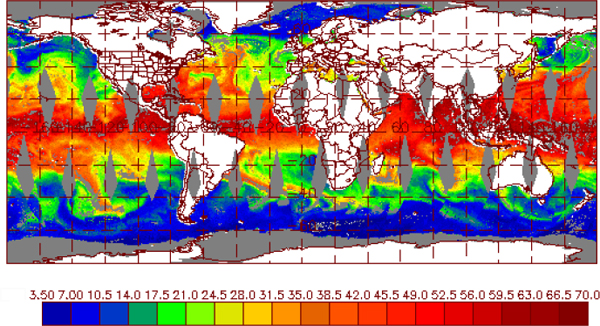
FIGURE 3.5 Operational water vapor (in kg/m2) product over ocean for June 13, 2015. The data derived from the SSM/I sensor on the DMSP satellites relies on measurements at 19.35, 22.235, and 37 GHz. SOURCE: Courtesy of NOAA Office of Satellite and Product Operations, National Environmental Satellite, Data, and Information Service; see “SSM/IS Products” at http://www.ospo.noaa.gov/Products/land/spp/ssmis.html.
For an estimate of the total columnar water, the optimum frequency is one for which the water-vapor-density weighting function has a constant profile with height. Weighting functions in the region of the 22.235 GHz weak water vapor absorption line display these characteristics and are widely used as the primary radiometric channel for estimates of TPW (see Figure 3.6) and path delay. It is noted that the same bands that are used to measure water vapor from space are also used on ground- and ship-based radiometers to measure TPW from the surface of Earth. These ground-based sensors are becoming widely used around the globe to help initialize and update numerical weather-prediction models and for the calibration of remote sensing satellites. Although they do not provide global measurements, they are particularly accurate over both land and water, because they view water vapor against a strong contrasting background caused by the cold cosmic emission temperature of 2.73 K (see Section 2.5.1).
Accurate measurement of spatial and temporal variations of rainfall around the globe, particularly over the vast and under-sampled Southern Hemisphere, and oceanic and tropical areas, is one of the most difficult and important problems in meteorology. Satellite-based microwave remote sensing of precipitation can provide the best-available means of obtaining data detailing four-dimensional distribution of rainfall and latent heating on a global basis.2 Rainfall and snowfall rates and total amounts of
_____________
2 For background information regarding EESS for precipitation and clouds, see the following: G.L. Stephens and C.D. Kummerow, The remote sensing of clouds and precipitation from space: A review, Journal of Atmospheric Science 64:3742-3765, 2007.

FIGURE 3.6 Total precipitable global water product. Data from multiple satellites are merged to produce global nearly continuous products which track the flow of water vapor and are key to weather forecasting. SOURCE: Courtesy of NOAA Office of Satellite and Product Operations, National Environmental Satellite, Data, and Information Service; see “The NESDIS Operational Blended TPW Products” at http://www.ospo.noaa.gov/Products/bTPW/TPW_Animation.html?product=GLOBAL_TPW.
precipitation are highly valuable measurements that can be determined by on-orbit and ground-based microwave and millimeter wave radiometers. Knowledge of these quantities is important to the prediction of floods, crop health and yield, and catchment replenishment for hydroelectric, irrigation, and domestic uses, and for other societal benefits and impacts. The link between precipitation and clouds provides important constraints on climate variability through the Earth radiation budget. Precipitation measurements using microwave remote sensing may utilize both active and passive sensing. Rain mapping using radar reveals the three-dimensional structure of precipitation, such as the observations from the GPM as shown in Figures 3.7 and 3.8. These radar observations can be used to develop statistical cloud and rain-cell models and to provide improved calibration of rainfall measurements derived using passive radiometry alone. In general, microwave radiometric measurements within the bands at 6, 10, 18, 23, 37, and 89 GHz are of primary interest for rainfall measurement. Active measurements of precipitation are carried out near 13.6, 35.5, and 94 GHz.
Passive microwave measurements near the 89 GHz atmospheric window play an important role in the retrieval of precipitation data, particularly over land. Owing to the combination of high emissivity, thickness, and temperature of clouds over land, signatures of convective precipitation cells are often strongest at 89 GHz. At this frequency there is high sensitivity to clouds over land, causing the upwelling brightness temperatures to be cooler rather than warmer, as observed over a relatively cold ocean background. Clouds over land exhibit much less contrast at lower microwave window frequencies (e.g., 10, 18, and 37 GHz) causing 89 GHz observations to play an important role in determining rain rate over land.
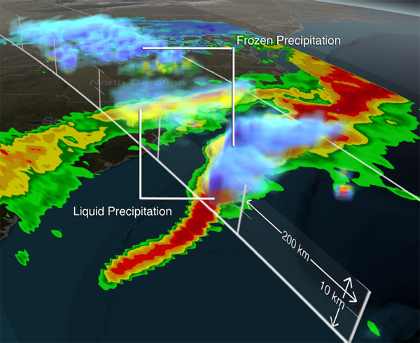
FIGURE 3.7 A storm in the eastern United States observed by the NASA/JAXA Global Precipitation Measurement (GPM) Core Observatory on March 17, 2014. A full range of precipitation, from rain to snow was revealed by the GPM measurements. SOURCE: Courtesy of NASA/JAXA; see NASA GSFC, “GPM Data from March 2014 East Coast Snowstorm,” image, March 17, 2014, http://pmm.nasa.gov/image-gallery/gpm-data-march-2014-eastcoast-snowstorm.
Passive microwave remote sensing from satellites and aircraft at frequencies above 90 GHz are used to estimate hydrometeor properties of cirrus clouds and the higher altitude convective and anvil clouds, which contain frozen particles. Specific frequencies currently used include 150 GHz, 166 GHz, 183.31 GHz, 220 GHz, 325 GHz, 340 GHz, 380 GHz, 424 GHz, ~500 GHz, and 640 GHz. These channels are particularly sensitive to the frozen particles, and several have been used to estimate snowfall rates over land surfaces. Furthermore, because these channels tend to become opaque to the land surface in the presence of clouds, they may be useful in estimating light rain over land surfaces. Precipitation observations may also be possible with high spatial resolution using a geostationary microwave sounder at frequencies of ~50, 89, 118, 183, 340, 380, and 424 GHz.
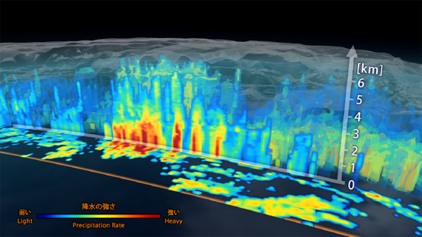
FIGURE 3.8 The Global Precipitation Measurement mission’s dual-frequency precipitation radar observed a three dimensional structure of precipitation, inside an extra-tropical cyclone off the coast of Japan on March 10, 2014. The image shows rain rates across a vertical cross-section approximately 4.4 miles (7 kilometers) high. The red areas indicate heavy rainfall while yellow and blue indicate less intense rainfall. SOURCE: Courtesy of JAXA/NASA; see NASA, “First Images Available from NASA-JAXA Global Rain and Snowfall Satellite,” Release 14-086, March 25, 2014, http://www.nasa.gov/press/2014/march/first-images-available-from-nasa-jaxa-globalrain-and-snowfall-satellite/#.VhakDflVhBe.
Among the most important of human influences on climate is the production of greenhouse gases, including CO2, methane (CH4), and various chlorofluorocarbon (CFC; hydrochlorofluorocarbon [HCFC]) and hydrofluorocarbon (HFC) compounds. Of these, CO2 and CH4 rapidly become well mixed in the lower atmosphere and affect Earth’s radiation budget by trapping infrared radiation that would otherwise be expelled to space. Although CO2 and CH4 are themselves potent greenhouse gases and the primary cause of observed global warming, their indirect influence on atmospheric water vapor—a more potent and less predictable greenhouse gas—is perhaps even more important. Tropospheric water vapor provides a feedback mechanism through which increased global warming adds to the capacity of the atmosphere to contain water vapor while simultaneously elevating evaporation rates. The monitoring of water vapor and cloud water content and their effects on global radiation fluxes is thus critical to understanding the causes of climate change and predicting future climates. Currently, cloud coverage and type are the most significant sources of uncertainty in global climate modeling. Climate is also strongly affected by trace gases in the upper troposphere, stratosphere, and mesosphere; some of these trace gases also facilitate the destruction of stratospheric ozone. A diminished ozone layer allows harmful ultraviolet-B (UV-B) radiation from the Sun to reach Earth’s surface, where it significantly enhances the probability of the
occurrence of basal and squamous cell skin cancers and cataracts. The underlying chemical reactions that cause ozone depletion require chlorine and bromine to be present in sufficient quantities in the stratosphere.
Passive microwave observations provide a uniquely valuable means for monitoring the distribution and concentration of ozone and other trace gases including source, reservoir and active forms of key ozone-depleting substances, other species involved in ozone layer chemistry, and long-lived tracers used to track motions of air parcels. The first Microwave Limb Sounder (MLS) on NASA’s Upper Atmosphere Research Satellite used channels near 63, 183, and 205 GHz to measure emissions of chlorine monoxide (ClO), water vapor, ozone (O3), and sulfur dioxide (SO2). ClO is a key reactant in the chlorine chemical cycle that destroys O3. A second generation MLS instrument is on NASA’s AURA spacecraft (launched in July 2004); it uses channels near 118 GHz for temperature and pressure profiling, 190 and 183 GHz for HNO3 and water-vapor measurements, 240 GHz for O3, and 640 GHz and 2.5 THz to support detailed studies of the stratosphere and the chemistry associated with ozone depletion. Instruments making passive observations Earth’s atmospheric composition under development use frequencies listed above, plus the 320-360 GHz spectral region. Mesospheric O3 can be measured using an 11.072 GHz line using radiometer techniques and measurements from 50 to 80 km and 80 to 104 km can be made using ground-based receivers.
As described earlier, clouds play an important role in both Earth’s water and radiation budgets. Determination of the composition, structure, and location of clouds is of critical importance for numerical weather and climate modeling and analysis. Microwave radiometric measurements within the bands at 6, 10, 18, 23, 31, 37, and 89 GHz are of primary interest for clouds. Active measurements of clouds are carried out near 13.6, 35.5, 78.5, and 94 GHz. It is important to have knowledge of cirrus clouds and the frozen particles in convective and anvil clouds for several reasons: (1) to enhance cloud-resolving models, (2) to better understand the relationships between the frozen and melting particles, (3) to clarify relationships between the passive observations and frozen particles, (4) to improve latent heating and global change models that are particularly sensitive to cirrus ice clouds and to the ice in convective and anvil clouds, and (5) to provide indirect information on surface rain rate below the cirrus anvil. Finally, real-time estimates of snowfall rate are extremely useful for urban management.
Cloud ice water path (CIWP) is the vertically summed mass of cloud-borne ice particles per unit of area. As ice clouds can reflect a significant amount of sunlight, their impact on global radiative energy fluxes, and hence climate change is considerable. Future global CIWP measurements from space, using passive microwave techniques at frequencies from 89 GHz up to approximately 1 THz (e.g., 150, 166, 183, ~220, and ~340 GHz) could characterize the coupling of the global hydrologic and energy cycles through upper tropospheric cloud processes. Retrieval of CIWP data depends strongly on knowledge of the cloud particle size distributions. Therefore, retrievals are improved using multiple high-frequency brightness temperature measurements. Such measurements would enable the development and testing of new self-consistent parameterizations of ice cloud processes and cloud systems, which could in turn guide improvements in ice cloud representation in global Earth system models. These improvements will significantly advance the understanding of the hydrological cycle and climate predictability. The inclusion of cloud microphysics into cloud and climate models within the decade is anticipated by many numerical weather modelers. Accordingly, measurements of cloud ice water will be needed to diagnose and validate these cloud models, which, in principle, have the ability to greatly improve the understanding of climate, rainfall, and precipitation variability and the atmospheric radiation budget.
A spaceborne 94 GHz cloud-profiling radar (CloudSat) was successfully launched in May 2006, with an objective of measuring the altitude and properties of clouds with 500 m vertical resolution, 1.2 km cross-track resolution, and with a sensitivity of –30 to –36 dBZ (decibels of Z, where Z is the energy reflected back to the radar, or reflectivity). This advanced W-band radar (Appendix B) has provided information on the vertical structure of highly dynamic cloud systems to provide global measurements of cloud properties, as shown in Figure 3.9. These measurements have helped scientists compile a database of cloud properties to improve the representation of clouds in global climate and numerical weather-prediction models.
Cloud base information for a range of cloud types, particle distributions (microphysics), and liquid water content is desired to support both operational and scientific objectives. Ceiling height data are vital to identify regions of potential aircraft icing and for determining the most effective altitudes for commercial flight operations. For climate measurements, cloud base height is critical for determining the long-wave energy budget at Earth’s surface, and for understanding the impacts of anthropogenic aerosols on cloud formation, precipitation, and short- and long-wave energy fluxes.
For non-precipitating clouds, microwave radiometric brightness temperatures near 10, 18, and 37 GHz can be used to estimate the integrated amount of cloud liquid water to within approximately 0.05 mm or 10 percent total columnar water precision. Within the next 5 to 10 years, inclusion of cloud microphysics in climate models is expected. Measurements of cloud liquid water will be needed to diagnose and validate these cloud models, which in principle have the ability to greatly improve understanding of climate, rainfall variability, and the atmospheric radiation budget. The inclusion of cloud water into numerical weather-prediction models will also provide an important means of accurately
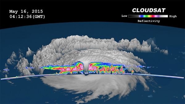
FIGURE 3.9 Combined imagery from Cloudsat and Japanese Multifunctional Transport Satellite (MTSAT) of Typhoon Dolphin in the West Pacific on May 16, 2015. SOURCE: Courtesy of NASA/JPL-Caltech/Colorado State University; see NASA, “Dolphin (was 07W/System 93W - NW Pacific Ocean),” May 21, 2015, http://www.nasa.gov/feature/dolphin-was-07wsystem-93w-nw-pacific-ocean.
modeling the influences of short-wave and long-wave radiation on the evolution of severe weather. Accurate measurements of cloud water amounts also play an important role in global climate models and in understanding the impact of anthropogenic and natural aerosols on clouds, rainfall, and climate. As with water vapor, the same bands that are used to measure cloud liquid water from space are also used on ground- and ship-based radiometers to measure cloud liquid water from Earth’s surface, but with greater accuracy because of the cold cosmic (see Section 2.5.1) background. Widespread global deployment of these sensors is occurring.
Radio frequencies are used to understand the physical state of the ionosphere, characterize irregularities, detect large-scale structures, and enable the real-time monitoring and prediction of propagation conditions and space weather effects. Such understanding enables important scientific and commercial applications including communications, precision navigation, environmental remote sensing, and national defense. Techniques for remote sensing of the ionosphere include study of ionospheric coupling to the lower atmosphere below and the larger heliospheric environment above, using both passive and active techniques over a wide range of frequency bands. In this section, we briefly survey ongoing work and point out the wide range of frequencies below 3 GHz that are used for ionospheric sensing.
Passive microwave techniques involve monitoring of the radio spectrum, radio imaging and interferometry, precision measurement of radio noise, and passive use of transmitters of opportunity (natural or man made) to measure ionospheric phenomena. Riometers (relative ionospheric opacity meters) such as IRIS, KAIRA, and EDGES, measure ionospheric absorption and provide images of ionospheric structures in the frequency range of 20-70 MHz. Frequencies lower than 20 MHz tend to be contaminated by broadcast signals, while those higher than 70 MHz have high absorptions in the D- and F-regions of the ionosphere.
Radio scintillation is used for real-time amplitude and phase fluctuations detection of ionospheric conditions such as plasma parameter gradients and embedded irregularities. These impact trans-ionospheric propagation and detection of heliospheric phenomena. Interplanetary scintillation is used for detection of electron densities and magnetic field of coronal mass ejections at distances <1AU. It is measured at a variety of frequencies from HF to S-band (Appendix B). Satellite and ground-based phase coherent radio beacons measure total electron content (TEC) and the amplitude and phase fluctuations in the trans-ionospheric signals (i.e., scintillations) related to the irregularities along the propagation path. Example frequencies of the currently on-orbit beacons operate at 150.012, 300-400, 400.032, 1066.752, and 2360-2380 MHz; and on-ground beacons operate at 401.25 MHz and 2036.25 MHz. Examples of space-based receiver frequencies include 150, 400, and1067 MHz. Both active transmissions from satellites and observation of radio star scintillation (RSS) are routinely conducted. Global Navigation Satellite System use navigation signals in L1 (1575.42 MHz), L2 (1227.6 MHz), and L5 (1176.45 MHz) bands to estimate ionospheric delay.
In the low frequency ranges, VLF sounding techniques are used for magnetosphere-ionosphere coupling, field-aligned TEC, wave perturbations, wave-particle interactions, and lightning locations. ELF from 1-800 Hz are used to explore Schumann resonances in the Earth-ionosphere waveguide cavity and are important for Q-bursts due to “super-bolt” lightning strikes and “sprites” associated with these large strikes. The ULF from 10-4 to 1 MHz are used for magnetosphere-ionosphere coupling, provide remote sensing of natural wave modes, and magnetospheric resonances. Low frequency radio telescopes (e.g., LOFAR, MWA, VLA, or LWA) produce calibration products that provide very accurate all-sky map of relative line integrated electron density between baselines. Existing systems with frequency ranges of 10-300 MHz and future systems such as SKA and RAPID can be used to study small-scale ionospheric waves and structures. Satellite-based HF receivers are used to study manmade and natural
HF waves such as radar propagation, lightning pulses, HF scatter from ocean, and high-power HF interactions in the ionosphere at 0-18 MHz range (e.g., ePOP and CARINA).
Passive radar observations of the ionosphere uses transmitters of opportunity such as AM and FM radio, and HDTV, to produce radar observations. These observations are used to study propagation and scattering in the ionosphere, ionospheric turbulence, natural plasma irregularities, and meteor trails. White space bands between stations are often useful for passive propagation measurements in bi-static and multi-static receiver configurations. In-band on channel digital radio, such as used with FM, acts to jam these configurations.
Active techniques are also used for ionospheric sounding, noise and absorption measurements, and radio propagation-based techniques (both ground-to-ground and ground-to-space). Incoherent scatter radar provides precise measurement of the thermal ionospheric plasma. Primary measurements include electron density, electron temperature, ion temperature, and ionospheric drifts and provide information on electric fields, neutral winds, and ion compositions. Typical HF/VHF/UHF/L-band center frequencies, with up to 30 MHz bandwidth on receive and typically up to 1 MHz bandwidth on transmit, are used in existing systems. Up to 10 MHz bandwidth is planned for future systems. Significant power aperture is required, with most systems being multi-megawatt class that have antennae sizes between 25 and 300 meters. Current active systems operate at 46.5, 47, 49.92, 53.5, 154-162, 224, 430, 440, 440.2, 440.4, 442.5, 449.3, 500, 933, 1290, and 2380 MHz, with future systems planned at 220 and 233 MHz.
Ionospheric sounders or ionosondes provide direct measurement of ionospheric electron density profiles using transmissions that experience total reflection at the local plasma/Langmuir frequency. Because electron density and hence the resonance frequency is altitude dependent, these systems must span a significant range (e.g., ~ 1 to 15 MHz), which is time-dependent based upon geophysical conditions. Altitude coverage is limited by the peak ionospheric cut-off frequency. Higher frequencies beyond the local plasma frequency can be used for oblique sounding up to 30 MHz. The pseudorandom transmission radar sounders with low emission levels that produce minimum electromagnetic interference levels (~ 1 W) and low power noise-like radar transmissions can be used to produce HF range-Doppler radar measurements and even ionosonde measurements. This type of radar, which is currently being developed, would cause less interference to other users of the already crowded HF band. They operate from 2-30 MHz with typical bandwidths of 100 kHz. Transmission at low power covering the entire frequency range can be very useful for high measurement speeds. Similar to ionosondes, they provide measurements of electron density and reflection height, wave measurements, meteor trails, and Doppler radar measurement of coherent scattering structures.
The mesosphere/stratosphere/troposphere radar systems measure the lower boundary of the Geospace environment and its coupling to the ionosphere and lower atmosphere. They operate at 30-60 MHz, VHF/UHF, and S-bands. The Mesosphere/Lower Thermosphere (MLT) dynamics radars provide measurements of the mesosphere regions. The mesosphere is a crucial atmospheric layer and is quite difficult to observe by techniques other than meteor radar (MR) and medium frequency (MF) radar that operate at 2-3 MHz. These radar measurements have widely been used to detect mean winds and tides and to get insight into the seasonal, interannual, and long-term behavior of the MLT circulation including long-term trends. In addition, MR and MF radar measurements have been combined to analyze properties of planetary waves and estimate wind parameters. Meteor radars, operating at 30-50 MHz, with some systems operating from 2-100 MHz, provide neutral wind measurements by measuring the Doppler frequency of a drifting meteor trail after the meteor has ablated in the upper atmosphere.
Radars at 2-10 MHz (some specific examples, 2.8, 3.5, 3.85, 5.1, 8.175 MHz) are used to heat the ionosphere at an altitude where the critical frequency corresponds to the transmission frequency. The measurements can be used to investigate fundamental plasma physics primary and secondary wave
modes in the plasma, and to measure ionospheric parameters inaccessible by other means. High-power HF have produced artificial aurora, enhanced ionization, field-aligned irregularities, and stimulated electromagnetic emissions.
HF radar operating between 5-50 MHz is used for over the horizon observations of a variety of targets and for ionospheric measurements. Wide-Sweep Backscatter Ionograms are used by over-the-horizon radars to map the HF propagation conditions over ~1000 km in range. Measurement of coherent scattering structures at HF allows detailed study of ionospheric irregularities and plasma physics. Propagation and surface scattering effects, ionospheric waves from earthquakes, or just traveling ionospheric disturbance and Alfven waves can also be investigated.
Soil moisture (SM) is a key component of the land-surface hydrospheric state and is vital to weather and climate prediction research. It is essential in estimating latent heat and carbon fluxes at the land-atmosphere boundary. SM is also a key parameter in forecasting relating to agriculture, drought, and flooding and for predicting vegetative stress and establishing related government policies. Accurate knowledge of the parameters of SM has been shown to improve forecasts of local storms and seasonal climate anomalies. Atmospheric models tend to use sea surface temperatures (SSTs) as their primary boundary condition because so much of Earth’s surface is ocean. However, models just using SSTs are unable to capture seasonal climate anomalies in the middle of large continents. However, if SM data are incorporated, atmospheric models can accurately predict the seasonal anomalies in extreme weather.
Passive microwave radiometers operating at frequencies of 10 GHz and lower are sensitive to variations in soil density, type, and moisture content and are needed for SM measurements.3 Radiometry in the 1-2 GHz range is arguably the best means for measuring subsurface soil moisture on a national or global basis. A combination of active and/or passive microwave measurements can be used to remotely sense SM under moderately vegetated areas, with up to ~5 kg/m2 of vegetation water content. These measurements provide SM information with an uncertainty of 0.04 m3/m3. Passive measurements rely on the dependence of the microwave emissivity of soil to its water content. Lower microwave frequencies provide good soil penetration depth, permitting measurements of soil moisture down to ~10 cm depth at 1.4 GHz, and less so at higher frequencies. Active measurements, such as those at 1.26 GHz, rely on the dependence of soil backscatter on water content and are complicated by surface roughness and scattering by vegetation cover. Active measurements can, however, provide finer spatial resolution than is possible with passive techniques. Thus, a combination of active and passive measurements, such as those from the NASA SMAP mission, can be used to separate the effects of surface roughness and vegetation scattering from the soil-moisture signature while providing the desired spatial resolution, as shown in Figure 3.10. Passive microwave measurements in the C-band region, near 6.8 GHz, such as those from AMSR-E and AMSR2, can be used to infer soil moisture in the top 1cm of the surface layer under bare soil and lightly vegetated areas with water content up to ~2 kg/m2, to an approximate accuracy of 0.10 m3/m3.
_____________
3 For background information regarding EESS for soil moisture see the following: W. Wagner, P. Pampaloni, J.-C. Calvet, B. Bazzari, J.P. Wigneron, and Y. Kerr, Operational readiness of microwave remote sensing of soil moisture for hydrologic applications, Nordic Hydrology 38(1):1-20, 2007; J. Judge, Microwave remote sensing of soil water: Recent advances and issues, Transactions of the American Society of Agricultural Engineers–Centennial Edition 50(5):1645-1649, 2007.

FIGURE 3.10 Global soil moisture from L-band observations of the NASA SMAP mission at a spatial resolution of 10 km obtained by combining passive measurements at a spatial resolution of 36 km with active measurements at a spatial resolution of 3 km. SOURCE: Courtesy of NASA/JPL-Caltech/GSFC; see NASA/JPL, “SMAP’s Radiometer Captures Views of Global Soil Moisture” April 22, 2015, http://smap.jpl.nasa.gov/resources/87/.
The seasonal freeze-thaw transition of the Northern Hemisphere is a significant source and sink of atmospheric CO2. The exact timing of the spring thaw and the resulting length of the growing season can fundamentally affect the net carbon exchange budget between land and atmosphere. The thawing of polar tundra also results in more solar absorption and heating, with the possible runaway production of methane from the anaerobic decomposition of sub-surface biomass. Because microwave signatures are directly sensitive to the liquid and the solid phase of water, both active and passive observations are well suited for monitoring global freeze-thaw. The radar response to the freeze-thaw transition dominates the response due to any other factors such as changes in canopy structure, biomass, or precipitation. Typically, time series change detection approaches have been used to obtain freeze-thaw information from scatterometers operating at L-band (1.2 GHz; Figure 3.11), C-band (at 5.3 GHz), or Ku band (at 13.4 GHz). The passive approaches rely on the differing sensitivities among various frequencies to liquid moisture and volume scattering, thus requiring multi-frequency observations. Spectral gradients between various frequency combinations at 6, 10, 18, 22, and 37 GHz have been used to obtain freeze-thaw.
Fresh water is essential to all life forms. Our ability to measure, monitor, and predict the global supply of fresh water is increasingly valuable as many countries face critical challenges in meeting demands for clean water supplies partly because of growing and shifting populations. Knowledge of the location, extent, and changes of surface water bodies such as rivers, lakes, reservoirs, floodplains, and wetlands is
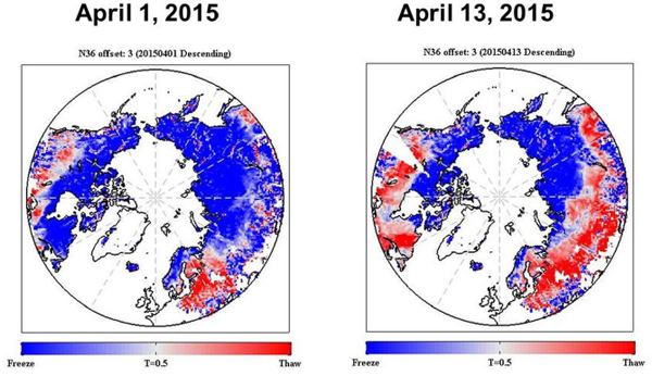
FIGURE 3.11 Spring thaw as observed by the radar at L-band aboard the NASA SMAP mission. SOURCE: Courtesy of NASA/JPL-Caltech; see “SMAP Shows Progression of Spring Thaw,” April 2015, http://smap.jpl.nasa.gov/resources/85/.
also important for predicting impacts of extreme hydrological events such as floods. In addition, inundated areas such as the wetlands contribute about 25 percent of the annual CH4 emissions to the atmosphere, affecting the carbon budget. To date, our ability to measure, monitor, and predict the spatial extent and variability of fresh water at the global scale is surprisingly poor. Specific measurements that are needed to obtain such knowledge are the elevation of the water surface, its slope, extent, and temporal change.
Satellite-based microwave sensors are well suited for measuring these parameters. For example, radars operating at L, C, Ku, and Ka bands have been used to measure surface water extent, elevation, and temporal variations using combinations of altimetry, imaging, and interferometric techniques. Sensors at L-and C-bands, in particular, can also provide information regarding seasonal inundation extents in floodplains and wetlands using both active and passive measurement techniques. At L- and C-band, passive signatures typically decrease with increasing inundation, while active signatures are typically low over flat, open water, but high where dense vegetation is inundated because tree trunks act as corner reflectors.
The cryosphere consists of components of the Earth system that contain water in a frozen state. Glaciers, ice sheets, snow cover, lake and river ice, and permafrost make up the terrestrial elements of the cryosphere. Sea ice, frozen sea-bed, and icebergs constitute the oceanic elements of the cryosphere. This definition of Earth’s cryosphere implies that substantial portions of Earth’s land and ocean surfaces are directly subject in some fashion to cryospheric processes. As such, observations of the cryosphere are necessary to predict future variability in Earth’s ice cover, and its interaction with other Earth systems must be made on commensurate spatial and temporal scales. Moreover many measurements must be made
TABLE 3.1 Radio-Frequency Sensors Supporting Cryosphere Research
| Platform/Sensor | Example Cryo Application | Center Frequency |
| Currently Operational Spaceborne | ||
|
SMAP/Radiometer |
Sea ice and ice sheet | 1.41 GHz |
|
GCOM/AMSR-2 |
Sea ice concentration, snow cover, wet/dry snow, dry snow water equivalent | 18.7, 36.5, 89.0 GHz (Cryo used) Possible 6.925 app |
|
DMSP/SSMI |
Sea ice concentration, snow cover, wet/dry snow, dry snow water equivalent | 19.35, 37, 85 GHz |
|
SMOS/MIRAS |
Sea ice thickness, ice sheet morphology, seasonal snow cover | 1.41 GHz |
|
Sentinal |
Sea ice monitoring, glacier/ice sheet motion | 5.405 GHz |
|
Radarsat 2 |
Lake/river ice monitoring, sea ice monitoring, glacier/ice sheet motion | 5.405 GHz |
|
ALOS-2/Palsar-2 |
Sea ice concentration, ice sheet/glacier motion | 1.2575, 1.2365, 1.2785 selectable |
|
TerraSAR |
Glacier/ice sheet surface elevation and motion, | 9.65 GHz |
|
Cryosat/SIRAL |
Sea thickness, glacier/ice sheet surface elevation | 13.575 GHz |
| Planned | ||
|
BIOMASS |
Potential subsurface mapping of glaciers and ice sheets | 435 MHz |
| Example Operational Airborne Systems | ||
|
MCoRDS |
Glacier/ice sheet thickness | 195 MHz |
|
Kansas KU Band |
Ice elevation | 15 GHz |
|
Snow Radar |
Sea ice snow cover | 5 GHz |
|
Accumulation Radar |
Ice sheet accumulation | 750 MHz |
| Planned | ||
|
UWBRAD Radiometer |
Subsurface temperature | 0.5-2 GHz |
NOTE: Airborne radars referenced are by University of Kansas. Other similar systems are operated by numerous other groups. UWBRAD system is by Ohio State University.
under the environmental restrictions of the long polar night and the frequently cloud-covered conditions at the poles. Consequently, airborne and spaceborne radio-frequency technologies play a key role in acquiring data necessary to understand the important physical processes and Earth system interactions that govern the cryosphere.4Table 3.1 provides current RF sensors supporting cryosphere research.
Glaciers and ice sheets are reservoirs of fresh water with greater than 90 percent of Earth’s fresh water bound in the Antarctic Ice Sheet. If released, the melting ice will have profound implications for
_____________
4 For background information regarding technical information on EESS for cryosphere applications, see the following: IGOS, Integrated Global Observing Strategy Cryosphere Theme Report-For the Monitoring of Our Environment from Space and from Earth, WMO/TD-No. 1405, World Meteorological Organization, Geneva, 2007; K.C. Jezek, Cryosphere: Spaceborne and airborne measurements/monitoring, pp. 280-298 in Encyclopedia of Sustainability Science and Technology (R.A. Meyers, ed.), Springer Science+Business Media, 2012.
coastal communities experiencing sea level rise. Indirect approaches for identifying whether ice sheets are losing mass include use of proxy indicators such as surface melt area and duration—both measure-able using passive microwave techniques. For example, the SSM/I instrument of the DMSP (19.35 and 37 GHz channels) and Japan’s AMSR-2 (18.7 and 36.5 GHz) provide useful, frequent measurement of ice sheet surface melt. More directly, there are two primary radio-frequency techniques currently used to explicitly assess the changing volume (or mass) of ice contained in glaciers. The first involves an estimate of the difference between the annual net accumulation of mass on the surface of the glacier and the flux of ice lost from the terminus. Surface accumulation has been estimated using the European Space Agency (ESA) Earth Remote Sensing Satellite (ERS-1) C-band SAR and passive microwave data using relationships between accumulation rate, snow grain growth, and grain scattering. Wide-band airborne radars (750 MHz) can map individual annual layers in the near surface from which accumulation rate can be estimated. The flux from the terminus is calculated using the measured ice thickness from airborne radar and the surface velocity from InSAR. Airborne radars, such as those developed as part of NASA’s operation IceBridge, operating at 195 MHz, are capable of sounding the deepest polar ice with thickness accuracies of 10-20 m. Lower frequency (1-5 MHz) systems mounted on surface or airborne platforms are used to measure the thickness of temperate ice where volumetric distributions of water inclusions become strong scatters at higher frequencies. Japanese Phased Array L-band SAR (Palsar-2 at 1.2576 GHz), Canadian Space Agency (CSA) and ESA C-band (Radarsat-2 and Sentinel at 5.4 GHz), and German X-band (TerraSAR-X at 9.65 GHz) are all operational SARs capable of interferometry and are used to successfully measure ice surface motion.
The second approach for estimating reservoir change is to repeatedly measure surface elevation change. This has been accomplished with several earlier spaceborne radar altimeters and most recently with ESA’s CryoSAT-2 (13.58 GHz). CyroSAT-2 uses synthetic aperture and interferometric processing to provide fine-scale resolution of ice surface elevation near the ice margin where surface slopes are high. Elevation and elevation change have also been measured with ERS-1, NASA’s Shuttle Radar Topographic Mapper (SRTM), and Germany’s Tandem-X. However, these data tend to be more useful for glacier dynamics studies that rely on estimates of the surface slope to compute the stress driving the glacier forward.
Regional mapping of glaciers and ice sheets focuses on delineating physical characteristics such as glacier termini, glacier snow lines, crevasse patterns, and snow-rock boundaries. For example, active and passive observations at L-band are sensitive to melt onset on ice sheets. An ERS-1 SAR mosaic of Greenland revealed the existence of a long ice stream in northeast Greenland. In 1997, Radarsat-1 SAR data were successfully acquired over the entirety of Antarctica. The coverage was complete and was used to create the first, high-resolution (25 m) radar image mosaic of Antarctica. Subsequent to 1997, regional mapping has been repeated by Radarsat-2 (Figure 3.12) and also with TerraSAR-X. Measurements using Sentinal-1 are now under way.
Internal ice sheet temperature, critical to accurately characterizing ice sheet flow at depth, remains an elusive objective for remote sensing techniques. Recently, airborne wide-band radiometry in the 0.5 to 2 GHz band has been suggested as a possible approach to ice sheet thermometry. Comparisons between modeled and SMOS measured brightness temperatures at 1.4 GHz offer some support for the hypothesis.
Sea ice modulates polar climate by restricting the oceanic heat flow to the atmosphere and by reflecting incoming solar radiation back into the atmosphere. Sea ice impedes surface navigation and
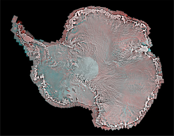
FIGURE 3.12 Radarsat-2 multipolariztion, C-band image of Antarctica collected as part of the International Polar Year. SOURCE: Courtesy of the Canadian Space Agency (for additional background information see M. Drinkwater, K. Jezek, E. Sarukhanian, and T. Mohr, IPY Satellite Observation Program, Chapter 3.1 in Understanding Earth’s Polar Challenges: International Polar Year 2007-2008, Summary Report by the IPY Joint Committee, WMO/ICSU, 2011).
shrinking sea ice cover has important consequences for future development of the Arctic. Cloud cover and the long polar night dictate the use of all-weather, day/night passive microwave radiometers for monitoring sea ice age, extent, and concentration. Older, multiyear sea ice is thicker and is structurally different from new sea ice. The lower salinity and generally rougher multiyear ice can be mapped with scatterometers and radiometers at L-band. Detailed measurements of ice extent are made using passive microwave image data at frequencies of about 18, 37, and 85 GHz. These data document the dramatic decrease in Arctic sea ice cover and the changing dates of melt onset. Visualization of northern sea ice retreat represent some of the most compelling and straightforward demonstration of the changing climate at high latitudes (Figure 3.13).
Sea ice floes in the Arctic are sufficiently large to enable motion estimates from repeat passive microwave images. Better results are obtained with increasing resolution (tens of meters) achievable
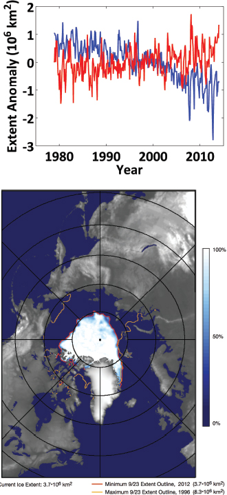
FIGURE 3.13 Top: Sea ice areal extent anomaly for the arctic (blue) and antarctic (red) from 1978 through 2013. Extent is calculated using the NASA team algorithm applied to spaceborne passive microwave data. Anomalies are deviations from the mean for the period of observations. Arctic sea ice has retreated over the period of observations. More rapid shrinkage of the ice cover began in about 2000, and that trend is continuing through the present. Conversely, Antarctic sea ice is slowly expanding over the Southern Ocean. Differences in the two trends can be attributed in part to the distinct geographies of the north and south polar regions. Nevertheless, sustained retreat of the northern ice pack is a clear indication of a warming Arctic. Bottom: Sea ice extent around the summer minimum, on September 23, 2012, from SSM/I and historical extent on the same day in 1996 from SSM/I and SMMR. SOURCE: Top: Data were provided by the National Snow and Ice Data Center; image generated by Kenneth Jezek, Ohio State University. Bottom: Courtesy of Robert Gersten and Josefino Comiso, NASA Goddard Space Flight Center.
with C-band SAR (ERS-1 and -2, Radarsat-1 and -2, and Sentinal-1). Similar to ice sheets, a net flux of sea ice across the ocean can be computed given the motion results and an estimate of ice thickness. Ice thickness is presently obtained by computing the ice surface elevation-above-sea-level as measured by Cyrosat-2 and earlier radar altimeters. Snow layer thickness obtained using airborne radars operating at 5 GHz with a 6 MHz bandwidth provides key information about insulating snow layer. Most recently, ESA SMOS L-band emission data have also been used to compute sea ice thickness.
Icebergs are a measure of the ice lost from glaciers and ice sheets by calving at the ice margin. They also represent obvious hazards to navigation. The largest (tens of kilometers) icebergs formed from long fractures through Antarctic ice shelves can be tracked with passive microwave imagers (such as SSM/I using the 18 and 37 GHz channels). Smaller icebergs can be identified and tracked with C-band SAR (such as Radarsat-1 and -2).
Seasonal snow cover plays an important role in regional hydrology and water resource management. Rapid melting of the seasonal snow pack can result in catastrophic flooding. The bright snow surface also serves as an effective mirror for returning incoming solar radiation back into space thus modulating the planetary heat budget.
Snow thickness and, indirectly, the mass of snow are key variables for estimating the volume of water available in a reservoir and potentially releasable as runoff. The most successful techniques to date have relied on microwave-based algorithms. One approach for estimating snow thickness is to difference 19 and 37 GHz brightness temperature data that along with a proportionality constant yields an estimate of the snow thickness. The algorithm is based on the fact that 19 GHz radiation tends to minimize variations in ground temperature because it is less affected by the snow pack. The 37 GHz radiation is strongly scattered by the snow grains, and brightness temperature at this frequency decreases rapidly with snow thickness/snow water equivalent.
Information about the seasonal onset of snow melt is important in river discharge and glacier mass balance studies. It can be obtained from microwave data. A few percent increase in the amount of free water in the snow pack causes the snow emissivity to approach unity, resulting in a dramatic increase in passive microwave brightness temperature. This fact has been successfully used to track the annual melt extent on the ice sheets and also to track the springtime melt progression across the Arctic. Higher resolution estimates of melt extent can be obtained with scatterometer and SAR data. These data generally show an earlier springtime date for the beginning of melt onset and a later date for the fall freeze.
Lake and river ice form seasonally at mid- and high-latitudes and high elevations. River ice forms under the flow of turbulent water, which governs its thickness. The combination of ice jams on rivers with increased water flow during springtime snow melt can result in catastrophic floods. The start of ice formation and the start of springtime ice breakup are proxy indicators for changes in local climate as well as impacts on the ability to navigate these waterways. On larger lakes, passive microwave radiometry is effective for monitoring lake ice growth and decay in much the same way as the technique is applied to sea ice.
Streams, rivers, and lakes of all sizes dot the landscape. Locally, ice cover observations can be made from aircraft. Regionally or globally, river and lake ice monitoring is challenging because physical dimensions (long but narrow rivers) often require high-resolution instruments such as SAR to resolve
details. Moreover, because the exact date of key processes, such as the onset of ice formation or river ice breakup are unknown, voluminous data sets are required to support large-scale studies.
Permafrost presents one of the greatest challenges for regional remote sensing technologies. The near surface active layer, the shallow zone where seasonal temperature swings allow for annual freeze and thaw, is complicated by different soil types and vegetative cover. This combination tends to hide the underlying persistently frozen ground from the usual airborne and spaceborne techniques mentioned above. SAR interferometry has been suggested as another tool that can be used to monitor terrain for slumping associated with thawing permafrost. For example, lakes and depressions left by drained lakes are densely distributed across the tundra and are diagnostic of permafrost conditions. SAR intensity images have been used to determine that most of these small lakes freeze completely to the bottom during the winter months. Airborne electrical resistivity measurements at kHz frequencies seem to offer a more direct approach to estimating active layer thickness and the presence/absence of permafrost.
Microwave remote sensing of the oceans is important both for understanding the oceans themselves (e.g., ocean circulation and currents) and for understanding the global hydrologic cycle and the impact of the oceans on weather and climate. It is also important for commercial applications such as monitoring fisheries and directing ship traffic. Passive measurements (radiometry) require measurement of weak thermal emissions. These measurements are generally performed at a primary frequency that is sensitive to the parameter of interest (e.g., 6.8 GHz for remote sensing of SST) and secondary frequencies necessary for correcting for effects such as attenuation along the propagation path and changes in emissivity of the surface due to roughness (waves). The same is true for active (radar) remote sensing of the oceans, although active sensors are somewhat more flexible because there is control of the transmitted signal. However, the signals are small and the systems often require passive measurements to correct for path delay (e.g., in measurements of ocean topography). Table 3.2 provides a list of the parameters of interest and the primary and secondary frequencies most commonly obtained by passive and active microwave sensors in space.
Both passive and active remote sensing techniques are limited by the availability of noise-free bandwidth. The signals are small, and bandwidth is needed to reduce noise (natural thermal noise). As
TABLE 3.2 Ocean Parameters of Interest and the Primary (black circles) and Secondary (open circles) Frequencies Most Commonly Obtained by Passive and Active Microwave Sensors in Space
| Parameter | Frequency of Observation (GHz) | |||||||
| 1.4 | 5.3 | 6.8 | 10.7 | 13.6 | 18.7 | 23.8 | 37.0 | |
| Passive | ||||||||
| Sea surface temperature | • | ○ | ○ | ○ | ○ | |||
| Sea surface winds | ○ | • | ○ | ○ | ||||
| Sea surface salinity | • | |||||||
| Active | ||||||||
| Surface topography | ○ | • | ○ | ○ | ○ | |||
the sensor technology improves, the potential for more accurate measurements and new applications increases. Given the limitations on available bandwidth, progress requires careful protection of the available bandwidth from encouragement by manmade RF interference (RFI).
Global maps of SST are important for predicting weather and understanding climate and climate change and for commercial applications such as fishery assessment. For example, knowledge of SST is important for modeling the coupling between ocean and atmosphere and for understanding the heat exchange across the boundary. Temperature together with salinity determines water density, and the density-driven circulation (thermohaline circulation) moves large amounts of water and heat around the globe.
Prior to the launch of the microwave imager (TMI) on the TRMM satellite in 1997, global maps of SST were produced from infrared measurements. Since then, data from passive microwave instruments on satellites such as AMSR-E, AMSR-2, Windsat, and GPM are being used to produce global maps of SST.5 The microwave measurements are not as limited by cloud cover and have proven particularly important for helping to forecast storms and for monitoring areas of persistent cloud cover. For example, this is the case in economically important areas off the coast of Washington and Oregon cannot be imaged in the infrared for weeks at a time because of such cloud cover.
Passive observations of the surface (i.e., measurement of the natural thermal radiation from the surface) respond to changes in SST with peak sensitivity to changes in temperature near 5-7 GHz (Figure 3.14). In this frequency range it is necessary to account for surface roughness (waves) and attenuation in the atmosphere. Modern microwave instruments generally use a combination of frequencies to retrieve SST: A primary channel near 6.8 GHz and channels near 10 GHz (to mitigate effects of waves); channels near 18 and 21 GHz to correct for attenuation by water vapor; and a frequency near 37 GHz to help correct for liquid water (note Figure 3.3). The frequencies of the microwave imager (GMI) on the recently launched GPM are 10.65, 18.70, 23.80, 36.50, and 89.00. These are bands with primary allocation for passive use, but they are shared with other active services. The AMSR series of satellites included a channel at 6.8 GHz better suited for measurement of SST. This channel is near the peak in sensitivity and critical for the measurement of SST. However, the 6.7-7.25 GHz band is not protected for passive use. ITU-R Footnote 5.458 recognizes its use for passive measurements over oceans and urges administrations to be mindful of such use.
The salinity of ocean water is important for understanding ocean circulation and its impact on weather and climate. Salinity, together with temperature, determines water density, which is important for understanding water circulation. Ocean circulation in turn is responsible for moving large amounts of heat around the globe with an impact on local weather and climate. Sea surface salinity is also important for understanding the global hydrologic cycle. Changes in salinity in the open ocean are an indication of the change in the balance between evaporation and precipitation. For example, Figure 3.15 shows the mean surface salinity field as observed by the NASA/CONAE Aquarius mission, which is very similar to a map of the global distribution of the difference between evaporation and precipitation. On a short timescale this is an indication of local precipitation, and on a longer timescale it provides important
_____________
5 For background information on EESS for SST, see the following: F. Wentz, C. Gentemann, D. Smith, and D. Chelton, Satellite measurements of sea surface temperature through clouds, Science 288(5467):847-850, 2000.
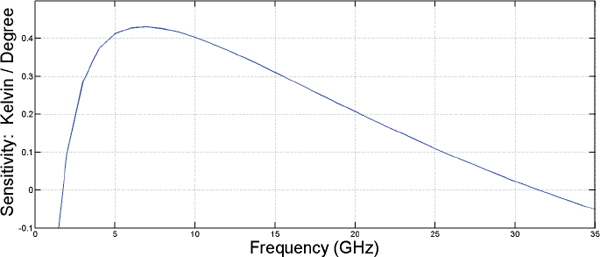
FIGURE 3.14 Sensitivity of brightness temperature to physical temperature (nadir and sea surface salinity = 30 psu). SOURCE: Courtesy of David Le Vine, NASA Goddard Space Flight Center.
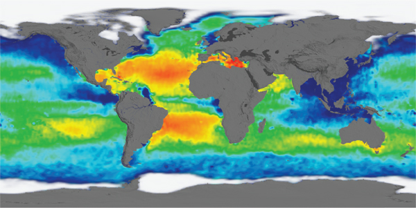
FIGURE 3.15 Remote sensing of sea surface salinity is important to improve understanding of ocean circulation and the global water cycle, and their role in climate and climate change. This image is an example of data produced by Aquarius. It shows the general features of the distribution of ocean salinity (e.g., saltier Atlantic than Pacific; and salty mid-latitudes separated by fresher water created by rain in the tropics). However, the maps are produced weekly and also show the dynamics of the salinity field including short-term changes associated with river runoff and longer term effects (e.g., seasonal and inter-annual) associated with the evolution of the mean field. SOURCE: Courtesy of the Aquarius Project; see NASA Aquarius, “Climatology Maps of Aquarius Data (V.4.0),” Gallery: Climatology, http://aquarius.umaine.edu/cgi/gal_climatology.htm.
boundary conditions for understanding ocean-atmosphere coupling. Changes in salinity in the northern latitudes (e.g., Labrador Sea and Irminger Sea) are indications of freshwater input from melting ice and can be an indicator of climate change. As important as salinity is to ocean dynamics, it is relatively poorly measured. Historically, it has been measured by ships and more recently by a system of floats and buoys (e.g., Argo floats). However, even thousands of point measurements provide poor sampling of the spatial and temporal variations in the vast oceans.
Surface salinity can be measured remotely from space by detecting changes in the natural (i.e., thermal) emission from the surface. The conductivity of seawater depends on the salt content, which changes the dielectric constant and emissivity at the surface (salty water has a higher conductivity and lower emissivity). The change is small (about 0.5 K/psu at 1.4 GHz) but is detectable with modern microwave radiometers. One issue for remote sensing is that the sensitivity is frequency dependent and decreases very rapidly (Figure 3.16). Antenna size and the ionosphere limit measurements to frequencies above about 1 GHz, and the sensitivity is too low above 2-3 GHz. Without the protected spectral window at 1.413 GHz and its radiometers, this measurement would not be practical.
Another important issue is surface roughness (waves). Wind-driven waves can cause a change in emission almost as large as that due to changes in salinity. As a result sensors such as Aquarius that are designed to monitor surface salinity globally from space, include a radar (scatterometer) to help correct for roughness. The Aquarius scatterometer operated at 1.26 GHz in a shared band is an example of combined active/passive microwave remote sensing.6 Data from both sensors are needed for an accurate measurement.
Measuring sea surface salinity also depends on ancillary information such as surface temperature, atmospheric attenuation, and knowledge of radiation from other sources (e.g., the Sun and galactic background) that are also products of microwave remote sensing and other scientific applications requiring noise-free access to the spectrum. To make these measurements (i.e., SST) requires a sensor with bands at 6.8, 10.65, 18.70, 23.80, and 36.50 (e.g., AMSR).
Winds at the ocean surface are important for weather forecasts, such as monitoring and developing warnings for storms and to provide boundary conditions in numerical weather forecast models. Information on surface winds is also used in operational applications such as predicting sea state, routing of ships, tracking buoys, and supporting ocean-based defense operations (navy operations).
Surface winds can be monitored with passive microwave instruments because of the coupling of winds to waves and the effect of waves on the emissivity of the surface. In the microwave spectrum the sensitivity to surface roughness increases with frequency until about 10 GHz, after which it is roughly constant. Passive measurement of surface winds generally requires several frequencies. For example, Windsat uses channels at 6.8, 10.7, 18.7, 23.8, and 37.0 GHz. The channel at 6.8 GHz helps to mitigate the effects of SST, and the channels at 18.7 and 23.8 GHz to help correct for attenuation in atmosphere. Instruments scanning in azimuthal directions can also provide wind direction because of differences in along-wind and crosswind emissivity and dependence on polarization.
Surface winds can also be monitored with active microwave instruments. Backscatter from instruments such as NSCAT, QuickSCAT, and RapidSCAT, which operate near 13.5 GHz, responds to surface roughness and, by looking in multiple directions, produce wind speed and direction. Winds have also been retrieved successfully with scatterometers operating at L-band (1.26 GHz). Active/passive combinations
_____________
6 For technical information on EESS for measuring ocean salinity, see the following: D.M. Le Vine, G.S.E. Lagerloef, and S. Torrusio, Aquarius and remote sensing of sea surface salinity from space, Proceedings of the IEEE 98(5):688-703, 2010.
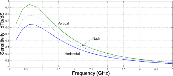
FIGURE 3.16 The sensitivity of brightness temperature of an ideal ocean surface (no waves) to changes in salinity as a function of frequency for nadir (broken curve) and at 40 degrees (solid curves). The calculations are for a surface with sea surface salinity = 35 psu and sea surface temperature = 20°C. SOURCE: Courtesy of David Le Vine, NASA Goddard Space Flight Center.
have also been employed (e.g., Aquarius and SMAP) where the radar (1.26 GHz) provides a correction for roughness and an independent estimate roughness or winds needed by the passive sensor (1.41 GHz).
Both active (radar) and passive (radiometer) measurements require highly sensitive instruments operating in a noise-free environment. However, the bands available are generally shared with other services (e.g., the radar band at 1.26 GHz).
Details of the surface of the ocean provide information for several important ocean, weather, and climate applications. For example, roughness is related to sea state and surface winds. Sea level (e.g., height and topography) changes with water temperature, and variations in sea level provide estimates of the upper-level heat content. Water velocity is also related to surface height (geostrophic current), and maps of the surface topography can be used to study ocean circulation.
Microwave radar altimeters in orbit are used to provide global maps of the ocean surface to support these applications. The altimeter is essentially a short-pulse, nadir-looking radar. By looking at the shape of the returned signal and the travel time, it is possible to infer information about the sea surface topography (e.g., height and roughness). Radar altimeters have been operating in space since the early 1990s including Topex/Poseidon, Jason-1, and the Ocean Surface Topography Mission (OSTM) on Jason-2. These instruments operate at 13.6 GHz with a channel at 5.3 GHz and also include a radiometer to help correct for path delay. Typically, radiometer channels are at 18.7, 23.8, and 34.0 GHz. After 20 years of experience in orbit, the modern science objectives for spaceborne altimetry are impressive:
- Estimates of the transport of heat, water mass, nutrients, and salt by the oceans;
- Increased understanding of ocean circulation and how it changes with time;
- Estimates of significant wave height and wind speed;
- Improved knowledge of ocean tides and open-ocean tide models;
- Improved forecasting of climatic events like El Niño;
- Improved understanding of the variation of global mean sea level and its relation to global and climate change.
The radar altimeter also has potential for applications over land, for example in monitoring changes in ice cover and mapping properties of the surface. But the measurements require high accuracy and operating in shared and/or partially protected frequency bands raises the problem of interference.
The science of the solid Earth and biosphere covers a variety of applications related to Earth’s surfaces and those systems that inhabit it. For these applications the RF spectrum is used either passively, to observe variations in black body radiation and target emissivity (whose signature is regulated by moisture content), or actively, which allows for measures of relative reflected power, signal phase, and time of flight to be made and related to physical characteristics of the target.
In many of these applications, access to specific frequencies is less important than having some degree of frequency (and wavelength) diversity because remote sensing of terrestrial targets is most sensitive to the target’s broad structural and shape characteristics, as well as dielectric and surface roughness contrasts with respect to surrounding areas. In all, the sensitivity to these characteristics is maximized when the physical scale of the variations is similar to the observing wavelength.
For active systems, bandwidth is used to better determine the target range. RFI-free bandwidths permit passive systems to achieve a more accurate thermal/emissivity signature for the target being observed.
Because of the non-frequency specific nature of the described applications, RF spectrum requirements occur at octave-level intervals. Historically, such spectrum, often coincident with atmospheric windows, has been available for these systems The frequencies where most solid Earth and biosphere measurements are obtained are listed in Table 3.3.
The long history of observations made in these bands allows the temporal evolution of the phenomena to be observed. Observation systems themselves have also benefited from historical resources,
TABLE 3.3 Frequencies Where Most of the Active Science-Application Systems Operate for Studying the Solid Earth and Biosphere
| Band Designation | Passive Spectra | Active Spectra | Role | |||||
| P-band | 432-438 MHz | Biomass imaging, root zone soil moisture, below-canopy surface topography | ||||||
| L-band | 1.42 GHz | 1215-1300 MHz | Biomass imaging, forest change detection, surface motion and subsidence | |||||
| S-band | 3100-3300 MHz | Agricultural monitoring | ||||||
| C-band | 5250-5570 MHz | Agricultural monitoring, surface change detection | ||||||
| X-band | 8550-8650 MHz, 9300-9900 MHz | Vegetation and elevation mapping | ||||||
| Ka-band | 35.5-36 GHz | Surface water and elevation mapping | ||||||
such as standardized parts and existing infrastructure. The development of technology and observational capabilities in these areas relies on a stable and predictable RF spectral environment.
A more in-depth discussion for three areas of solid Earth and the biosphere is presented below: (1) surface dynamics and deformation, (2) agricultural productivity, and (3) terrestrial carbon storage. Indeed, there are many more applications than this short list can provide, or that can be discussed in the space provided here. In each however, the use of the RF spectrum is often divided up into active and passive applications, the details of which are related to the configuration of the sensing system and the physics of the electromagnetic interaction that is being exploited to extract physical parameters of interest.
3.6.1 Surface Dynamics and Deformation
Earth’s solid surface is often undergoing change. This change occurs through incremental events, such as land subsidence and soil erosion/deposition, or changes driven by drastic and short-lived events such as earthquakes, volcanic eruptions, and landslides.7
The types of remote sensing that are applied to these types of changes often make use of the coherent nature of electromagnetic signals, especially in the microwave region extending on the low-frequency radar side from L-band up to X-band. In this context, low-frequency signals have the advantage of penetrating through ground cover and reflecting primarily from the solid surface, whereas higher frequency signals have the advantage of increased sensitivity to change, because of the wavelength-dependent nature for the coherent detection of this change. At the low-frequency extreme of observation (e.g., P-band), the interaction of the ionosphere with the signal causes variations in the signal phase that can be difficult to extract from the desired surface deformation signature. At the higher frequency extremes, X-band and above, physical changes in the surface geometry on the order of a wavelength and electromagnetic characteristics (e.g., dielectric changes) will cause the signal to decorrelate over time, and similarly obscure the sought-after deformation signature.
Airborne and especially spaceborne remote sensing play a role in solid Earth science because of their ability to make repeated measurements over long time periods. Often these measurements are made in the high-resolution configuration of SAR, which allows for three-dimensional maps to be made of the deformation. The resolution of SAR systems is dictated by the signal bandwidth (typically on the range of 10 MHz to 100 MHz) and the size of the antenna aperture in the along-track direction of the flight platform. If interference occurs in this bandwidth, then it can be dealt with through filtering of the signal in the frequency domain. However, because of the high sensitivity of deformation measurements to signal phase, the implementation of these filters has a deleterious effect on the deformation measure, and for that reason, notch-filters (those with a steep frequency response) are generally avoided.
3.6.2 Agricultural Productivity
Agricultural production is important for human health and safety. Agricultural productivity changes from year to year as the local environment changes and in response to government policies, so it is important to track these changes. While much of this monitoring takes place through direct interaction between the sources of production and government organizations such as the U.S. Department of Agri-
_____________
7 For background regarding EESS in understanding surface dynamics and deformation, see the following: D. Massonnet and K.L. Feigl, Radar interferometry and its application to changes in the Earth’s surface, Reviews of Geophysics 36(4):441-500, 1998.
culture, the factors governing production, such as soil moisture and water availability, and the outputs of the production as they manifest themselves in crop health monitoring, are important components as well.
Both passive and active remote sensing are used in this context for monitoring changes in soil moisture and groundcover. Employing passive remote sensing to measure soil moisture requires the use of C-band frequencies and below in order for the signal to penetrate through the crop and directly sense the soil surface. Measurements such as these, made from either spaceborne or airborne platforms, use real-aperture antennas and have resolutions ranging from tens of meters up to tens of kilometers. For this reason, moisture measurements are made over large regions, consisting of many crops and land management practices.
Active remote sensing of agriculture crops makes use of the improved resolution (along- and cross-track) that these systems can achieve with an active signal.8 High-frequency observations (e.g., X-band), sensitive to small plant structures and the upper part of an agricultural canopy, are important for monitoring early growth and estimating water resources available to the sun-gathering components of the canopy. Lower frequency signals (C-, S-, and L-band) are used for estimating bulk characteristics of the canopy. Calibrated ratios of power between these frequencies (which differentiate crop type and crop density) are important factors in estimating crop yield and for detecting the early detection of crop disease and drought. The lowest frequency observations of crops (L- or P-band), when combined with estimates of surface roughness, canopy height, and time-series measurements, can be used for making high-resolution estimates of soil moisture, an important component in overall crop health. Thus, because farming practices vary widely around the world, these applications benefit greatly from high-bandwidth and high-resolution observations.
3.6.3 Terrestrial Carbon Storage
Earth’s vegetation canopy, or biomass, is a significant component of the global carbon inventory and a source of its greatest uncertainty. It is also a major contributor to the net long-wave/short-wave albedo of the planet and hence to Earth’s energy balance and temperature. For these reasons, climate change can both be affected by and can itself affect the global distribution of biomass.
The ability to perform comprehensive inventories of biomass from space is recognized as a critical step toward modeling and understanding Earth’s climate system. Passive microwave observations operating in all of the primary atmospheric window channels between 1.4 and 90 GHz are valuable for monitoring the full range of vegetation canopy water content found in nature and are complementary to optical and synthetic aperture radar techniques. Improved techniques for biomass estimation using passive microwave methods are continuously being developed (Figure 3.17).
Active sensing of the vegetation canopy makes use of the volume scattering component of the canopy and is used as a signature for the height of the canopy and to estimate the amount of above-ground biomass stored in the vegetation.9 Such measures are important for characterizing animal and plant habitats, for detecting natural or manmade changes in the land cover, and for better understanding the global carbon budget.
_____________
8 For background in active EESS in agricultural monitoring, see the following: J.M. Lopez-Sanchez and J.D. Ballester-Berman, Potentials of polarimetric SAR interferometry for agriculture monitoring, Radiation Science 44, 2010; H. McNairn and B. Brisco, The application of C-band polarimetric SAR for agriculture: A review, Canadian Journal of Remote Sensing 30(3):525-542, 2004.
9 For background on active EESS for forest studies, see the following: R. Ahmed, P. Siqueira, S. Hensley, B. Chapman, and K. Bergen. A survey of temporal decorrelation from spaceborne L-Band repeat-pass InSAR, Remote Sensing of Environment 115(11):2887-2896, 2011.
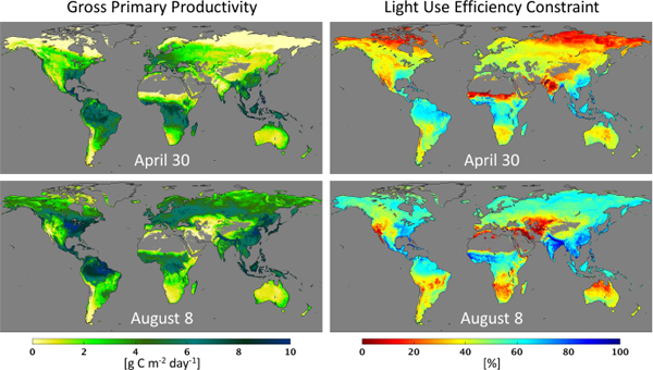
FIGURE 3.17 Vegetation gross primary production (GPP, g C m-2 day-1) and the proportion (%) of estimated daily GPP to potential growth from the NASA SMAP (Soil Moisture Active Passive) mission Level 4 Carbon (L4_C) product; GPP defines the photosynthetic rate of green plants and conversion of atmosphere carbon dioxide (CO2) to plant biomass, including forest, rangeland, and agricultural productivity. The proportional reduction in daily GPP shows where environmental conditions are less than optimal for plant growth (including areas with frozen temperatures and low soil moisture levels determined from SMAP active and passive microwave remote sensing; observed GPP reduction map ranges from optimal (100%) to fully constrained (0%) growth conditions). The L4_C results are shown for April 13 and May 25, 2015, and capture the northerly migration of spring green-up and associated onset of the growing season across the Northern Hemisphere; the onset of GPP in spring coincides with a seasonal shift to favorable growth conditions from thawing temperatures and relatively abundant soil moisture conditions from April to May. Strong GPP reductions from potential growth conditions are also observed over many (red shaded) areas, including the African Sahel, northern India and southwest United States, stemming from regional drought. SOURCE: Courtesy of John Kimball and Lucas Jones, University of Montana.
The physical mechanisms for this active sensing typically take on one of three forms. These are (1) measure of the frequency-dependent radar backscattered power, (2) measure of the polarimetric scattering characteristics of the target, and (3) use of single- and repeat-pass SAR interferometry for determining the target volume scattering characteristics, which can be related to the vegetation height and vertical density profile. In all of these applications, the frequency determines the depth of penetration into the vegetation canopy; different frequencies (or wavelengths) are chosen such that they are primarily sensitive to the upper or lower parts of the vegetation layer. Frequencies that are of primary interest for this application range from P-band up to X-band. Multiple-frequency observations and their ratios are used to remove systematic variations that occur due to weather, moisture, and topographic conditions, and assess the underlying structural components of the vegetation that are of interest.


