
The analytic approach taken to arrive at an estimate of obesity prevalence or trend is determined by a number of factors, including the intent of the specific analysis, the quality control measures taken during data collection, the study design from which the data were derived, and the amount of data available. A range of options exist to analyze the data and to present the results. In its review of the evidence, the committee identified various aspects of the analytic approaches used in published reports that have implications for interpreting results. Some analytic approaches, such as the reference population selected to classify body mass index (BMI), specifically pertain to the assessment of obesity among children, adolescents, and young adults. Other interpretive considerations are fundamental principles of epidemiology and statistics and are widely applicable to any assessment of prevalence or trends. Both are integral to a thorough consideration and informed interpretation of results.
This chapter highlights key considerations that extend across the broad range of published reports on obesity prevalence and trends. Throughout, analytic approaches will be described. These descriptions are not intended to provide detailed guidance on how to perform the specific procedures, but rather are included to contextualize the consideration, especially for those who do not have advanced understanding of statistics and epidemiology. The committee acknowledges that other analytic procedures and considerations exist beyond those presented here.
This chapter contains terms and phrases that have the potential to be used or interpreted in multiple ways. For clarity, the committee’s definitions are as follows (a full glossary can be found in Appendix A):
- “Analytic approach” encompasses both the preparation of data for analysis and the statistical analyses themselves.
- “Statistical analysis” or “statistical approach” will specifically refer to the analytic procedures that result in an estimate of obesity prevalence or trend.
- “Estimate of obesity prevalence or trend,” or the term “estimate,” describes a statistic about the proportion or number of individuals affected with obesity at one point in time (prevalence) or over time (trend).
- “Change” refers to the difference between two points in time, and “trend” refers to a difference over three or more points in time.
- “Investigators” describe those who perform the analyses.
THE PUBLISHED REPORT’S STATEMENT OF PURPOSE
A published report’s stated purpose provides a link between the data source and the analytic procedure. It also can provide initial insight into the type of findings to be presented (e.g., prevalence, change, trends). The committee identified recurring themes in the stated purposes across a wide variety of published reports (see Table 5-1). This list of themes is not exhaustive, but it illustrates that a range of purposes can fall under the purview of a “report on obesity prevalence or trends.” Although some analytic approaches are common across all published reports (e.g., classification of obesity status), the statistical analyses performed are tailored to the specific research question or defined set of questions being asked of the data.
PREPARATION OF THE DATA FOR ANALYSIS
Published reports commonly describe the steps taken to prepare the data for statistical analysis. Some data preparation procedures are specific to an evaluation of obesity, especially when the sample includes children, adolescents, and young adults. Other data preparation procedures are general and rooted in the principles of epidemiologic research and statistical analyses. The extent to which these specific and general procedures are performed can vary.
The committee identified three key aspects of data preparation that can affect the interpretation of findings presented in a published report on obesity prevalence and trends. These include: the approach to obesity classification, identification and handling of biologically implausible values (BIVs), and representativeness of the sample.
TABLE 5-1 Potential Advantages and Disadvantages of Published Reports on Obesity Prevalence and Trends, by Thematic Characterization of the Report’s Statement of Purposea
| Purpose | Potential Advantagesb | Potential Disadvantagesb |
|---|---|---|
| Report obesity prevalence in a single population |
As the primary objective, the estimates are typically easy to identify. |
Describes only one point in time. Does not provide insight into incidence or variations over time. |
| Compare obesity prevalence and trends of different population groups |
Provides insight into how different groups are affected. |
Subgroupings can rapidly become small in size, limiting meaningful comparisons. Time frame(s) selected affects results, interpretation of findings. |
| Compare obesity prevalence estimates between multiple locations, regions, or states |
Helps elucidate how prevalence estimates relate to each other geographically. |
May not account for all differences between locations that can affect estimates of obesity prevalence. Jurisdictions of interest to the end user may not have comparable data or be included in the report. |
| Compare an estimate to a national statistic |
National estimates provide a benchmark. |
Groups will inherently fall above and below the national estimate because it represents a central tendency. |
| Assess change in prevalence after implementation of a policy or initiativec |
Provides a broad picture of the status before and after a population-wide change. |
Causality cannot be established. There are limits to what can be controlled for in the analysis. |
| Assess how a group of individuals change over time |
Assesses intrapersonal change or trajectories. |
Attrition is likely, which can limit generalizability. Results highly contingent on time period assessed, with shorter trends typically being less stable than longer ones. |
a The list is not exhaustive and categories are not mutually exclusive.
b The potential advantages and disadvantages are contingent on the population assessed, the methodology employed, the analytic approach, and the end user seeking to apply such information. Population and methodologic considerations are discussed in Chapter 3. The analytic considerations are more fully explored in this chapter, while considerations related to end users are discussed in Chapter 6.
c Considered natural experiments, which are observational rather than interventional in design.
Obesity Classification for Children, Adolescents, and Young Adults
As described in Chapter 2, obesity status must be operationalized into a metric that can be categorized. BMI is the predominant measure used to classify obesity status. Although the adult cut point for obesity classification of >30 kg/m2 applies to both sexes regardless of age, the cut point for children is determined by comparing BMI to a reference population. The 2000 Centers for Disease Control and Prevention (CDC) sex-specific BMI-for-age growth charts are the predominant reference used for U.S. children, ages 2 years and older. However, other BMI-for-age references appear in published reports, specifically the International Obesity Task Force (IOTF) cut points and the World Health Organizations (WHO) growth standards and charts. The following sections describe the utility and comparability of these reference populations and Table 5-2 summarizes them. Other growth references exist, but because they are not typically used in published reports on U.S. populations, they are not included in this section.
Growth References for Classifying Obesity Status
2000 CDC BMI-for-Age Growth Charts The 2000 CDC sex-specific BMI-for-age growth charts are designed for individuals ages 2 to 20 years (see Figure 2-1 for an example) (Kuczmarski et al., 2000). Data used to develop the BMI-for-age growth charts came from the National Health Examination Survey (NHES) II (1963-1965), NHES III (1966-1970), National Health and Nutrition Examination Survey (NHANES) I (1971-1974), and NHANES II (1976-1980). Data from NHANES III (1988-1994) were used only for children younger than age 6 years because obesity prevalence was substantially higher in this NHANES cycle than the previous cycles and inclusion would have shifted cut off points for obesity classification (Kuczmarski et al., 2000). Smoothed percentiles are assigned throughout the distribution of each of the sex-specific curves. The percentiles serve as the basis for classification of weight status. A child with a BMI at or above the 95th percentile for age and sex is classified as having obesity (see Box 2-3 for discussion about recent shifts in nomenclature).
Using the growth charts to classify obesity status has two interpretive considerations. First, like all reference population-based classification approaches, the 2000 CDC BMI-for-age growth charts represent the distribution of BMIs that existed within the source population, which consisted of nationally representative samples of U.S. children from the 1960s through the 1980s. The children who were included were not selected based on health criteria, and as such, the distribution describes only the distribution as it existed and does not necessarily reflect optimal growth. Second, by definition, 5 percent of the children whose data were used to develop the
TABLE 5-2 Summary of the 2000 CDC BMI-for-Age Growth Charts, the IOTF Cut Points, the WHO Growth Standard, and the WHO Growth Reference
| Growth Reference | Source Populationa | Cut Point to Classify Obesity | Age Aligned with Adult Cut Pointb |
|---|---|---|---|
| CDC |
Nationally representative |
≥95th percentile cross-sectional samples of U.S. children, adolescents, and young adultsd |
Males: 19.3 years |
| IOTF |
Representative samples from six locations |
Centile corresponding to a BMI of 30 kg/m2 at age 18 years applied throughout the distribution |
18 years |
| WHO, growth standard | MGRS |
+2 standard deviations |
N/A |
| WHO, growth reference |
1977 National Center for Health Statistics/WHO growth reference, merged with the MGRS data |
+2 standard deviations |
19 years (approximately) |
NOTE: CDC, Centers for Disease Control and Prevention; IOTF, International Obesity Task Force; MGRS, Multicentre Growth Reference Study; N/A, not applicable; WHO, World Health Organization.
a Only pertains to the BMI-for-age growth charts.
b Age in which the growth reference crosses 30 kg/m2.
c The potential advantages and disadvantages are contingent on the population assessed, the methodology employed, the analytic approach, and the end user seeking to apply such
BMI-for-age growth chart would have exceeded the 95th percentile cut off point (Ogden, 2015). Together, these considerations emphasize the statistical principles underlying the classification of obesity status using the growth chart approach.
The 2000 CDC BMI-for-age growth charts have several practical advantages. One advantage, as nationally representative growth references, is that their use is pervasive in the U.S. published literature, which facilitates comparability across reports. Another advantage is that the CDC provides tools, including a Web-based calculator (CDC, 2015a) and a download-able spreadsheet (CDC, 2015c), that calculate BMI percentile (and thereby obesity status) when height, weight, date of measurement, and date of birth are entered.
| Potential Advantagesc | Potential Disadvantagesc | Interpretations |
|---|---|---|
|
Pervasive in the literature. Source data were nationally representative of U.S. population. |
Does not describe optimal growth. Not directly aligned with the adult cutoff. |
Comparison to a distribution of previous nationally representative U.S. samples. |
|
Provides continuity with adult obesity cut point. Can be used internationally. |
Does not describe optimal growth. |
Comparison to distribution of six previous representative international samples. |
|
Source population represents optimal growth. Can be used internationally. |
Available only for young children. |
Comparison to young children believed to exemplify optimal growth. |
|
Aligned with the age 0 to 5 year growth standard for continuity. Can be used internationally. |
Does not describe optimal growth. |
Comparison to a distribution of previous nationally representative U.S. samples. |
information. Population and methodologic considerations are discussed in Chapter 3. The analytic considerations are more fully explored in this chapter, while considerations related to end users are discussed in Chapter 6.
d Data from the National Health Examination Survey (NHES) II (1963-1965), NHES III (1966-1970), National Health and Nutrition Examination Survey (NHANES) I (1971-1974), and NHANES II (1976-1980). Data from NHANES III (1988-1994) were used only for children younger than age 6 years (Kuczmarski et al., 2000).
The use of the 2000 CDC BMI-for-age growth charts also has some limitations. The age in which an individual transitions from the growth charts to the adult cut point for obesity is inconsistent across reports. Some investigators use the growth charts for individuals through age 19 years (Gee et al., 2013; Ogden et al., 2014), while others use the 30 kg/m2 cut point for all individuals ages 18 years and older (Hinkle et al., 2012). The 95th percentiles on the growth charts do not correspond to a BMI of 30 kg/m2 at either age for either sex. On the female growth chart, the 95th percentile crosses a BMI of 30 kg/m2 at age 17.5 years and corresponds to BMIs higher than 30 kg/m2 thereafter. For females aged 17.5 to 20.0 years, use of the growth chart has the potential to result in a lower obesity prevalence than a prevalence based on the 30 kg/m2 cut point. For males,
the 95th percentile does not cross the adult BMI cutoff until 19.3 years of age. Before this age, use of the growth chart has the potential to result in a higher obesity prevalence compared to a prevalence based in the 30 kg/m2 cut point. After age 19.3 years, where the 95th percentile corresponds to a BMI greater than 30 kg/m2, obesity prevalence based in the growth charts has the potential to be lower than prevalence based on the adult cut point. To account for these differences, some investigators classify adolescents and young adults as having obesity if their BMI is either ≥95th percentile or ≥30 kg/m2, whichever corresponded to a lower BMI (Benson et al., 2009, 2011; Freedman et al., 2012; Robinson et al., 2013). Although the use of the adult criterion in conjunction with the growth charts is one method for handling the discrepancy between the different approaches, it has the potential to classify more individuals as having obesity than the growth charts alone. Although rarely reported in the published literature, the extent to which the estimate of obesity prevalence changes with the inclusion and exclusion of the 30 kg/m2 criterion for an analytic sample provides evidence of its utility and need for a given population.
IOTF BMI Cut Points Although the IOTF BMI cut points are not as common as the 2000 CDC BMI-for-age growth charts in the published literature, they have been used in reports on U.S. children and adolescent populations (Rodriguez-Colon et al., 2011; von Hippel and Nahhas, 2013; Williamson et al., 2011). The sex-specific IOTF cut points are based on cross-sectional, nationally representative data from six different countries from various years: Brazil (data from 1989), Great Britain (data from 1978-1993), Hong Kong (data from 1993), the Netherlands (data from 1980), Singapore (data from 1993), and the United States (data from 1963-1980) (Cole et al., 2000). The U.S. data included in the IOTF analyses are the same data that were used to develop the 2000 CDC BMI-for-age growth charts (i.e., NHES II, NHES III, NHANES I, and NHANES II). The IOTF BMI cut points, however, are based on pooled nationally representative data from different parts of the world, and are therefore intended for international use.
The IOTF BMI cut points provide classification continuity from childhood through adulthood. By design, a BMI of 30 kg/m2 at age 18 years for both sexes corresponds to being classified as having obesity (Cole et al., 2000). The centile associated with this cut point was then applied to the rest of the BMI distribution to establish obesity and other weight classification cut points throughout childhood and adolescence (Cole et al., 2000). These cut points also have been updated so that they can be expressed as a centile or standard deviation score (z-score; see Box 5-3 for description) (Cole and Lobstein, 2012).
Although the IOTF cut points have international applications and allow for a seamless transition to the adult cut point for obesity, the inter-
pretation of obesity classification is still rooted in the source populations of the data. Like the 2000 CDC BMI-for-age growth charts, the IOTF BMI distributions were derived from nationally representative samples—in this instance, six international populations—and therefore do not necessarily describe optimal growth. Thus, obesity classification using the IOTF is a comparison of a BMI to the distribution of children’s BMIs that existed at the time points the data were collected from various international locations.
WHO Growth Standards and Growth Charts The WHO developed growth standards for children 0 to 5 years of age and growth references for children 5 to 19 years of age. A growth reference and a growth standard differ in attributes of the source population. A reference describes the typical physical development found in a population but does not necessarily provide insight into what deviations from typical values mean. A standard, in contrast, describes the development of children who are believed to exemplify optimal growth and “may be considered as prescriptive or normative references” (de Onis, 2004). The CDC endorses the use of a modified version of the WHO growth charts for U.S. children younger than age 2 years (Grummer-Strawn et al., 2010) but recommends use of the 2000 CDC growth charts thereafter (CDC, 2010). Accordingly, use of the WHO growth standards and charts are not particularly common in reports on obesity prevalence and trends among U.S. population groups.
Data for the growth standards for children ages 0 to 5 years came from the Multicentre Growth Reference Study (MGRS), a population-based, international effort that sought to describe optimal growth of children (de Onis, 2004). It consisted of a longitudinal assessment of children from birth to 24 months of age and a cross-sectional assessment of children ages 18 to 72 months. Participants were recruited from six study sites (Accra, Ghana; Davis, California, United States; Muscat, Oman; New Delhi, India; Oslo, Norway; and Pelotas, Brazil) and met strict inclusion criteria, in an effort to capture the growth status and growth trajectory of children with optimal health, nutrition, and environmental exposures. The strict inclusion criteria allowed for an assessment of comparability of growth across the locations, in which racial and ethnic compositions of the assessed populations and cultural practices differed. For linear growth, approximately 3 percent of the variability was attributed to location, while 70 percent was attributed to individual variation (WHO MGRS, 2006). As described in Box 5-1, the limited variability in growth that can be attributed to racial, ethnic, or international geographic location among young children provides evidence to support the use of a single reference population across various racial and ethnic groups, with considerations for environmental and socioeconomic status.
For the growth reference for children and adolescents ages 5 to 19 years, data from the ages 0 to 5 year growth standards were merged with data used to develop the 1977 National Center for Health Statistics (NCHS)/WHO growth references, which were from NHES II, NHES III, and NHANES I (de Onis et al., 2007). The reference population for the WHO growth charts, therefore, includes much, but not all, of the data used to develop the 2000 CDC BMI-for-age growth charts. The WHO growth references are aligned with the age 0 to 5 years growth standards, providing continuity as children younger than age 5 years transition to the growth reference for those ages 5 to 19 years.
For the WHO growth charts, a child with a BMI exceeding +2 standard deviations (approximately the 98th percentile) is classified as having obesity. The +2 standard deviation cut point for both sexes at age 19 years closely corresponds to the adult cut point for obesity (29.7 kg/m2 versus 30 kg/m2, respectively) (de Onis et al., 2007).
Comparability of Growth References for Obesity Classification
The CDC, IOTF, and WHO growth references each used U.S. nationally representative data in their development, alone or in combination with other data sources. The reference populations and associated BMI-for-age
distributions differ across the growth charts. The selected cut points used to categorize obesity status also differ. As a result, obesity prevalence can vary depending on which reference is used. For school-aged children, for example, the IOTF cut points are more closely aligned with the CDC’s 97th percentile than the 95th percentile (Freedman et al., 2011). Because IOTF cut points correspond to a higher threshold, obesity prevalence calculated using the IOTF will be lower than prevalence based on CDC growth charts (Freedman et al., 2011; Lang et al., 2011). In contrast, the WHO and CDC obesity classification approaches have been noted to yield estimates of obesity prevalence relatively aligned with each other, although variation exists. Both Maalouf-Manasseh et al. (2011) and Mei et al. (2008), for example, reported higher obesity prevalence in populations younger than age 5 years using the WHO growth charts compared to the CDC. Thus, obesity prevalence estimates using the different reference populations are not interchangeable.
Alternative Obesity Classification Approach
Some published reports do not use any of the aforementioned reference populations and instead use novel or different criteria for obesity classification. Some published reports, for example, are based on publicly available data in which the alternative classification criteria are embedded in the data collection or reporting system from which the data were derived (see Box 5-2 for an illustrative example). Other reports have the primary purpose of determining the utility of an alternative obesity classification criterion. Reports of this nature have the potential to alter how obesity is determined and described, and thereby serve an important research niche. However, use of such reports for the purposes of determining obesity prevalence and trends can be challenging. The statistic must be interpreted in context of the criteria used to classify the data and can be limited in its comparability to existing statistics.
Summary of Considerations Related to Obesity Status Classification
- Different reference populations exist. The CDC, IOTF, and WHO each provide different reference population to which BMIs can be compared.
- Interpretation of obesity classification is embedded in the design of the growth charts. The three reference populations describe the distribution of BMIs as they existed within the source population. The obesity cut points selected are statistically derived from those distributions.
- Obesity prevalence is contingent on the reference population selected. Because the CDC, IOTF, and WHO cut points were developed using
different source data, the distributions and associated obesity cut points are not identical. Obesity prevalence is typically lower when using the IOTF cut points, compared to CDC growth charts.
Biologically Implausible Values
Extreme values for height, weight, and BMI occur in datasets. The identification and handling of these BIVs is a data processing procedure
that is common, although not universal, among reports on obesity prevalence and trends. A BIV may represent an error in measurement or data entry and can exist on both ends of the spectrum—that is, values can be implausibly high or implausibly low. Both inclusion of BIV data that are errors and exclusion of BIV that are legitimate data points can affect an obesity prevalence or trend estimate. Because the purpose of identifying BIVs is to locate extreme values in the data, BIV criteria are often based on evaluation of growth reference z-scores rather than percentiles (Flegal and Ogden, 2011) (see Box 5-3).
To identify data that qualify as BIVs, investigators establish a range of plausible values. Data falling outside of the plausible range are classified as BIVs. BMI is an index of height and weight, and as such, BIVs can exist in height, weight, and BMI data. Lawman et al. (2015), however, note that not all large-scale epidemiologic studies report evaluating BIV in height, weight, and BMI data—some only report evaluating extremes in BMI data. The following provides an overview of the different types of BIV criteria that exist and how BIVs have been handled.
Types of BIV Criteria
The criteria used to identify BIVs can be flexible or fixed (CDC, 2016b; WHO, 1995). Flexible BIV criteria are constructed around the observed
mean of the collected data for a particular study. This approach is particularly useful when the sample’s distribution is shifted because it allows the acceptable range of deviation to be wider. Fixed BIV criteria, in contrast, are absolute cutoffs that are independent of the collected data and are based on the reference population. Fixed BIV criteria recommended by a 1995 WHO expert committee are presented in Table 5-3. Using fixed data is useful when the assessed population’s mean z-score, as compared to the reference population, is relatively close to zero. Fixed criteria can be adapted to account for skewed population distributions. If an assessed population BMI-for-age distribution is skewed, as was the case for Pan et al. (2012), a higher cut point for implausible values may be used (e.g., +8 standard deviations instead of +5) (CDC, 2015d).
The fixed criteria presented in Table 5-3 were released before the development of the BMI-for-age growth charts. When the 2000 CDC BMI-for-age growth charts were developed, skewness in the distribution was handled in such a way that extreme values converge to high but still plausible z-scores (CDC, 2002, 2016b; Flegal and Cole, 2013). As such, extrapolation beyond the 97th percentile on the growth charts should be carried out with caution (CDC, 2002; Flegal and Cole, 2013; Flegal et al., 2009). To overcome this limitation, the CDC has developed a statistical program that calculates modified age- and sex-specific z-scores that can be used for BIV identification (CDC, 2015d).
As described in a review of BIV criteria used in large epidemiologic studies, not all reports use the same approach to identifying BIVs related to height, weight, or BMI (Lawman et al., 2015). Instead, BIV criteria have been based on z-scores (for height, weight, and BMI), measurement values (e.g., BMI <10 kg/m2), and percentile (e.g., >99th percentile) (Lawman et al., 2015). When longitudinal data are being assessed, change in height, weight, and BMI values also may be included in the BIV assessment. Reports use different number of and combinations of BIV criteria, which
TABLE 5-3 Fixed Exclusion Range Criteria for Growth Chart Z-Scores, as Established by a 1995 WHO Expert Committee
| Growth Chart | Exclusion Criterion | |
|---|---|---|
| Low z-scores | High z-scores | |
| Height-for-age | <–5.0 | >+3.0 |
| Weight-for-age | <–5.0 | >+5.0 |
| Weight-for-heighta | <–4.0 | >+5.0 |
a Criteria can be applied to the modified BMI-for-age z-scores (CDC, 2016b).
SOURCE: WHO, 1995.
can in turn affect the number of participants identified as having BIV. For example, when Lawman et al. (2015) applied various BIV criteria to a longitudinal sample of 13,662 students in Philadelphia, the percent of students with BIVs ranged from 0.04 to 1.68 percent.
The procedures and tools for capturing data can affect the selection and use of BIV criteria. For example, data collectors in the NHANES do not manually enter values of height and weight into the data collection system, unless an equipment malfunction occurs. Instead, values are transmitted directly from the scale and stadiometer to the database (CDC, 2013c). This data collection approach minimizes data entry error, and presumably all captured height and weight data represent legitimate data points. A study by Freedman et al. (2015) suggests that use of BIV criteria among children and adolescents in NHANES may lead to misclassification, as most identified as BIV had other measures indicating that the extreme values were valid data points. In contrast, some initiatives may not have an opportunity to identify BIVs until data entry or data preparation. This is currently the case for the Youth Risk Behavior Survey (YRBS), in which high school aged students self-report the data using paper-based surveys (CDC, 2013b). As such, YRBS has age- and sex-specific biologically plausible ranges that responses must meet for inclusion in the dataset (CDC, 2014).
Handling of BIV Data
Two common approaches can be used to handle BIV data. The first is to eliminate all data points that fall outside of the established plausible range. In cross-sectional studies, it is often difficult to determine if a height, weight, or BMI value is an error or is accurate unless additional measurements, such as waist circumference or skinfold thickness, are included in the dataset. For this reason, elimination of all BIVs may be the only option. The other approach is to use BIV criteria as a means to identify data points that merit further investigation. This may involve reviewing hand-written measurements on data collection sheets or looking at additional data on the individual to determine whether the value makes sense given other evidence. Longitudinal studies have contextualized irregular values to help determine whether a BIV represents an error or a legitimate value, and often allow for correction of errors because the data are collected repeatedly. An advantage to using such additional information to make decisions about BIVs is that the sample can retain extreme, yet legitimate, data points. Considerations for use of this approach, however, include the quality of the additional data, the consistency with which they were collected, and whether the additional criterion or criteria were systematically applied across the dataset. Finally, a sensitivity analysis in which prevalence and trends are estimated with and
without BIVs also can be helpful in characterizing whether estimates are sensitive to the handling of BIVs.
Summary of Considerations Related to BIVs
- Not all values flagged as a BIV are errors. Extreme values in weight and BMI can exist within a population. Excluding all data that are flagged as BIV has the potential to underestimate the prevalence of obesity (Freedman et al., 2015).
- Data collection approach matters. Systems that have data quality assurance built into measuring and recording height and weight data, such as NHANES, will inherently have different criteria for BIV than collection systems that do not have such systems in place for data collection.
- The distribution of the measure or index within the population can affect BIV selection. BIV cutoffs may need to be changed if the distribution of the population’s measurements is skewed or shifted (e.g., high prevalence of severe obesity).
- Additional measurements can inform BIV status. In cross-sectional evaluations, additional measurements, such as waist circumference and skinfold thickness, may provide insight into whether a measurement error or data entry error occurred. In longitudinal datasets, repeated measures and patterns in growth and weight gain can contextualize a BIV.
- Use of different criteria can lead to different estimates. This is especially important in trend analyses. Changing criteria over time can affect the estimates.
Representativeness of the Sample
As discussed in Chapter 3, sampling approaches used during data collection can affect the representativeness of a resulting sample. The committee identified three key elements that investigators assess to establish the representativeness of an analytic sample used in a published report: response rate, missing data, and weighting. These elements are not exclusive to reports on obesity prevalence or trends, but rather are general principles of epidemiologic research and data analysis. Therefore, the discussion that follows has broader application than just the assessment of obesity.
Response Rate
A response rate, as defined by the American Association for Public Opinion Research, is “the number of complete interviews with report-
ing units divided by the number of eligible reporting units in the sample” (AAPOR, 2008). Investigators who use survey data in their analyses are often instructed to present response rates in their reports [for example, JAMA (2016)] in an effort to provide evidence that the validity of findings were not affected by nonresponse bias.
The state and local YRBS are common data sources in which the response rate is a criterion that determines the analytic procedures and subsequent interpretation of results (see Chapter 4 for more information about the YRBS). Because the sampling procedures include selecting schools, then sampling students within participating schools, the measure of response rate used for YRBS data is overall response rate—the product of the school response rate (i.e. percent of sampled schools that were asked to participate that actually did) and the student response rate (i.e., percent of sampled students asked to participate who actually provided usable data) (CDC, 2014). Only locations that have an overall response rate of 60 percent or greater are used to generate population estimates (CDC, 2013b).
Although the response rate has been long associated with the concept of survey quality, it is not absolute. Surveys with high response rates can be biased, and conversely, surveys with low response rates can be relatively unbiased (AAPOR, 2016; Keeter et al., 2006). Accordingly, response rates can provide some insight into parameters of the analytic sample, but are not the sole determinant of representativeness.
Missing Data
Missing data are a frequent occurrence in research and surveillance. Among the reasons for lack of observations in a dataset are that participants may decline to provide information, the protocol may not be properly executed, or the data were missing by design.
Missing data can lead to the exclusion of an otherwise eligible individual or observation from the analysis and therefore have the potential to introduce bias into the results. In a recent report on approaches to managing missing data in clinical trials, Little et al. (2012) identified a number of issues about missing data in that context that may be similar between approaches used in surveys and observational studies. Factors that can contribute to the degree to which missing data might bias results include the amount of data that are missing and the mechanism that generated missing values.
Analytic procedures have been developed to handle missing data. With each, bias remains a consideration. One simple approach commonly used by investigators is to eliminate all participants with missing data from analysis. Indeed, this is found in a number of published reports on obesity prevalence and trends (Kim et al., 2011; Madsen et al., 2010; Saab, 2011;
Sekhobo et al., 2014). A consideration with this approach is the extent to which those eliminated from the sample resembled the group included in the analysis and the population at large. If those eliminated are fundamentally different with respect to key variables (e.g., obesity status) or encompass a large portion of a sampled population group (e.g., high school seniors), the interpretation of resulting statistics changes. Another approach that has been used is to fill in the missing data using the average from the sample or group. For example, Ezendam et al. (2011) reported using logical and mean imputation for some variables, such as height and weight. This approach, though easy to implement, often leads to biased results, almost always leads to inaccurate estimates of variance, and can result in incorrect or inaccurate conclusions (Schafer and Graham, 2002). Similarly, in longitudinal studies, in which some subjects drop out of the study, a simple approach is to use a subject’s last measured time point to replace the missing time points (i.e., this is known as “last observation carried forward”). Again, this simple approach often leads to biased results and incorrect conclusions (Gadbury et al., 2003; NRC, 2010). More statistically advanced approaches (e.g., weighted estimating equation methods, likelihood estimation, multiple imputation, and Bayesian approaches) better account for the level of uncertainty that arises when adjusting for missing data in an analysis. Sensitivity analyses also can be used to assess the robustness of results obtained from applying various assumptions about missing data to an analysis (Little et al., 2012). Ultimately, the potential for bias is greater when larger fractions of data are missing.
Weighting1
As discussed in Chapter 3, the selected sampling procedure used in a study can result in samples with different degrees of representativeness of a broader population. Weighting is one approach to correct for imbalances in sampling (both those that occur by design or by systematic non-response), account for non-response, and better represent the target population the estimate is describing. Not every study will have, or will need, sample weights. A well-designed and well-executed random sample, for example, may be sufficiently representative of the target population. Weighting also may not be used if the sample includes the entire population of interest. One example of such datasets would be those derived using the national Pediatric Nutrition Surveillance System procedures for selecting administrative data (see Box 4-2). In this approach, height and weight
___________________
1 This section provides a general overview of the concept and uses of weighting, but will not provide an in-depth analysis of specific sampling approaches. For advanced reading on the topic, the reader is referred to “Survey Sampling” (Kish, 1965).
data from all children seen in a specific Women, Infants, and Children program in a given year are included. Published reports that are based on such data do not use weighting procedures because the analytic sample is the entire target population, except those excluded due to missing data or BIVs (Sekhobo et al., 2010; Weedn et al., 2014). Many studies, however, do not achieve a representative sampling outright and have used weighting to prevent biasing the results (CDC, 2013a; Osborne, 2011).
The general concept of sample weighting involves assigning each participant a value (“weight”), often proportional to the inverse of their probability of selection. Those having lower probabilities of selection would be assigned larger weights. The weights also can be adjusted to account for response rate, with those from groups that had lower response rate being assigned larger weights, to make up for the data that are missing from those who did not respond. Furthermore, the sample can be weighted to match the distribution of demographic characteristics within the target population for which the estimate is designed to represent. This requires that a known distribution of the characteristic in the target population be described and requires data about such attributes to be collected from the sampled population.
The degree to which sampling weights differ across individuals in a sample can affect the statistical analysis and interpretation. When sampling weights are highly variable in a sample, for example, it is possible that the resulting obesity prevalence would have large standard error and thereby be imprecise. Although intentional oversampling can increase variability of sampling weights, it also can be used to ensure an adequate number of individuals are included in order to produce estimates for subpopulations of interest that may not be large relative to the size of the full sample. Statisticians with survey sampling expertise are typically needed to ensure a survey is designed to make inferences that are valid both for the full population and for special subpopulations of interest.
The sample weights and weighting procedures that are used in an analysis reflect the purpose of the report and the parameters of the available data. For example, analyses that aim to be nationally representative of children ages 2 to 19 years would use different weights than analyses aiming to be representative of high school students in a racially and ethnically diverse city. The span of time that the data represent also can affect the weighting procedures. For example, when combining multiple 2-year cycles’ worth of NHANES data, perhaps to stabilize estimates of prevalence for a population group that has a small sample size in each cycle, investigators need to construct weights that represent the midpoint year of the combined survey period (NCHS, 2012). In trend analyses, each prevalence estimate informing the trend may be weighted differently. For example, a repeated cross-sectional trend analysis of obesity among kindergarten to 7th grade
students in Anchorage, Alaska, weighted the data from each school year based on enrollment data for the given year, from 2003-2004 to 2010-2011 (CDC, 2013e). From an interpretation standpoint, the results describe obesity prevalence over time as they existed within the kindergarten to 7th grade student population. The multivariate logistic regression model used to assess the existence of a trend adjusted for sex, grade, race and ethnicity, and socioeconomic status, which would account for demographic shifts that may have occurred over time.
Summary of Considerations Representativeness of the Sample
- The response rate is one approach investigators have used to demonstrate representativeness. Response rate, however, is only one aspect that determines data quality and representativeness.
- Missing data can bias results. Individuals who contribute full data may not be the same as those with incomplete data.
- Weighting can be used to correct for imbalances in a sample. Not all samples will need weighting, however.
STATISTICAL ANALYSIS
The committee encountered barriers to comprehensively assessing the range of statistical approaches currently being used in published reports on obesity prevalence and trends. The primary obstacle was rooted in the fact that statistics of this nature can reside in reports that have different purposes (see Table 5-1), and the analytic approaches used in reports were often specific to the particular question being asked of the data. Instead of evaluating statistical procedures individually, the committee identified considerations that would broadly apply to a wide range of published reports. The topics in this section cover considerations related to the sample size, determining the prevalence, assessing the prevalence over time, and performing comparisons. The discussions that follow pertain to direct estimates of obesity prevalence and trends. The committee, however, acknowledges a growing interest and use of model-based estimation (see Box 5-4).
Sample Size
The size of the analytic sample largely determines what statistical procedures and comparisons can be meaningfully conducted. In general, larger sample sizes are associated with more reliable estimates than are smaller sample sizes, holding other factors equal. A measure is deemed reliable when it reproduces under similar conditions. When the outcome of interest is highly variable in a target population, a larger sample size will be needed
to adequately capture the range that exists. Similarly, the desire to obtain a more precise estimate with less error would necessitate a larger sample size. Although these concepts are not specific to obesity prevalence or trends, they are reflected in statistical approaches present in published reports. The sample size is a primary determinant of what population groupings and what time periods are presented in the results of a published report. Sample size also has implications for the public health significance of statistically significant findings (see Box 5-5).
Sample Size and Population Groupings
Sample size typically limits the number and quality of obesity prevalence or trends estimates that can be derived from a single data source. In an effort to describe population groups other than the entire sample, investigators often create broad population groupings. As demonstrated in Appendix D (see Tables D-4, D-5, and D-6), the groupings of participants are highly variable and often report-specific, even for seemingly basic characteristics such as race and ethnicity, socioeconomic status, and age. In spite of the variability that exists, subgroup comparisons are necessary to understand the differences that exist within a population and for the assessment of disparities (see Box 5-6).
The sample size can affect how participants are grouped. Across published reports on obesity prevalence and trends, it frequently manifests in categorizing race and ethnicity (see Appendix D, Table D-4), particularly when stratifying by age groups and gender as well. This concept can be illustrated by discussing NHANES, although it should be noted that it occurs across data sources and published reports. As described in
Chapter 4, NHANES participants can select from more than 50 different ethnic ancestry and origin options. However, published reports on obesity prevalence and trends among children and adolescents using NHANES data present estimates for only a limited number of race and ethnicity groups: non-Hispanic white, non-Hispanic black, Hispanics (previously just Mexican American),2 and more recently Asians (Freedman et al., 2006; Ogden et al., 2012, 2014; Ver Ploeg et al., 2008). Because these categories also are examined by sex and age group, further differentiation of the race and ethnicity groupings would not lead to a stable estimate of obesity prevalence due to a sample size that is too small. Thus, the population categories presented in a report do not necessarily reflect the level of detail captured during data collection and often reflect analytic decisions guided by the quantity of available data.
___________________
2 In early cycles of the continuous NHANES (1999-2006), participants identifying as Mexican American, a subgroup of Hispanics, were oversampled. This approach led to an underrepresentation of non-Mexican American Hispanics in the total sample, and results in unstable estimates for non-Mexican American Hispanics and Hispanics at large during these NHANES cycles (Johnson et al., 2013). Beginning in 2007, Hispanics collectively were oversampled. This transition allowed for more stable estimates for the broad group designated as “Hispanics” moving forward and continues to provide stable estimates for the Mexican American subgroup. The sampling change, however, still does not allow for meaningful evaluations of other Hispanic subgroups (CDC, 2013d).
Sample Size and Time Periods
When the sample size is not large enough to produce reliable estimates for population group of interest, one method for improving the accuracy of estimates is to combine or pool data collected across multiple years of the same survey. Pooling data can help to increase the analytic sample, increase the sample size of particular geographic area or subpopulation of interest, and allow for an estimate of the change in prevalence over time (YRBSS, 2014). Combining multiple years of data will work best for characteristics that are relatively stable over time and less well for characteristics that may change from year to year (The Lewin Group, 1998).
Not all data from the same survey or surveillance system can be combined in a meaningful way. When combining multiple years or cycles’ worth of data, it is important to ensure the same question is asked in the same way across different survey years with similar response categories; that nationally representative survey data is not combined with state, territorial, tribal or district data; and that advance statistical guidance is sought when considering weighting strategies, combining weighted data from different years, and estimating standard errors (AHRQ, 2009; YYRBSS, 2014).
From an interpretation standpoint, the combination of multiple years or cycles’ worth of data has advantages and disadvantages. By collapsing years, investigators can calculate estimates for population groups they would not otherwise be able to adequately characterize. However, pooling data expands the time frame the estimate describes and can reduce the number of points available for a trends analysis.
Determining Prevalence
Prevalence of obesity has been presented in published reports in several formats. The simplest prevalence estimates are point estimates calculated as the raw percentage of those in the sample who have obesity. These statistics are common among reports in which reporting on obesity prevalence and trends is not the primary purpose, but obesity is included as a demographic characteristic. The generalizability of such an estimate depends on the representativeness of the analytic sample. Interval estimates (e.g., 95 percent confidence intervals) are often calculated for point estimates. If the sample is a random sample of the population, then these estimates may be representative of the population. In some cases, sample weights are used when complex survey designs or missing data require their use to obtain estimates that are representative of the population. In this case, the estimates are termed “weighted estimates.” Standardization or adjustment of rates also is used when multiple groups being compared have different risks of obesity
due to different distributions of risk factors (for example, one group may have a different age distribution or sex distribution from another).
Published reports often present estimates of obesity prevalence for a broad population group (e.g., children ages 2 to 19 years, national estimates). Although this type of statistic provides a glimpse into what is generally happening within a given population, the presentation of findings in this manner can obscure variability in the data and how estimates may differ among subgroups.
Assessing Prevalence Over Time
Published reports evaluating prevalence of obesity over time in a population have approached the assessment in different ways. The number of time points, the span of time represented by each time point, and the span of time the trend represents vary across reports. The committee identified three key considerations related to the assessment of prevalence over time that informs the interpretation of a report: time frame included in the analysis, the presentation of change, and changing trends.
The Time Frame Included in the Analysis
In general, with more time points, more precise and nuanced trend estimates can be made. In the simplest case, with only two time points, only linear trends can be examined. Often, the difference between the two points is expressed as an absolute or relative change rather than being described as a trend (see next section for difference between absolute and relative change). With more time points, nonlinear (e.g., quadratic) and other types of trend analyses are possible. The spacing of the time points also affects the interpretation of trends analyses. For example, if a study has data from years 2001, 2002, and 2010, then less information is available for the time interval between 2002 and 2010 than between 2001 and 2002, and therefore results are somewhat speculative inside this interval. The starting and ending years that the data were collected dictate the period of time that the study can potentially be generalized to describe. Extrapolation of trends beyond the time frame included in the analyzed data is not recommended.
Interpretation of trends can differ depending on the starting and ending points of the data included in the analysis. One illustrative example can be demonstrated with recent national reports on obesity trends among children and adolescents. Using NHANES data, Skinner and Skelton (2014) reported a significant increase in the prevalence of obesity between 1999-2000 and 2011-2012 among children ages 2 to 19 years. In contrast, Ogden et al. (2014), also using NHANES data, reported no significant change in the prevalence of obesity between 2003-2004 and 2011-2012 among chil-
dren ages 2 to 19 years. Similarly, using a school-based, self-reported survey data, Iannotti and Wang (2013) reported an increase in obesity among U.S. adolescents between 2001-2002 and 2005-2006, but not between 2005-2006 and 2009-2010. In isolation, these reports describe obesity trends among children from different perspectives and at first pass appear incongruous. However, in considering the time frames included in the analyses, the findings across the reports appears to present different aspects of the same overall trend.
In Chapter 2, a graph based on NHANES data was used to demonstrate the national trends in obesity among children 2 to 19 years of age. It is presented here again (see Figure 5-1), as it exemplifies several of the key concepts related to the considerations related to the time frame. The date ranges presented on the x-axis represents the different cycles of data collection. NHANES data collection originally spanned several years (i.e., 1971-1974; 1976-1980; 1988-1994), but eventually became a continuous survey in 1999, with data released in 2-year cycles. The first three data points on the graph, therefore, encompass longer periods of time than the data points from 1999 and later. Between 1982 and 1984, the Hispanic Health and Nutrition Examination Survey was conducted in lieu of NHANES,
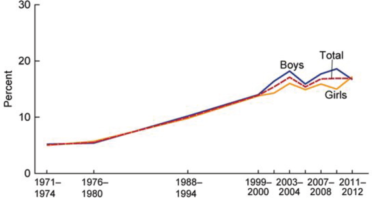
NOTE: Obesity was defined as a BMI greater than or equal to the sex- and age-specific 95th percentile from the 2000 Centers for Disease Control and Prevention Growth Chart.
SOURCE: Fryar et al., 2014.
and as such no nationally representative data were collected for these years. Similarly, NHANES did not resume data collection after 1994 until 1999. Accordingly, the time period between 1980 and 1988 and between 1994 and 1999 represent two spans of time in which the trend between time points were presumed to be linear. The data points from 1999 and later offer insight into how the estimates based on uniformly spaced cycles vary. It is clear that the change in obesity per year will vary significantly depending on the start and stop points on the curve (e.g. the slope is relatively flat from 1971-1980, with sharper increases 1999-2004). A rate of change calculated from 1971-2012 would be greater than that calculated from 2004-2012, highlighting the importance of the selection of start and stop points for characterizing trends.
The Presentation of Change
Published reports have used both absolute and relative change to describe how prevalence differs between two points in time. Absolute change is independent of the baseline prevalence, and is defined as the simple difference between the two estimates of prevalence (i.e., Prevalence2 – Prevalence1). Relative change, in contrast, is dependent on the initial value and is expressed as a percentage relative to the first point in time [i.e., (Prevalence2 – Prevalence1) / Prevalence1 × 100]. Not all published reports present both absolute and relative change. An understanding of which type of changes is being presented is fundamental for proper interpretation, as the two are not interchangeable. A report by Gee et al. (2013) serves as an illustrative example of how absolute and relative change describe the same data in different ways. The investigators estimated the prevalence of obesity among children ages 2 to 5 years who participated in an integrated health care delivery system to be 11.3 percent in 2003 and 10.0 percent in 2010. The investigators presented the absolute change as a 1.3 percentage point decrease (i.e., 10.0 – 11.3 = –1.3) and the relative change as 11.5 percent decrease [i.e., (10.0 – 11.3) / 11.3 × 100 = –11.5].
The difference between absolute and relative change also can be considered from the perspective of number of individuals affected. Figure 5-2 visualizes two hypothetical scenarios—one in which the initial prevalence is moderately elevated (50 percent; Scenario 1) and one in which the initial prevalence is particularly low (3 percent; Scenario 2). The absolute change of the two scenarios is equal (i.e., 2 percentage points), but the relative change is very different (i.e., 4 percent and 67 percent), highlighting the importance of the initial prevalence in interpreting the relative change. Additionally, the population size is an important consideration. When the population is of identical size across the two scenarios (i.e., 1,000/1,000), the same number of individuals would have changed weight status between
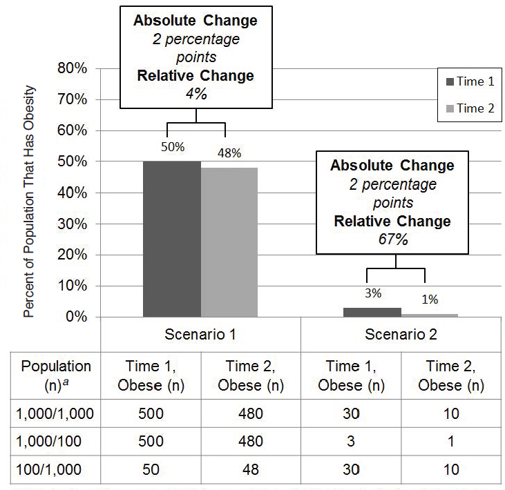
Time 1 and Time 2 (i.e., 20 individuals). Increases or decreases in the population—either across scenarios or across time points—can greatly alter the meaning. Sample size at both time points, therefore, is key information for interpreting estimates of change.
Changing Trends
Given the efforts dedicated to treating and preventing obesity, it is expected that the trend line will change slope and eventually change direction in the years ahead. From a statistical standpoint, the change in trend
can be assessed in different ways. Statistical hypothesis testing and construction of confidence intervals (CIs) are two closely related tools that are often used to assess whether trends are changing.3 Statistical hypothesis tests are used to evaluate a hypothesis (e.g., a null hypothesis of no change in obesity prevalence over a specified 10-year period), and test results are often summarized using a test statistic and p-value, with p-values <0.05 (indicating the almost ubiquitous 5 percent level of significance) most often deemed statistically significant and leading to rejection of the null hypothesis in favor of the alternative that obesity may indeed be changing with time. CIs are often used to indicate the precision associated with an estimate, with wider intervals indicating greater variability in estimation. The 95 percent CI, which is closely aligned with a 5 percent significance level in hypothesis testing, is by far the most common type of CI used. For example, an estimated prevalence of 26 percent with a 95 percent CI of 25 to 27 percent would be more precise than a 95 percent CI of 20 to 32 percent.
Joinpoint regression analysis is another technique that has been used to assess whether trends are changing (Kann et al., 2014; Pan et al., 2012).4 The general concept of joinpoint regression is to test whether a meaningful (i.e., statistically significant) change has occurred in the slope of a trend line for obesity prevalence estimates beyond that that could occur by chance. This test is helpful in detecting whether a previously increasing trend has flattened or changed into a decreasing trend. Generally, joinpoint analysis requires a relatively large number of time points and so is more relevant for studies across many years rather than studies with data from only a small number of years.
Comparative Evaluations
Comparative evaluations have been used to identify groups at disproportionate risk of obesity. These groups may represent those in most need of intervention or population groups that may need different types of intervention. The committee identified three common types of comparison that exist: comparisons of population groups within a report, comparisons across reports, and comparisons to NHANES. Consistent with its task, the committee also provides guidance for comparing obesity trends among diverse populations, both within and between reports (see Box 5-7).
___________________
3 For additional information on these concepts, see “Principles of Biostatistics” (Pagano and Gavreau, 2000).
4 For additional information on joinpoint, see Kim et al. (2000) and NCI (2016).
Comparing Population Groups Within a Report
When comparing subgroups of subjects in the same study, it is important to consider the subsample size and whether the same measurements and data collection techniques were applied in all subgroups. The precision of estimates is based on the sample size. When the sample size prevents a precise estimate, valid comparisons cannot be made. Another important consideration is that of misclassification of subjects in some subgroups but not in others, although, without having access to the raw data, it is difficult to ascertain the extent of misclassification within a given published report.
Comparing Across Reports
Several considerations impede comparisons between the results of one study to those of another. Design, sampling, and measurement issues are at the forefront of these considerations. Ideally, the studies should have been performed during the same time period in order to avoid the problem of secular changes that may apply to one but not both populations. The design and the inclusion and exclusion criteria should be the same in both studies in order to permit valid comparisons between studies. Similarly, the age, sex, racial, and ethnic composition of two populations should be the same to allow meaningful comparisons. Regional and geographic differences can also compromise comparisons between populations to the extent that such differences are present. Additionally, measurement issues emerge when comparing two populations. As discussed in Chapter 3, the comparability of directly measured and self- or proxy-reported heights and weights is limited. If different measurement tools are used without providing the necessary calibrations and conversion factors, then the study results cannot be meaningfully compared.
Comparing Reports to NHANES
Published reports have used NHANES estimates as a comparator for statistics derived from a different dataset. Shustak et al. (2012), for example, compared the prevalence of obesity among patients with and without congenital and acquired heart disease to obesity prevalence from NHANES data. Both datasets based BMI on directly measured height and weight and defined obesity as having a BMI at or above the 95th percentile on the 2000 CDC sex-specific BMI-for-age growth charts. Shustak et al. aligned the population groupings with NHANES in sex and age categories (2 to 5, 6 to 11, and 12 to 19 years). Data were collected over a similar time period (2005-2006 for NHANES versus 2006 heart disease sample). Another published report compared obesity prevalence in a sample of Special Olympics
participants to NHANES obesity prevalence estimates (Foley et al., 2014). In this report, the investigators used directly measured heights and weights, defined obesity as having a BMI at or above the 95th percentile according to the 2000 CDC BMI-for-age growth charts, and aligned data collection years. However, because participants cannot be enrolled in Special Olympics until age 8 years, age categories were 8 to 11 years and 12 to 17 years, whereas the NHANES analysis categorized ages as 6 to 11 and 12 to 17 years. These examples illustrate that alignment of available demographic characteristics, data collection methodologies, and years included serve as the foundation for considering such comparisons.
Similarities of study results with NHANES results should not be used as an indicator of the validity of those results, as NHANES results represent the average estimate (or central tendency measure) for the entire U.S. population, and have been known to mask levels or trends that vary in some regions or parts of the country or among demographic groups that may not be represented adequately in national samples.
SUMMARY
Estimates of obesity prevalence and trends reside in published reports with a variety of purposes. The published report’s purpose can provide insight into why a data source was selected and why specific analytic decisions were made. A range of analytic decisions affect the interpretation of the resulting statistic of obesity prevalence, change, or trend, and occur both in the preparation of the data and the statistical analysis of the data.
In preparing the data, investigators must classify obesity status, and can elect to identify BIVs and evaluate the representativeness of the data source, as appropriate. For children, adolescents, and young adults, the 2000 CDC BMI-for-age growth charts are most typically used, but others exist, such as the IOTF cut points and the WHO growth charts. Use of different reference populations can lead to different estimates of obesity prevalence. A range of different methods exists for identifying and handling BIVs across published reports, which can affect estimates of obesity prevalence. Potential sources of bias related to the population in a dataset can be assessed through the study design, response rates, and amount of data that are missing. Weighting a sample is one approach to correct for imperfections in sampling, account for non-response, and better represent the target population described by the estimates, although not all datasets will need to be weighted.
The statistical analysis that produces an estimate of obesity prevalence or trend is guided by the analytic sample size and the interpretation of the estimate informed by the population groups and the time points it encompasses. The analytic sample size determines what statistical procedures and comparisons can be meaningfully conducted. Prevalence estimates that
encompass diverse population groups may not adequately describe the variability that exists within the subgroups it contains. The time frame used in trends analyses is crucial to interpreting the findings. Analyses using the same data source but different time frames can reach different conclusions. Ample sample size, similar data collection methodologies, and adequate characterization of population groups facilitate the ability to compare obesity prevalence and trends estimates across subgroups and between reports.
REFERENCES
AAPOR (American Association for Public Opinion Research). 2008. Standard definitions: Final dispositions of case codes and outcome rates for surveys. 5th ed. Lenexa, KS: AAPOR.
AAPOR. 2016. Response rates—an overview. http://www.aapor.org/Education-Resources/ForResearchers/Poll-Survey-FAQ/Response-Rates-An-Overview.aspx (accessed March 25, 2016).
AHRQ (Agency for Healthcare Research and Quality). 2009. 1996-2007 pooled estimation file. http://meps.ahrq.gov/mepsweb/data_stats/download_data/pufs/h36/h36u07doc.shtml (accessed March 25, 2016).
Aryana, M., Z. Li, and W. J. Bommer. 2012. Obesity and physical fitness in California school children. American Heart Journal 163(2):302-312.
Benson, L., H. J. Baer, and D. C. Kaelber. 2009. Trends in the diagnosis of overweight and obesity in children and adolescents: 1999-2007. Pediatrics 123(1):e153-e158.
Benson, L. J., H. J. Baer, and D. C. Kaelber. 2011. Screening for obesity-related complications among obese children and adolescents: 1999-2008. Obesity (Silver Spring) 19(5):1077-1082.
California Department of Education. 2013. Dataquest. http://data1.cde.ca.gov/dataquest (accessed March 14, 2016).
California Department of Education. 2016. FitnessGram: Healthy fitness zone charts. http://www.cde.ca.gov/ta/tg/pf/healthfitzones.asp (accessed March 25, 2016).
CDC (Centers for Disease Control and Prevention). 2002. 2000 CDC growth charts for the United States: Methods and development. Vital and Health Statistics 11 (246).
CDC. 2010. Growth charts. http://www.cdc.gov/growthcharts/index.htm (accessed February 17, 2016).
CDC. 2013a. Continuous NHANES web tutorial: Sample design. http://www.cdc.gov/nchs/tutorials/NHANES/SurveyDesign/SampleDesign/intro.htm (accessed March 25, 2016).
CDC. 2013b. Methodology of the Youth Risk Behavior Surveillance System—2013. Morbidity and Mortality Weekly Report 62(1).
CDC. 2013c. National Health and Nutrition Examination Survey (NHANES) anthropometry procedures manual. http://www.cdc.gov/nchs/data/nhanes/nhanes_13_14/2013_Anthropometry.pdf (accessed June 7, 2016).
CDC. 2013d. National Health and Nutrition Examination Survey: Analytic guidelines, 1999-2010. Vital and Health Statistics 2(161).
CDC. 2013e. Obesity in K-7 students—Anchorage, Alaska, 2003-04 to 2010-11 school years. Morbidity and Mortality Weekly Report 62(21):426-430.
CDC. 2014. 2013 YRBS data user’s guide. http://www.cdc.gov/healthyyouth/yrbs/pdf/YRBS_2013_National_User_Guide.pdf (accessed March 11, 2016).
CDC. 2015a. BMI Percentile Calculator for Child and Teen. http://nccd.cdc.gov/dnpabmi/Calculator.aspx (accessed March 10, 2016).
CDC. 2015b. Childhood obesity facts. http://www.cdc.gov/healthyschools/obesity/facts.htm (accessed March 25, 2016).
CDC. 2015c. Children’s BMI tool for schools. http://www.cdc.gov/healthyweight/assessing/bmi/childrens_BMI/tool_for_schools.html (accessed March 10, 2016).
CDC. 2015d. A SAS program for the 2000 CDC growth charts (ages 0 to <20 years). http://www.cdc.gov/nccdphp/dnpao/growthcharts/resources/sas.htm (accessed September 29, 2015).
CDC. 2016a. The CDC growth chart reference population. http://www.cdc.gov/nccdphp/dnpao/growthcharts/training/overview/page4.html (accessed March 10, 2016).
CDC. 2016b. Cut-offs to define outliers in the 2000 CDC growth charts. http://www.cdc.gov/nccdphp/dnpao/growthcharts/resources/biv-cutoffs.pdf (accessed March 10, 2016).
Cole, T. J., and T. Lobstein. 2012. Extended international (IOTF) body mass index cut-offs for thinness, overweight and obesity. Pediatric Obesity 7(4):284-294.
Cole, T. J., M. C. Bellizzi, K. M. Flegal, and W. H. Dietz. 2000. Establishing a standard definition for child overweight and obesity worldwide: International survey. BMJ 320(7244):1240-1243.
Day, S. E., K. J. Konty, M. Leventer-Roberts, C. Nonas, and T. G. Harris. 2014. Severe obesity among children in New York City public elementary and middle schools, school years 2006-07 through 2010-11. Preventing Chronic Disease 11:E118.
de Onis, M., C. Garza, C. G. Victoria, A. W. Onyango, E. A. Frongillo, and J. Martines. 2004. The WHO Multicentre Growth Reference Study: Planning, study design, and methodology. Food and Nutrition Bulletin 25(Suppl 1):S15-S26.
de Onis, M., A. W. Onyango, E. Borghi, A. Siyam, C. Nishida, and J. Siekmann. 2007. Development of a WHO growth reference for school-aged children and adolescents. Bulletin of the Wold Health Organization 85(9):660-667.
Ezendam, N. P., A. E. Springer, J. Brug, A. Oenema, and D. H. Hoelscher. 2011. Do trends in physical activity, sedentary, and dietary behaviors support trends in obesity prevalence in 2 border regions in Texas? Journal of Nutrition Education and Behavior 43(4):210-218.
Flegal, K. M., and T. J. Cole. 2013. Construction of LMS parameters for the Centers for Disease Control and Prevention 2000 growth charts. National Health Statistics Reports (63):1-3.
Flegal, K. M., and C. L. Ogden. 2011. Childhood obesity: Are we all speaking the same language? Advances in Nutrition: An International Review Journal 2(2):159S-166S.
Flegal, K. M., R. Wei, C. L. Ogden, D. S. Freedman, C. L. Johnson, and L. R. Curtin. 2009. Characterizing extreme values of body mass index-for-age by using the 2000 Centers for Disease Control and Prevention growth charts. American Journal of Clinical Nutrition 90(5):1314-1320.
Foley, J. T., M. Lloyd, D. Vogl, and V. A. Temple. 2014. Obesity trends of 8-18 year old Special Olympians: 2005-2010. Research in Developmental Disabilities 35(3):705-710.
Freedman, D. S., L. K. Khan, M. K. Serdula, C. L. Ogden, and W. H. Dietz. 2006. Racial and ethnic differences in secular trends for childhood BMI, weight, and height. Obesity (Silver Spring) 14(2):301-308.
Freedman, D. S., C. L. Ogden, and S. E. Cusick. 2011. The measurement and epidemiology of child obesity. In Global perspectives on childhood obesity, edited by D. Bagchi. Burlington, MA: Elsevier.
Freedman, D. S., A. Goodman, O. A. Contreras, P. DasMahapatra, S. R. Srinivasan, and G. S. Berenson. 2012. Secular trends in BMI and blood pressure among children and adolescents: The Bogalusa Heart Study. Pediatrics 130(1):e159-e166.
Freedman, D. S., H. G. Lawman, A. C. Skinner, L. C. McGuire, D. B. Allison, and C. L. Ogden. 2015. Validity of the WHO cutoffs for biologically implausible values of weight, height, and BMI in children and adolescents in NHANES from 1999 through 2012. American Journal of Clinical Nutrition 102(5):1000-1006.
Fryar, C. D., M. D. Carroll, and C. L. Ogden. 2014. Prevalence of overweight and obesity among children and adolescents: United States, 1963-1965 through 2011-2012. http://www.cdc.gov/nchs/data/hestat/obesity_child_11_12/obesity_child_11_12.pdf (accessed February 17, 2016).
Gadbury, G. L., C. S. Coffey, and D. B. Allison. 2003. Modern statistical methods for handling missing repeated measurements in obesity trial data: Beyond LOCF. Obesity Reviews 4(3):175-184.
Garza, C., and M. de Onis. 2004. Rationale for developing a new international growth reference. Food and Nutrition Bulletin 25 (Supplement 1):S5-S14.
Gee, S., D. Chin, L. Ackerson, D. Woo, and A. Howell. 2013. Prevalence of childhood and adolescent overweight and obesity from 2003 to 2010 in an integrated health care delivery system. Journal of Obesity 2013:417907.
Grummer-Strawn, L. M., C. Reinold, and N. F. Krebs. 2010. Use of World Health Organization and CDC growth charts for children aged 0-59 months in the United States. MMWR Recommendations and Reports 59(Rr-9):1-15.
Hinkle, S. N., A. J. Sharma, S. Y. Kim, S. Park, K. Dalenius, P. L. Brindley, and L. M. Grummer-Strawn. 2012. Prepregnancy obesity trends among low-income women, United States, 1999-2008. Maternal and Child Health Journal 16(7):1339-1348.
Iannotti, R. J., and J. Wang. 2013. Trends in physical activity, sedentary behavior, diet, and BMI among US adolescents, 2001-2009. Pediatrics 132(4):606-614.
JAMA (Journal of the American Medical Association). 2016. JAMA instructions for authors. http://jama.jamanetwork.com/public/instructionsForAuthors.aspx (accessed May 12, 2016).
Jin, Y., and J. C. Jones-Smith. 2015. Associations between family income and children’s physical fitness and obesity in California, 2010-2012. Preventing Chronic Disease 12:E17.
Johnson, C. L., R. Paulose-Ram, and C. L. Ogden. 2013. National Health and Nutrition Examination Survey: Analytic guidelines, 1999-2010. Vital and Health Statistics 2 (161).
Kann, L., S. Kinchen, S. L. Shanklin, K. H. Flint, J. Kawkins, W. A. Harris, R. Lowry, E. O. Olsen, T. McManus, D. Chyen, L. Whittle, E. Taylor, Z. Demissie, N. Brener, J. Thornton, J. Moore, and S. Zaza. 2014. Youth Risk Behavior Surveillance—United States, 2013. MMWR Surveillance Summaries 63(Suppl 4):1-168.
Keeter, S., C. Kennedy, D. Michael, J. Best, and C. Peyton. 2006. Gauging the impact of growing nonresponse on estimates from a national RDD telephone survey. The Public Opinion Quarterly 70(5):759-779.
Kim, H. J., M. P. Fay, E. J. Feuer, and D. N. Midthune. 2000. Permutation tests for joinpoint regression with applications to cancer rates. Statistics in Medicine 19(3):335-351.
Kim, J., B. Mutyala, S. Agiovlasitis, and B. Fernhall. 2011. Health behaviors and obesity among US children with attention deficit hyperactivity disorder by gender and medication use. Preventive Medicine 52(3-4):218-222.
Kish, L. 1965. Survey sampling. New York: John Wiley & Sons, Inc.
Kuczmarski, R. J., C. L. Ogden, L. M. Grummer-Strawn, K. M. Flegal, S. S. Guo, R. Wei, Z. Mei, L. R. Curtin, A. F. Roche, and C. L. Johnson. 2000. CDC growth charts: United States. Advance Data 314.
Lang, I. A., R. R. Kipping, R. Jago, and D. A. Lawlor. 2011. Variation in childhood and adolescent obesity prevalence defined by international and country-specific criteria in England and the United States. European Journal of Clinical Nutrition 65(2):143-150.
Lawman, H. G., C. L. Ogden, S. Hassink, G. Mallya, S. Vander Veur, and G. D. Foster. 2015. Comparing methods for identifying biologically implausible values in height, weight, and body mass index among youth. American Journal of Epidemiology 182(4):359-365.
The Lewin Group. 1998. Deriving state-level estimates from three national surveys: A statistical assessment and state tabulations. Falls Church, VA: The Lewin Group.
Li, W., J. H. Buszkiewicz, R. B. Leibowitz, M. A. Gapinski, L. J. Nasuti, and T. G. Land. 2015. Declining trends and widening disparities in overweight and obesity prevalence among Massachusetts public school districts, 2009-2014. American Journal of Public Health 105(10):e76-e82.
Little, R. J., R. D’Agostino, M. L. Cohen, K. Dickersin, S. S. Emerson, J. T. Farrar, C. Frangakis, J. W. Hogan, G. Molenberghs, S. A. Murphy, J. D. Neaton, A. Rotnitzky, D. Scharfstein, W. J. Shih, J. P. Siegel, and H. Stern. 2012. The prevention and treatment of missing data in clinical trials. New England Journal of Medicine 367(14):1355-1360.
Maalouf-Manasseh, Z., E. Metallinos-Katsaras, and K. G. Dewey. 2011. Obesity in preschool children is more prevalent and identified at a younger age when WHO growth charts are used compared with CDC charts. Journal of Nutrition 141(6):1154-1158.
Madsen, K. A., A. E. Weedn, and P. B. Crawford. 2010. Disparities in peaks, plateaus, and declines in prevalence of high BMI among adolescents. Pediatrics 126(3):434-442.
Mei, Z., C. L. Ogden, K. M. Flegal, and L. M. Grummer-Strawn. 2008. Comparison of the prevalence of shortness, underweight, and overweight among US children aged 0 to 59 months by using the CDC 2000 and the WHO 2006 growth charts. Journal of Pediatrics 153(5):622-628.
NCHS (National Center for Health Statistics). 2012. Task 2: When and how to construct weights when combining survey cycles. http://www.cdc.gov/nchs/tutorials/NHANES/SurveyDesign/Weighting/Task2.htm (accessed March 25, 2016).
NCI (National Cancer Institute). 2016. Joinpoint trend analysis software. http://surveillance.cancer.gov/joinpoint (accessed May 12, 2016).
NRC (National Research Council). 2010. The prevention and treatment of missing data in clinical trials. Washington, DC: The National Academies Press.
NYC (New York City) Department of Education. 2016. NYC FitnessGram: For families. http://schools.nyc.gov/Academics/FitnessandHealth/NycFitnessgram/families/default.htm (accessed March 25, 2016).
Ogden, C. L. 2015. Obesity in the US: Beyond the data. PowerPoint presentation at Evaluating Approaches to Assessing Prevalence and Trends In Obesity: Data Gathering Public Workshop, Washington, DC.
Ogden, C. L., M. D. Carroll, B. K. Kit, and K. M. Flegal. 2012. Prevalence of obesity and trends in body mass index among US children and adolescents, 1999-2010. Journal of the American Medical Association 307(5):483-490.
Ogden, C. L., M. D. Carroll, B. K. Kit, and K. M. Flegal. 2014. Prevalence of childhood and adult obesity in the United States, 2011-2012. Journal of the American Medical Association 311(8):806-814.
Osborne, J. W. 2011. Best practices in using large, complex samples: The importance of using appropriate weights and design effect compensation. Practical Assessment, Research, and Evaluation 16(12):1-7.
Pagano, M., and K. Gavreau. 2000. Principles of biostatistics. 2nd ed. Duxbury, MA: Duxbury Press.
Pan, L., H. M. Blanck, B. Sherry, K. Dalenius, and L. M. Grummer-Strawn. 2012. Trends in the prevalence of extreme obesity among US preschool-aged children living in low-income families, 1998-2010. Journal of the American Medical Association 308(24):2563-2565.
Robbins, J. M., G. Mallya, A. Wagner, and J. W. Buehler. 2015. Prevalence, disparities, and trends in obesity and severe obesity among students in the school district of Philadelphia, Pennsylvania, 2006-2013. Preventing Chronic Disease 12:E134.
Robinson, W. R., K. M. Keyes, R. L. Utz, C. L. Martin, and Y. Yang. 2013. Birth cohort effects among US-born adults born in the 1980s: Foreshadowing future trends in US obesity prevalence. International Journal of Obesity (London) 37(3):448-454.
Rodriguez-Colon, S. M., E. O. Bixler, X. Li, A. N. Vgontzas, and D. Liao. 2011. Obesity is associated with impaired cardiac autonomic modulation in children. International Journal of Pediatric Obesity 6(2):128-134.
Saab, P. G., S. Fitzpatrick, B. Lai, and J. R. McCalla. 2011. Elevated body mass index and obesity among ethnically diverse adolescents. Ethnicity & Disease 21.
Sanchez, B. N., E. V. Sanchez-Vaznaugh, A. Uscilka, J. Baek, and L. Zhang. 2012. Differential associations between the food environment near schools and childhood overweight across race/ethnicity, gender, and grade. American Journal of Epidemiology 175(12):1284-1293.
Schafer, J. L., and J. W. Graham. 2002. Missing data: Our view of the state of the art. Psychological Methods 7(2):147-177.
Sekhobo, J. P., L. S. Edmunds, D. K. Reynolds, K. Dalenius, and A. Sharma. 2010. Trends in prevalence of obesity and overweight among children enrolled in the New York State WIC program, 2002-2007. Public Health Reports 125(2):218-224.
Sekhobo, J. P., L. S. Edmunds, K. Dalenius, J. Jernigan, C. F. Davis, M. Giddings, C. Lesesne, and L. Kettel Khan. 2014. Neighborhood disparities in prevalence of childhood obesity among low-income children before and after implementation of New York City child care regulations. Preventing Chronic Disease 11:E181.
Shustak, R. J., S. B. McGuire, T. W. October, C. K. Phoon, and A. J. Chun. 2012. Prevalence of obesity among patients with congenital and acquired heart disease. Pediatric Cardiology 33(1):8-14.
Skinner, A. C., and J. A. Skelton. 2014. Prevalence and trends in obesity and severe obesity among children in the United States, 1999-2012. JAMA Pediatrics 168(6):561-566.
Ver Ploeg, M., L. Mancino, B. H. Lin, and J. Guthrie. 2008. US food assistance programs and trends in children’s weight. Internaitonal Journal of Pediatric Obesity 3(1):22-30.
Villar, J., A. T. Papageorghiou, and R. Pang, et al. 2014. The likeness of fetal growth and newborn size across non-isolated populations in the INTERGROWTH-21st project: The fetal growth longitudinal study and newborn cross-sectional study. Lancet Diabetes and Endocrinology 2(10):781-792.
von Hippel, P. T., and R. W. Nahhas. 2013. Extending the history of child obesity in the United States: The Fels Longitudinal Study, birth years 1930-1993. Obesity (Silver Spring) 21(10):2153-2156.
Wang, Y., and H.-J. Chen. 2012. Use of percentiles and z-scores in anthropometry. In Handbook of anthropometry. Vol. 1, edited by V. R. Preedy. New York: Springer.
Weedn, A. E., J. J. Hale, D. M. Thompson, and P. M. Darden. 2014. Trends in obesity prevalence and disparities among low-income children in Oklahoma, 2005-2010. Child Obesity 10(4):318-325.
WHO (World Health Organization). 1995. Physical status: The use and interpretation of anthropometry. Geneva: World Health Organization.
WHO MGRS (World Health Organization Multicentre Growth Reference Study). 2006. Assessment of differences in linear growth among populations in the WHO Multicentre Growth Reference Study. Acta Paediatrica Suppement 450:56-65.
Williamson, D. A., H. Han, W. D. Johnson, T. M. Stewart, and D. W. Harsha. 2011. Longitudinal study of body weight changes in children: Who is gaining and who is losing weight. Obesity (Silver Spring) 19(3):667-670.
YRBSS (Youth Risk Behavior Surveillance Survey). 2014. Combining YRBS data across years and sites. Centers for Disease Control and Prevention.
Zhang, X., S. Onufrak, J. B. Holt, and J. B. Croft. 2013. A multilevel approach to estimating small area childhood obesity prevalence at the census block-group level. Preventing Chronic Disease 10:E68.
This page intentionally left blank.


