Guidance for Design Hydrology for Stream Restoration and Channel Stability (2017)

Below is the uncorrected machine-read text of this chapter, intended to provide our own search engines and external engines with highly rich, chapter-representative searchable text of each book. Because it is UNCORRECTED material, please consider the following text as a useful but insufficient proxy for the authoritative book pages.

14 C h a p t e r 3 3.1 Guidance/Examples Overview The following subsections provide some guidance and step-by-step examples for several of the tools: • Subsection 3.2: Guidance for Calculating the Half-Load Discharge (Qs50) • Subsection 3.3: Examples – Subsection 3.3.1: Example 1: Projecting hydrologic changes caused by changing land use for the Fourmile Creek watershed in central Iowa (Step 1) – Subsection 3.3.2: Example 2: Rainfall-Runoff Modeling of Box Elder Creek (Step 3) – Subsection 3.3.3: Example 3: Using eRAMS to calculate the Richards-Baker Flashiness Index of the Iowa River near Iowa City, Iowa (Step 5) – Subsection 3.3.4: Example 4: Using the Qs50 decision tree for determining Qs50 for the Iowa River near Iowa City, Iowa (Steps 1 Through 5) Chapter 4 provides step-by-step guidance for each tab in the CSR Tool workbook. Chapter 5 presents two examples (sand bed and gravel/cobble bed) using the CSR Tool. 3.2 Guidance for Calculating the Half-Load Discharge 3.2.1 Step 1: Projecting Future Streamflow Behavior Caused by Changing Land Use If a substantial change in land use in the basin is expected over the time period of interest, historical streamflow records may not act as a good predictor of future streamflow behavior. Hydrological models can be used to assess how much the flow regime is likely to change with changes in land use, and, if significant changes are likely to occur, models may be used to generate streamflow data consistent with future land use. Many hydrological models have been applied to evaluate potential hydrologic impacts of basin- scale climate change and urban development (Praskievicz and Chang 2009), and some state agencies employ their own models for continuous hydrologic simulation (e.g., the Western Washington Continuous Simulation Hydrology Model 2012). Regardless of the chosen hydrological model, the hydrologic importance of potential future land use change may be evaluated by comparing model-predicted FDCs for current and projected land use scenarios. If a shift in the FDC due to land use change is predicted, it may be more appropriate to use the model-predicted FDC than historical streamflow records. Although uncalibrated models may accurately predict the direction of change in streamflow associated with land use change, accurate prediction of the magnitude of those changes likely requires a spatially calibrated model (Niraula et al. 2015). See Example 1 for an illustration of how the SWAT-DEG tool in eRAMS may be used to assess shifts in an FDC due to potential land use changes. Guidance/Examples

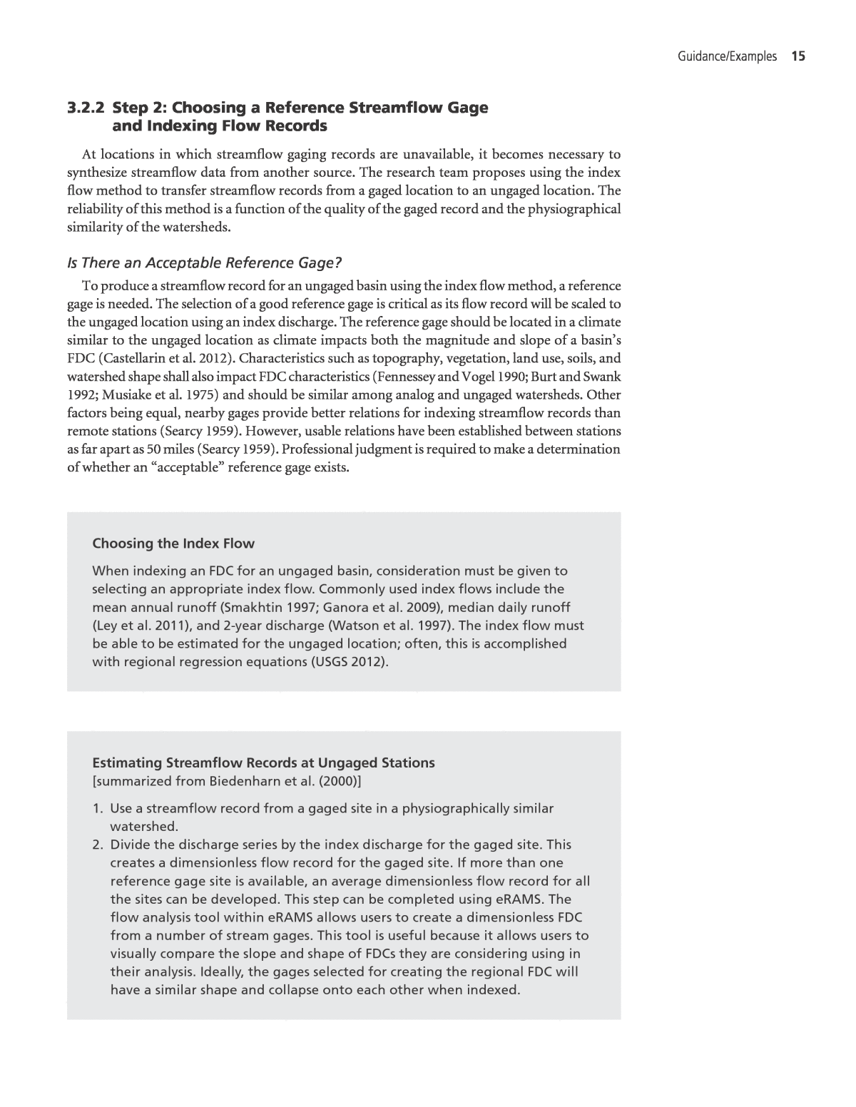
Guidance/examples 15 3.2.2 Step 2: Choosing a Reference Streamflow Gage and Indexing Flow Records At locations in which streamflow gaging records are unavailable, it becomes necessary to synthesize streamflow data from another source. The research team proposes using the index flow method to transfer streamflow records from a gaged location to an ungaged location. The reliability of this method is a function of the quality of the gaged record and the physiographical similarity of the watersheds. Is There an Acceptable Reference Gage? To produce a streamflow record for an ungaged basin using the index flow method, a reference gage is needed. The selection of a good reference gage is critical as its flow record will be scaled to the ungaged location using an index discharge. The reference gage should be located in a climate similar to the ungaged location as climate impacts both the magnitude and slope of a basin’s FDC (Castellarin et al. 2012). Characteristics such as topography, vegetation, land use, soils, and watershed shape shall also impact FDC characteristics (Fennessey and Vogel 1990; Burt and Swank 1992; Musiake et al. 1975) and should be similar among analog and ungaged watersheds. Other factors being equal, nearby gages provide better relations for indexing streamflow records than remote stations (Searcy 1959). However, usable relations have been established between stations as far apart as 50 miles (Searcy 1959). Professional judgment is required to make a determination of whether an “acceptable” reference gage exists. Choosing the Index Flow When indexing an FDC for an ungaged basin, consideration must be given to selecting an appropriate index flow. Commonly used index flows include the mean annual runoff (Smakhtin 1997; Ganora et al. 2009), median daily runoff (Ley et al. 2011), and 2-year discharge (Watson et al. 1997). The index flow must be able to be estimated for the ungaged location; often, this is accomplished with regional regression equations (USGS 2012). Estimating Streamflow Records at Ungaged Stations [summarized from Biedenharn et al. (2000)] 1. Use a streamflow record from a gaged site in a physiographically similar watershed. 2. Divide the discharge series by the index discharge for the gaged site. This creates a dimensionless flow record for the gaged site. If more than one reference gage site is available, an average dimensionless flow record for all the sites can be developed. This step can be completed using eRAMS. The flow analysis tool within eRAMS allows users to create a dimensionless FDC from a number of stream gages. This tool is useful because it allows users to visually compare the slope and shape of FDCs they are considering using in their analysis. Ideally, the gages selected for creating the regional FDC will have a similar shape and collapse onto each other when indexed.

16 Guidelines for Design hydrology for Stream restoration and Channel Stability 3.2.3 Step 3: Using a Hydrologic Model to Produce Streamflow Time Series from Precipitation Records Many methods and software packages exist for rainfall-runoff modeling, for an introduc- tion, see Beven (2011). The SWAT-DEG Tool within eRAMS is a great resource for developing streamflow records from climatic data for watersheds throughout the country. An example of this application is given in Subsection 3.3.2 for Box Elder Creek in northern Colorado. 3.2.4 Step 4: Checking the Stationarity of Streamflow Records Because some regions may be experiencing changes in climate that render historical hydro- logic records less effective (Milly 2007), it is critical that the stationarity of a hydrologic record be checked before it is used. Methods for testing the stationarity of historical hydrologic records include Mann-Kendall testing (Hamed 2008; Kumar et al. 2009), Spearman’s rank correlation method (Villarini et al. 2009; Kahya and Kalayci 2004), and Sen’s slope (Kahya and Kalayci 2004). If the streamflow record is highly non-stationary, a hydrologic model may be appropri- ate for developing streamflow records. For gaged sites, a flow record of at least 15 to 20 years is needed to detect non-stationary behavior, especially for watersheds with inherently high values of R-B Index (see next subsection) and coefficient of variation. 3.2.5 Step 5: Calculating the Richards-Baker Flashiness Index The R-B Index is calculated by first calculating the path length of flow changes over a given period of time. The path length is equal to the sum of the absolute values of day-to-day changes in discharge. This path length is then divided by the sum of mean daily flows. The R-B Index is high for flashy hydrographs and low when hydrographs rise and fall gradually. The R-B Index is shown in Equation 3-1: R-B Index (3-1) 11 1 q q q i ii n ii n ∑ ∑= − − = = where: q = daily-averaged discharge [m2/s]; i = day; and n = total number of days in the flow record. 3.2.6 Step 6: Obtaining a Sediment Rating Curve Gaged Sites If sediment transport measurements exist at a given site for a range of discharges, a sediment rating curve can be constructed. Sediment rating curves often take the form of a simple power See Example 2 for an example application of rainfall-runoff modeling using the SWAT-DEG tool in eRAMS. The R-B Index can be calcu- lated at gaged sites using the eRAMS Flow Analysis Tool. This is illustrated in Example 3. 3. Compute the index flow for the ungaged site using regional regression equa- tions (available from the National Streamflow Statistics Program: http://water. usgs.gov/osw/programs/nss/index.html). 4. Calculate the streamflow record for the ungaged site by multiplying the dimensionless flow record by the index discharge for the ungaged site.

Guidance/examples 17 In instances where channel geometry measurements are not available, and collecting sediment transport data is cost or time prohibitive, other methods exist for estimating sediment rating curve parameters. The eRAMS platform has the functionality to provide sediment transport capacity estimates at vary- ing discharges for either extracted or imported cross sections. To make these estimates, eRAMS allows the user to use either the Brownlie (1981), Bagnold (1980), or Wilcock-Kenworthy (2002) equations. The eRAMS platform will also perform the necessary regression and provide the user with the resultant sediment rating curve parameters. These capabilities are located within the channel cross-section analysis application (currently available at https://beta. erams.com/). function: Qs = aQb; where Qs = sediment discharge rate, Q = water discharge rate [m3/s], and a, b = best-fit regression parameters (Asselman 2000). Ungaged Sites For sites in which sediment transport measurements are not available, a range of options exist for synthesizing a sediment rating curve. If the channel geometry and slope measurements are available at the site, bedload or total load sediment transport equations can be used to create a sediment rating curve as appropriate based on the bed material and hydraulic conditions. Such equations provide an estimate of sediment transport rate for a given discharge and, by estimat- ing the sediment transport at a range of discharges, a sediment rating curve can be established. It is very important to use an equation that is calibrated and tested for the conditions to which it is applied. Sediment rating curves can also be estimated using generalized regression equations for ungaged sites (e.g., Syvitski et al. 2000). While rating curve coefficients and exponents may be predicted based on factors such as basin relief, mean annual air temperature, and latitude, such an approach is susceptible to large errors and may not reflect important local sources of sedi- ment in a particular watershed context. 3.2.7 Step 7: Determining the Appropriate Resolution of Streamflow Data Streamflow gaging stations in the United States generally provide data in both daily-averaged and 15-minute increments. Daily-averaged discharges, while convenient to use, may not always be appropriate for sediment transport calculations. Streams in urban areas or arid climates, or with small drainage areas, may exhibit rapid short-term variations in streamflow (Ågren et al. 2007; Graf 1977; Walsh et al. 2005). This type of streamflow is often termed “flashy.” Flashy streams may have flood events lasting only a few hours, causing the peak discharge to be much greater than the corresponding mean daily discharge (Biedenharn et al. 2000). In these situa- tions, sediment transport can be underestimated. The degree of underestimation is a function of stream flashiness and the logarithmic slope of the sediment rating curve, b (Rosburg 2015). Using Figure 3-1, one can estimate the underestimation in Qs50 that would result from using daily-averaged flow data, instead of hourly flow data, as a function of the R-B Index (Baker et al. 2004) and sediment rating curve parameter, b.

18 Guidelines for Design hydrology for Stream restoration and Channel Stability 3.3 Examples Much of the analysis needed to determine Qs50 for a given site can be facilitated using tools built into eRAMS. These capabilities are illustrated in the following four examples. 3.3.1 Example 1: Projecting Hydrologic Changes Caused by Changing Land Use for the Fourmile Creek Watershed in Central Iowa (Step 1) The Fourmile Creek watershed is a 300 km2 basin located north and east of Des Moines, Iowa (Figure 3-2). This example explores the hydrologic sensitivity of Fourmile Creek to urbaniza- tion using the eRAMS SWAT-DEG Tool. As of the year 2010, 36% of the watershed was classi- fied as urban, and it is expected that the proportion of urban area will increase. Therefore, two hypothetical scenarios were developed to explore how increases in urban area would impact hydrologic conditions. In Scenario 1, urban area was increased to 50% of watershed area and cropland decreased to 38%. In Scenario 2, urban area was increased to 75% of watershed area and cropland was decreased to 13% (Table 3-1). Running SWAT-DEG within eRAMS requires, at a minimum, watershed information, chan- nel information, and climate data for the time period of interest. Once a new project has been created, the user can populate the watershed properties by extracting data from a user-defined watershed, or can simply enter the data directly if they are known. To facilitate the use of cli- mate data, eRAMS allows users to download daily climate observations from the Global Histori- cal Climatology Network—Daily (GHCND). The eRAMS interface where the data are input is shown in Figure 3-3. Following the data input, the user can click “Run SWAT-DEG” to run the model and view the results. The “Results” tab displays the various scenarios the user created and allows the user Figure 3-1. Percentage of underestimation of the half-load discharge (Qs50) (values labeled at the top of contours) when it is calculated with daily-averaged flow data instead of hourly flow data for (a) bedload sites and (b) suspended-load sites.

Guidance/examples 19 to choose and graph outputs. Outputs can also be downloaded in a variety of formats for post- processing. The research team’s investigation into the hydrologic impacts of urbanization for Fourmile Creek suggests that increases in urbanization will likely cause increases in the magni- tude of the FDC across nearly all exceedance levels (Figure 3-4). This demonstrates that historic streamflow records may not be appropriate for future land use conditions. 3.3.2 Example 2: Rainfall-Runoff Modeling of Box Elder Creek (Step 3) Box Elder Creek is a 750 km2 watershed located in northern Colorado and southern Wyoming (Figure 3-5). Because the creek is ungaged, streamflow records are unavailable. Additionally, because the southern portion of the basin is undergoing rapid urbanization, indexing a flow Figure 3-2. Fourmile Creek watershed. Table 3-1. Current and future land use scenarios. Land Use Year 2010* Future Scenario 1 Future Scenario 2 Urban and Rural Residential 36% 50% 75% Forest 1% 1% 1% Crop Land 52% 38% 13% Pasture/Grassland 11% 11% 11% Other 0% 0% 0% * Adapted from Snyder & Associates Inc. (2013).

20 Guidelines for Design hydrology for Stream restoration and Channel Stability Figure 3-3. eRAMS SWAT-DEG interface. Figure 3-4. Comparison of current and future land use FDCs for Fourmile Creek. Created with data produced by eRAMS SWAT-DEG Tool. 1 10 100 1000 0 20 40 60 80 100 Fl ow (m 3 /s ) Time flow is exceeded (%) Fourmile Creek - Des Moines, IA 2010 Future Scenario 2 Future Scenario 1

Guidance/examples 21 record from a similar and nearby gage is not the best option. This leaves hydrologic modeling as the best remaining option for obtaining a streamflow series at this site. After logging into eRAMS and starting a new SWAT-DEG project, the user is required to input watershed properties, channel information, and climate data for the time period of interest. The user can populate the watershed properties by extracting data from a user-defined watershed or can simply enter the data directly if they are known. To obtain climate data, eRAMS allows users to download GHCND data. The required input information for Box Elder Creek is shown in Figure 3-6. After fully populating the input screen, the user can run the model by clicking “Run SWAT- DEG.” This runs the model and launches the output screen. Streamflow data can then be obtained by selecting the appropriate scenario and output parameter and clicking “Graph Out- put.” A plot of the streamflow time series will then be made available as shown in Figure 3-7. The start and end of the streamflow time series correspond to the start year and simulation length selected when the scenario was developed. It is important to note that the user is required to have climatology data for the entire simulation period. After the model runs, the raw streamflow data can be downloaded by clicking in the upper right-hand corner of the graph and choosing a preferred file format. Currently, streamflow data are only available in millimeters per day. This can be converted to cubic meters per second by multiplying by the drainage area (m2) and 86.4. Future versions of eRAMS will do this conver- sion automatically and provide streamflow in cubic meters per second. Figure 3-5. Box Elder Creek watershed.

Figure 3-6. eRAMS SWAT-DEG inputs for Box Elder Creek, Colorado. Figure 3-7. Daily series of streamflow for Box Elder Creek.

Guidance/examples 23 3.3.3 Example 3: Using eRAMS to Calculate the Richards-Baker Flashiness Index of the Iowa River near Iowa City, Iowa (Step 5) After signing into eRAMS.com and starting a new “Flow Analysis” project, the user can select a streamflow gage of interest. This can be accomplished by searching for a USGS station by name or keyword, or by drawing a rectangle or polygon on the map. Once the gage has been selected, the user clicks the “Flow Analysis Model” link to launch the application (Figure 3-8). The user then proceeds to the “Data” tab and specifies the preferred time series, analysis period, and parameter (Figure 3-9). Finally, the user clicks “Run Model” to obtain the output. Clicking “Run Model” launches the output screen (Figure 3-10). From here, a variety of streamflow statistics can be downloaded, including the R-B Index, by clicking “Download Add’l Stats.” The statistics are made available on an annual basis as well as for the entire period selected. 3.3.4 Example 4: Using the Qs50 Decision Tree for Determining Qs50 for the Iowa River near Iowa City, Iowa (Steps 1 Through 5) The Iowa River near Iowa City, is a sand-bed river that drains over 8,400 km2 of land in northern Iowa (Figure 3-11). Land use in the basin is predominantly agricultural. Because of the basin’s large size and agricultural setting, land use is not expected to change significantly in the future. Figure 3-8. Selecting a streamflow gage with eRAMS.

24 Guidelines for Design hydrology for Stream restoration and Channel Stability Figure 3-10. eRAMS Flow Analysis Tool output screen. Figure 3-9. eRAMS Flow Analysis Tool input.

Guidance/examples 25 Hydrologic Data Daily-averaged streamflow measurements are available from the USGS beginning in 1903. Because the site is gaged, on-site historical streamflow data should be the first choice source for hydrologic data. However, before these data can be used in the calculation of Qs50, they must be checked for trends. Stationarity Check To check for trends in the gaged streamflow record caused by either changes in land use or climate, the user can use the Mann-Kendall test (Mann 1945; Kendall 1975) on the annual maxi- mum flow series. The Mann-Kendall test is designed to detect increasing or decreasing trends in data. The test is particularly useful as missing values are allowed and the data do not need to conform to any particular distribution (Gilbert 1987). The Mann-Kendall test statistic (t) is calculated as shown in Equation 3-2, where n is the total number of data points: (3-2) 11 1 sign x xj k j k n k n ∑∑ ( )τ = − = += − where: sign (xj - xk) = 1 if (xj - xk) > 0; sign (xj - xk) = 0 if (xj - xk) = 0; and sign (xj - xk) = -1 if (xj - xk) < 0. Figure 3-11. Iowa River watershed with 2011 land cover.

26 Guidelines for Design hydrology for Stream restoration and Channel Stability In this example, a p-value of 0.05 was used to identify significant trends. Performing the Mann-Kendall test on the annual maximum flow series yields a Mann-Kendall t value of 0.108 and a p-value of 0.244. Because t is greater than 0, there is an upward trend in the flow data. However, because the p-value is greater than 0.05, the trend is not statistically significant. For this reason, the user classifies the flow data as stationary and proceeds to calculating the R-B Index (Baker et al. 2004). Richards-Baker Flashiness Index The user calculates the R-B Index using daily streamflow data in Equation 3-1, which results in an R-B Index of 0.089 for Iowa River at Iowa City. This indicates that the Iowa River is not very flashy, likely a result of the large drainage area. Sediment Data Suspended sediment transport measurements are available from the USGS for the Iowa River near Iowa City. These measurements taken at discrete points in time can be paired with stream- flow data to create a sediment rating curve. The sediment rating curve for the Iowa River is shown in Figure 3-12. Streamflow Data Resolution The percent error in half-load discharge (Qs50) calculated with daily-averaged flow data at bedload sites and suspended-load sites is shown in Figure 3-13. Calculation of Qs50 Step 1: Order the streamflow data from smallest to largest. Step 2: Calculate the sediment transport rate for each flow value using the sediment rating curve. Step 3: Cumulatively sum the sediment transport rates calculated in Step 2 to calculate a cumula- tive sediment transport rate column. Figure 3-12. Sediment rating curve for Iowa River at Iowa City, Iowa.

Guidance/examples 27 Step 4: Divide each value in the cumulative sediment transport rate column by the total cumula- tive sediment transport (the sum of the rates calculated in Step 2) to calculate the percentage of cumulative sediment transport associated with each flow. Step 5: Identify the streamflow associated with 50% of cumulative sediment transport, using linear interpolation if necessary. This is Qs50, the half-load discharge. As shown in Table 3-2, this sample calculation of the half-load discharge (Qs50) was found to be 5.9 m3/s. Figure 3-13. Percent error in half-load discharge (Qs50) calculated with daily-averaged flow data for (a) bedload sites and (b) suspended-load sites. For the Iowa River, use of daily-averaged flow data is estimated to cause no more than 10% error (red star). Date Vector 1 Vector 2 Vector 3 Vector 4 Flow [m3/s] Sediment Transport [kg/s] Cumulative Sediment Transport % of Cumulative Sediment Transport 5/3/2015 3.0 5.48E-05 5.48E-05 0.05 5/6/2015 3.3 6.47E-05 1.20E-04 0.11 5/1/2015 4.0 9.04E-05 2.10E-04 0.19 5/7/2015 5.5 1.57E-04 3.67E-04 0.34 5/2/2015 5.9 1.78E-04 5.45E-04 0.50 Qs50 5/4/2015 6.3 1.99E-04 7.45E-04 0.68 5/5/2015 8.6 3.43E-04 1.09E-03 1.00 Sum 1.09E-03 Table 3-2. Sample calculation of Qs50.