
Methods Used to Evaluate Change and Detect Trends
Many commonly used methodologies to evaluate greening and browning were presented throughout the workshop (see Table 1). These include remote sensing platforms (satellites, airborne campaigns, drones, etc.) that often focus on NDVI as a primary metric for evaluating greening and browning trends. There are also many field-based approaches, including measurements of individual plants or characterization of plot-level information such as growth, percentage cover, leaf greenup and senescence, as well as eddy covariance, which measures gas fluxes. These methods evaluate patterns and trends on a wide range of temporal and spatial scales, and it can be challenging to reconcile results among these different data sources. Workshop participants presented and discussed many of these methodologies, their uncertainties, and possible strategies to improve linkages among methods to advance understanding.
REMOTE SENSING OF GREENING AND BROWNING
Remote sensing is a valuable tool for evaluating greening and browning trends at high latitudes because it can capture information across vast regions that are largely inaccessible over land. Additionally, many remote sensing platforms have relatively long records that can be analyzed to determine trends. A tradeoff however is that these datasets are often at coarse spatial and temporal resolution, and therefore they may be unable to detect smaller-scale changes that are observable when using field-based methods. This section summarizes presentations covering a few remote sensing platforms, while others are discussed elsewhere in this proceedings in the context of other topics.
AVHRR
The strengths and challenges of remote sensing platforms were commonly discussed in the context of the Advanced Very High Resolution Radiometer (AVHRR) and Landsat satellites. AVHRR provides information at an 8-km resolution and provides usable data from 1982 to present. Christopher Neigh, NASA Goddard Space Flight Center, discussed uncertainties associated with remote sensing platforms and NDVI estimates, focusing primarily on this satellite platform. Errors in the spatial, spectral, and temporal domains may lead to results that do not reflect the observed truth, and these errors can propagate through space and time with limited calibration. In the spectral domain, errors include use of top-of-atmosphere versus surface reflectance and the number of bands, bandwidths, and radiometry used. In the spatial domain, consideration for geolocation accuracy, viewing geometry, and whether the data have been orthrectified is needed. Temporally, the frequency, duration, and compositing of available data contribute to errors that may affect calculated trends in NDVI.
A temporal challenge of AVHRR is that it does not have an onboard calibration system. Therefore, as the series of these satellites has aged, the instruments’ detectors have degraded, and the satellite has drifted on orbit. A number of versions of the Global Inventory Monitoring and Modeling System (GIMMS) NDVI dataset have been released to lessen these impacts. Neigh explained that AVHRR has very broad spectral bands and a scan angle that extends ±55.4° off nadir (where nadir points directly down from a particular location), which has resulted in different scan angle cutoffs in composited AVHRR products. From a spatial standpoint, the data are compressed using spatial sampling prior to
TABLE 1 Remote Sensing and Field-Based Methods Used to Evaluate Greening and Browning That Were Discussed at the Workshop
| Measurement Approach | Spatial Resolution | Temporal Resolution | Usable Data Record Length | Greening/Browning Metric (s) |
|---|---|---|---|---|
| Remote Sensing | ||||
| AVHRR | 8 km | 15 day | 1982-present | NDVI |
| Landsat | 30 m | 16 day | 1984-present | NDVI |
| MODIS | 250-500 m | 16 day | 2000-present | NDVI |
| Sentinel-2 | 2-10 m | 1-5 day | 2015-present | NDVI |
| GOME-2 | 0.5 degrees | Monthly | 2007-present | SIF |
| SCHIAMACHY | 1.5 degrees | Monthly | 2002-2012 | SIF |
| OCO-2 | 1.5 degrees | Monthly | 2015-present | SIF |
| TROPOMI | 0.02 degrees | 5 days | 2018-present | SIF |
| G-LiHT | 1 m | Campaign dependent | Campaign dependent | Lidar, VNIR imaging spectroscopy, thermal, stereo photos, SIF |
| Drones | Variable | Variable | Variable | NDVI |
| Field Measurements | ||||
| Eddy covariance | Variable; hectares | Variable; site specific | Variable; site specific | NEE, calculated GPP |
| Phenocam | Variable; meters, plot to landscape-scale | Variable | Variable; site specific | Photo images of landscape color |
| Point framing | Plot, ≤ a few m | Variable; annual to less frequent | Variable; site specific | Percentage plant cover, species abundance |
| Radial growth | Individual plant/shrub | Variable | Variable; site specific | The growth rings of individual shrubs are measured |
NOTE: G-LiHT: Goddard’s Lidar, Hyperspectral, and Thermal Imager; GOME: Global Ozone Monitoring Experiment; MODIS: Moderate Resolution Imaging Spectroradiometer; NEE: net ecosystem exchange; SCHIAMACHY: SCanning Imaging Absorption SpectroMeter for Atmospheric CHartographY; TROPOMI: TROPOspheric Monitoring Instrument; VNIR: visible and near-infrared.
being transmitted down from the satellite. For the global area coverage (GAC) sampling that consists of gridded pixels, data are derived by sampling four pixels across track, missing one, and then sampling the next four, in every third scanline. The AVHRR GAC data are an average of the signal across each four-pixel block, and represent an area of 3 × 5 1.1 km pixels. AVHRR GAC are the most commonly used data to study greening and browning trends. Concerns exist that some of the approaches used to correct the data can reduce sensitivity of NDVI change hotspots. Hotspot-scale analysis has been done, and Neigh
and colleagues have been able to identify post-disturbance vegetation recovery patterns in the AVHRR record from fire, insects, and harvest in Canada (Neigh et al., 2008).
Neigh stressed the importance of having field measurements that can be used to calibrate and validate satellite data and disentangle drivers of NDVI trends. He noted new efforts to process the global archive of 2-dimensional Landsat data, including information on stand age, time since disturbance, and tree canopy cover that can be used to reduce temporal knowledge gaps extending back to the 1970s and to provide new insights on legacy disturbances. Very high-resolution multispectral commercial data are available to help reduce mixed-pixel uncertainties (Neigh et al., 2013). For 3-dimensional observations of vegetation structure and growth, NASA’s Ames Stereo Pipeline is being used to develop estimates of forest canopy height from digital surface models (Montesano et al., 2017; Neigh et al., 2014, 2016). Airborne small-footprint light detection and ranging (lidar) also provide critical information for upscaling results.
Comparing Landsat and AVHRR
Landsat was designed for vegetation monitoring at a 30 m resolution. Berner explained that advancements in computing and an opening of the data archive have resulted in increased use of this resource in recent years. There have been multiple Landsat satellites launched that are used for long-term vegetation monitoring, including Landsat 5, 7, and 8. A challenge with using NDVI data across these sensors is that careful cross-calibration is necessary to avoid artificial positive trends that can emerge by simply combining estimates.
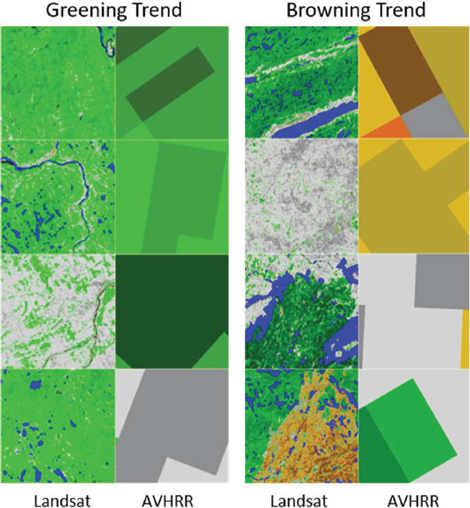
The Landsat record covers much of the same time period as AVHRR, and comparison of greening and browning trends between the two platforms was discussed throughout the workshop as a key example of the challenge in reconciling observations across methodological approaches. Research has shown that areas of greening broadly agree between AVHRR and Landsat (Ju and Masek, 2016), but discrepancies have been identified. For example, multiple attendees noted that Landsat shows a greening trend in eastern Canada in the 1984-2012 time period that is not captured in the AVHRR GAC dataset. In general, the lower resolution of AVHRR data cannot capture finer-grain landscape complexity or heterogeneity observed in Landsat data (see Figure 5).
MODIS MAIAC
Alexei Lyapustin, NASA Goddard Space Flight Center, provided an overview of the latest Multi-Angle Implementation of Atmospheric Correction (MAIAC) dataset from the Moderate Resolution Imaging Spectroradiometer (MODIS) satellite platform. The MAIAC dataset represents a significant improvement in cloud and snow detection and aerosol retrieval accuracy, which translates to increased accuracy in estimates of surface reflectance. There is also an increase in the number of retrievals in partly cloudy conditions, including at northern latitudes. The calibration of MODIS data has been improved in Collection 6 (which was then processed using MAIAC) and in future collections, which is valuable for estimating NDVI trends. Measurement of EVI has also improved, and noise in the data has been reduced.
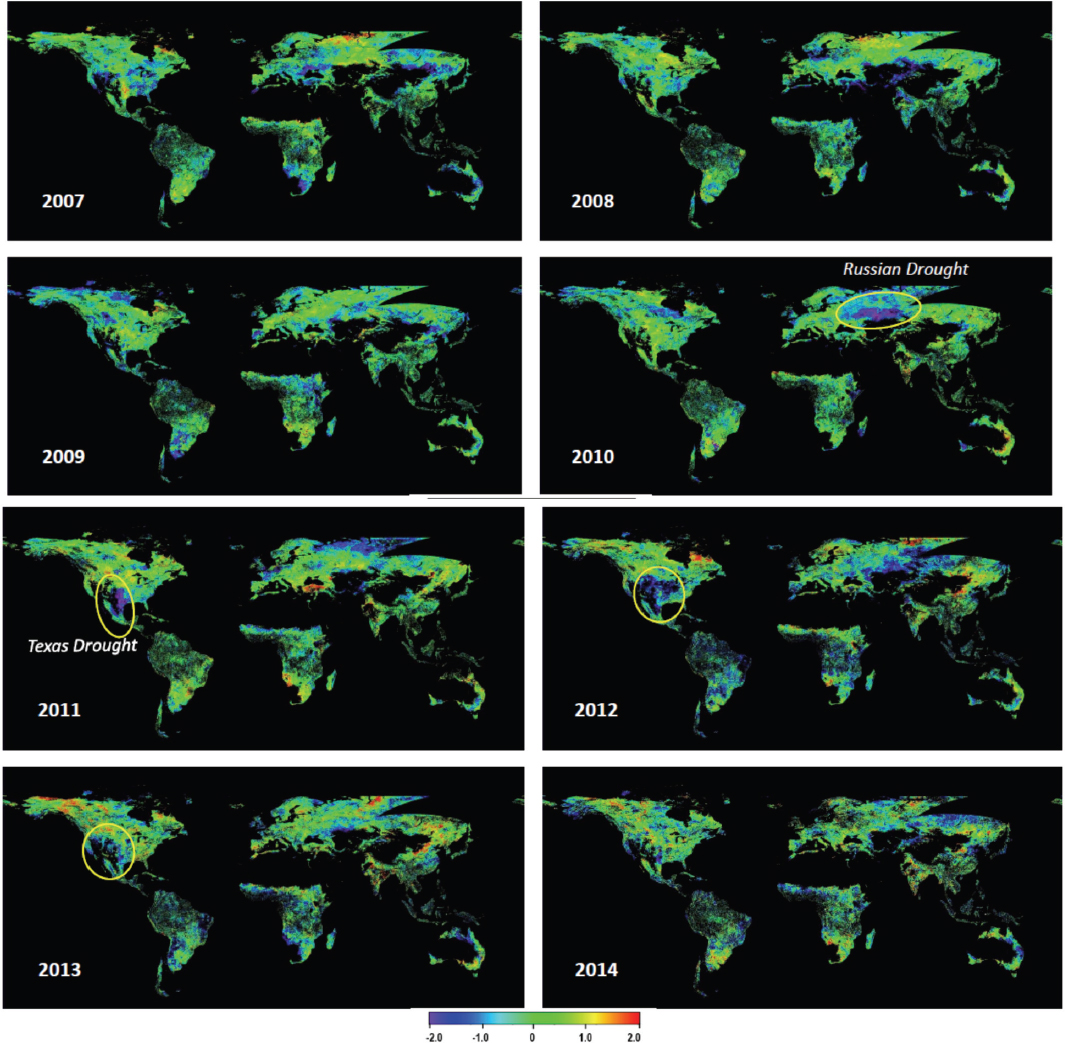
Lyapustin illustrated the use of MAIAC’s climate-modeling grid (approximately 5 km resolution) to evaluate global MaxNDVI using 2003 to 2010 as a baseline. He generated annual anomalies and computed 10-degree zonal mean summaries of greening and browning. Results showed relatively stable greenness around the globe except for the semi-arid regions where natural variations are very large. For NDVI anomalies across different years, a strong greening trend was observable in central Russia, Europe,
and Eastern Siberia. The Russian drought of 2010 and U.S. Texas drought of 2011-2012 generated strong negative anomalies, suggesting browning (see Figure 6). Considerable greening east of Hudson Bay in Canada and other Canadian locations were also observable most years between 2011 and 2017. For zonal mean averages, northern latitudes showed relatively high interannual variability but a clear trend toward greening. Evaluation for browning yielded little to no trend for the region.
NEW REMOTE SENSING TECHNOLOGIES TO STUDY GREENING AND BROWNING
In addition to the long records available from a number of remote sensing instruments, there are also new campaigns and technologies being adopted to evaluate greening and browning trends. These approaches can provide new types of data and can also serve to bridge gaps in spatial scales that exist among more traditional methodologies. One large effort noted by Goetz and other meeting participants is NASA’s ABoVE program. This includes data collections at various scales, including airborne campaigns, that are being used to address questions related to tundra and boreal greening and browning, among other topics.
Solar-Induced Fluorescence
SIF can provide information on greening and browning because it is viewed as a proxy for GPP that captures its spatial and temporal resolution, explained Xi Yang, University of Virginia. SIF data have been shown to correlate well with other GPP products at the global scale, and hotspots of fluorescence can be detected in high productivity regions including the tropics and the U.S. Midwest (Frankenberg et al., 2011). Seasonal patterns are also discernable, including low- to zero-SIF values in winter in cold regions when plants are largely inactive. At the site scale, Yang has also found that SIF is a good indicator of
seasonal and diurnal variation in vegetation activity in temperate forest (Yang et al., 2015). Preliminary results show a correlation between SIF and net photosynthesis for leaf-level measurements as well as comparison with estimates of GPP collected using the eddy covariance flux tower approach at Imnavait Creek, Alaska (see Eddy Covariance section for more detail on this method). Regional satellite SIF observations can also capture spring onset and fall senescence in the tundra region (Parazoo et al., 2018).
Absorbed photosynthetically active radiation (APAR) is the dominant driver of the relationship between SIF and GPP. Importantly, this APAR value includes only absorption by chlorophyll, whereas other measures of photosynthetically active radiation also include absorption by branches and stems. Each photon of light that enters a plant is either utilized as photosynthetic or fluorescence yield, or dissipated as heat. When photosynthetic yield is high, heat dissipation is low. Adding in consideration of fluorescence yield shows a positive correlation between fluorescence and photosynthetic yields during most daylight hours. Although this relationship has been demonstrated, it is not yet conclusive.
Airborne and satellite SIF observations are currently available for northern latitudes. The ABoVE campaign has a chlorophyll fluorescence imaging spectrometer with SIF measurements for 2017. Many satellites also provide SIF data, although years of availability are relatively limited (see Table 1 for a list of satellites collecting SIF data). The Tropospheric Monitoring Instrument (TROPOMI) is of particular interest to the SIF community because it currently provides the highest temporal and spatial resolution data, beginning in 2018, and has the highest resolution.
Lidar, Hyperspectral, and Thermal Airborne Imager
Doug Morton, NASA Goddard Space Flight Center, stressed that airborne campaigns provide unique access to remote areas and allow for coincident, high-resolution measurements of numerous metrics that can inform understanding of vegetation change. He focused his remarks on NASA Goddard’s Lidar, Hyperspectral, and Thermal (G-LiHT) Airborne Imager. G-LiHT is a portable airborne imaging system that uses multiple instruments to simultaneously map the composition, structure, and function of terrestrial ecosystems. In this system, lidar provides 3-dimensional information about the forest canopy and topography and how it may be changing (e.g., in response to fire disturbance); visible and near infrared imaging spectroscopy can discern species composition and variations in biophysical variables (e.g., photosynthetic pigments); thermal imagery delineates wetlands and detects heat and moisture stress in vegetation; stereo red, green, blue photographs capture fine-scale (~3 cm) canopy features; and SIF measurements provide actual photosynthetic activity and serve as an indicator of vegetation stress. Data are available at a 1 m resolution and are open access.1
G-LiHT has been used in interior Alaska to develop estimates of aboveground carbon stocks based on the ability to bridge the scale gaps between field-based forest inventory measurements and satellite data (e.g., Landsat) using hierarchical statistical modeling techniques. G-LiHT vegetation imagery has also been compared to historic high-resolution aerial photos to evaluate vegetation cover and height changes over time, and to look at how observed patterns may coincide with NDVI in the AVHRR and Landsat records. Using these 3-dimensional data can therefore help to disentangle greening and browning signals in the satellite record, and with repeated observations over time, Morton thinks G-LiHT data can lead to significant progress in understanding the mechanisms driving changes in Arctic and boreal vegetation.
___________________
Drones
Multiple presenters suggested that expanded use of drones could be a powerful approach to advance understanding and improve linkages of measurements across scales. Morton indicated an interest in capturing higher-resolution data using drones. He noted the particular value of higher resolution information in boreal forest because individual trees are generally very small. In recently burned areas, standing dead trees can be an important component of the landscape for decades that contribute to changes in successional trajectories, and these fine-scale features of forest structure can be captured using drone imagery. Deploying drones may also be a pathway to expand remote sensing coverage in remote regions to provide context for field measurements of vegetation in the absence of routine airborne campaigns, Morton explained. Meddens indicated that high-resolution drone imagery could allow for detection of tree-level mortality occurring with insect outbreaks that are currently undetectable at fine scale with satellite observations.
For tundra ecosystems, Isla Myers-Smith, University of Edinburgh, suggested that increased use of drone imagery could bring in landscape-scale information to address mismatches found in studies striving to link satellite and field-based measurements. Expanded use of drones is now under way through the High Latitude Drone Ecology Network.
A challenge to drone usage noted by Meddens is that the instruments cannot be flown beyond visual line of sight, which may limit their geographical use to more easily accessible sites. Other participants also discussed the infrequency with which repeat measurements would likely be taken without a large funding source.
FIELD-BASED MEASUREMENT OF GREENING AND BROWNING
Various metrics of plant productivity can be readily measured at plant to plot scales to identify greening and browning patterns and explore potential drivers of change, including those that may only be discernable at a local scale. These measurements can include evaluation of plant growth (above- and belowground), percentage cover of various species, changes in timing of plant leaf out and senescence (phenology), and nutrient cycling rates and gas fluxes, among others. Multiple presenters emphasized the importance of field-based data for validating findings of remote sensing studies, and as a result, field-based measurements were discussed throughout the workshop (see Table 1 for a list of techniques identified by workshop participants). This section provides more detail on just a few of the many available approaches.
Eddy Covariance
Elyn Humphreys, Carleton University, provided an overview of the eddy covariance method, which measures turbulent exchange of trace gases (often CO2) and energy (latent and sensible heat) between the atmosphere and Earth’s surface. The eddy covariance approach has been used for decades, and improvements in the instrumentation and technique now allow for year-round, long-term measurements to be collected. This method captures fluctuations in the vertical velocity of wind and correlates this information with the gas or energy metric of interest. Measurements can be collected continuously and provide flux estimates on a 30-minute timescale. Instrumentation is placed on towers that extend above the vegetation canopy. For every 1 m above the surface, the measurement captures gas exchange information from a footprint extending out about 100 m horizontally in the direction from which the wind is coming, with this distance varying greatly depending on surface roughness and
atmospheric stability. The approach works best when the tower is located on a flat, homogenous landscape.
Collection of supporting microclimate, ecosystem, and vegetation characteristics is key to interpreting underlying processes and trends associated with measured fluxes. Eddy covariance values represent a net ecosystem exchange (NEE), which differs from other field-based and remotely sensed productivity measurements discussed at the workshop. To allow for comparison with these other methods, models are applied that partition ecosystem respiration and photosynthesis. For instance, one can look at the flux measurements from the nighttime only (which represents only respiration) and use the relationship between these values and temperature to then model daytime respiration rates. The difference between the measured NEE and the modeled respiration provides an estimate of GPP. In the absence of darkness during the summer months at high latitudes, respiration can be estimated over a number of days using light response curves and these measurements are then related to background soil temperature or air temperature. With these metrics of plant productivity, researchers can then evaluate the relationship to greening and browning patterns that may be observed.
A primary strength of the eddy covariance method, Humphreys added, is that it allows for study of an ecosystem’s function as a carbon source or sink. This can then provide valuable insights into the source and sink strength of different vegetation types and changes over time. Challenges to this technique include a need to cross-correlate sensors and data processing techniques to ensure robust long-term time series and avoid false trends. Eddy covariance tower locations are also relatively sparse at northern high latitudes, and studies are often conducted for a relatively short number of years (or only during the snow-free seasons) and require synthesis efforts to explore regional and longer-term trends. However, Humphreys noted that the distribution of sites is expanding.


