3

Sea-Level Change

Sea level is a leading indicator of climate change because its long-term change is driven mainly by the amount of heat being absorbed by the oceans and the amount of land ice being melted by a warmer atmosphere and oceans. Monitoring sea-level changes at global to regional scales, understanding why it is changing, and projecting how sea level might change in the future are critical for mitigating adverse impacts on coastal infrastructure, ecosystems, and human society. A broad array of satellite observational systems, whose accuracy depends heavily on precise geodetic infrastructure, is required to observe and understand these changes and impacts.

Studies of sea level focus on (a) absolute sea-level change (sea level measured with respect to the Earth’s center of mass or other suitable reference surface), which is important for understanding climate change; and (b) relative sea level (sea level measured with respect to the land surface, which may itself be moving), which is important for assessing impacts along the coasts. The Decadal Survey (NASEM, 2018) describes the scientific needs for understanding both absolute and relative sea-level rise. This chapter examines what is needed from the geodetic infrastructure to help answer the important Decadal Survey science questions:

C-1. How much will sea level rise, globally and regionally, over the next decade and beyond, and what will be the role of ice sheets and ocean heat storage?

S-3. How will local sea level change along coastlines around the world in the next decade to century?

C-6. Can we significantly improve seasonal to decadal forecasts of societally relevant climate variables?

H-1. How is the water cycle changing? Are changes in evapotranspiration and precipitation accelerating, with greater rates of evapotranspiration and thereby precipitation, and how are these changes expressed in the space-time distribution of rainfall, snowfall, evapotranspiration, and the frequency and magnitude of extremes such as droughts and floods?

The geodetic infrastructure needs associated with these questions appear in the Sea-Level Change Science and Applications Traceability Matrix (see Appendix A, Table A.1).

SCIENCE OVERVIEW

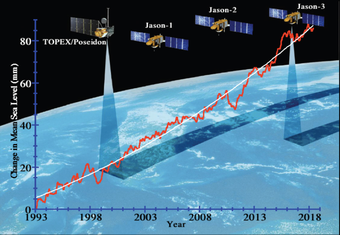
Sea-level science has been revolutionized by satellite observations because of their precision and near global coverage. Sea level has been monitored continuously over the past 27 years by a series of high-precision satellite altimetry missions (see Figure 3.1), which have been validated with tide gauge data. These records show that climate-driven global mean sea level has risen by 3.1 ± 0.3 mm/yr since 1993 and that the rate has accelerated by 0.084 ± 0.025 mm/yr² (Dieng et al., 2017; Nerem et al., 2018; WCRP Global Sea Level Budget Group, 2018).

An important goal of sea-level science is to determine not only how much sea level is changing, but why it is changing and the relative contributions of thermal expansion, melting of ice sheets and glaciers, and other factors. With this knowledge, we can better forecast how sea level will change in the future. Satellite gravity measurements from missions such as the Gravity

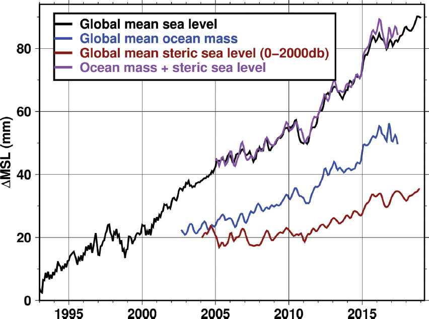
Recovery Climate Experiment (GRACE) have proven valuable in this regard, because they provide information on how much melting ice is contributing to sealevel change, as well as variability caused by land-ocean hydrologic exchanges. Melting of land ice is currently the largest contributor to sea-level rise (44 percent for 1993–2015 and 55 percent for 2005–2015; see WCRP Global Sea Level Budget group, 2018), followed by thermal expansion of the ocean due to ocean warming (see Figure 3.2). Changes in ocean heat content can be measured by differencing altimetric sea-level measurements with satellite gravity measurements of ocean mass. Ocean heat content change can also be measured with the Argo network of profiling floats, which have minimal dependence on the geodetic infrastructure.

Changes in land water storage cause considerable interannual variability in global mean sea-level change. Much of this variability is driven by precipitation changes associated with climate oscillations such as the El Niño–Southern Oscillation. While climate-driven changes in total land water storage are currently small, it is important to understand the interannual variations so that they can be separated from the forced response (ice melt and ocean expansion) due to climate change.

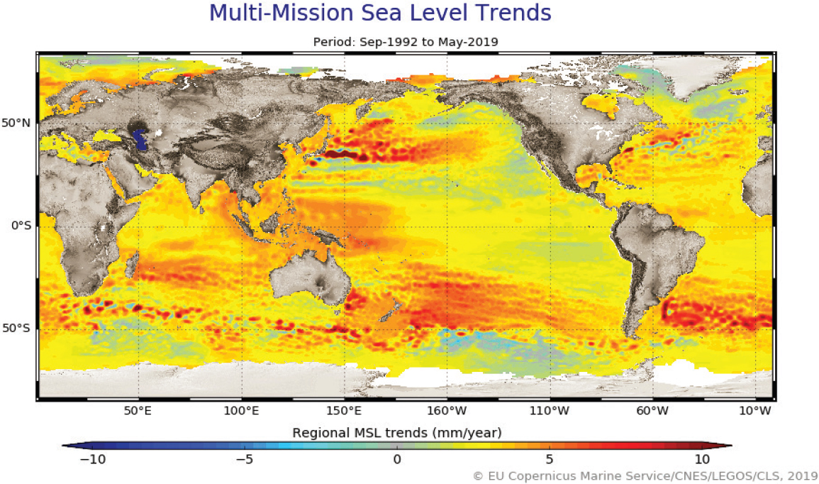
Satellite altimetry has revealed that the rates of sea-level change vary regionally (see Figure 3.3), driven primarily by ocean circulation and winds, which redistribute heat and fresh water, as well as by gravitationally driven patterns caused by melting ice. The latter also causes relative sea-level change due to vertical land motion in response to the deformation of the Earth from ancient and modern land ice melt. Recent research suggests the 26-year regional sea-level trends are dominated by the forced response due to climate

change, and that these patterns will continue into the future (Fasullo and Nerem, 2018). Therefore, the regional trends shown in Figure 3.3 provide insights on regional variations in future sea-level change.

Coastal sea level relative to the land surface is the quantity of most practical interest for understanding the societal impacts of sea-level change. Relative sea level depends on global mean sea-level rise and its regional variations, vertical land motion, and other local processes, such as small-scale currents, wind, waves, fresh water input from river estuaries, shelf bathymetry, and along-shore and cross-shore sediment transport (e.g., Woodworth et al., 2019).

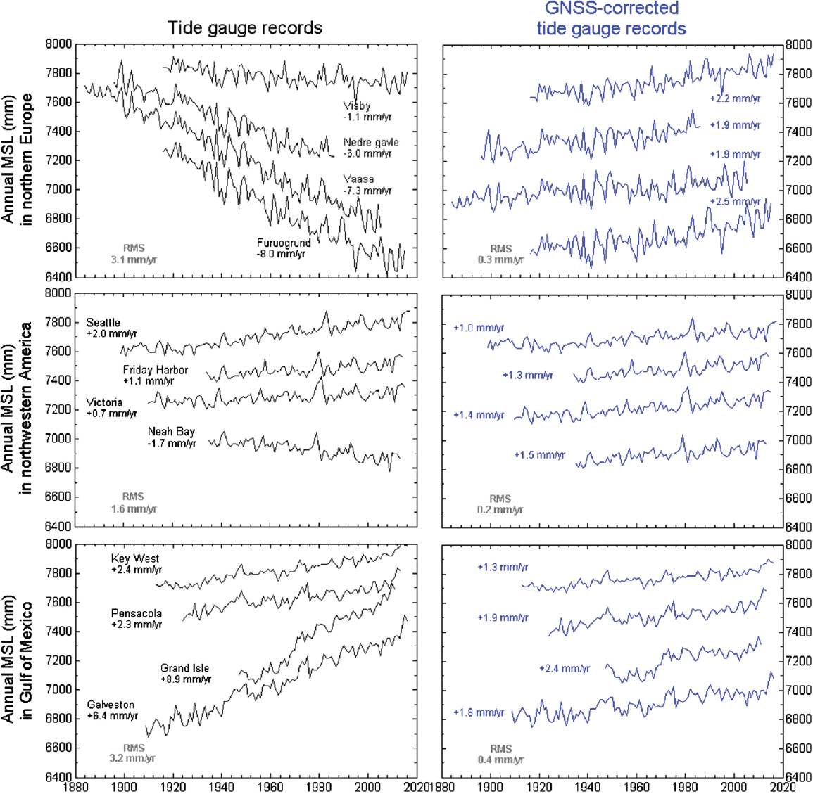
Along many coasts, land subsidence amplifies the impacts of climate-related sea-level rise. Consequently, measuring vertical land motion is important for assessing the societal impacts of sea-level change. Vertical land motions are caused by a variety of phenomena, including tectonic and volcanic deformations, ground subsidence due to natural processes (e.g., sediment loading in river deltas) or human activities (e.g., groundwater pumping in coastal megacities and oil and gas extraction on continental shelves (Woppelmann and Marcos, 2016). Figure 3.4 shows relative sealevel time series measured by tide gauges, before and after correcting for vertical land motions. The case of Galveston in the Gulf of Mexico is particularly interesting. The uncorrected tide gauge record indicates that relative sea level rose by 6.4 mm/yr since 1900, mostly due to ground subsidence caused by sediment compaction due to groundwater withdrawal.¹ After correcting for vertical land motion, the rate of sea-level rise in that area is reduced to 1.8 mm/yr.

The solid Earth response to melting land ice also gives rise to vertical land motion by two other mechanisms: (1) the viscoelastic response associated with the last deglaciation, called glacial isostatic adjustment (GIA), and (2) the elastic response associated with present-day land ice changes. These responses, mostly known from modeling, create complex re-

___________________

¹ See https://txpub.usgs.gov/houston_subsidence/home.

gional patterns in both absolute and relative sea-level change (Peltier, 2004; Tamisiea, 2011): sea level drops in the immediate vicinity of the melting land ice and rises in areas that were not covered by high volumes of ice during the last glacial maximum. GIA depends on the Earth’s mantle viscosity and deglaciation history (Peltier, 2004; Lambeck et al., 2010), whereas the response of the solid Earth to modern land ice melt depends on lithosphere elasticity and the amount and location of ice mass loss. The latter deforms the ocean floor and changes the Earth’s gravity field, resulting in a nonuniform pattern of sea-level rise, generally known as “sea-level fingerprints” (Mitrovica et al., 2009). Although decades of sea-level observations may be needed to routinely detect sea-level fingerprints, some fingerprints have already been detected (Hsu and Velicogna, 2017). As ice melt contributions from Greenland and Antarctica grow, regional sea-level trends will be dominated by the gravitational fingerprints of ice sheet mass loss.

GIA increases the volume of the ocean basins, producing a linear effect of ~–0.3 mm/yr on the altimetry-based record of global mean sea-level rise (Peltier, 2004; Tamisiea, 2011). GIA is usually considered a correction that needs to be subtracted from the global mean sea-level rise time series to estimate changes in water volume. Its uncertainty is estimated to be of the order of 0.15 mm/yr (Tamisiea, 2011). The effect of GIA on GRACE-based global mean ocean mass estimates is much more important (and must be corrected for), because it is on the same order of magnitude as the ocean mass change signal itself.

The response of the solid Earth to ancient and present-day ice loading needs to be better understood, because it is a leading source of error in GRACE estimates of ice mass loss from the ice sheets. Global Navigation Satellite System (GNSS) measurements of vertical and horizontal crustal motion are an important tool for improving GIA models, but they depend on an accurate terrestrial reference frame (TRF) so that the measurements are not biased or regionally distorted. GNSS measurements are also important for accurately measuring vertical land motions due to earthquakes (coseismic and postseismic) and local subsidence due

to hydrologic pumping, for example, so tide gauge measurements can be properly defined in the TRF.

SEA-LEVEL CHANGE

Sea level is measured by a constellation of altimeter satellites that enable near-global coverage. The height of the satellite above the ocean surface is converted to a sea-surface height (or sea level) above a reference surface determined from precise orbit determination. The estimated sea-surface height is then corrected for atmospheric (ionospheric and tropospheric) delays, biases between successive altimetry missions, and geophysical effects such as the sea state bias, solid Earth tides, and pole and ocean tides. With these corrections, satellite altimeter measurements have a point-to-point accuracy of a few

centimeters. The Topography Experiment (TOPEX)/Poseidon and Jason-1, -2, and -3 missions have provided a continuous record of sea-level change over ±66° latitude with a 10-day repeat period. The precision of global mean sea level for each 10-day average is about 4–5 mm.

Measurements

The Decadal Survey (NASEM, 2018) called for determining global mean sea-level rise to within 0.5 mm/year over the course of a decade (Objective C-1a) and regional sea-level change to within 1.5–2.5 mm/yr over the course of a decade (Objectives C-1d and S-3a). For the latter objective, 1.5 mm/yr corresponds to a ~6,000 km² region and 2.5 mm/yr corresponds to a ~4,000 km² region. Achieving these objectives will require measurements of sea-surface height with a sampling of 7 km along-track, every 10 days, and a precision of 30 mm at 7 km and 1 mm/yr globally. This requires satellite radar altimeter measurements (including water vapor radiometer measurements) and precise orbit determination of the satellites relative to a well-defined terrestrial reference frame.

Observations of relative sea-level variations along the coast are essential for understanding the processes at work and for evaluating the impacts of sea-level rise on coastal environments and infrastructure. The world’s coastal zones are severely undersampled by tide gauges and, until recently, were unsurveyed by conventional satellite altimeters within 15 km of the coast. Dedicated reprocessing of conventional nadir altimetry and use of innovative new observations from synthetic aperture radar technology (e.g., on Sentinel-3A/B) and wide swath altimetry would help fill some of these data gaps.

Tide gauge measurements provide one of the few records of sea-level change prior to the era of satellite altimetry. As such, they provide one of the only methods for placing the satellite record of sea-level change into a longer term context, although they can be influenced by vertical land motion. In addition, tide gauges are used to validate satellite altimetry and detect drifts in the satellite instruments (Mitchum, 2000). The error in the altimeter tide gauge validation is the leading error source for monitoring sea-level change with satellite altimetry. Thus, for both sea-level science and altimeter validation, it is important that the geodetic infrastructure include the means for monitoring vertical land motion at as many tide gauges as possible (Woodworth et al., 2017). The use of GNSS to validate altimetry measurements at tide gauge sites is described in Box 3.1.

Geodetic Needs

An accurate TRF and precision orbit are fundamental science requirements for satellite altimetry applications, such as sea-level change (Blewitt et al., 2010). The orbit accuracy is directly linked to the accuracy and stability of the TRF in which the orbit is computed. The performance of the tracking systems (Satellite Laser Ranging [SLR], Doppler Orbitography and Radiopositioning Integrated by Satellite, and GNSS) in terms of network coverage and atmospheric propagation corrections, the accuracy of the tracking station positions versus time, and the accuracy of the reference frame origin (geocenter motion) and Earth orientation parameters are all important. The radial orbit accuracy for satellites such as Jason-3 now approaches 10 mm RMS. Errors in the TRF map into the orbit, and through the orbit directly to the altimeter-based, sea-level measurement. Errors in the Z component of the geocenter are the most problematic, because they map directly into the orbit. The X/Y geocenter errors, which are modulated by the Earth’s rotation once per day relative to the satellite orbit, do not map directly into the orbit errors, and thus have minimal impact on the orbit. Orbit error remains the largest source of error in the altimetry system, although its amplitude has decreased over time due to improved Earth gravity models (from GRACE and Gravity field and steady-state Ocean Circulation Explorer observations). Despite this improvement, temporal changes in the gravity field, largely due to the melting ice sheets, can introduce biases into regional sea-level change measurement if not properly accounted for in the orbit determination process.

Satellite altimetry is potentially subject to instrument drifts that could masquerade as climate signals. For this reason, tide gauge measurements have been used to validate altimeter measurements (e.g., Mitchum, 2000). For estimates of the rate of sea-level rise from satellite altimetry, the error estimate derived from the tide gauge validation is driven by errors in the amount of vertical land motion at the tide gauge sites. Therefore, improved estimates of vertical land motion can reduce the error estimate for the rate of sea-level rise from satellite altimetry.

The geodetic needs associated with obtaining satellite measurements with an accuracy of 20 mm (after correction for tides and wave effects) and long-term measurement drift errors of less than 0.5 mm/yr over a decade are as follows:

• The tracking systems used for precision orbit determination need to support a radial orbit accuracy of at least 20 mm and tracking station position accuracy of 1 mm in the TRF.
• TRF accuracy of less than 1 mm at all times (i.e., the TRF must be maintained). It should always be possible to relate the reference frame in one year to the reference frame in another year so that sealevel changes from year to year can be accurately computed.
• Drifts in the TRF origin to an accuracy of less than 0.1 mm/yr.
• The TRF should be free of deformations that might cause errors in regional patterns of sea-level change.
• Vertical land motion accuracy at tide gauges of less than 0.5 mm/yr to minimize errors in validating satellite altimeter observations of sea-surface height.

THERMAL EXPANSION—OCEAN HEAT STORAGE

More than 90 percent of the heat trapped by greenhouse gas emissions since the Industrial Revolution is stored in the ocean (Cheng et al., 2017). Determining the ocean heat storage change is important for assessing the current state of climate and how it may change in the future. The difference between altimeter measurements of sea-level change and satellite gravity measurements of changes in ocean mass (due to land-ocean water/ice exchanges) provides an estimate of the global mean steric sea level associated with thermal expansion, from which the full-depth ocean heat content can be estimated (Levitus et al., 2005; Melet and Meyssignac, 2015).

Thermosteric sea level and ocean heat storage can also be estimated from the Argo array of profiling floats. The present array measures heat storage only in the upper 2,000 m of the global oceans, creating uncertainty in estimates of the total ocean heat storage (Purkey and Johnson, 2010; Johnson et al., 2015). Expanding the Argo array to sample the deep ocean would improve understanding of total ocean heat storage and the heat exchange between the upper and deeper ocean, and improve forecasts of oceanic heat uptake and expansion. It would also improve validation of altimetry and GRACE systems.

Measurements

Measurements of the change in the global oceanic heat uptake are needed to within 0.1 W/m² over the course of a decade (Objective C1-b). Achieving this objective will require measurements of sea-surface height, ocean mass distribution, and in situ measurements of temperature and salinity (Argo floats that employ satellite links for data transmission and data localization). Altimetry measurements need to be acquired with a sampling of 7 km along-track, every 10 days, precision of 30 mm at 7 km 1 mm/yr globally. These requirements can be met with a radar altimeter, a microwave radiometer, and precision orbit determination of the satellite carrying these instruments.

For ocean mass distribution, monthly gravity measurements with 300 km × 300 km spatial resolution, a stability of 15 mm water equivalent at 300 km × 300 km, and precision in ocean mass change of 0.1 mm/decade. Globally averaged ocean mass from satellite gravity measurements is very sensitive to errors in the GIA model employed (Tamisiea, 2011). Ocean temperature and salinity measurements are needed for every 3 degree × 3 degree grid, every 10 days, with an accuracy of 0.01 degrees and 0.01 practical salinity units. These measurement requirements can be met by maintaining the core Argo float program and developing the deep Argo float program.

Geodetic Needs

Same as “Sea-Level Change.”

ICE SHEETS AND GLACIER MASS CHANGES

Glaciers and ice sheets represent the largest uncertainty in sea-level projections and will soon dominate the pattern of regional sea-level change. Three main approaches for measuring ice sheet mass changes are based on satellite observations that depend on the geodetic infrastructure. First, time series of time-variable gravity measured by GRACE have proven invaluable for measuring the total changes in the mass of ice sheets (see Figure 3.6), glaciers, and ice caps at coarse spatial

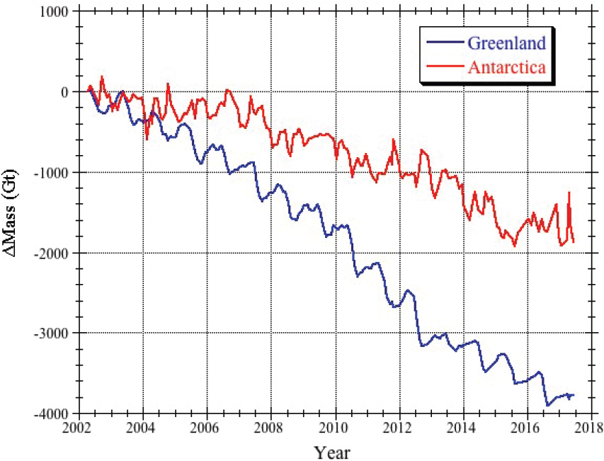
resolution. Limitations of GRACE include its short temporal record and the need to correct the measurements for land hydrology and GIA to isolate the ice mass change signal. In addition, GRACE cannot measure the mass change signal associated with spherical harmonic degree 1 (the geocenter motion), and some degree 2 and 3 terms have large errors. These must be estimated from other techniques, such as SLR.

The second approach involves measurements of ice motion and grounding line positions from Interferometric Synthetic Aperture Radar (InSAR). Ice motion measurements are essential for documenting changes in ice dynamics and for understanding processes, such as how glaciers react to climate forcing, which parts of the ice sheets are changing and how rapidly, and what fraction of the mass loss is controlled by glacier speed. Precise geocoding and knowledge of satellite orbits, which are essential for making quality observations, require a precise geodetic framework, but does not require the same accuracy as other techniques.

The third approach involves estimating ice mass changes from radar and laser altimetry measurements of elevation changes. The instrument requirements are similar to those for ocean applications and so are the constraints placed on the quality of the geodetic infrastructure. The laser and radar altimeters rely on precise determination of the satellite orbits (20 mm radially) to maintain a high precision determination of the height of the snow or ice surface. The measurements are sensitive to surface slope, and so multiple beams and precise georeferencing of the laser pointing or interferometric processing of the radar altimeter data are required in coastal areas with steep slopes. The results must be corrected for the GIA. Uncertainties remain in the interpretability of the mass change signal since the density of the ice/snow must be known to determine mass changes from elevation changes.

Measurements

Objective C-1c is to determine the changes in total ice-sheet mass balance to within 15 Gton/yr over the course of a decade and the changes in surface mass balance and glacier ice discharge with the same accuracy over all of the ice sheets, continuously, for decades

to come. The relevant measurements are ice sheet mass, velocity, surface and bed elevation, and thickness, as well as ice shelf (floating land ice) thickness and cavity shapes.

Determining ice sheet mass balance requires monthly gravity measurements at the basin scale and a precision of 10 mm water equivalent or better on spatial scales of a few hundred km. These measurements are already provided by GRACE and will be improved and extended with GRACE-FO and with supplemental geodetic measurements for GIA corrections.

Ice sheet velocity needs to be measured with weekly to daily samples every 100 m pole to pole, a precision of 1 m/yr in fast flow areas and 0.1 m/yr in the interior. The necessary precision can be achieved with InSAR for fast flow and interior regions and with high-resolution optical sensors for fast flow areas only. The same measurements should provide information on grounding line position with a sampling of 100 m pole to pole, and a vertical motion precision of 5 mm, which can be achieved with InSAR.

Measurements of ice sheet elevation are needed with weekly to daily sampling, vertical resolution of 0.1–0.2 m, along-track resolution of 100 m, and across-track resolution better than 1 km. These requirements can be met with a multi-beam laser altimeter. At present, Ice, Cloud, and land Elevation Satellite-2 provides better than 0.1 m vertical resolution, 70 m along-track resolution, and 3 km across-track resolution (Kwok et al., 2019).

Measurements of ice sheet thickness and ice shelf thickness are needed with a vertical precision of 10 m, horizontal spacing of 100 m pole to pole, and yearly sampling. These requirements can be met with suborbital radar sounders, laser altimetry (ice shelf only), high resolution optical sensors with stereo capability, and algorithms (mass conservation) that require information on ice velocity, surface velocity, and changes in surface height to interpolate in between radar sounding tracks on land ice.

Geodetic Needs

The GRACE mass change measurements strongly depend on the geodetic infrastructure. The determination of the geocenter is directly linked to the realization of the TRF origin. At present, degree-one spherical harmonic contributions (geocenter motion, due to the motion of the Earth’s center of mass with respect to the TRF) are calculated using GRACE-based gravity field variations and model-based assumptions on water mass redistribution in the global ocean (Swenson et al., 2008). However, geodetic techniques used to realize the TRF, particularly SLR (GNSS is also showing promise in this area), can be used to determine the geocenter motion independently. Given that the geocenter motion is one of the largest sources of uncertainty in GRACE-based surface mass change estimates (e.g., Blazquez et al., 2018), it is important to maintain the geodetic infrastructure to improve these parameters (also involved in the orbit precision; see above).

The geodetic requirements for ice sheet altimetry are the same as those discussed in “Sea-Level Change.” For interferometry, the tracking systems used for precision orbit determination should support a three-dimensional orbit precision of less than 0.1 m, and the tracking station positions should be known to 1 mm in the TRF. In addition, the TRF should be known to <1 mm at all times (i.e., maintain the TRF). The geodetic infrastructure should also support determination of ionosphere and water vapor delays so that InSAR measurements can be corrected for atmospheric effects.

LAND WATER HYDROLOGY

Water on land is stored in different reservoirs, including rivers, lakes, wetlands, upper soil, and aquifers. Because of water mass conservation, changes in terrestrial water storage have an impact on the global mean sea level, but mainly at interannual frequencies. These changes have two main causes: (1) natural climate variability, in particular El Niño–Southern Oscillation events, and (2) human activities, such as dam construction, groundwater extraction, deforestation, and wetland conversion. GRACE observations of net land water storage are available since 2002 (Llovel et al., 2010; Reager et al., 2016; Scanlon et al., 2018). However, uncertainties are relatively high due to the coarse resolution of GRACE (~300 km) and the associated leakage of unrelated signals (e.g., nearby glaciers). The land water contribution to sea-level change can also be estimated using global hydrological models, but these models are also uncertain due to errors in the meteorological forcing and imperfect representation of human activities. Improvement is expected from assimilating GRACE data into the models (Döll et al., 2017). As

with the other contributions based on GRACE, GIA and geocenter motion issues are central and rely on a precise TRF.

In the near future, wide swath interferometric altimeters such as Surface Water Ocean Topography will provide novel constraints on lake levels, river discharge, and temporal changes in water storage. In addition, InSAR will observe land water withdrawal (subsidence), a major hazard caused by human activities, landslides, volcanoes, and earthquakes.These interferometric techniques impose significant requirements on the geodetic infrastructure.

Measurements and Geodetic Needs

Same as “Ice Sheets and Glacier Mass Changes.”

VERTICAL LAND MOTION

Measuring vertical land motions along the coasts using GNSS and InSAR is of primary importance. Land motions have different origins, including tectonics, which may uplift coastal areas and so reduce relative sea-level rise (e.g., Oregon and Washington; NRC, 2012), or sediment compaction or extraction of groundwater or hydrocarbons, which may cause significant ground subsidence, and so amplify climate-related sea-level rise. GIA also causes vertical land movements, particularly in high-latitude regions. GNSS near tide gauges can be used to estimate vertical land motions, but less than 14 percent of Global Sea Level Observing System tide gauge stations are equipped with a permanent GNSS station (e.g., Ponte et al., 2019). Several studies have shown the benefit of using InSAR in different coastal environments (e.g., Brooks et al., 2007). Measuring vertical land motions at the coast strongly relies on the geodetic infrastructure.

Measurements

Objective S-3b calls for measurements of vertical land motion along the coast with an uncertainty of <1 mm/yr. In addition, Objective C-1c specifies measurements of vertical land motion within 100 m of the coast around the globe, with monthly temporal resolution, and an accuracy of 1 mm/yr.

Geodetic Needs

Ideally, vertical land motion near tide gauges would be measured using GNSS receivers co-located with the tide gauges. In addition, GNSS reflection techniques should be investigated as an alternative means for measuring sea level and vertical crustal motion simultaneously. GNSS and InSAR are needed to map vertical crustal motion along the coasts.

SUMMARY

Satellite altimetry and satellite gravity are the main tools used by sea-level scientists that depend most strongly on the geodetic infrastructure. These measurements require a TRF that is precisely defined as a function of time. The TRF needs to have a precisely defined origin and be free of drifts and deformations, lest they create errors in the satellite measurements that could be misinterpreted as climate signals. Deformation of the TRF occurs when a fiducial site (or a regional group of fiducial sites) behaves in a nonlinear manner (caused by, for example, a melting ice sheet, earthquakes, or other nonlinear phenomena) that is not represented by the linear TRF models currently in use. This will become particularly challenging as the Earth’s shape and gravity field change due to climate change. Of particular concern is the movement of the Earth’s center of mass relative to its center of figure as the ice sheets melt, which could amount to several cm over a century. In addition, geodetic sites near areas of ice mass loss may show anomalous motion and should be treated carefully if used to define the reference frame. It is also important to always be able to reconstruct the TRF back in time, so that sea-level measurements made a century from now can be compared to sea-level measurements made today and to sea-level measurements made 25 years ago. This is generally referred to as maintaining the TRF.

Both satellite altimetry and satellite gravity require precision orbit determination. Onboard GNSS receivers can provide sufficient accuracy, but SLR is useful as a backup technique in case of failure of the GNSS receiver as well as for validating the orbit accuracy. The positions of GNSS and SLR tracking stations must be known precisely in the TRF.

The ITRF may not have sufficient accuracy for sea-level science in the future. As the Earth responds to climate change, the motion of the fiducial sites that comprise the TRF may depart significantly from the linear behavior currently assumed in the TRF definition. In addition, the geocenter will also respond to

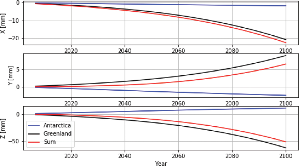
climate change, especially the melting of the ice sheets (see Figure 3.7). Research is needed on how to maintain the accuracy of the TRF in an era when the Earth is experiencing profound changes. This could include, for example, site characterization and modeling nonlinear motions of the TRF or locations of fiducial sites. It has also been proposed that a space-based collocation experiment could provide further improvements.

One area where the geodetic infrastructure could be improved is the monitoring of tide gauge positions using GNSS. Reducing the errors in vertical land motion for the tide gauge calibration of satellite altimeter measurements could significantly improve the error estimates for sea-level change from satellite altimetry. The following summarizes the needs for maintaining or enhancing the geodetic infrastructure, and related improvements to enhance scientific returns.

Maintenance of the Geodetic Infrastructure

• Maintain and enhance the geodetic infrastructure to achieve the TRF requirements as described below.
• Maintain the tide gauge record to validate the satellite altimetry data in order to achieve 0.1 mm/yr in the altimeter measurements averaged over a decade.
• The orbit determination requirements for altimetric satellites are 10–20 mm radial position. Three-dimensional orbit accuracy of better than 0.1 m is required for ice-sheet flow-rate measurements using InSAR.
• Maintain the current accuracy of the low degree and order geopotential field.
• Maintain and enhance the ancillary models and corrections for the altimetric satellites, including time-variable gravity, time-variable surface deformation, and atmospheric and ionospheric propagation models.

Enhancements to the Geodetic Infrastructure

• The sea-level science questions require a TRF accuracy of 1 mm and drift in the origin of the TRF of less than 0.1 mm/yr (or less than 0.02 ppb/yr in scale rate equivalent). Meeting these requirements would allow global sea-level rise to be determined to an accuracy of better than 0.5 mm/yr over the course of a decade and regional sea-level rise to within 1.5–2.5 mm/yr over the course of a decade. The definition of the Earth’s center of mass, especially in the Z-component, is especially dependent on successful tracking of SLR in the southern hemisphere.
• The signals in the motion of the Earth center of mass are expected to vary by as much as 50 mm in the next 100 years. There must be commensurate stability of

• the reference points for metrology at the fundamental sites, such as the invariant points of SLR telescopes or Very Long Baseline Interferometry dishes, or the GNSS monumentation. This may require studies on the stability and longevity of monumentation and drifts or stability of the tracking equipment.

• Install GNSS stations at tide gauges to achieve the absolute vertical land motion requirement of better than 0.5 mm/yr to minimize errors in validating satellite altimeter observations of sea-surface height. Encourage use of GNSS reflectometry methods to expand the number of worldwide tide gauges defined in the ITRF.

Related Improvements to the Geodetic Infrastructure to Enhance Scientific Returns

• Enhance the shallow water tide models to better connect the offshore altimetric heights with the coastal tide gauges.
• Develop software tools and automated handling for processing and integrating the diverse geodetic data sets used to investigate sea level.

REFERENCES

Melet, A., and B. Meyssignac. 2015. Explaining the Spread in global mean thermosteric sea level rise in CMIP5 climate models. Journal of Climate 28(24):9918-9940.

Mitchum, G.T. 2000. An improved calibration of satellite altimetric heights using tide gauge sea levels with adjustment for land motion. Marine Geodesy 23(3):145-166.

Mitrovica, J.X., N. Gomez, and P.U. Clark. 2009. The sea-level fingerprint of West Antarctic collapse. Science 323(5915):753.

NASEM (National Academies of Sciences, Engineering, and Medicine). 2018. Thriving on Our Changing Planet: A Decadal Strategy for Earth Observation from Space. Washington, DC: The National Academies Press.

Nerem, R.S., B.D. Beckley, J.T. Fasullo, B.D. Hamlington, D. Masters, and G.T. Mitchum. 2018. Climate-change-driven accelerated sea-level rise detected in the altimeter era. Proceedings of the National Academy of Sciences of the United States of America 115(9):2022-2025.

NRC (National Research Council). 2012. Sea-Level Rise for the Coasts of California, Oregon, and Washington: Past, Present, and Future. Washington, DC: The National Academies Press.

Peltier, W.R. 2004. Global glacial isostasy and the surface of the ice-age Earth: The ICE-5G (VM2) model and GRACE. Annual Review of Earth and Planetary Sciences 32:111.

Ponte, R.M., M. Carson, M. Cirano, C.M. Domingues, S. Jevrejeva, M. Marcos, G. Mitchum, R.S.W. van de Wal, P.L. Woodworth, M. Ablain, F. Ardhuin, V. Ballu, M. Becker, J. Benveniste, F. Birol, E. Bradshaw, A. Cazenave, P. De Mey-Frémaux, F. Durand, T. Ezer, L. Fu, I. Fukumori, K. Gordon, M. Gravelle, S.M. Griffies, W. Han, A. Hibbert, C.W. Hughes, D. Idier, V.H. Kourafalou, C.M. Little, A. Matthews, A. Melet, M. Merrifield, B. Meyssignac, S. Minobe, T. Penduff, N. Picot, C. Piecuch, R.D. Ray, L. Rickards, A. Santamaría-Gómez, D. Stammer, J. Staneva, L. Testut, K. Thompson, P. Thompson, S. Vignudelli, J. Williams, S.D.P. Williams, G. Wöppelmann, L. Zanna, and X. Zhang. 2019. Towards comprehensive observing and modeling systems for monitoring and predicting regional to coastal sea level. Frontiers in Marine Sciences 6. http://doi.org/10.3389/fmars.2019.00437.

Purkey, S., and G.C. Johnson. 2010. Warming of global abyssal and deep southern ocean waters between the 1990s and 2000s: Contributions to global heat and sea level rise budget. Journal of Climate 23:6336-6351.

Reager, J.T., A.S. Gardner, J.S. Famiglietti, D.N. Wiese, A. Eicker, and M.-H. Lo. 2016. A decade of sea level rise slowed by climate-driven hydrology. Science 351(6274):699-703.

Scanlon, B.R., Z. Zhang, H. Save, A.Y. Sun, H. Müller Schmied, L.P.H. van Beek, D.N. Wiese, Y. Wada, D. Long, R.C. Reedy, L. Longuevergne, P. Döll, and M.F.P. Bierkens. 2018. Global models underestimate large decadal declining and rising water storage trends relative to GRACE satellite data. Proceedings of the National Academy of Sciences of the United States of America 115(6):E1080-E1089.

Swenson, S., D. Chambers, and J. Wahr. 2008. Estimating geocenter variations from a combination of GRACE and ocean model output. Journal of Geophysical Research: Solid Earth 113(B8):B08410.

Tamisiea, M.E. 2011. Ongoing glacial isostatic contributions to observations of sea level change. Geophysical Journal International 186(3):1036-1044.

Watkins, M.M., D.N. Wiese, D.-N. Yuan, C. Boening, and F.W. Landerer. 2015. Improved methods for observing Earth’s time variable mass distribution with GRACE using spherical cap mascons. Journal of Geophysical Research (Solid Earth) 120:2648-2671.

WCRP (World Climate Research Programme) Global Sea Level Budget Group. 2018. Global sea level budget, 1993-present. Earth System Science Data 10:1551-1590.

Woodworth, P.L. G. Wöppelmann, M. Marcos, M. Gravelle, and R.M. Bingley. 2017. Why we must tie satellite positioning to tide gauge data. Eos, Transactions, American Geophysical Union 98. https://doi.org/10.1029/2017EO064037.

Woodworth, P., A. Melet, M. Marcos, R.D. Ray, G. Wöppelmann, Y.N. Sasaki, M. Cirano, A. Hibbert, J.M. Huthnance, S. Monserrat, and M.A. Merrifield. 2019. Forcing factors causing sea level changes at the coast. Surveys in Geophysics 40(6):1351-1397.

REFERENCES

Adhikari, S., E.R. Ivins, and E. Larour. 2015. ISSM-SESAW v1.0: Mesh-based computation of gravitationally consistent sea level and geodetic signatures caused by cryosphere and climate driven mass change [Data set]. https://doi.org/10.5194/gmdd-8-9769-2015.
Altamimi, Z., P. Rebischung, X. Collilieux, L. Métivier, and K. Chanard. 2019. Review of reference frame representations for a deformable Earth. International Association of Geodesy Symposia, pp. 1-6. https://doi.org/10.1007/1345_2019_66.
Beckley, B.D., F.G. Lemoine, S.B. Luthcke, R.D. Ray, and N.P. Zelensky. 2007. A reassessment of global and regional mean sea level trends from TOPEX and Jason-1 altimetry based on revised reference frame and orbits. Geophysical Research Letters 34(14):L14608.
Blazquez, A., B. Meyssignac, J.M. Lemoine, E. Berthier, A. Ribes, and A. Cazenave. 2018. Exploring the uncertainty in GRACE estimates of the mass redistributions at the Earth surface: Implications for the global water and sea level budgets. Geophysical Journal International 215(1):415-430.
Blewitt, G., Z. Altamimi, J. Davis, R. Gross, C.-Y. Kuo, F.G. Lemoine, A.W. Moore, R.E. Neilan, H.-P. Plag, M. Rothacher, C.K. Shum, M.G. Sideris, T. Schöne, P. Tregoning, and S. Zerbini. 2010. Geodetic observations and global reference frame contributions to understanding sea level rise and variability. In Understanding Sea-Level Rise and Variability, J.A. Church, P.L. Woodworth, T. Aarup, and W.S. Wilson, eds. Hoboken, NJ: Wiley-Blackwell. Pp. 256-284.
Brooks, B.A., M.A. Merrifield, J. Foster, C.L. Werner, F. Gomez, M. Bevis, and S. Gill. 2007. Space geodetic determination of spatial variability in relative sea level change, Los Angeles basin. Geophysical Research Letters 34(1):L01611.
Cheng, L., K.E. Trenberth, J. Fasullo, T. Boyer, J. Abraham, and J. Zhu. 2017. Improved estimates of ocean heat content from 1960 to 2015. Science Advances 3(3):e1601545.
Dieng, H.B, A. Cazenave, B. Meyssignac, and M. Ablain. 2017. New estimate of the current rate of sea level rise from a sea level budget approach. Geophysical Research Letters 44(8):3744-3751.
Döll, P., H. Douville, A. Güntner, H. Müller Schmied, and Y. Wada. 2017. Modelling freshwater resources at the global scale: Challenges and prospects. Surveys in Geophysics 37:195-221.
Fasullo, J.T., and R.S. Nerem. 2018. Altimeter-era emergence of the patterns of forced sea-level rise in climate models and implications for the future. Proceedings of the National Academy of Sciences of the United States of America 115(51):12944-12949.
Hsu, C., and I. Velicogna. 2017. Detection of sea level fingerprints derived from GRACE gravity data. Geophysical Research Letters 44(17):8953-8961.
Johnson, G.C., J.M. Lyman, and S.G. Purkey. 2015. Informing deep Argo array design using Argo and full-depth hydrographic section data. Journal of Atmospheric and Oceanic Technology 32(11):2187-2198.
Kwok, R., S. Kacimi, T. Markus, N.T. Kurtz, M. Studinger, J.G. Sonntag, S.S. Manizade, L.N. Boisvert, and J.P. Harbeck. 2019. ICESat-2 surface height and sea ice freeboard assessed with ATM lidar acquisitions from Operation IceBridge. Geophysical Research Letters 46(20):11228-11236.
Lambeck, K., C.D. Woodroffe, F. Antonioli, M. Anzidei, W.R. Gehrels, J. Laborel, and A.J. Wright. 2010. Paleoenvironmental records, geophysical modelling and reconstruction of sea level trends and variability on centennial and longer time scales. In Understanding Sea Level Rise and Variability, J.A. Church, P.L. Woodworth, T. Aarup, and W.S. Wilson, eds. Hoboken, NJ: Wiley-Blackwell. Pp. 61-121.
Larson, K.M. 2019. Unanticipated uses of the Global Positioning System. Annual Review of Earth and Planetary Sciences 47:19-40.
Larson, K.M., J.S. Löfgren, and R. Haas. 2013. Coastal sea level measurements using a single geodetic GPS receiver. Advances in Space Research 51:1301-1310.
Larson, K.M., J. Wahr, and P. Kuipers Munneke. 2015. Constraints on snow accumulation and firn density in Greenland using GPS receivers. Journal of Glaciology 61(225):101-115.
Larson, K.M., R.D. Ray, and R.D. Williams. 2017. A 10-year comparison of water levels measured with a geodetic GPS receiver versus a conventional tide gauge. Journal of Atmospheric and Ocean Technology 34:295-307.
Leuliette, E.W., and R.S. Nerem. 2016. Contributions of Greenland and Antarctica to global and regional sea level change. Oceanography 29(4):154-159.
Levitus, S. 2005. Warming of the world ocean, 1955-2003. Geophysical Research Letters 32(2):L02604.
Llovel, W., S. Guinehut, and A. Cazenave. 2010. Regional and interannual variability in sea level over 2002-2009 based on satellite altimetry, Argo float data and GRACE ocean mass. Ocean Dynamics 60(5):1193-1204.