
2
Air Quality
This chapter discusses wind erosion processes at Owens Lake that contribute to airborne particulate matter in the Owens Valley, air quality monitoring at Owens Lake, approaches for estimating PM10 emissions, and air quality modeling conducted as a part of developing a State Implementation Plan (SIP) to attain National Ambient Air Quality Standards (NAAQS) for particulate matter with an aerodynamic diameter of 10 micrometers or less (µm; PM10). Those topics are important for understanding the impact of dust control measures (DCMs) on airborne PM10 concentrations and making progress toward attainment of the NAAQS.
DUST GENERATION VIA WIND EROSION
Wind erosion results when the atmosphere in motion (wind) interacts with the granular media (sediments) on Earth’s surface. It affects more than 500 million hectares of land worldwide and results in 2 billion tons of dust emissions annually (Shao et al., 2011). Fugitive dust is often the most visible evidence of wind erosion and has detrimental impacts on commerce, air quality, and human health.
Earth’s surface exerts a drag on wind flow that results in shear forces capable of lifting and transporting sediment particles on the surface once the threshold wind velocity for that surface has been exceeded. Natural turbulence in the atmospheric boundary layer at the surface, caused by physical obstructions and convective overturn, results in wind gusts and lulls that often vary significantly from mean wind speeds. As the force of wind varies with the square of the wind speed, the shear forces near the surface will also vary, to a greater extent, along with incident wind speed. In addition, for mean 2-minute wind speeds in excess of 12 m/s (26.8 mph), the instantaneous wind speed in the 1 cm layer above the surface will exceed the 2-minute mean wind speed at least 5 percent of the time, resulting in very high shear stresses on surface particles (Van Pelt et al., 2006). For this reason, just a few extreme wind events often result in the predominance of soil redistribution and dust emissions at a given location. For instance, at a location in the Southern High Plains of North America, detailed wind erosion data were taken for 172 wind events during a 9-year period. Analysis of those data revealed that a single event was responsible for 8 percent of total soil loss, the most intense 10 percent of storms (17) accounted
for 50 percent of the total soil loss, and the most intense 50 percent of storms (86) resulted in 93 percent of the total soil loss measured during the time period (Van Pelt et al., 2006).
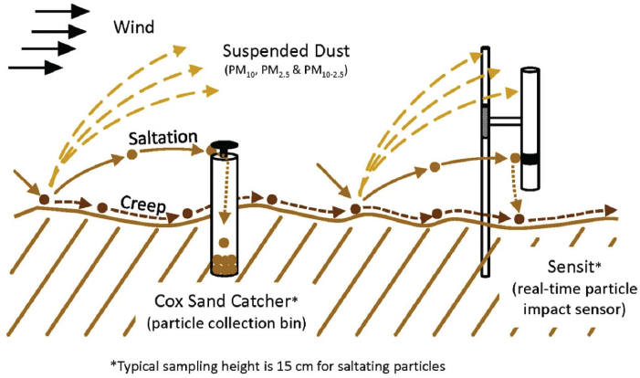
Wind-entrained particles move in three phases: creep, saltation, and suspension (Bagnold, 1941) (see Figure 2-1). In general, particles and aggregates larger than 840 µm in diameter are considered unerodable, but such particles and aggregates may be forced over the surface in very high velocity wind events. These larger particles and aggregates are in creep mode, because they do not leave the surface to be accelerated by the wind.
Saltation and suspension processes cause particles and aggregates to become airborne. For the saltation process, particles are lifted by shear forces into the air, accelerated by the wind, and return by gravity to the surface with a velocity-augmented impact energy. When saltating particles strike the surface, they may bounce, eject more particles and thus increase saltation, or abrade fine suspension-sized particles from crusted surfaces or aggregates (Shao, 2001).
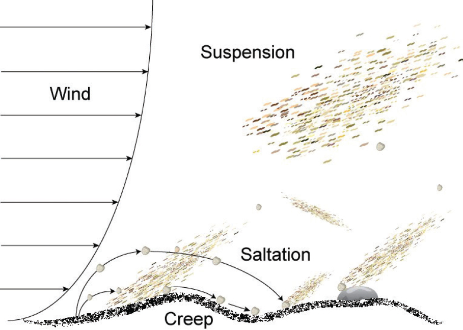
NOTES: The arrows on the left represent relative wind speeds and show the logarithmic decrease of velocity near the surface. Larger particles and aggregates move in creep mode, fine– and medium sand–sized particles move in saltation mode, and smaller particles enter true suspension and are transported away from the source by the wind. Particles are not drawn to scale.
SOURCE: Zobeck and Van Pelt, 2011.
Suspension occurs when smaller particles are directly entrained (emitted) into the air. Once airborne, the particles can be transported over long distances.
The absolute particle diameter separating saltation and suspension is determined by the velocity of the wind, but in general, the separation has been proposed to be in the range of 100 µm (Hagen et al., 2010) or smaller but almost always in the diameter range for very fine sand, with smaller particles becoming airborne via suspension. Particles or aggregates larger than 100 µm in diameter (primarily fine and medium sand) move via saltation. Therefore, sediments can contribute to airborne PM10 concentration through direct suspension of loose PM10 in surface sediments created by weathering and mechanical forces, abrasion of immobile aggregates and crusts by saltation impacts, and breakage of mobile saltation and creep-sized aggregates and particles into suspension size.
Field studies have shown that much of the coarser fraction of particles in the suspension mode are deposited on the surface within a few hundred meters of their source (Hagen et al., 2007). The finer portions, including PM10, may be lofted to great altitudes and transported hundreds or thousands of kilometers before returning to Earth’s surface (Cahill et al., 1994; Shao et al., 2011).
EFFECTS OF SEASONALITY ON DUST EMISSIONS AT OWENS LAKE
The climate of the Owens Valley is similar to many arid and semi-arid regions of the world, with summer temperatures often exceeding 100°F and winter temperatures commonly below freezing at night. Winds in the Owens Lake vicinity are generally from the north or south, although strong westerly winds can occur. However wind direction and wind speed are highly variable. Winds can be generated by synoptic storms, as well as local summer convection storms. Duell (1990) reports wind speeds in excess of 30 mph are not uncommon. Danskin (1998) reports that elevated winds can occur at any time of the year but are often associated with winter and spring storm systems.
The contrast between winter and summer temperatures is, in part, responsible for the development of emissive salt crust surfaces at Owens Lake. During warm summer months, the surface salts are dominated by Trona and Burkeite. However, during colder months, these salts transition to their hydrated versions including Thermonatrite, Natron, and Glauber’s salt (Scheidlinger, 2008a), which are light and easily erodible if allowed to dry. Therefore, as a result of both wind conditions and geochemistry, the colder months of the year are the most prone to dust emission from the lakebed. Dust control strategies such as shallow flooding take advantage of this seasonality of potential dust production, and are typically only deployed from October 16 to June 30.
AIR QUALITY MONITORING REQUIREMENTS
Title 40 of the Code of Federal Regulations (CFR), Part 58, Appendix D requires that air quality monitoring be conducted to inform the public, support compliance with the air quality standards and emissions strategy development, and support research studies. An area that
may be (or has been determined to be) in nonattainment with applicable NAAQS is required to conduct monitoring. In January 1987, the U.S. Environmental Protection Agency (EPA) set a new PM10 standard at 150 µg/m3, with an averaging time of 24 hours. An exceedance with respect to the NAAQS is defined in 40 CFR 50.1(l) as “one occurrence of a measured or modeled concentration that exceeds the specified concentration level of such standard for the averaging period specified by the standard.” The level of the PM10 standard may not be exceeded more than once per year on average over 3 years. In addition, the state of California has set a more-stringent air quality PM10 standard at 50 µg/m3 (see Chapter 1).
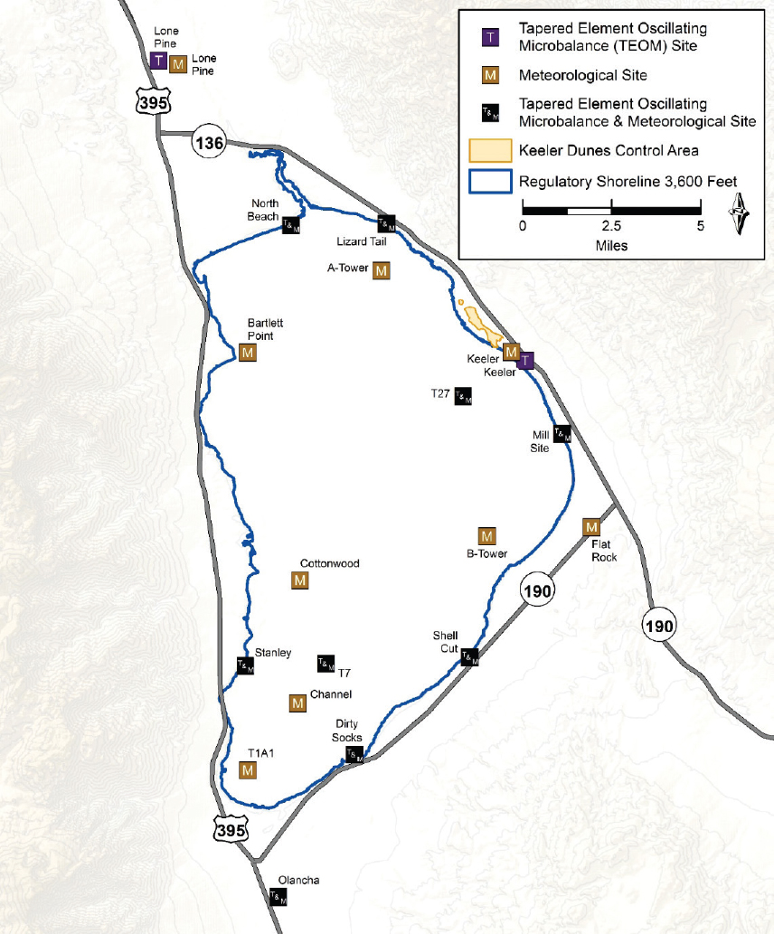
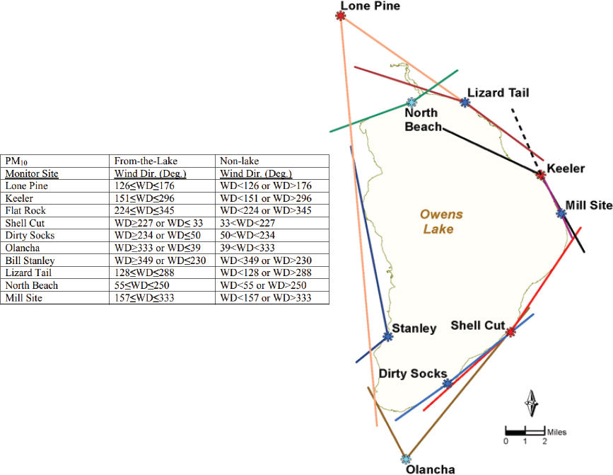
In 1987, EPA determined that the southern Owens Valley area (now referred to as the Owens Valley Planning Area [OVPA]) was in violation of the new NAAQS for PM10. The District monitors PM10 at Keeler, Olancha, Lone Pine, Dirty Socks, Lizard Tail, Shell Cut, Stanley, Mill, and North Beach, both to better characterize the problem, as well as to lay a foundation for developing effective emissions control strategies (see Figure 2-2). These PM10 monitoring sites are all located in areas surrounding the lakebed, both very near the regulatory shoreline and elsewhere in the Owens Valley (e.g., Lone Pine, approximately 3 miles away). On-lake special purpose PM10 monitors are used to determine compliance with required performance criteria. Monitoring is also used to evaluate compliance with the California air quality standards, which are more focused on locations that present exposures to populations.
The compliance monitoring for the NAAQS for PM10 is conducted using Tapered Element Oscillating Microbalance (TEOM) instruments. TEOMs are Federal Equivalent Method (FEM)1 monitors that provide semi-continuous data. Typically reported for compliance purposes on a 24-hour average basis, they can provide data at much shorter time resolutions (minute-level), although shorter averaging times lead to increased uncertainty. At Owens Lake, hourly TEOM PM10 data are reported to EPA. In addition, the Keeler monitoring site has two PM10 Partisol samplers (filter-based, Federal Reference Method [FRM] for sampling the ambient air and analyzing for an air pollutant), as well as a TEOM and Partisols for PM2.5 (particles 2.5 µm or smaller in aerodynamic diameter).2 Filter-based monitoring is typically conducted for 24-hour periods (midnight to midnight), but not necessarily daily. One advantage of filter-based monitoring is that the filters can also be used to conduct speciation (chemical) analysis, and hence provide critical information for source identification, although this use has not been a focus to date. A main disadvantage of using 24-hour filter sampling is that dust events are typically short term (<24 hours), so a 24-hour sample would not fully capture the magnitude of the event, or the relationship to the direction or speed of the wind.
Sensors located next to the PM10 monitors measure wind speed and direction; the resulting information could be used to estimate the direction of the PM10 sources relative to the
___________________
1 A method for measuring the concentration of an air pollutant in the ambient air that has been designated as an equivalent method in accordance with 40 CFR 53.
2 Air quality data statistics for PM10, PM2.5, and other pollutants throughout the state of California are available at: https://www.arb.ca.gov/adam/trends/trends1.php (accessed January 28, 2020).
SOURCE: GBUAPCD, 2016a.
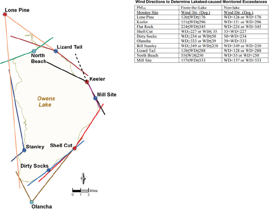
NOTE: Wind directions from the lake toward a PM10 monitor are illustrated by two straight lines extending from a PM10 monitor site to the points on the regulatory shoreline that maximize the angle between the two straight lines in the direction of the lakebed. Wind directions in the table are degrees from the north.
SOURCE: Logan, 2019a.
monitor, as well as provide information for quantifying PM10 emissions. Figure 2-3 illustrates an assessment of wind directions at PM10 monitoring sites to determine whether the origin of the observed PM10 is predominantly from on-lake or off-lake sources. Additional meteorological sites support application of the Owens Lake Dust Identification Model (“Dust ID Model”), which is a tool for identifying dust control areas on the lakebed (GBUAPCD, 2016a).
In addition to the PM10 monitors, the Great Basin Unified Air Pollution Control District in California (District) monitors PM2.5 at the Keeler site (using PM2.5 TEOM and PM2.5 Partisol monitors). Additional PM monitoring is conducted at Federal Class I IMPROVE sites in the area (near Bishop, California), focusing on particles that contribute to haze formation and thereby reduce atmospheric visibility. Those sites include monitors that allow for
speciation of PM2.5 components, which can help inform air quality planners on the transport of PM and, to a degree, relative strengths of emission sources.
TRENDS IN AIR QUALITY MONITORING DATA
Extensive data collection has occurred at various sites in the lake areas, with the key objective to monitor exceedances of NAAQS PM10 levels. Monitoring data show the number of exceedances has steadily decreased since 2000 (see Table 2-1) because of implementation
TABLE 2-1 Exceedances of the PM10 NAAQS at Monitors around Owens Lake from 2000 to 2019
| Year | Area Covered by DCMs (% of lakebed) | Average Exceedance (µg/m3) | Maximum Exceedance (µg/m3) | Exceedance Day Counta |
|---|---|---|---|---|
| 2000 | 0 | 1,087 | 10,840 | 37 |
| 2001 | 10.85 | 1,413 | 20,750 | 46 |
| 2002 | 12.53 | 800 | 7,915 | 49 |
| 2003 | 17.71 | 1,115 | 16,619 | 37 |
| 2004 | 17.71 | 808 | 5,225 | 35 |
| 2005 | 21.41 | 627 | 3,988 | 28 |
| 2006 | 27.37 | 940 | 8,299 | 33 |
| 2007 | 27.37 | 272 | 727 | 14 |
| 2008 | 27.37 | 319 | 814 | 15 |
| 2009 | 27.37 | 339 | 1,506 | 19 |
| 2010 | 36.63 | 603 | 4,570 | 29 |
| 2011 | 36.63 | 641 | 13,380 | 24 |
| 2012 | 38.45 | 495 | 3,916 | 23 |
| 2013 | 38.45 | 283 | 529 | 13 |
| 2014 | 38.45 | 360 | 1,015 | 10 |
| 2015 | 40.75 | 337 | 1,487 | 14 |
| 2016 | 40.75 | 249 | 530 | 16 |
| 2017 | 42.75 | 411 | 2,164 | 17 |
| 2018 | 42.75 | 241 | 728 | 8 |
| 2019b | 42.75 | 280 | 451 | 4 |
a Exceedance Day Count is the number of distinct days during which any PM10 monitor in the Owens Lake area experiences an exceedance of the 24-hour NAAQS for PM10.
b Partial year January to June 2019.
SOURCE: Holder, 2019a; Logan, 2019c.
of DCMs over greater spatial areas with time (Figure 1-3). The maximum 24-hr average PM10 concentration decreased from 20,750 micrograms per cubic meter (µg/m3) in 2001 to 728 µg/m3 in 2018. The total number of exceedance days has decreased from 49 days in 2002 to 8 in 2018. The average exceedance PM10 concentration has also decreased from more than 1,000 µg/m3 in 2000 to fewer than 241 µg/m3 in 2018. Although the DCMs have been effective, certain locations continue to experience exceedances. Thus, further effort is required to bring the region into compliance with the NAAQS for PM10.
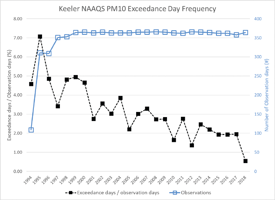
Figure 2-4 shows the variation of exceedances per year at Keeler. Similar to Table 2-1, this figure illustrates improvement over the years, although there have been large year-to-year fluctuations. The fluctuations are likely related to the variation in meteorological conditions that drive emissions, and in the erodibility of the lake surface and off-lake areas. Careful study of the drivers of variability will be critical to management of PM10 control practices in the future.
DATA SOURCE: Logan, 2019c.
NOTE: PM10 means correspond to values in the 2 m/s interval surrounding each point in the plot. Error bars show the standard error of the mean calculated as (2 × standard deviation)/√(number of data points)
DATA SOURCE: Logan, 2019c.
Figure 2-5 illustrates how mean hourly PM10 varies with wind speed for two different years and two sites (Dirty Socks and Keeler), and thereby the linkage of high winds to PM10 concentrations. Both sites reported the expected increase in concentrations with wind speed. However, the patterns of decrease differed between the sites: At Dirty Socks, greater reductions in PM10 concentrations occurred from 2000 to 2017 at increased wind speed, while at Keeler those reductions varied less with wind speed. An understanding of the processes that govern this behavior—informed by more sampling with distributed sensors (Li et al., 2019) and better modeling approaches (discussed later)—will support formulation of strategies to attain the NAAQS.
Although the number of exceedances has clearly decreased over the past two decades, attainment of the NAAQS and the California standards has not yet occurred. Further, the exceedances often result in high PM10 concentrations. For the past 3 years, the maximum
PM10 concentrations are from 3 to more than 10 times the level of the NAAQS, suggesting that considerable emissions reductions are still required.
PM10 EMISSIONS ESTIMATION
As part of its efforts to identify dust sources at Owens Lake that can cause or contribute to exceedances of the NAAQS for PM10, the District uses sand flux measurements to estimate PM10 emissions from the lakebed and off-lake. Sand flux (more generally referred to as horizontal sediment transport) is a measurement of the mass of windblown sand-sized particles moving above the surface per unit time. Estimation of PM10 emissions based on surrogate sand flux measurements involves the use of a semi-empirical relationship that relies on the horizontal movement of particles, whose sizes include diameters greater than 10 µm.
The link between saltation and the emission of fugitive dust containing PM10 may be approximated by
| Fa ∼Kq | (Equation 2-1) |
Where:
Fa is the PM10 emission rate in g/cm2 · s,
K (also known as the K-factor) is a dimensionless constant dependent on surface physical and chemical characteristics, and
q is the horizontal sand flux measured in g/cm2 · s (Gillette et al., 2004; Ono et al., 2011).
Sand flux is measured at Owens Lake using a combination of collocated devices to measure hourly sand flux rates (see Figure 2-6). The instruments are positioned with their sensors or inlets 15 cm (5.9 inches) above the surface. Cox Sand Catchers are passive collection instruments that capture windblown, sand-sized particles (see Figure 2-7) and provide a mass collection amount for a certain sampling period (usually about 1 to 3 months). As battery-powered, sand motion detectors, the Sensit device time-resolves the collected mass to estimate hourly sand flux rates (see Figure 2-7). This device measures the particle counts of sand-sized particles as they saltate, or bounce, across the surface.3
Sand flux monitors at about 200 locations are used to estimate dust emissions and thus source emission rates from the lakebed (see Figure 2-8). There is a new effort to leverage the growing capabilities of inexpensive PM sensors on the lake, but this effort is limited in the number of instruments, their spatial distribution, and the duration of the effort.
___________________
3 For additional information on sand flux measurement methods at Owens Lake, see GBUAPCD (2013c, Attachment C).
SOURCE: EPA, 2019b.
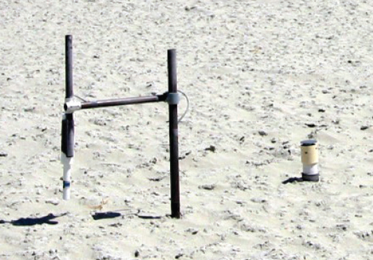
NOTE: The Sensit is a battery-powered motion detector used to count sand-sized particles per unit time that saltate (bounce) across the surface. The Cox Sand Catcher is a passive device used to capture samples of windblown, sand-sized particles of dust at a specific height above the surface.
SOURCE: Richmond, 2019.
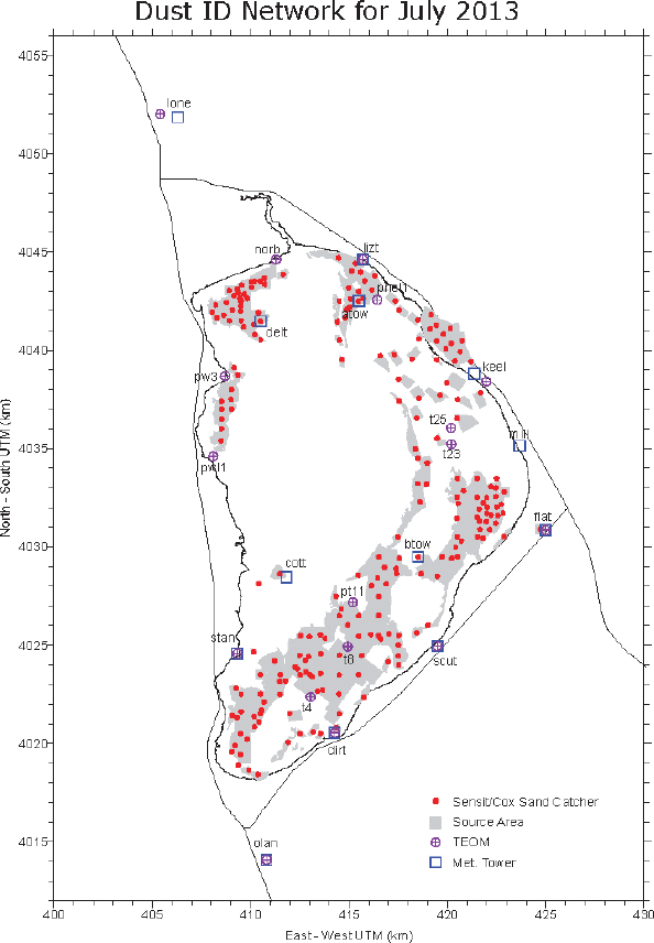
SOURCE: Richmond, 2019.
Use of measured horizontal sand flux to estimate PM10 emissions leads to uncertainty because of the spatial and temporal variability in surface conditions, which are not well represented by a constant K factor (Klose et al., 2019; Kok et al., 2014). The approach to estimating emissions is useful if the K factor does not vary significantly with the surface condition and the wind speed. However, Gillette et al. (2004) indicate that the K factor varies by as much as an order of magnitude, for the same surface type because of variations in surface condition and wind speed, and can vary by many orders of magnitude among surface types.
Uncertainty in the measurement of the sand flux, q, is also large. The Cox Sand Catcher, as used at Owens Lake, (Ono et al., 2003) is a method used for the measurement of sand flux,
with lower efficiency than the samplers used by Gillette et al. (1997). The operating principle also indicates that larger particles may be preferentially trapped (Goosens et al., 2000). Although horizontal sand flux provides useful information on the susceptibility of a surface to wind induced emissions, it does not provide accurate quantitation of PM10 emissions. The substantial uncertainty in the use of proxy measures, such as horizontal sand flux, to estimate PM10 emissions, suggests additional methods be investigated to quantify PM10 emission from individual dust control areas.
There are several portable, real-time instruments for monitoring airborne PM, and recent advances have led to the development of low-cost and yet accurate sensors for real-time measurement of both PM2.5 and PM10 (Bulot et al., 2019; Carvlin et al., 2017; Chung et al., 2001; Johnson et al., 2016; Li et al., 2019; Manikonda et al. 2016). The networking of real-time, low-cost PM10 monitoring devices with existing PM10 monitors on Owens Lake could potentially enable more accurate and precise PM10 measurements, made upwind and downwind of dust control areas, with enhanced spatial and temporal resolution. A network of PM10 sensors along the edges of contiguous dust control areas would allow for better quantification of mean PM10 emission rates and DCM control effectiveness, for example, by using differencing and other inverse modeling techniques. Further, time series of PM10 measurements collected under varying surface and meteorological conditions will enhance knowledge of how those conditions affect PM10 emissions and better inform management decisions.
The South Coast Air Quality Management District of California provides the results of performance assessments of low-cost sensors under field and laboratory conditions (SCAQMD, 2019). Under field test conditions (that did not include testing at Owens Lake), side-by-side comparisons of PM10 sensors with FRM/FEM instruments yielded R2 results ranging from less than 0.25 to 0.66-0.70. The values on the high end of the range are promising because they indicate reasonable agreement between the sensor readings and the FRM/FEM readings.
Given the varied performance of the current generation of low-cost PM10 sensors, it is important to calibrate and test all devices for representative operation under the field conditions encountered on and around the Owens Lake bed. Testing should include
- Multiple types of sensors and potential sampling strategies;
- Sites on the lakebed with different soil textures and during different seasons; and
- Proximity to a meteorological site to obtain observations (e.g., humidity and radiation loading) for characterizing local environmental conditions.
In addition, there should be a transition period during which the deployment of a network of PM10 sensors overlaps with the use of the current network of Sensits and Cox Sand Catchers to determine relationships between the historic sand flux measurements and more directly determined PM10 emissions.
APPORTIONING ON-LAKE AND OFF-LAKE SOURCES OF PM10 EMISSIONS
According to the District, the primary sources of windblown dust in the OVPA include the Owens Lake bed, Keeler Dunes, Olancha Dunes, and other areas close to the regulatory shoreline. Other sources include small mining facilities, areas near the communities of Lone Pine and Independence, intermittent sources near the lakebed caused by flash flood deposits, and regional-scale weather events. Based on an assessment of monitoring and modeling data, the District determined that emissions from off-lake sources more than 2 kilometers away from the lakebed do not have an impact on achieving attainment of the NAAQS (GBUAPCD, 2016).
Historically, the Owens Lake bed has been the major source of windblown dust in the OVPA. However, since the implementation of DCMs nearly 20 years ago, emissions from the lakebed have been decreasing. According to the District, the Keeler Dunes, Olancha Dunes, and other sources of windblown dust near the shoreline now compose a larger fraction of airborne PM10 on days exceeding the NAAQS. Off-lake PM10 emissions continue to pose the largest challenge for demonstrating attainment of PM10 air quality standards within the OVPA (GBUAPCD, 2018).
The role of off-lake sources is illustrated by PM10-Wind velocity plots, such as that shown in Figure 2-9 for the Dirty Socks monitor located at the southern edge of the lake. The plots in the figure show the direction from which the wind is blowing, wind speed, and resulting PM10 concentrations. The plots also show that the source regions for Dirty Socks in 2002 were located in the quadrants to the west and north and that hourly concentrations greater than 500 µg/m3 occurred primarily when the wind speeds were greater than 10 m/s (22.4 mph). These observations highlight the dominant role of PM10 sources on the lake. With emission controls established by 2017, Figure 2-9 illustrates that, based on Dirty Socks monitoring data, the dominant source regions are primarily in the south with winds greater than 10 m/s leading to high concentrations, suggesting the importance of off-lake sources.
These results, although based on limited data, suggest that control strategies will need to place greater emphasis on off-lake sources to achieve attainment of NAAQS for PM10. To bring the region into compliance, the impact of specific source regions must be firmly understood. More thorough analyses of wind speed and wind direction, coupled with dispersion models, would help to identify regions (sources) and inform the development of effective control strategies. If feasible, back trajectories could help to identify the specific source areas and emissions of PM10 during exceedances, and better determine whether the event is primarily driven by on-lake or off-lake emissions.
STATE IMPLEMENTATION PLAN DEVELOPMENT AND AIR QUALITY MODELING
Because the OVPA is a nonattainment area, California is required to develop a SIP that lays out a path for attainment of the NAAQS. In this case, California has delegated that task to the District. The SIP developed by the District must be approved by both California
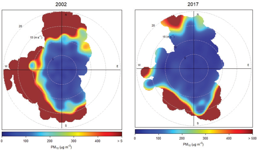
NOTES: Source regions are identified by compass directions, and the associated wind speeds in m s−1 correspond to the radii of the circles. The color indicates PM10 concentrations in µg m−3 (µg/m3). Concentration distributions vary with wind direction, and concentration magnitudes increase rapidly with wind speed. The distribution of PM10 concentrations across the color scale can affect the transition from one color to another. Sharper transitions occur when there are larger gaps between concentration values. Looking at the 2017 plot, the blue area, representing lower PM10 concentrations, occurs at lower wind velocities (i.e., nearer the center of the circle). Much of the high PM10 concentrations (brown) occur at higher wind velocities (15-20 m/s) when the wind is coming from the south, north, or northwest, with a smaller fraction coming from almost due west. Those results suggest the importance of off-lake sources.
DATA SOURCE: Logan, 2019c.
and EPA. Developed in 1998, the first PM10 SIP for the Owens Lake area proposed attainment by 2006, which was not achieved. The continued nonattainment in the region has led to additional SIPs and SIP revisions in 2003, 2008, 2011, 2013, and 2016.
Air quality models play a central role in determining the amount of PM10 emission reductions that will be needed to bring about compliance with the NAAQS. The 2016 SIP approved by EPA concluded that “Air quality modeling has shown that this [proposed control] strategy can reduce PM10 impacts at sites above the regulatory lake shore to below the federal 24-hr PM10 standard by the end of 2017” (GBUAPCD, 2016a, p. S-15). That reduction was not achieved.
A major feature of a SIP is demonstration of attainment that involves air quality modeling. The type of air quality model applied depends on the pollutant, and EPA provides guidance for
model choices (EPA, 1996). Typically, a specific model is applied to prove its ability to reproduce historical airborne pollutant concentrations, and then alternative emissions levels are simulated to reflect the results of controls being applied to sources or source regions in the modeling domain. For the Owens Valley SIPs, the modeling approach has evolved, and the 2016 SIP applied a hybrid approach based on the CALPUFF/CALMET (version 6.4) modeling system (Allwine et al., 1998; GBUAPCD, 2016a; Scire et al., 1990). CALPUFF is a multilayer dispersion model without chemical reactions, which is appropriate for modeling PM10, particularly over the time and distance scales involved here. As noted by EPA (2018), CALPUFF was de-listed as an EPA preferred model in its 2017 guidelines on air quality models for regulatory application, because the model was considered by the agency to no longer be needed. Although usually used for longer-range transport (more than 50 km [31 miles]), it can be used for shorter-range dispersion modeling when the three-dimensional (3-D) features of the winds are viewed as important. Otherwise, steady-state dispersion models (e.g., AERMOD; Cimorelli et al., 2005) are often used. Winds in the Owens Lake area can be complex, varying rapidly in space and time, because of the topography (e.g., the Sierra and other surrounding mountains). As a hybrid application, CALPUFF can use observations to estimate the impact of off-lake sources. CALPUFF was also updated to allow for more finely resolved emissions inputs to reflect the rapidly changing emissions estimated from sand flux measurements.
Critical inputs into the air quality modeling include the meteorology and the emission flux. Meteorological characteristics are monitored throughout the lakebed and surrounding areas (e.g., to obtain upper air variables) and are processed using CALMET, which is a computation model based on physical processes (Scire et al., 2000). For emissions modeling in this case, the approach is multistep, first estimating emissions and then adjusting the emissions to improve model performance. As discussed previously in this chapter, dust emissions from the lakebed are estimated using a relationship proposed by Gillette et al. (1997) involving an empirical K factor that relates sand flux to PM10 emissions (Ono et al., 2011). K factors are first estimated based on time period and surface type and, if present, DCM. After CALPUFF is run, its results are compared to the observations, and the K factors are adjusted to obtain better agreement.4 This need for adjustment suggests uncertainty in the K factors. Given the linearity of the system, the uncertainties in the K factors will propagate to uncertainties in the simulated concentrations. The accuracy of air quality models would benefit from direct quantification of DCM effectiveness with far more certainty than is currently achieved using horizontal sand flux as a surrogate for PM10 emissions. The importance of accurate estimates of a DCM’s effectiveness in controlling PM10, and improved estimates of associated uncertainties, increases as airborne PM10 concentrations approach the allowable level of the air quality standards.
___________________
4 Further details of how the K factors are derived are provided in the 2016 SIP (including Appendix VII-1).
In this type of application, the credibility of the air quality model must be established; in this case by showing that the model adequately captures historic observations, with a specific focus on conditions leading to exceedances. Then the model is run to determine the level of emission control required to attain the NAAQS for PM10. The model is assumed to be a virtual surrogate for the real system. The model allows for numerical experiments to be conducted that would be impractical to be carried out in the real system.
The modeling approach presented to the panel can be improved significantly. For example, Richmond (2019) indicated that the model often does not explain the temporal variability of the observations. Furthermore, the model did not estimate 40 of the 194 exceedances of the NAAQS observed during July 2009 to June 2014. The evaluation results of the model presented in Richmond (2019) focused on days for which the measured average concentrations were greater than 150 µg/m3, based on the assumption that good performance of a dispersion model for predicting high concentration days lends credibility to the model’s ability to predict NAAQS attainment. However, it is also necessary to assess the model’s performance when it estimates concentrations greater than 150 µg/m3 but the observed concentrations are lower than the NAAQS level. Such an assessment is important because attainment demonstration requires estimating PM10 concentrations that are less than the NAAQS level or when observations are not available.
Model performance and hence the reliability of future projections of air quality can be improved by paying more attention to the processes that dominate emissions and dispersion during high winds, when the highest PM10 concentrations occur (see for example, Shiyuan et al. 2008). The modeling of vertical dispersion can be improved within the framework of CALPUFF by using dispersion coefficients based on internally calculated micrometeorological variables rather than the Pasquill-Gifford curves formulated more than 60 years ago. Better still, dispersion curves that are specifically formulated for near surface releases and reflect the current understanding of dispersion and micrometeorology (Cimorelli et al., 2005) could be used. This option requires expressing model inputs in terms of variables, such as friction velocity, which controls dispersion as well as emissions. Those variables can be measured using a 3-D sonic anemometer or estimated with the CALMET processor. Efforts to improve the dispersion model and its inputs to reflect the state of the art and then to evaluate against observations would better inform decision making on emission control related to NAAQS attainment. It is also important to identify, and to the extent feasible quantify, the sources of uncertainty in the model. See NRC (2007) for a discussion of quantifying and communicating uncertainties.
CONCLUSIONS AND RECOMMENDATIONS
This section presents the panel’s key conclusions and recommendations concerning progress in managing airborne PM10, quantifying PM10 emissions, and air quality modeling.
Progress in Managing Airborne PM10
Conclusion: Because of the efforts of the District and LADWP, airborne PM10 concentrations at monitoring locations in the OVPA have decreased significantly since the implementation of DCMs on Owens Lake.
Quantifying PM10 Emissions
Conclusion: Estimates of reductions in PM10 emissions are associated with a high degree of uncertainty because they have relied primarily on measurements of sand flux. The size-dependent performance and other measures of sampling efficiency are not available for the Sensits and Cox Sand Catchers, which are used to measure sand flux. The K-factor values imputed by the observations are highly variable, greatly impacting estimated current and future emissions.
Conclusion: Increased use of low-cost sensors and other advanced PM monitoring techniques would help to characterize the location and magnitudes of the high source regions, further helping to quantify the control efficiencies of the DCMs being utilized on and around the lakebed.
Recommendation: The District and LADWP should develop and apply additional methods to quantify, with uncertainty estimates, PM10 emissions from individual dust control areas, based on direct measurements of airborne PM10 concentrations.
All devices should be calibrated and tested for representative operation under the field conditions encountered on and around the Owens Lake bed. Testing should include
- Multiple types of sensors and potential sampling strategies;
- Sites on the lakebed with different soil textures and during different seasons; and
- Proximity to a meteorological site to obtain observations (e.g., humidity and radiation loading) for characterizing local environmental conditions.
In addition, there should be a transition period during which the deployment of a network of PM10 sensors overlaps with the use of the current network of Sensits and Cox Sand Catchers to determine relationships between the historic sand flux measurements and more directly determined PM10 emissions.
Air Quality Modeling
Conclusion: The panel recognizes the complexity of the processes that govern PM10 emissions from the Owens Lake area and the subsequent transport and dispersion of
those emissions. However, the modeling approach used to demonstrate attainment of the NAAQS for PM10 does not use state-of-the-art dispersion formulations.
Conclusion: The modeling conducted as part of the 2016 SIP would be improved with increased evaluation and uncertainty analysis, as suggested by the National Research Council report Models in Environmental Regulatory Decision Making (NRC, 2007).
Conclusion: Given the continued nonattainment in the OVPA, additional analysis and documentation of the failure of past emission control strategies are needed.
Recommendation: Approaches to air quality modeling to demonstrate attainment of the NAAQS for PM10 should incorporate the current understanding of micrometeorology and dispersion, especially during periods of high winds. Particular attention should be given to characterizing the conditions leading to exceedances, and identifying major source locations both on- and off-lake. Furthermore, the uncertainty associated with modeling those processes should be factored into plans to attain the NAAQS.


