
4
Current Conditions, Trends, and Future Stressors
Managing the complex, combined influence of watershed characteristics and land use on the quantity, quality and timing of streamflow is a central focus of the Watershed Protection Program. This chapter includes a brief description of the hydrological regime of the Catskills region, an overview of land cover and land use trends in the watersheds, a summary of the water quality concerns in the New York City (NYC) drinking water supply system, and a review of some of the ways that climate change may change these stressors in the future.
The west-of-Hudson (WOH) watersheds encompass a humid, temperate, mountainous landscape with a large proportion of forest land (72 to 93 percent across the six reservoir watersheds) and smaller proportions of other land uses, primarily agriculture and developed areas. All land covers and land uses have the potential to generate pollutants that flow to the NYC water supply reservoirs. Hence, the product of streamflow discharge and pollutant concentration (loading) defines the operational challenges faced by the NYC Department of Environmental Protection (NYC DEP) and enumerated in the filtration avoidance determination (FAD) and other applicable laws and regulations.
The water supply system was designed, and is managed and operated, to avoid or minimize fluctuations in drinking water quality. The resilience of the watersheds, water supply infrastructure, and operational skills of NYC DEP staff have been repeatedly tested by wet and dry years, as well as shorter periods of atypical weather conditions. These challenges will continue as prospective growth in the number of water consumers in NYC and surrounding communities place new demands on the system. In addition, the “warmer, wetter” conditions forecast by global circulation models and evident in statistical analyses of long-term streamflow records (1951-2017; NASEM, 2018) are likely to influence water quality conditions in the reservoirs and require new operational adaptations and refinements.
CLIMATE AND HYDROLOGIC REGIME
The mountainous terrain and strongly seasonal climate of the Catskill region directly influence temporal patterns of streamflow. Orographic precipitation (induced by lifting and cooling) is a common occurrence as air masses flow up and over the mountains (cooling by ~6 °C per 1,000 meters). Substantial differences in air temperature between mountaintop, mid-slope, and valley bottom sites during the fall and spring can lead to snow at the top, mixed precipitation in the middle, and rain at the bottom of this elevational transect during precipitation events. In addition, total annual precipitation is strongly related to elevation (e.g., median year totals of ~1,100 to 1,200 mm in the valleys and ~1,500 mm or more on the mountaintops, with a larger proportion falling as snow).
Temporal patterns of snow accumulation and melt were, with some interannual variability, reasonably consistent and predictable during the 19th and 20th centuries. The snowpack typically formed in late November
or early December on the mountaintops, extended across the region in December and January, increased in depth during the cold winter months, then melted in March, April or early May, often producing the annual peak discharge for the water year. More recently, the temporal patterns of snow accumulation and melt have become more erratic, with varying combinations of rain, snow, rain-on-snow and snowmelt events occurring from the late fall to the early spring.
The typical sequence of hydrologic seasons during the water year1 (October 1 to September 30) in the Catskills (and other parts of the northeastern United States) includes:
- Fall recharge of soil water content with progressively larger increases in streamflow during October and November;
- Snow accumulation during December, January and February;
- Mixed precipitation and snowmelt in March or early April with increases in streamflow corresponding to the size and melt rate of the snowpack;
- Spring transition as the forest vegetation comes out of dormancy (late April through mid-May) and active uptake of soil water begins and streamflow decreases;
- The growing season (mid-May through late August) when evapotranspiration reaches an annual maximum and, in consequence, streamflow decreases to annual minimum values; and
- The fall transition with leaf-fall and dormancy (September and the beginning of the next water year).
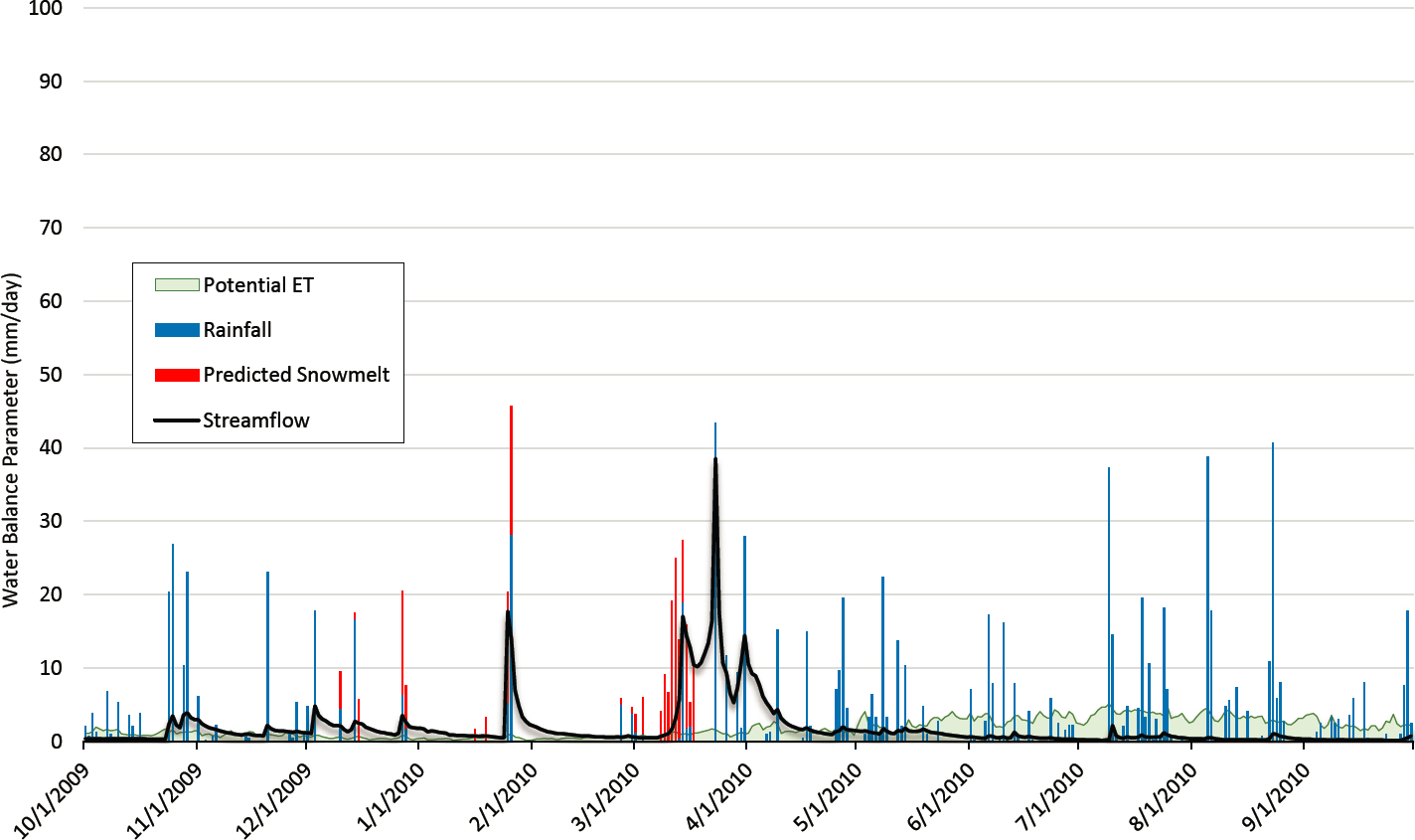
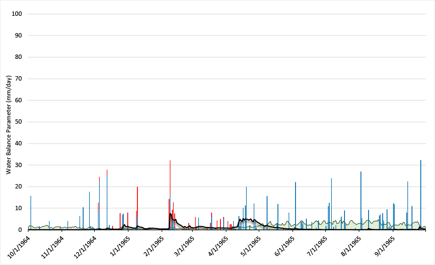
The mean water year (2010) presented later in this section is a good example of the sequence of hydrologic seasons summarized above. In contrast, the driest year of record (1965) shows the cumulative effect of reducing precipitation by one-third, while evapotranspiration remains about the same. The wettest year of record (2011) shows the cumulative effect of exceptional precipitation events.
Regional weather patterns in the Catskills are influenced by air masses from all four cardinal directions: continental, continental polar, maritime tropical, and maritime polar throughout the year. Hurricanes, tropical storms, tornadoes, and severe convective storms may occur throughout the late spring, summer, and fall. The most recent extreme events were Tropical Storm Irene (August 2011), Tropical Storm Lee (September 2011), and Hurricane Sandy (October 2012).
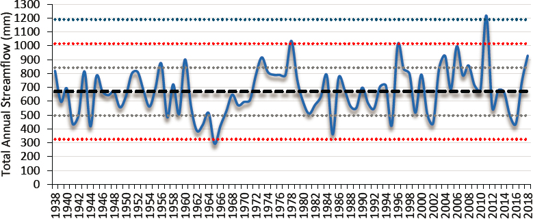
Water supply managers and watershed residents have a well-developed sense of the wide range of variation in precipitation and streamflow in the Catskills and the associated challenges for the operation of New York’s water supply system. As shown in Figure 4-1, the total annual water yield for the East Branch of the Delaware River in Margaretville varies widely around a mean of 670 mm, considering 80 years of data from 1938 to 2018. The NYC DEP water supply operations center (and related programs and teams) must continually assess and compensate for changes in quantity, quality, and timing of inflow to the reservoir system to ensure a uniform flow of high-quality water to consumers.
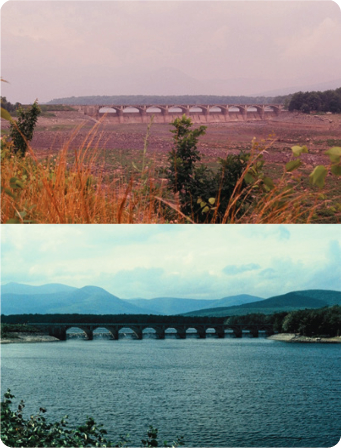
The 1960s drought has been the most severe test of the water supply system (on the dry end of the spectrum) to date. Ten consecutive years of below-average streamflow (1961-1971, with the most extreme conditions occurring in 1962 [390 mm] and 1965 [290 mm]), reduced water yield and reservoir storage to unprecedented levels. Other dry years (1985 [360 mm; Figure 4-2], 1995, 2012, and 2016) have been challenging, but their limited duration, coupled with decreases in mean daily water use,2 have not pushed the system to the hydrological and operational extremes experienced in the 1960s. Nevertheless, dry years require careful stewardship, proactive water conservation in New York City and other communities, and exacting operational control. As soon as a pattern of dry conditions (and a challenging long-range forecast) becomes evident, guarding against the eventuality of consecutive dry years is the most prudent management paradigm. The long-term staff experience, the Operations Support Tool, advances in weather forecasting technologies, real-time monitoring, and major advances in computing capabilities have substantially increased the NYC DEP’s ability to proactively respond to drought emergencies (NASEM, 2018).
___________________
1 Hydrologists use the water balance (Precipitation – Evapotranspiration – Water yield ±∆ Storage = 0) for the “water year” (when the net change in storage for Day 1 versus Day 365 is negligibly small) to consistently estimate the size of the other three terms. At the watershed scale, the storage term includes soil water content, wetland and shallow aquifer water levels, and baseflow in the stream network. In the northeastern United States, the quantity of water in storage is usually comparable when the period of analysis begins on October 1 and ends on September 30.
2 From 1,300 MGD in 1985 to 1,000 MGD in 2016 (Figure 3-5), with per capita water consumption decreasing from 180 GPD in 1985 to 120 GPD during 2008 to the present (latter data courtesy of NYC DEP).
Periods of unusually high streamflow present another set of challenges to water supply managers. Very large rainfall, snowmelt, and/or rain-on-snow events can transport large quantities of sediment, nutrients and other contaminants to the reservoir system. As noted earlier, the most recent and extreme examples were Tropical Storms Irene and Lee (August and September 2011, respectively). Analyses of long-term weather station data show that other very high streamflow years (e.g., 1978, 1996, and 2006) were caused by a combination of: (1) very large, high-intensity dormant-season rain events, (2) exceptional snow accumulation (e.g., 450 mm snow water equivalent in 1978), and/or (3) delayed, then rapid snowmelt in late April or early May. Simply put, when total annual rain and snow water equivalent approaches or exceeds 2,000 mm, high water yield and potentially damaging streamflow discharge(s) are inevitable.
Focusing on the challenges associated with very dry and very wet years does not diminish the relatively frequent operational challenges associated with somewhat unusual meteorological events in any given year. For example, several weeks with little or no rainfall can rapidly diminish streamflow and adversely influence water quality (e.g., increased water temperature and BOD). In contrast, a series of closely spaced rain events can rapidly (and progressively) increase streamflow with associated changes in water quality (e.g., increased turbidity). The dynamic nature of Catskill Mountain watersheds underscores the importance of the NYC DEP’s emphasis on preparedness, advanced training, vigilance, and adaptability for the Water Supply Operations Center and all other parts of the organization.
The cause-effect interrelationships of rain, snowmelt, evapotranspiration, and streamflow, and the influence of seasonal changes in water storage (in the snowpack, soil, shallow unconfined aquifers, and streams) are evident in daily data for a mean water year (2010) and the driest (1965) and wettest (2011) water years of record (Table 4-1 and Figures 4-3, 4-4, and 4-5). All three figures are presented with a daily time step on the x-axis and the same y-axis dimension (100 mm) to facilitate direct comparison.
As can be seen in Figures 4-3 to 4-5, the annual totals of streamflow (water yield) are clearly related to total precipitation. In addition, the timing of streamflow is influenced directly by rain events and temporal patterns of snow accumulation and melt. In most years, the snowpack forms a layered composite of the precipitation events over many months before melting en masse in just a few weeks during March or April. During most years, the dormant season (October through April) typically accounts for about three-fourths of annual water yield. A few large rain events during the growing season (mid-May through early September) typically generate the remaining approximately one-fourth of annual water yield.
Growing season streamflow is also strongly influenced by evapotranspiration (interception of water by the plant canopy, transpiration [water use] by plants, and evaporation of water from soils, the snowpack, wetlands, streams, ponds, lakes and reservoirs). Potential evapotranspiration (PET) is an estimate of the upper limit of atmospheric demand, under the prevailing conditions for any given day, when the supply of water is not limited. In Figures 4-3 to 4-5, PET was calculated with the Hamon (1961) equation and day length from the US Naval Observatory ephemeris. Actual evapotranspiration (AET) is difficult to estimate on a daily basis without
TABLE 4-1 Summary of water balance parameters for the three water years, East Branch of the Delaware River at Margaretville, New York (USGS Gaging Station 00141350), 1937-2018, and Delhi 2 SW meteorological station (NOAA Meteorological Station USC00302036)
| Water Year | Rain (mm) | Snowa (mm) | Potential ETb (mm) | Streamflowc (mm) |
|---|---|---|---|---|
| 1965 (Driest) | 620 | 130 | 620 | 290 |
| 2010 (Mean) | 940 | 190 | 650 | 670 |
| 2011d(Wettest) | 2,020 | 190 | 630 | 1,220 |
a Snow = snow water equivalent (liquid water released by snowmelt).
b Potential ET (evapotranspiration rate when the supply of water is not limited).
c Streamflow = the sum of mean daily discharge (ft3/s), divided by watershed area, then converted to mm/day and summed for the water year.
d The total precipitation estimate for January-September 2011 was derived from observations at the Walton, New York and Slide Mountain, New York stations after observations at the Delhi 2 SW station were discontinued at the end of 2010.
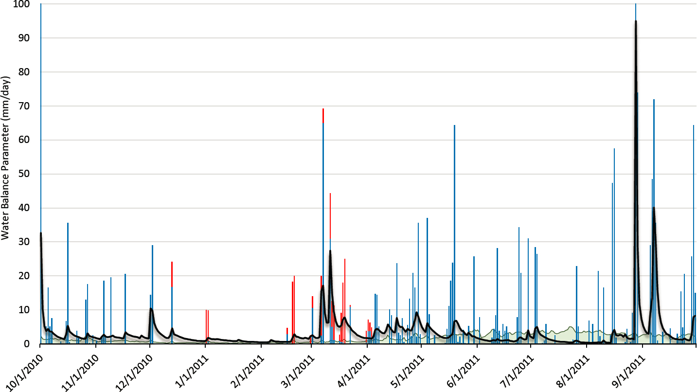
detailed micrometeorological data and accurate measurements of changes in soil water content, depth to the saturated zone, and water levels in wetlands and waterbodies. However, on a water-year basis, when the net change in total storage is negligibly small, AET can be simply and accurately estimated as the difference between total precipitation and total streamflow (e.g., 460 mm for both 1965 and 2010). This estimation method is not viable for the 2011 water year; the 150-mm rain event on October 1, 2010, the unprecedented size of the tropical storms in late August and mid-September 2011, and substantial rainfall during the last three days of the water year, negate the assumption of negligible changes in storage and preclude the estimation of AET as the water balance residual.3
Evapotranspiration varies little from year to year, with its most dominant effect consistently occurring during the growing season, when longer days, warmer temperatures, and transpiration by plants have the combined effect of returning large volumes of water to the atmosphere. Evapotranspiration simultaneously decreases soil water content, the areal extent of the saturated source area, and water levels in wetlands and shallow, unconfined aquifers. This available storage has the direct (often major) effect of reducing streamflow response to rain events during June, July, and August. The paucity of rain and snow during the driest year of record (1965) and dominant effect of evapotranspiration reduced water yield to 40 percent of the long-term mean (290 mm). In contrast, water yield during the wettest year of record (1,220 mm) was nearly double that of the mean year. There were two rain and/or snowmelt events greater than 30 mm in 1965, five in 2010, and 17 in 2011 (seven were >60 mm in 2011).
***
The historical record demonstrates the highly variable nature of climatological and hydrological conditions in the Catskills. The most daunting operational challenges occur at the two extremes of the historical range of variation (i.e., the 1960s drought and tropical storms of 2011). The challenges and uncertainty associated with dry years require (1) early recognition that drought may have begun, (2) careful stewardship of supplies, and (3) substantial, simultaneous reductions in demand until storage in the system has returned to long-term average conditions. In contrast to prolonged drought periods, the sudden, often drastic, changes associated with extreme events (e.g., hurricanes, tropical storms, severe convective storms, rain-on-snow events, late-season melting of a deep snowpack, and others) compel NYC DEP staff to react quickly as discharge and pollutant loading changes by orders of magnitude on a time scale of hours or days. After the flood emergency conditions have passed, the lingering effects (e.g., elevated turbidity in key reservoirs) require months of careful management to resolve. Recent analyses of long-term patterns and trends in reference watersheds across the Catskill and Delaware Systems (NASEM, 2018: Appendix A) and in this report presage new operational challenges as the effects of global climate change unfold. That is, the extent to which global climate change effects (1) total precipitation, (2) the proportion and timing of rain and snow events, (3) rainfall intensity and snowmelt rates, (4) snow accumulation and melt, (5) evapotranspiration, and, in consequence, (6) the quantity and timing of streamflow adds another layer of complexity to the historic range of variation in the Catskills. To that end, a rigorous mathematical modeling experiment (“stress test”) undertaken by the NYC DEP at the request of the Committee is described in detail later in this chapter. It convincingly demonstrated the flexible and adaptive nature of both the water supply system and the operations staff and, reassuringly, the capacity to effectively meet the inevitable challenges of the 21st century.
LAND USE AND LAND COVER
Land use and land cover are key drivers of anthropogenic effects on freshwater ecosystems (Gergel et al., 2002). Land cover and use in any watershed influence the hydrologic, biogeochemical, and ecological functions of associated freshwater systems (Johnson et al., 1997; Niyogi et al., 2004; Rabalais et al., 2002; Richards et al., 1996; Sweeney et al., 2004). NRC (2000a) identified the need for a complete inventory of land use and potential pollutant point sources in the WOH watershed. It also emphasized the need for coordination of watershed monitoring and modeling programs to quantify the proportional contributions of the diverse range of land covers and land uses to total pollutant loading of the reservoir system.
___________________
3 AET must, by definition, be less than or equal to PET (Brooks et al., 2013).
Land Cover Change Analysis
The Committee conducted a GIS analysis using the National Land Cover Database (NLCD)4 for the WOH and east-of-Hudson (EOH) watersheds to evaluate cumulative changes in land cover between 2001 and 2016. It found that land cover change across the 1 million-acre WOH watershed was barely detectable during this 15-year period, about 0.034 percent of the total land area (Tables 4-2 and 4-3). Conversion of small areas from farm and forest land to developed and other land covers accounted for 0.05 percent of the watershed area between 2001 and 2016. This rate of land cover change was about one-hundredth of the average rate of change for New York State (4.1 percent) as a whole reported by Homer et al. (2020) in a standardized, comprehensive analysis of the conterminous United States by the U.S. Geological Survey. Land cover change across the 248,000-acre EOH watershed was larger in relative terms, 1.8 percent (Tables 4-4 and 4-5). This change was also attributable to farm and forest conversion to developed land cover types. However, this was still less than half of the statewide average, 4.1 percent, and equivalent to the rates of land use change in Vermont and Maine during the same 15-year period (Homer et al., 2020).
Forest and agricultural land conservation programs and a wide range of socioeconomic and regulatory factors (discussed throughout this report) appear to have minimized land cover change for almost two decades in both watersheds of the NYC water supply. In absolute terms, the rates of land cover change were ~25 acres per year for the 1-million-acre WOH watershed and ~280 acres per year for the 248,000-acre EOH watershed.
The net effect of converting forest or agricultural land to some form of development on streamflow and water quality in adjacent streams, and ultimately on the reservoir system, is dependent on the topography, soil properties, proximity to the stream network, and other site-specific factors. The specific nature and characteristics of the new land use within the relatively broad land cover categories (de la Crétaz and Barten, 2007; NRC, 2008) also influence soil surface conditions, pathways of flow (e.g., overland, through the root zone, and/or deeper groundwater routes), and quantity and mobility of potential pollutants. A primary concern of the Watershed Protection Program is the reduction, whenever and wherever possible, of nonpoint source pollutant loadings. For example, forest land that was a sink for large amounts of nitrogen used by trees during the growing season has the potential to become a source of nitrogen if the site is converted to an overfertilized lawn. Other changes such as surface compaction (leading to overland flow during any rain event that exceeds the infiltration capacity of the soil) can also exacerbate the transport of nonpoint source pollutants to nearby streams. Converting a forest to high-intensity developed use also has the potential to increase stormwater discharges and introduce new forms of water pollution (e.g., hydrocarbons and metals) associated with human activity (de la Crétaz and Barten, 2007).
Classification Accuracy and Scope of Inference
The classification accuracy of the NLCD varies across the 15 land cover types. It is highest for large, homogeneous patches (e.g., extensive forest areas, lakes and reservoirs, cultivated crops) with a uniform spectral reflectance signature. It is lowest for small, heterogeneous patches (e.g., suburban areas with a complex mix of reflecting surfaces, such as rooftops, lawns, driveways, gardens, and shade trees) wherein spectral reflectance values are averaged by the sensor (438 miles above the Earth) across 30-meter pixels in Landsat imagery. The overall accuracy of the land cover classification across the 15-year time series is estimated to be 82-83 percent (with a small standard error of ±0.5 percent) by the Multi-Resolution Land Characteristics Consortium (Homer et al., 2020). However, since the classification errors are randomly distributed and unbiased (i.e., not systematic), the value of the NLCD time series for change detection is higher than the somewhat modest overall accuracy might suggest. Misclassification typically occurs between similar categories (e.g., low-intensity development that is actually medium-intensity development with substantial tree cover).
Classification algorithms include pattern recognition, adjacency tests, and other geospatial data (e.g., National Wetlands Inventory, soil series, and topographic characteristics) to enhance accuracy and consistency across complex landscapes and time series. Hence, the estimates of the relative size of the 15 land cover classes and very high USGS cartographic standards produce accurate estimates of change over time.
___________________
4 See www.mrlc.gov.
TABLE 4-2 Summary of Land Cover in 2001 and 2016 in the West-of-Hudson Watersheds
| Land Cover | 2001 Acres | 2016 Acres | Change (acres) | % of Watersheda |
|---|---|---|---|---|
| 1. Open water | 22,108 | 21,870 | -238b | n/a |
| 2. Developed, open space | ,159 | 36,216 | 57 | 0.006 |
| 3. Developed, low intensity | 3,363 | 3,441 | 78 | 0.008 |
| 4. Developed, medium intensity | 654 | 788 | 134 | 0.014 |
| 5. Developed, high intensity | 209 | 240 | 31 | 0.003 |
| 6. Barren land | 3,124 | 3,134 | 10 | 0.001 |
| 7. Deciduous forest | 568,437 | 561,445 | -6,992 | -0.705 |
| 8. Evergreen forest | 53,642 | 53,258 | -384 | -0.039 |
| 9. Mixed forest | 216,269 | 216,144 | -125 | -0.013 |
| 10. Shrub/scrubc | 1,032 | 6,314 | 5,283 | 0.533 |
| 11. Herbaceousc | 2,363 | 5,728 | 3,365 | 0.339 |
| 12. Hay/pasture | 92,329 | 90,668 | -1,661 | -0.168 |
| 13. Cultivated crops | 1,226 | 1,427 | 201 | 0.020 |
| 14. Woody wetlandsd | 10,916 | 11,008 | 92 | 0.009 |
| 15. Herbaceous wetlandsd | 1,668 | 1,816 | 148 | 0.015 |
| Total | 1,013,498 | 1,013,498 | - | - |
SOURCE: 30-meter resolution National Land Cover Database.
a (Change/Total Land Area) x 100; Total Land Area = 991,390 acres.
b Seasonal differences in water level, flooded area, and exposed shoreline when the 2001 and 2016 satellite images were acquired.
c In contrast to arid and semi-arid areas of the United States, in the humid, temperate northeastern United States, the Herbaceous and Shrub/scrub categories are, in most cases, seedling-stage and sapling-stage forest regeneration, respectively, on fallow or abandoned agricultural fields or forest land where a large proportion of the mature trees (>80 percent) were cut.
d As with open water areas, the classification of wetland types can be influenced by interannual differences in water level and successional processes (e.g., trees and shrubs growing on sites initially classified as herbaceous wetlands).
NOTE: Spatial data are reported at a 1-acre resolution for accounting purposes. The accuracy and precision of satellite images and classification methods varies by land cover type and may, in some cases, be substantially lower (e.g., ±10 to ±100 acres) than one acre. Nevertheless, the Committee adhered to the reporting norms of the Multi-Resolution Land Characteristics Consortium in the peer-reviewed literature (e.g., Homer et al., 2020).
TABLE 4-3 Further Analysis of Cumulative Land Cover Change, 2001-2016, in the West-of-Hudson Watersheds
| Land Cover Classesa | 2001 Acres | 2016 Acres | ∆ Acres | ∆% Watershed |
|---|---|---|---|---|
| Forest (all age and size classes; 6, 7, 8, 9, 10, 11) | 844,866 | 846,024 | 1,157 | 0.12 |
| Hay/pasture (12) | 92,329 | 90,668 | -1,661 | -0.17 |
| Subtotal | -503 | -0.05 | ||
| Developed land (all types; 2, 3, 4, 5) | 40,384 | 40,685 | 301 | 0.03 |
TABLE 4-4 Summary of Land Cover in 2001 and 2016 in the East-of-Hudson (Croton System) Watersheds
| Land Cover | 2001 Acres | 2016 Acres | Change (acres) | % of Watersheda |
|---|---|---|---|---|
| 1. Open water | 15,693 | 15,464 | -228b | n/a |
| 2. Developed, open space | 32,021 | 33,553 | 1,531 | 0.66 |
| 3. Developed, low intensity | 11,135 | 12,367 | 1,232 | 0.53 |
| 4. Developed, medium intensity | 4,845 | 6,034 | 1,188 | 0.51 |
| 5. Developed, high intensity | 1,293 | 1,611 | 319 | 0.14 |
| 6. Barren land | 386 | 342 | -44 | -0.02 |
| 7. Deciduous forest | 143,903 | 139,317 | -4,586 | -1.97 |
| 8. Evergreen forest | 1,528 | 1,482 | -46 | -0.02 |
| 9. Mixed forest | 10,985 | 10,941 | -43 | -0.02 |
| 10. Shrub/scrub | 211 | 437 | 225 | 0.10 |
| 11. Herbaceous | 563 | 2,286 | 1,723 | 0.74 |
| 12. Hay/pasture | 9,224 | 7,959 | -1,265 | -0.54 |
| 13. Cultivated crops | 84 | 50 | -33 | -0.01 |
| 14. Woody wetlandsc | 15,782 | 15,717 | -64 | -0.03 |
| 15. Herbaceous wetlandsc | 240 | 332 | 92 | 0.04 |
| Total | 247,892 | 247,892 | - | - |
SOURCE: 30-meter resolution National Land Cover Database.
a (Change/Total Land Area) x 100; Total Land Area = 232,199 acres.
b Seasonal differences in water level, flooded area, and exposed shoreline when the 2001 and 2016 satellite images were acquired.
c As with open-water areas, the classification of wetland types can be influenced by interannual differences in water level as well as successional processes (e.g., trees and shrubs growing on sites initially classified as herbaceous wetlands).
NOTE: Spatial data are reported at a 1-acre resolution for accounting purposes. The accuracy and precision of satellite images and classification methods varies by land cover type and may, in some cases, be substantially lower (e.g., ±10 to ±100 acres) than one acre. Nevertheless, the Committee adhered to the reporting norms of the Multi-Resolution Land Characteristics Consortium in the peer-reviewed literature (e.g., Homer et al., 2020).
TABLE 4-5 Further Analysis of Cumulative Land Cover Change, 2001-2016, in the East-of-Hudson (Croton System) Watersheds
| Land Cover Classesa | 2001 Acres | 2016 Acres | ∆ Acres | ∆ % Watershed |
|---|---|---|---|---|
| Forest (all age and size classes; 6, 7, 8, 9, 10, 11) | 157,576 | 154,805 | -2,771 | -1.2 |
| Hay/pasture (12) | 9,224 | 7,959 | -1,265 | -0.5 |
| Subtotal | -4,036 | -1.7 | ||
| Developed land (all types; 2, 3, 4, 5) | 49,295 | 53,565 | 4,270 | 1.8 |
Temporal Changes within Land Cover Types
Another consideration is the changing nature of land and resource use within a land cover class. For example, changing the focus of agricultural land use from dairy farming to beef cattle operations or vegetable production could have distinctly different effects on water quality even though there was little or no evident change in land cover class. Another example are increases in timber harvesting as the second- and third-growth hardwood forests in the Catskills reach more valuable sawtimber size classes. While the total forest area in the WOH watershed has changed little, the frequency and extent of timber harvesting appears to have increased in recent years as evidenced by the decreases of mature forest cover (categories 7, 8, and 9) and the increases in regenerating areas (categories 10 and 11 in Table 4-2). In the absence of effective best management practices (BMPs), this has the potential to increase sediment and nutrient loading to adjacent streams. At the same time, the large proportion of forest cover in the WOH watersheds is an essential contributor to a favorable streamflow regime and high associated water quality.
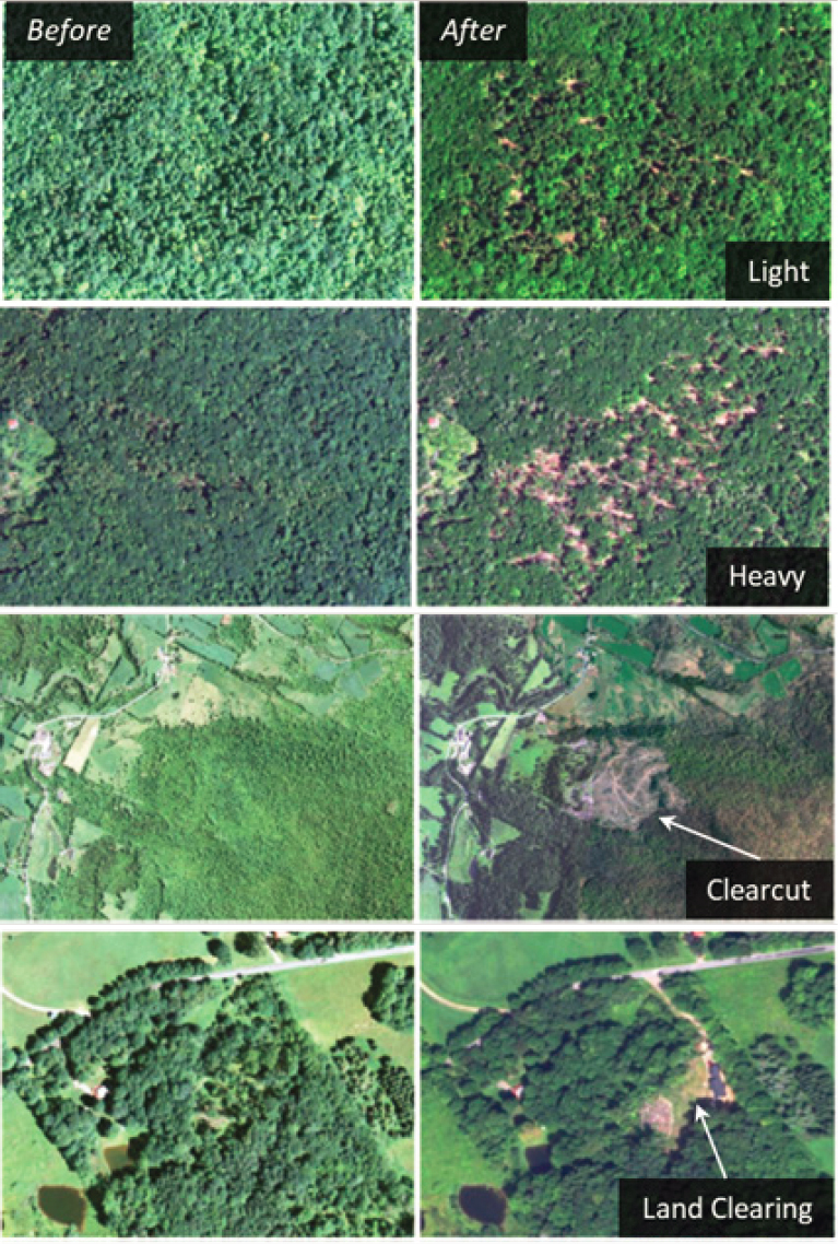
Mitigating the adverse impacts of timber harvesting and long-term conversion pressure on private forest land is the primary focus the Watershed Agricultural Council’s Watershed Forestry Program (WFP). To evaluate the influence of the WFP, VanBrakle and Pavlesich (2017, after Livengood, 2016) classified and estimated the corresponding areas of forest change in the Catskill and Delaware system. On an annual basis, they found the following logging and land-clearing activity: light (<50 percent canopy removal, 6,510 acres), heavy (50-90 percent canopy removal, 420 acres), clearcut (100 percent removal, 70 acres), and land clearing/forest conversion (100 percent/permanent removal, 57 acres). Most, if not all, of the partial cuts identified on high (1-meter) resolution digital photography (i.e., light and heavy, 93 percent and 6 percent, respectively) would not be detectable on the 30-meter-resolution Landsat imagery used for the NLCD (roughly equivalent to viewing and interpreting Figure 4-6 from 10 feet away). At 30-meter resolution, partial cuts would be classified—along with all the other undisturbed forest land—as deciduous, evergreen, or mixed forest in relation to the best-fit spectral reflectance. Clearcut areas are more likely to be accurately identified and could be classified as barren (during and shortly after cutting), herbaceous (after one growing season), or shrub cover (after two or three growing seasons) on the Landsat imagery used for the NLCD.
In most cases, land clearing is also likely to be accurately identified and could be classified as barren (i.e., an active construction site) or developed (if structures, paved areas, and/or lawns were present). The summary statistics for 15-year net loss of mature forests (categories 7, 8, and 9) for the WOH region (~7,500 acres or ~500 acres per year, Table 4-2) based on Landsat imagery are offset by the increases in herbaceous and shrub/scrub cover (~8,650 acres). Abandoned or long-fallow agricultural fields (1,660 acres between 2001 and 2016) in the Catskills quickly revert to young forests (a net change of ~7,000 acres of forest regeneration from timber harvesting). The estimate of ~130 acres of annual timber harvesting generated by VanBrakle and Pavlesich (2017) reflects the increased accuracy and precision of high resolution images (1-meter vs 30-meter) and specialized methods to detect forest change.
Detecting the land cover/land use change from (homogeneous) hay or pastureland to (heterogeneous) developed land is typically a more straightforward task than forest change detection (e.g., cutting eight or ten trees to clear a building site for a small vacation home). The total rate of conversion from forests or agricultural land to developed land estimated from the NLCD is 25-30 acres per year (0.003 percent per year) in the 1-million-acre WOH watershed. To place these observed changes in a regional context, this rate of conversion of all types is a decimal fraction of the annual loss of forest cover alone (24,000 acres, 0.075 percent) across the 32-million-acre New England region (Foster et al., 2017). Taken together, the very small changes in land cover are likely influenced by the combined effects of the Memorandum of Agreement, Watershed Protection Program, forest and agricultural land conservation efforts, and recent market trends for agricultural and forest products.
Riparian Areas in the Catskills
Riparian areas are the interface between terrestrial and aquatic ecosystems (streams, rivers, wetlands, and the shorelines of ponds, lakes, and reservoirs). In addition to providing ecological benefits, riparian buffers play a vital role in maintaining or enhancing water quality in streams. That is, the land cover and land use within
riparian areas often has a direct influence on pathways of flow and, as a consequence, streamflow and water quality. If a riparian area has deep flow paths, long residence times, and vigorous plant growth, the net effect on water quality can be quite positive. If overland flow, short residence times, and little or no plant growth predominate, the net effect on water quality is decidedly negative. Given their critical role in influencing stream water quality, mapping, assessing, and protecting riparian areas are foundational components of any watershed protection program.
The reference condition for riparian areas in the Catskills is forest vegetation. Nonetheless, the site-specific diversity, character and condition of the riparian plant community varies in relation to land use history, soil characteristics, terrain features, seasonal inundation (if any) and effective rooting depth, and the dynamic interaction with the stream channel. The NYC DEP very conservatively estimates the total riparian area in the WOH watersheds to be 239,400 acres—one-fourth of the total watershed area. This estimate is derived using a 300-foot “programmatic” buffer on both sides of a very detailed stream network map (3,688 miles WOH, developed from high-resolution LiDAR and digital orthophoto data and terrain analysis in GIS). A 50-foot buffer would reduce this estimate to approximately 40,000 acres (~4 or 5 percent of the watershed area). Public (protected) land comprises 34 percent of the riparian area and is 99 percent forested, while private land comprises 66 percent of the riparian area and is 91 percent forested. The remaining land cover within private riparian areas is ~4 percent turf or soil and ~5 percent developed land (some of which is impervious surface). Note, however, that the proportions of public versus private land in the 300-foot regulatory buffer varies substantially across the six WOH watersheds. The highest proportions (56 percent in the Ashokan watershed, 57 percent in the Neversink watershed, 48 percent in the Rondout watershed) reflect the protection conferred by the Catskill Forest Preserve in their headwater areas and the high-priority focus of the NYC DEP Land Acquisition Program in these terminal reservoir watersheds. In contrast, the smallest proportions of public land occur in the Cannonsville (20 percent), Pepacton (28 percent), and Schoharie (30 percent) watersheds.
Protecting or restoring riparian forest buffers can be one of the most cost-effective ways to maintain or enhance water quality in streams, and it plays a role in several of the programs discussed in subsequent chapters, including the Watershed Agricultural Program (Chapter 5), the Stream Management Program (Chapter 6), and the Land Management Program (Chapter 7). Many watershed management projects seek to maintain or restore 75 percent coverage of riparian forest buffers—often requiring decades of work and thousands of stream miles to reach this goal (e.g., the Chesapeake Bay Program5). Hence, the high percentage of forested riparian buffers on publicly owned land in the WOH watersheds provides an excellent initial condition for further protecting the water supply from those watersheds. Riparian forest buffer establishment and livestock-exclusion fencing are routinely included in Whole Farm Plans, using the USDA Conservation Reserve Enhancement Program (CREP) and modest annual payments for land removed from agricultural production. For other parts of the WOH watershed, NYC DEP funds the Catskill Streams Buffer Initiative (CSBI, established in 2009). These activities are discussed in detail in subsequent chapters.
POLLUTANTS IN THE WATERSHED AND THEIR SOURCES
In NRC (2000a), four priority pollutants were ranked according to the threat that they posed to the NYC water supply. That report concluded that the watershed management program should be prioritized to place importance first on microbial pathogens, second on organic precursors of disinfection byproducts, third on phosphorus, and fourth on turbidity and sediment. In the intervening 20 years, it is clear that these priorities have been addressed, particularly the emphasis on microbial pathogens with the construction of the ultraviolet (UV) disinfection plant. Today, turbidity, nutrients, and dissolved organic matter are higher-priority threats to the quality of the water supply, especially given the potential increases in precipitation and stream flow likely to be observed in the near future. Because various land uses in the watershed can be sources for many pollutant types, all of the remedial watershed protection programs are required to control the sources of these four major pollutant categories (as shown in Table 4-6). Nonetheless, control of sediment is largely discussed in Chapter
___________________
6 under the Stream Management Program. Nutrients, particularly phosphorus, are a major focus of Chapter 5 on the Watershed Agricultural Program. Dissolved organic carbon is discussed in Chapter 10 on the Forestry Program. And microbes are discussed primarily in Chapter 11 on waterborne disease surveillance, microbial pathogen monitoring, and the waterfowl program. The entire suite of pollutants is touched on in Chapter 8 on wastewater treatment and in Chapter 9 on stormwater management. Chapter 10 tackles invasive species, both terrestrial and aquatic, that have emerged as concerns over the last decade.
Turbidity
Turbidity, a measure of water’s relative clarity, is caused by fine particles of suspended sediment (clay, silt, and fine sand), small particles of organic and inorganic matter, and microscopic organisms including algae, plankton, and others. Turbidity is measured as the amount of light scattered (at 90 degrees) by these particles in water, and is reported in nephelometric turbidity units (NTU). Highly turbid water is aesthetically unappealing and possibly a cause for health concerns in drinking water, particularly because particles in water can absorb other pollutants (notably metals, nutrients, and bacteria) and shield pathogens from disinfection.
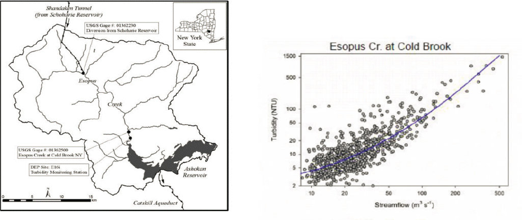
Although turbidity varies along streams both in time and space (e.g., by reach), higher values of turbidity generally are associated with elevated flows in streams (Figure 4-7; Effler et al., 1998; McHale and Siemion, 2014). When stream discharge is high, the water moves at a higher velocity, leading to erosion of sediment from the bed and banks and also facilitating the downstream transport of these sediments. In the parts of the watershed with the highest turbidity values (areas draining to the Ashokan Reservoir) the bed and bank sources of sediment are more significant than the upland sources of sediment. Suspended sediment (or suspended solids) concentrations are linked closely to turbidity values, and the two were correlated by repeat sampling and development of a calibration curve for a particular waterbody (McHale and Siemion, 2014). These two
TABLE 4-6 Primary Pollutants of Concern, Sources, and Remedial Programs
| NYC DEP Program | Pollutant Sources | Sediment | Nutrients | Pathogens | DOM | Toxics |
|---|---|---|---|---|---|---|
| Agriculture Program | Manure | X | x | x | ||
| Row-crop farming | x | x | x | |||
| Dairy/cattle pasture | x | x | x | |||
| Stormwater Program | Construction sites | x | ||||
| Urban developed land | x | x | x | x | ||
| Stream Management Program | Channel erosion | X | ||||
| Wastewater Treatment Program | WWTP effluent | x | x | x | ||
| Septic Tank Program | Failed septic tanks | x | x | x | ||
| Forestry Program | Land surface erosion/plant matter | x | x |
NOTE: The table is not meant to be a treatise on how well the individual programs work.
Bold and capital X’s indicate a more important source of the pollutant relative to other sources.
DOM = dissolved organic matter.
SOURCE: Mukundan (2019).
measures are not the same, however, as suspended solids are a measure of mass (related to particle volume) and turbidity is more closely related to particle surface area; hence, turbidity emphasizes smaller particles that are much less likely to settle.
In the various reservoirs of the NYC water supply system, turbidity can change, sometimes dramatically, at time scales of minutes to hours and be quite different in one reservoir relative to another. Because maintaining the turbidity in the final product water that enters the NYC distribution system is so critical, NYC DEP has spent considerable effort studying and documenting the causes of elevated turbidity in several reservoirs. Studies performed approximately 20 years ago (e.g., Effler et al., 1998; Peng et al., 2002, 2004) made it clear that episodes of high turbidity were caused by erosion of stream beds and banks, particularly when that erosion penetrated into glacio-lacustrine sediments. In particular, sections of Esopus Creek were delineated as the primary source of the highly turbid water entering Ashokan Reservoir.
As discussed in Chapter 3, turbidity in the finished water should not exceed 5 NTU, the upper limit specified in the Surface Water Treatment Rule (SWTR) for filtration avoidance. As shown in Figure 4-8, the 5-NTU limit at DEL18 has not been exceeded in the last 18 years, with the closest call occurring in September 2011 just following Tropical Storms Irene and Lee. Addressing the turbidity concern requires that NYC DEP (1) identify sources of high turbidity, (2) determine mitigation strategies to reduce incoming turbidity from those sources, and (3) develop procedures to manage reservoir turbidity if it is high. NYC DEP has studied and implemented mitigation strategies and invested in major infrastructure changes throughout their system to minimize the possibility of an exceedance of the turbidity limit. If the turbidity in water approaching the Kensico Reservoir is (or is expected to be) too high, the final stop-gap measure is to add alum at the Catskill Influent Chamber to allow flocculation to occur in the pipeline prior to water entering Kensico Reservoir. This process agglomerates a large number of small, nearly unsettleable particles into far fewer and larger particles that settle out in the upper reaches of the Kensico Reservoir. Since 1986, alum has been used for flocculation of particles in the Kensico Reservoir about a dozen times, with the most recent use in 2011/2012 during the aftermath of Tropical Storms Irene and Lee (Table 4-7).
As indicated by the entries in Table 4-7, the water with high turbidity, when it occurs, is in the Ashokan Reservoir. The first step that the NYC DEP took in 1996 was to study in detail the possible sources of turbid-
SOURCE: Plotted by the Committee from data provided by NYC DEP.
ity in the Ashokan Reservoir, which receives water not only from its own watershed but also from Schoharie Reservoir. Water transferred from the Schoharie travels 18 miles through the Shandaken Tunnel before being discharged to the Esopus Creek, and then flows 12 miles in that natural stream before entry into the Ashokan Reservoir. The conclusion of the 1996 study was that the primary source of the high turbidity in Esopus Creek during and immediately following storm events was not the Schoharie Reservoir water but rather the streams draining the Ashokan watershed itself. As discussed in greater detail in Chapter 6, the high turbidity was ascribed to the erosion of clay soils (especially in stream beds and embankments) and the type of geologic units in the watershed.
The NYC DEP subsequently undertook the extensive Catskill Turbidity Control Study, which was completed in 2008 (NYC DEP, 2008). This study had three major phases and investigated numerous possibilities for improving the water quality and/or reducing the water quantity that would enter the Catskill Aqueduct from the Ashokan Reservoir. Some options were eliminated from further consideration because they were deemed likely to be ineffective, and others were eliminated because of high costs (e.g., installing baffling throughout the Ashokan Reservoir to allow more particles to settle prior to the entrance into the Catskill Aqueduct). As described in Chapter 3 of NASEM (2018), the major changes that were undertaken (and that are now completed) were as follows:
- Turbidity source control measures in the Schoharie and Ashokan watersheds;
- Infrastructure improvement, primarily in the Catskill Aqueduct; and
- Operational changes, primarily supported by the development of a major modeling effort called the Operations Support Tool (OST).
Despite these improvements and changes, in the Committee’s opinion, turbidity will remain a significant challenge for the NYC water supply for the foreseeable future. This conclusion stems from the presence of a low turbidity target for Kensico Reservoir, the nature of the sources of turbidity in the Catskill system, the uncertainty about how restored stream corridors will fare during future extreme events, and the existence of the Croton filtration plant and the UV plant, which have reduced the threat of microbial pathogens. The Stream Management Program was created primarily to deal with this turbidity issue, but it is too soon to say how effective it will be (see Chapter 6). The development of the OST has been a major accomplishment that provides a systematic procedure for operating the various possible levers in the entire NYC drinking water
TABLE 4-7 Alum Use in the Catskill Aqueduct to Reduce Turbidity Since 1986
| Year | Start Date | Days Used | Reason | Alum Dose (ppm) | Total Alum Used (lbs) |
|---|---|---|---|---|---|
| 1987 | 4/6/1987 | 43 | Turbidity | 5-15 | 921,680 |
| 1996 | 1/22/1996 | 151 | Turbidity | 8-15 | 2,477,954 |
| 1997 | 1/14/1997 | 15 | Turbidity | 7-8 | 237,046 |
| 2001 | 1/10/2001 | 23 | Turbidity | 7-8 | 482,226 |
| 2005 | 4/5/2005 | 76 | Turbidity | 6-15 | 1,740,393 |
| 10/13/2005 | 41 | Turbidity | 7-9 | 7,383,144 | |
| 2005-2006 | 12/1/2005 | 129 | Turbidity/Gilboa Dam Repairs | 7-11 | |
| 2006 | 5/15/2006 | 10 | Turbidity | 7 | |
| 6/28/2006 | 36 | Turbidity | 7-16 | ||
| 2011 | 1/31/2011 | 11 | Turbidity from 2010 Storms | 5-7 | 208,462 |
| 3/2/2011 | 79 | Turbidity | 6-14 | 1,238,790 | |
| 2011-2012 | 8/29/2011 | 260 | Turbidity | 7-23 | 5,950,055 |
SOURCE: NYS DEC (2017).
network to minimize the risk of violating the turbidity standard. High turbidity negatively impacts the effectiveness of the UV disinfection facility, both because of reduced light penetration and because microbes attached to other particles might be shielded from the UV radiation.
Nutrients and the Trophic State of the Reservoirs
The trophic state of the reservoirs has been a long-standing concern of the NYC DEP (see the annual NYC DEP water quality reports; NRC, 2000a). Eutrophic conditions result from increased nutrient loadings to the reservoirs, particularly phosphorus (Auer et al., 1998; Doerr et al., 1998), and present a number of challenges from the perspective of drinking water quality. First, the algae in a eutrophic reservoir results in an increase in turbidity, which, as discussed above, is an important type of impairment that could lead to a determination that filtration is required. Second, the algae and the biomass of dead algae that can result from a large bloom can lead to a substantial increase in total organic carbon in the reservoirs because the algal population causes large amounts of carbon to be fixed from the atmosphere by photosynthesis. As discussed later, high concentrations of organic carbon can lead to the formation of disinfection byproducts (DBPs).
Third, the taste and odor problems associated with algal blooms and/or large die-offs of algae are detrimental to public acceptance of the water, even if it is not in violation of health requirements. If eutrophication were to cause taste and odor problems it would be a major setback for the public support for the system. Fourth, highly eutrophic water can lead to the growth of cyanobacteria, which can produce microcystins or other compounds toxic to humans who come into contact with them or consume them in drinking water. If harmful algal blooms (HABs) became common in the NYC reservoirs, it would almost certainly force filtration, which would be an effective approach to handling HABs and rendering the water safe for human consumption. There could be other treatment options for HABs but certainly avoiding HABs is an important part of avoiding the need for filtration.
Finally, massive algal die-offs are a common feature of eutrophic waterbodies, and the potential for anoxia or hypoxia that results from these die-offs can be a detriment to fish populations (and hence to recreational use of the reservoirs). In addition, the lack of dissolved oxygen in bottom water can lead to the enhanced recy-
cling of previously deposited phosphorus in lake-bed sediments (Bostrm et al., 1988; Nürnberg, 1994; Sharpley et al., 2013). Thus, eutrophication can continue to harm the quality of a reservoir for many years after the inputs of nutrients have been reduced. This positive feedback mechanism heightens the importance of reducing phosphorus inputs before conditions get out of control, because the process is not easily reversed.
Trophic State Index and Phosphorus Concentrations
NYC DEP uses a trophic state index (TSI) developed by Carlson (1977) which classifies each reservoir for each year according to the chlorophyll a concentrations observed during the growing season. Using this median value of the TSI for a given reservoir for a given year, they define oligotrophic conditions as values of 40 or less, and eutrophic conditions as values of 50 or more, with those that lie between 40 and 50 classified as mesotrophic. Among the WOH reservoirs, Cannonsville was the one reservoir in the eutrophic category in 2017, and no other reservoir had a value in the eutrophic range at any time in the period 2007-2017. Cannonsville had TSI values substantially higher than the other reservoirs during this period.
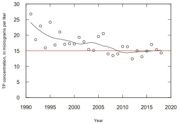
Another indicator of eutrophication is the phosphorus concentration in the water column in the reservoirs. The limiting nutrient for biological growth in the NYC reservoirs is phosphorus (NYC DEP, 1999). Although a guidance value of 20 μg/L was used during the Phase I phosphorus total maximum daily load (TMDL) work of the late 1990s, analysis by NYC DEP (1999) indicated that a guidance value of 15 μg/L was needed to ensure high-quality drinking water for the City, and it used this level for the Phase II TMDLs, which NRC (2000a) strongly endorsed. Among the WOH reservoirs, the only one that has recently experienced eutrophic conditions is Cannonsville. Figure 4-9 shows the mean concentrations of phosphorus in Cannonsville Reservoir for the growing season (sampled over all depths and sampling sites) for the period 1991-2018.
Figure 4-9 clearly shows that when significant investments were being made in wastewater treatment plant (WWTP) upgrades (up through 2003), the reservoir total phosphorus (TP) values were generally falling, and that trend may have continued through approximately 2008 (with the lag likely related to recycling of phosphorus in the reservoir bed for a few years after completion of the WWTP upgrades). But the most recent part of the record (2012–2018) shows, at least subjectively, a small rise in phosphorus concentrations. What is certain is that the typical annual values of TP concentration are about evenly distributed around 15 μg/L. A linear regression to test for trends from 2008 to 2018 reveals an estimated slope of +0.083 μg/L/yr, which is not statistically significant. However, the likelihood that the true trend is upward is 0.71, while the likelihood that it is downward is 0.29. These results suggest that watershed protection strategies, at least over the 2008-2018 period, do not seem to be resulting in progress in terms of reducing this indicator of eutrophication in Cannonsville Reservoir.
Monitoring of Algal Toxins
Another important line of evidence regarding the trophic state of the reservoirs comes from monitoring of algal toxins. Monitoring in 2017 showed positive results in four reservoirs (Cannonsville, New Croton, Croton Falls, and Diverting), although the report did not indicate the number of samples taken from these reservoirs or the total number of reservoirs sampled, making it difficult to put the following data into context (NYC DEP, 2018a). The samples were taken mostly in areas that presented visual evidence of a possible toxic algal bloom, rather than from a designed sampling network. Anatoxin-a was detected in these four reservoirs, while microcystin-LA was detected in Croton Falls and Cannonsville. Two microcystin-LA measurements in Cannonsville had concentrations of 1.9 and 459 μg/L. The EPA health advisory levels for microcystin are 0.3 μg/L for preschool-age and younger children and 1.6 μg/L for older children and adults.6 The NYS DEC criteria for a “high toxin bloom” is 10 μg/L. This finding of microcystin at a level more than two orders of magnitude above the adult health advisory is concerning, and the Committee is not aware of any plans by NYC DEP to increase monitoring for algal toxins.
At this time, no national data set tracks the number and magnitude of HABs, but the perception by experts is that they are becoming more widespread and severe in lakes and reservoirs. Notable examples in North America are Lake Erie, Lake Champlain, and Lake Winnipeg. Huisman et al. (2018) found “evidence indicating that cyanobacterial blooms are increasing in frequency, magnitude and duration globally” and suggest that both “eutrophication and climate change catalyse the global expansion of cyanobacterial blooms.” Paerl and Huisman (2008) clearly show that increasing water temperature makes conditions more favorable for blooms. It is likely that a longer ice-free period in lakes is having an effect of increasing the intensity and duration of cyanobacter blooms (see Paerl et al., 2019; Smol, 2019). Smol (2019) also notes that “there has been a significant rise in the number of confirmed cyanobacterial bloom reports [in the Canadian Province of Ontario] since the 1990s, and many are from remote lakes that are oligotrophic or have not experienced nutrient fertilization.” He suggests that climate trends may be driving this recent increase and may be of greater importance than any phosphorus input trends. The implications of climate change for toxic cyanobacteria blooms are discussed by Paerl et al. (2019).
Because of climate change, cyanobacteria blooms are generally an increasing threat to lakes and reservoirs, which could be highly relevant to the NYC reservoirs, particularly Cannonsville. Even in the absence of future increases in phosphorus input to the reservoirs, longer ice-free periods, higher water temperatures, and the potential for increased internal loading of phosphorus (from bottom sediments) could increase the threat of HABs over time.
Analysis of Phosphorus Data Upstream of Cannonsville
NRC (2000a:164) states that “the suppression of phosphorus loading rates to the Catskill/Delaware reservoirs is a particularly important goal for the New York City watershed management strategy.” This Committee strongly endorses that statement and further notes that the data on trends in trophic state, reservoir phosphorus concentrations, and new indications of algal toxins place a particularly high priority on the need to suppress phosphorus loading rates to the Cannonsville Reservoir. Thus, the Committee explored the question of whether phosphorus loading rates since 2000 have indeed been suppressed.
The full data set used in this analysis consisted of 5,094 samples of TP concentration collected by NYC DEP from the West Branch of the Delaware River at Beerston, over the period water years 1988 through 2018 (an average sampling frequency of about 13 samples per month), in conjunction with daily discharge data from the USGS streamgage at this location. The sampling done by NYC DEP was ideally conducted for estimating nutrient fluxes. The sampling covered all seasons and all flow conditions but it placed substantial emphasis on sampling at the highest discharges (when nutrient fluxes are highest). For example, 6.7 percent of the samples in this data set were collected on days when discharge was higher than the 99th percentile on the distribution of
___________________
6 See https://www.epa.gov/cyanohabs/epa-drinking-water-health-advisories-cyanotoxins.
daily discharges. The Beerston monitoring site is just upstream of Cannonsville Reservoir. The drainage area at the monitoring site is 352 mi2, which is 77 percent of the total drainage area of the reservoir. No significant point sources of phosphorus exist between the monitoring site and the reservoir. Thus, data from this monitoring site provide a good representation of phosphorus inputs to the reservoir.
The discussion starts with an analysis of the entire period (1988-2018) in order to place the specific question about trends from 2000 to 2018 in a larger context. The approach used in this analysis was weighted regressions on time, discharge, and season (WRTDS) (Hirsch et al., 2010). WRTDS is designed to describe and evaluate river water quality trends in a manner that removes the influence of the year-to-year variability of weather conditions to increase the signal-to-noise ratio, thereby improving trend description. This method decreases the potential of reaching false conclusions about long-term trends that arise from a pattern of particularly wet or dry years in the early or late portions of the record analyzed. NYC DEP has begun using WRTDS in analysis of their river water quality data although they have yet to use it in any of their reports. Because of the growing importance of changing streamflow conditions in recent years, the WRTDS method has been recently enhanced with the introduction of “generalized flow normalization” (Choquette et al., 2019), which removes the influence of year-to-year variations in streamflow but does consider the potential influence of long-term trends in streamflow on the resulting water quality trend estimates.
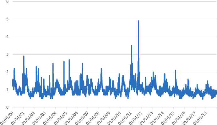
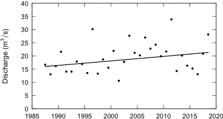
The Committee’s analysis of the streamflow record for the West Branch of the Delaware River at Beerston indicates an increase in mean discharge of about 33 percent over the three decades of water quality sampling considered here (almost significant at the 0.1 alpha level). Figure 4-10 shows the annual mean discharge record from January 1988 through December 2018. This increase in average streamflow is an important component in the overall change in TP flux in the West Branch of the Delaware River above Cannonsville Reservoir.
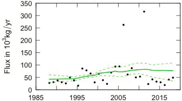
The Committee’s analysis of TP flux is shown in Figure 4-11. The flow-normalized flux increased from 42 metric tons per year in 1988 to 77 metric tons per year in 2018, an increase of 82 percent. One can apportion that change between the part of the trend that is a result of the changes in streamflow and the part that is a result of changes in the relationship between concentration and discharge. The results indicate that the increasing streamflow over the period accounts for a 31 percent increase and the changing relationship between concentration and discharge accounts for a change of 51 percent in TP flux. Thus, averaged over all times of the year
and all flow conditions, the water flowing past this monitoring station carries an increasing amount of TP for any given discharge. And, the increases in the magnitude of discharge over the period have further increased the rising average level of annual flux.
It is worth noting that during this period the WWTP flux of phosphorus in this watershed decreased quite substantially. Between 1990 and 2003, the flux of phosphorus from WWTPs decreased by about 99 percent or more, and all of the significant WWTPs in the Cannonsville watershed lie upstream of the Beerston monitoring site. However, these WWTP decreases amount to only about 12 metric tons per year, a relatively small amount compared to the estimated flux of about 80 metric tons per year in recent years. The WWTP reductions have been very worthwhile, particularly in reducing phosphorus concentrations during periods of low flow, in reducing the soluble phosphorus concentrations during these periods, and reducing the risk of pathogens entering the reservoir, but from the standpoint of TP fluxes into Cannonsville, they represent only a minor decrease. The dominant drivers of TP in the watershed are clearly nonpoint sources and the increasingly wet climate.
The black dots in Figure 4-11 show the estimates of annual flux of TP at the site, based on the daily discharge record and the WRTDS statistical model of concentration as a function of time, discharge, and season. Note that year-to-year the flux varies by more than an order of magnitude, with most of that variation being a function of the hydrologic conditions for the year (high flux values corresponding to years of very high discharge). For example, the two very high values are in water years 2006 and 2011, which are the two highest discharge years in the 31-year record. The green line represents the flow-normalized flux, which is the expected value of flux for each year, computed in a manner that removes the influence of the year-to-year variations in discharge, but not the seasonality or trend in discharge. The flow-normalized flux curve as computed is substantially higher than the annual flux estimates for 2012 through 2018 because it combines results from the very high flux years, 2006 and 2011, with the much lower flux years of 2012–2018. The green dashed lines represent the 90 percent confidence interval on the flow-normalized flux (the method for computing these confidence intervals is described by Hirsch et al., 2015). Note that the flux is substantially more uncertain near the beginning and the end of the record, and that the uncertainty band becomes wider as the expected value increases. The uncertainty of the overall trend in the flow-normalized flux is that it is “likely” that the trend is upward over this full period,7
___________________
7 Terms such as “likely” are quantitatively defined in Hirsch et al. (2015).
and the likelihood that the trend over this period is upward is about 0.78 (and thus the likelihood that the trend is downward is 0.22).
It may seem odd that although the increase over the full period seems rather obvious when looking at the graph, the uncertainty about the trend is substantial. One’s eyes, when observing the graph, are likely to focus on the period from about 1995 to about 2010 when the flow-normalized flux values are pretty clearly increasing and the confidence intervals are relatively narrow. Running an uncertainty analysis on just the period 1995-2010 reveals that the upward trend for this shorter period is “highly likely” (likelihood that it is an upward trend being 0.99). Indeed, the real story is one of relatively small increases in the period up to about 1995, followed by a period of steep upward trends until about 2010, followed by a flat or possibly declining period since then (change in flux from 2010 to 2018 is estimated at -5 percent and the likelihood that it is truly a down trend is about 0.75). Understanding what lead to the steep increase from 1995 to 2010 followed by the leveling off since then could help to illuminate the best control strategies for the future.
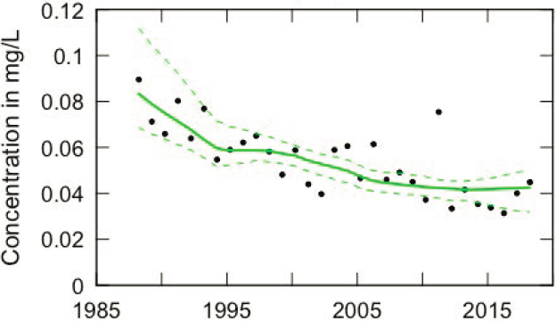
WRTDS can also consider the trend in the flow-normalized annual mean TP concentration for the same 1988-2018 period, shown in Figure 4-12. In Figure 4-12, the estimated mean annual concentrations are shown as the black dots, the flow-normalized annual mean concentration are shown by the green line, and the dashed green line show the 90 percent confidence interval on the flow-normalized concentrations. This graph clearly reveals the impact of the WWTP reductions mentioned above. The flow-normalized annual mean concentrations decline over the 1988–2018 period from 0.083 to 0.042 mg/L, a decline of 49 percent. This decline is almost entirely driven by the change in the relationship of concentration to discharge (waters becoming more dilute over time). The component of change due to the change in discharge is negligible. The uncertainty analysis for flow-normalized concentration indicates that a downward trend in concentration is highly likely (with a likelihood value of >0.99).
How should one interpret the apparent contradiction between the trend results for flux (upward but rather uncertain) versus the trend results for concentration (downward and highly certain)? The difference arises because the mean concentration over this period reflects the decline in concentration on the many days of the year when discharge was relatively low (not influenced by storms or snowmelt events). This decline is a result of the decreased TP concentration associated with the WWTP upgrades that took place in the early part of this record. In contrast, the change in flux is much more influenced by the relatively few days of the year when
discharge was high. The concentrations at high discharges are strongly determined by nonpoint-source contributions of TP. The substantial improvement associated with the WWTPs is of limited consequence to flux on those days, because the river discharge is dominated by runoff from the landscape and not WWTP effluent. The uncertainty in estimates of concentrations at low flow is much less than the uncertainty in estimates of concentration at high flow. The consequence of this is that the 90-percent confidence bands around the estimates are much narrower (in relation to the mean) for the concentration estimates than for the flux estimates. The most important point here is that trends in concentration and trends in flux may be quite different from each other. Thus, analysis of trends in concentration is not necessarily a good indicator of the trends in flux.
From the standpoint of the nutrient availability in the reservoir, the appropriate measure of change is the flux change and not the concentration change. What matters to the ecological processes in the reservoir is the mass of phosphorus in the inputs to the reservoir averaged over a period of several months to a few years. That mass is dominated by what enters the reservoir on high-flow days. The decreases in concentration that have occurred on medium to low-flow days constitute a very minor change in the overall mass of phosphorus entering the reservoir over periods of many months to a few years. What these analyses convey is that although average concentrations have declined over time (probably mostly driven by WWTP improvements), the flux has probably increased over time. That increase was steepest during the period from about 1995 to 2010 and the last decade or so shows no clear evidence of increase or decrease in flux.
Returning to the original proposition about “suppression” of loading rates (fluxes) since the time of the previous report, one can focus the analysis on the specific period of water years 2000 to 2018. The best estimate of change in flux over this period is an increase of 16 percent, and this change is equally divided between a component associated with increasing streamflow and a component due to the generally higher concentration values for any given discharge. However, the uncertainty analysis conveys that the likelihood that the true trend is upward is almost exactly 50 percent and that the true trend is downward is also 50 percent. In other words, the empirical data indicate about a 50-50 chance that phosphorus loads to the reservoir have indeed been suppressed over the time since that study, and the best estimate is that it has slightly increased rather than decreased. In contrast to this result, the best estimate of the change in mean concentration is a decrease of about 25 percent over this period and it is virtually certain that the change is indeed a decrease. Further analysis of the most recent part of the flux record (from 2008 to 2018) provides an indication of a pattern of decrease, but the likelihood that it is indeed a decrease is about 0.67 and the amount of change over this period is only about 2 percent, from 78.8 in 2008 to 77.3 metric tons per year in 2018.
The Committee’s analysis suggests that continued efforts to limit TP fluxes may be reversing the previous pattern of increase and could even be turning it around. The uncertainty analysis indicates a likelihood of 0.9 that progress is being made in the past decade compared to the previous one. Progress is defined here as one of three possibilities: (1) the trend in the first decade was upwards and the trend in the second decade was downwards (likelihood = 0.65); (2) the trend in the first decade was upward and the trend in the second decade was also upward but less steeply (likelihood = 0.24); or (3) the trend in both decades was downward but it was more steeply downward in the second decade (likelihood = 0.01). The bottom line is that there is a reasonably strong indication that the TP flux trends are moving in the right direction, but the rate of improvement is very slow.
The Cannonsville watershed is not unique in the slowness of watershed-scale response to nonpoint source phosphorus management controls. Smith et al. (2019) points out that the disconnect between field-scale effort and watershed-wide results “can arise from inadequate intensity and insufficient targeting of BMPs.” The disconnect can also be a result of the “lags associated with the continued chronic release of legacy phosphorus from past management” as well as stored phosphorus in soils and sediments throughout the watershed. All of this can cause impairments to continue “at timescales of years to decades and longer.”
The Committee’s conclusion is that these various lines of evidence about eutrophication, toxic algae, and river nutrient fluxes, at least in the Cannonsville watershed, all fail to provide clear indications that the current set of strategies for reducing the risk of eutrophication is having a substantially positive impact. Understanding the changing conditions in the watersheds above each of their reservoirs, the phosphorus fluxes into the reservoirs, and the ecological conditions in the reservoirs needs increased attention from NYC DEP. At least for Cannonsville, but to a lesser extent some other watersheds, NYC DEP needs to consider the introduction of
new strategies to substantially decrease the risks associated with eutrophication of the reservoir. Other chapters of this report suggest some potential strategies.
Natural Organic Matter
Natural organic matter (NOM) is found in essentially all natural waters, especially surface waters; it stems from the decay of leaves and plants primarily, but also from animals, microorganisms, and fish. Synthetic organics can also make their way into surface waters from a variety of sources, including direct runoff of stormwater and from wastewater treatment plants if the organics are not (or only partially) degraded. In most natural waters, the concentration of NOM far exceeds that of synthetic organics, so that a measure of total organic carbon (TOC) is taken as the NOM concentration.
Carbon is also present in virtually all natural waters as inorganic carbon: the soluble species of carbonic acid (H2CO3, which is essentially dissolved CO2 gas), bicarbonate (HCO3–), carbonate (CO32–), and insoluble metal carbonates (with calcium carbonate, CaCO3, being the most common and abundant). TOC is measured by oxidizing all organic material by one of a few different methods, leading to the production of carbon dioxide. This carbon is measured and, after accounting for the initial inorganic carbon present in the water, is reported as the TOC. Often, a sample is filtered through a membrane filter prior to measurement and, in that case, the measure is known as the dissolved organic carbon, DOC. For many years after the concern about organic carbon in drinking water supplies was first raised, the NYC DEP measured and reported both TOC and DOC, but the differences were so infinitesimal that they now measure only DOC but report it in the annual drinking water quality reports as the TOC. Further, since the concentration of synthetic organic compounds is extremely low in the NYC DEP system in comparison to the natural organics, the TOC measurement is interpreted to be the NOM concentration.
NOM (measured as DOC or TOC) is rarely, by itself, a problem in water. However, it can react with disinfectants used in drinking water treatment to create DBPs, which can be carcinogenic (reviewed in Reckhow and Singer, 2011). When chlorine is used as the disinfectant (as it is by NYC), a huge variety of chlorinated (and otherwise halogenated) organic species can be formed. When chlorine gas is dissolved in water, it rapidly dissolves to form hypochlorous acid and hypochlorite (OCl–), with the mixture of the two dependent on pH. If bromide is present in the water, these chlorine compounds can oxidize the bromide to hypobromous acid (HOBr) and hypobromite (OBr–); these species are also oxidants and hence can react with the NOM just like chlorine, which is why the DBPs that are formed can incorporate bromine as well as chlorine. Similar reactions can occur with iodide but this halogen is rarely present in significant quantities and thus iodated compounds are usually of little consequence.
A highly simplified, yet nevertheless instructive, view of the reaction is as follows:
NOM in water + chlorine → DBPs
This equation is useful because it makes clear that only three methods are available to limit the DBP concentration in finished water that reaches the consumer:
- Choose a water source that has a low (reactive) NOM content, or remove some fraction of the NOM in treatment,
- Use an alternative disinfectant besides chlorine, or
- Allow the DBPs to form and then remove them.
All three of these DBP control measures are used widely in the United States by drinking water utilities. The NYC DEP is quite fortunate that its water sources have relatively low concentrations of DOC and so, at least to date, they have not been forced to remove NOM, use an alternative disinfectant, or remove DBPs after formation. (The good fortune is no accident, given that the decision makers, even long ago when the early
reservoirs were sited, knew that they were choosing locations with high-quality water; however, these decisions were made decades before the problems of DBPs were first recognized in the early 1970s.)
The NYC DEP monitors DOC concentration often at various points in the vast reservoir system; data from several key locations are shown in Figure 4-13; in most cases, the data were recorded weekly at these eight locations. For clarity, the data are shown in four parts, with parts A and B showing data from the Delaware system and parts C and D showing data from the Catskill system (or in the case of DEL18 shown in part D, water that is a blend from both systems). Except data from the SRR2CM site, a high fraction of the data points are below 2.0 mg/L and all but a few are below 2.5 mg/L. The values at SRR2CM are often much higher and reflect the different nature of the forested lands surrounding the Schoharie Reservoir, which is the northernmost part of the Catskill system. Fortunately, that water is mixed with the much greater amount of water that enters the Ashokan Reservoir, so that the blended water (at EARCM, also shown in Part C of the Figure) is nearly always below 2 mg/L. For surface water systems using conventional filtration, the EPA has regulations and treatment requirements for supplies that routinely have DOC values in excess of 2.0 mg/L. While this requirement is not directly applicable to NYC’s unfiltered system, as the data in Figure 4-13D show, the NYC DEP is generally, but not always, below that value in the water leaving Kensico.
The NYC DEP also monitors DOC concentrations within the distribution system, and summary data for the past six years are shown in TABLE 4-8. These data show that the average value has consistently been below 2 mg/L throughout the time period shown. The data also show, however, that the maximum readings each year are above 2.0 mg/L; the higher values are an indication that the creation of DBPs is possible within the distribution system.
Of the wide variety of halogenated organics formed as DBPs, two groups are usually dominant on a mass basis, and their concentrations are regulated in drinking water by the EPA. Those two groups of compounds are the trihalomethanes and some of the haloacetic acids. The trihalomethanes are chloroform (CHCl3), dichlorobromomethane (CHCl2Br), dibromochloro-methane (CHClBr2), and bromoform (CHBr3). The regulatory limit for the sum of the concentrations of these four compounds is 80 μg/L; how this limit is applied is shown below. The second group of regulated DBPs is a set of five haloacetic acids; acetic acid is CHCH3 and a haloacetic acid is formed if one, two, or all three of the hydrogen atoms on the right end of that formula is replaced by chlorine and/or bromine. Nine such species are possible, but only a subset of five (monochloroacetic acid, monobromoacetic acid, dichloroacetic acid, dibromoacetic acid, and trichloroacetic acid) are included in the regulation (which stems from the fact that no reliable methodology for measuring the other four was available when the regulation was promulgated). The regulatory limit for the sum of the concentrations of these five compounds is 60 μg/L.
The formation of DBPs is a slow process; some of these regulated DBP compounds (as well as a far greater number of unregulated DBPs) are formed in a very short time after the addition of chlorine, but the formation continues to occur throughout the distribution system over the course of several days. In light of this fact and for the protection of the public health, the EPA regulations specify that samples must be measured at several locations throughout the distribution system on a quarterly basis, and the running average of four consecutive measurements at any one location cannot exceed the values noted in the previous paragraph. The locations must be approved by the governing authority (NYS DEC in the case of NYC) and must be chosen to reflect the likelihood of finding the maximum concentration of these regulated DBPs. Each quarter, the utility must report to the primacy agency the locational running annual average (LRAA) for every location.
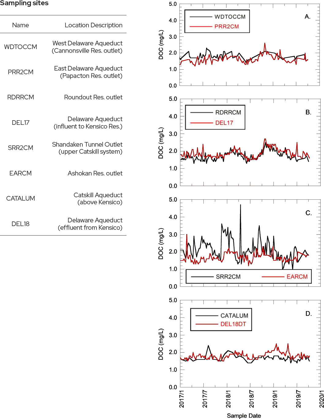
TABLE 4-8 Dissolved Organic Carbon in the NYC Distribution System
| Year | Sample Numbers | Range (mg/L) | Average (mg/L) |
|---|---|---|---|
| 2013 | 273 | 1.3 – 1.8 | 1.5 |
| 2014 | 272 | 1.3 – 1.7 | 1.5 |
| 2015 | 291 | 1.3 – 2.1 | 1.6 |
| 2016 | 304 | 1.3 – 2.4 | 1.6 |
| 2017 | 350 | 1.3 – 2.1 | 1.5 |
| 2018 | 459 | 1.3 – 2.6 | 1.7 |
| 2019 | 615 | 1.3 – 2.6 | 1.6 |
SOURCES: NYC DEP (2013, 2014, 2015, 2016a, 2017, 2018b, 2019).
NYC DEP is required to monitor for the regulated DBPs at several locations. In their annual public Drinking Water Supply and Quality Report, they list the range of values of all of their measurements of both the haloacetic acid 5 (HAA5) and the total trihalomethane (TTHM) concentrations and also list the maximum LRAA found somewhere in the distribution system for each of these two classes of compounds. The data for each of the last six years are summarized in Table 4-9. These data reflect the fact that NYC DEP has experienced no violations of these DBP regulations throughout that time (nor earlier, though the earlier data are not shown). Despite that sterling record, the data in Table 4-9 also suggest concern, especially with respect to the HAA5 values. The maximum LRAA values for HAA5 for the six years range from 75 to 83 percent of the regulatory limit, whereas that range is 53 to 63 percent for the TTHM values. While one could argue that these values are all comfortably below the values that would incur a violation of the EPA rules, the safety factor is not large. Violations could be brought about by changes in the nature of the DOC that would make it more reactive to form the regulated compounds, increased water temperature that would increase the rate of formation of these DBPs, changes in pH that could increase the yield of these DBPs, or the promulgation of more stringent limits by EPA.
TABLE 4-9 NYC DEP Measurements of Regulated Disinfection By-Products in the Distribution System.
| Year | HAA5 | TTHM | ||||
|---|---|---|---|---|---|---|
| Sample numbers | Range (μg/L) | Max. LRAA (μg/L) | Sample numbers | Range (μg/L) | Max. LRAA (μg/L) | |
| 2013 | 267 | 9–61 | 45 | 268 | 12–80 | 48 |
| 2014 | 267 | 13–60 | 46 | 268 | 10–73 | 50 |
| 2015 | 298 | 15–56 | 43 | 289 | 9.1–64 | 42 |
| 2016 | 304 | 11–57 | 50 | 304 | 8.2–76 | 52 |
| 2017 | 303 | 15–66 | 47 | 326 | 10–61 | 50 |
| 2018 | 365 | 19–77 | 49 | 304 | 10–64 | 48 |
| 2019 | 324 | 19–60 | 51 | 308 | 11–79 | 50 |
NOTE: The regulatory limit for the LRAA for HAA5 is 60 µg/L and for TTHM is 80 µg/L.
SOURCES: NYC DEP (2013, 2014, 2015, 2016a, 2017, 2018b, 2019).
In addition to the data in Table 4-9 that show regulatory compliance with the LRAA, the average values across the distribution system for each quarter from the second quarter of 2011 through the end of 2018 are shown for both groups of DBPs in Figure 4-14. For both TTHMs and HAAs, the maximum value on the ordinate is the regulatory limit for the LRAA as explained above. These data indicate that all of these (single quarter, many locations) average values are below the (annual average, single location) values in the regulation. The time sequences for both of these of DBPs are quite interesting, however. For both measures, the highest values in the eight-year data set occurred in the final quarter of 2011, the first measures taken after the double tropical storm events of Irene and Lee. After the recovery period, which lasted much of 2012, both measures have fallen into an annual pattern. For TTHMs, the highest value has occurred in the third quarter and the lowest value has occurred in the first quarter every year since 2013. For HAAs over the same period, the highest value has occurred in the second quarter and the lowest value (with one exception) has been in the first quarter. These annual patterns, including the differences and similarities for the two groups of compounds, reflect the annual cycles of leaves falling, the slowly changing nature of the DOC over the annual cycle, the different types of DOC molecules that form TTHMs versus HAAs, and the effects of water temperature on the reactions that form these DBPs. The data are encouraging, inasmuch as all of the quarterly values are less than the annual average values in the regulation, but the fact that the highest values reflect the hurricane experience of 2011 makes it clear that high-rainfall events reflect a vulnerability of the NYC system.
Many utilities in the United States have opted to change the disinfectant used to keep a residual in the distribution system from chlorine to chloramines; chloramines drastically limit the production of haloacetic acids. This option, however, is not reasonable for NYC because this approach also leaves a small amount of ammonia
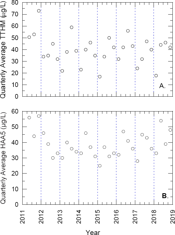
in the finished water, and it is highly likely that this ammonia would cause other, more severe and more immediate water quality problems, especially in light of the numerous rooftop water storage units throughout the NYC distribution system. These problems could include biofilm growth, nitrification (production of nitrite and then nitrate), and cause a loss of chlorine residual both in the distribution system and in these rooftop water storage units. With long detention times and low velocities in the storage vessels, the biological growth could become substantial and cause water quality problems; nitrifying bacteria are nonpathogenic, but they can secrete organic carbon products that can lead to yet more biological growth.
The primary source of NOM in the WOH reservoirs is the forest land that represent a significant fraction of the watershed area. Additional NOM sources are related to animal waste (e.g., cattle manure) and human waste (e.g., septic system discharge). In general, NOM sources are not easy to control, and that is true in the NYC watershed as well. Catastrophic events such as a large flood or an extensive forest fire could cause a nearly instantaneous and large spike in the NOM concentration, and such an event could trigger excessive DBP concentrations; note that the annual pattern of DBPs was different after Tropical Storms Irene and Lee compared to later periods. Over the long term, climate-induced changes in forest composition or annual snowmelt could well change the amount and the chemical structure of the NOM in the watershed, thereby affecting the amount and type of DBPs formed. Performing a careful analysis of the extensive monitoring data for DOM on a regular basis (every few years) is recommended so that NYC DEP might be able to anticipate regulatory troubles with DBPs. To the extent that NOM can be controlled, it would fall primarily under the purview of the Watershed Forestry Program, and secondarily on the Watershed Agricultural Program (to control animal manure) and the Septic System Program (to control human waste). Decreasing nutrient flux to the reservoirs (thereby controlling eutrophication) will indirectly help control NOM concentrations.
Microbial Pathogens
Pathogenic microorganisms (bacteria, viruses, and protozoa) originating from various sources can affect surface water supplies such as the NYC reservoirs. Waterborne pathogens emanate from both human (wastewater) and nonhuman sources (such as wildlife and livestock). Hence, the control of wastewater via upgrades to wastewater treatment plants and repair/replacement of septic systems, along with the Watershed Agricultural Program to control animal wastes, have been central to the Watershed Protection Program.
Indicators of potential pathogen contamination, including total and fecal coliforms, are routinely monitored at various points in the NYC water supply system. As discussed in Chapter 3, the SWTR requires that source water from unfiltered water supplies, sampled prior to disinfection, must have fecal coliform concentrations less than 20 CFU/100 mL (or total coliforms <100 CFU/100 mL) in at least 90 percent of samples. As shown in Figure 4-15, at no time in the last 20 years has the NYC DEP been out of compliance with the fecal coliform requirements of the SWTR, as measured in Kensico Reservoir at DEL18.
NRC (2000a) characterized the protozoan pathogens Giardia and Cryptosporidium as significant threats to the water supply due to their resistance to chlorine disinfection. That Committee’s analysis of pathogen monitoring data revealed that the daily risk of Cryptosporidium infection was higher than the EPA’s acceptable risk level for microbially caused illnesses. At that time, it was also known that about 7 percent of both wildlife and cattle in the NYC watershed were infected with Giardia (NYS WRI, 1997), although much lower percentages of cattle and wildlife were shown to be infected with C. parvum. The risk of cryptosporidiosis from drinking water was fresh in reviewers’ memories after the 1993 Milwaukee outbreak, and antiviral treatments were only beginning to reduce the risk to immune-compromised individuals with HIV8 (Fox and Lytle, 1996).
Since that time, a number of changes both locally within the NYC system and more broadly, have reduced the risk from Cryptosporidium. The longer record of testing within the watershed and at key points within the transmission system indicates that levels of Cryptosporidium are lower now than earlier, as shown in Figure 4-16. Testing procedures used by NYC DEP for Cryptosporidium have advanced, allowing identification of specific species: results generally indicate that the type of Cryptosporidium detected is unlikely to be infectious
___________________
8 See https://www.niaid.nih.gov/diseases-conditions/antiretroviral-drug-development.
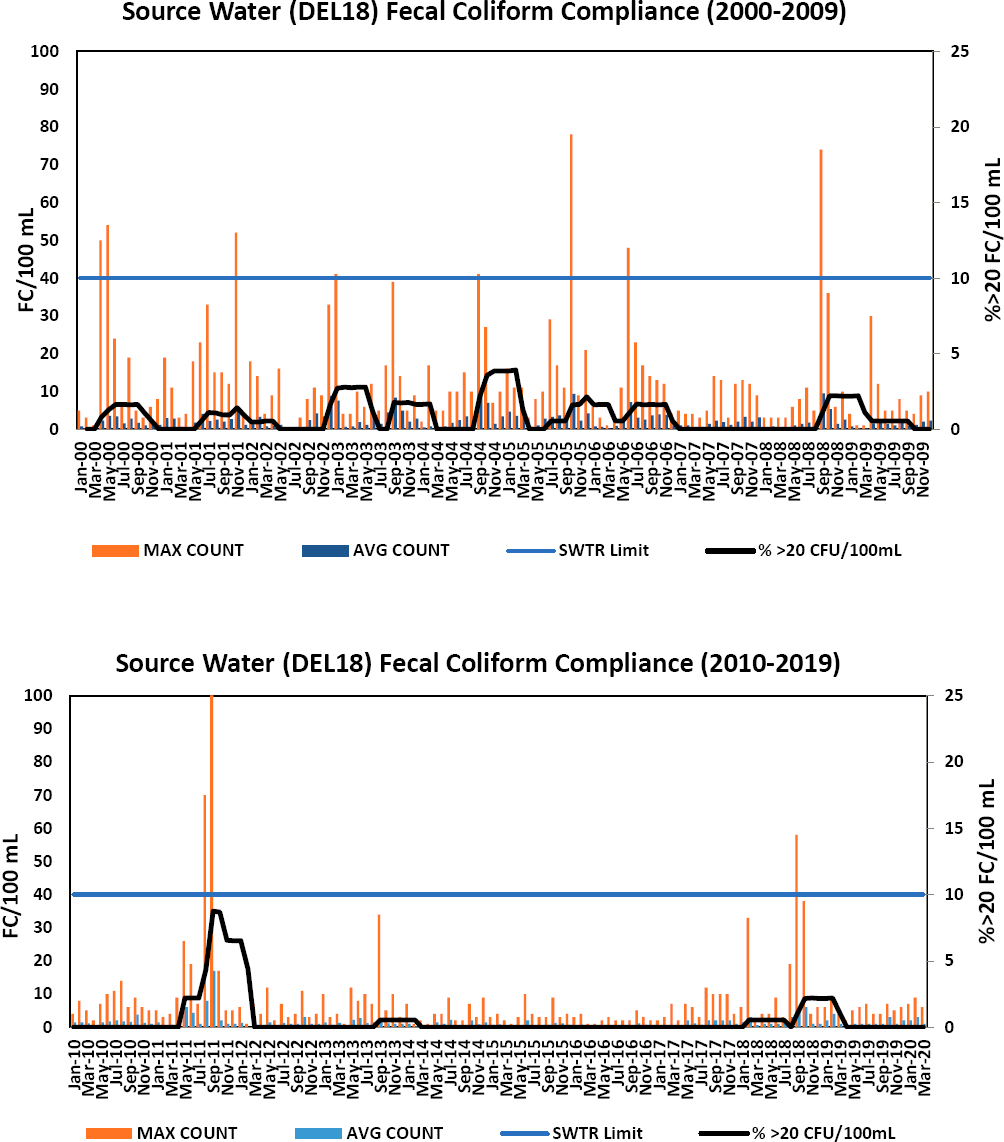
to humans (see Figure 4-17). Second, an important potential source of human infectious Cryptosporidium in the watershed—wastewater treatment plants—has been eliminated by NYC DEP’s substantial investment in advanced wastewater treatment at both its own and community treatment plants. Use of membrane filtration and UV disinfection allows removal and inactivation of potential pathogens from those waste streams. Finally, NYC DEP constructed and is now operating the UV facility, which was designed and is operated to reliably achieve a minimum of 99 percent inactivation of any infectious Cryptosporidium in the water, in contrast to the previous use of chlorine alone which was incapable of any Cryptosporidium inactivation (NYC DEP, 2016b). Results from infectivity studies on detected Cryptosporidium oocysts downstream of the UV plant at Hillview Reservoir appear to support the conclusion of substantial inactivation (Alderisio, 2018).
Need for a Mass Balance Approach
The Committee notes that much of the analysis reported by NYC DEP regarding the stressors discussed above are stated in terms of concentrations. This is understandable in that the regulations under which they operate typically express limits in those terms. However, in attempting to prioritize future water quality management actions, it is increasingly important to develop analyses that are based on mass balance (flux) of the various constituents of concern. The evaluation of strategies needs to be able to consider the inputs of constituents from point sources compared with the inputs from nonpoint sources and to assess the extent to which reductions in either or both of these sources will reduce the mass of the constituents in the reservoirs. If climate change results in changes in storm intensities and streamflow (as it is expected to) then the change in inputs to the reservoirs cannot be determined from concentration estimates alone. They can only come from multiplying concentrations times discharge rates to determine a constituent flux. The mass balance approach is described in more detail in Box 4-1.
There are several analytical strategies that can be used in such mass balance computations. The SPARROW (Spatially Reference Regressions on Watershed Attributes) model (Smith et al., 1997) is one formulation that has been effective in a number of regional water quality analyses; it is described and applied to the NYC watersheds in Chapter 12. Such formulations are crucial to identifying the relative importance of source types and relative importance of various subwatersheds in terms of controlling the total inputs of a pollutant. Predicting the future stressors of water quality depends on having (1) good data, (2) a system for tracking changing inputs (e.g., nutrients in the form of fertilizer, manure, atmospheric deposition, or point-source discharges), and (3) a system for using the available data to estimate the transformations of these inputs as they move downstream in the watershed system. Having such a mass-balance modeling approach is crucial to projecting the future of the system’s stressors as inputs change, as mitigation measures change, as land use changes, and as the climate changes.
THREATS ASSOCIATED WITH CLIMATE CHANGE
The frequency or magnitude of any of the threats described in this chapter can be expected to change as a result of the ongoing and future changes in climate. This report takes note of some of the ways that climate change can result in changing the nature and extent of these identified threats. The climate drivers that can be expected to change in the coming decades include precipitation amounts and intensities, precipitation type (snow versus rain), and air temperature. The topic of climate change for the NYC watershed region was considered in detail in the recent National Academies’ study of the OST (NASEM, 2018), which concluded that the NYC “water resources have been and will be affected significantly by climate change.” But the report goes on to say that “there continue to be … large uncertainties about the effects and their direction (wetter vs. drier), magnitude, duration, and seasonal timing.” Readers interested in the issue of climate change and its implications for the NYC water supply are encouraged to read Chapter 5 of that report.
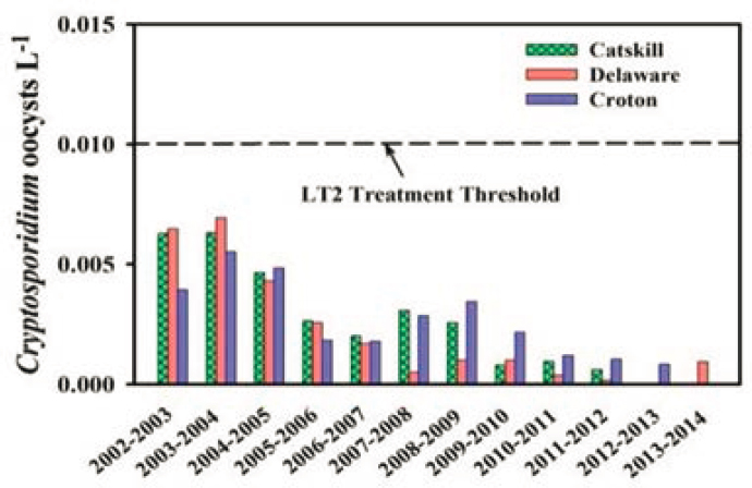
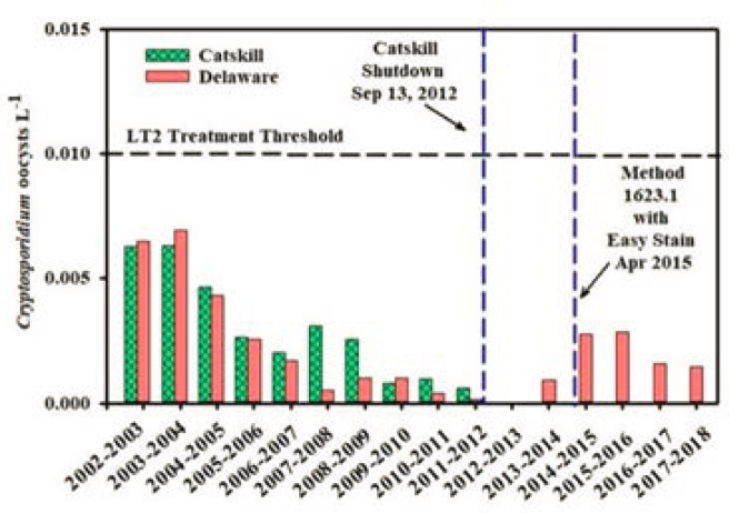
The National Climate Assessment (USGCRP, 2017) also explored the recent trends in climate and likely future trends highly relevant to the NYC watershed. Key findings that are most germane to NYC watershed protection are summarized here:
- Annual average air temperatures have been increasing nationwide, with an average increase of about 1.0°C for the period 1895–2016.
- Annual average air temperatures are projected to rise in the future, with a projected 1.4°C increase projected for the period 2021–2050 compared to 1976–2005.
- Annual precipitation has been increasing in the Northeast United States.
- Heavy precipitation events have increased in both intensity and frequency nationwide, and this trend will likely continue. The largest increases have occurred in the Northeast United States.
- Spring snow cover extent and snow depths have declined over all regions of the United States where snow is common, while at the same time extreme snowfall years have increased.
The National Climate Assessment uses a very specific set of terminology to express the degree of confidence about its findings. As a broad generalization, what one sees in reviewing the many findings that may relate to the NYC water supply is that findings related to temperature are generally considered to be high or very high confidence while those related to precipitation and flooding are typically of medium confidence. Water-related variables tend to be much more variable in time and space and exhibit a high degree of persistence. These characteristics make statistical analysis of them much more challenging than the analysis of temperature data. Also, the atmospheric processes that drive precipitation are difficult to simulate well in global climate models. As such, understanding the past changes and projecting future changes in indicators important to NYC watershed operations and protection will continue to be challenging, and results will have a high degree of uncertainty. NYC DEP will need to stay abreast of the developing knowledge of climate change and sharpen its own analytical skills to try to describe and understand the climate change signals of importance to its watershed. This theme is revisited in Chapter 12, Understanding the Watershed: Monitoring, Modeling and Assessment.
Finally, the New York City Panel on Climate Change report (NPCC, 2019) provides an excellent basis for learning about some of the climate trends to date in the New York City region and expected trends in the future. The following sections discuss aspects of climate change and their possible linkage to water quality impacts in the New York City watershed. How climate change may affect specific subprograms of the Watershed Protection Program is discussed in Chapters 5 through 11.
Changes in the Magnitude and Frequency of Extreme Precipitation Events and Associated Runoff
Chapter 2 of the New York City Panel on Climate Change report (González et al., 2019) describes some recent increases and projections of future increases in “heavy downpours” in the New York City watershed region, but notes that the projections have a higher degree of uncertainty than temperature projections. Increased frequency and/or magnitude of heavy downpours and the streamflow that is generated by these events is very likely to bring about increases in the magnitude and duration of high-turbidity events. The nonlinear nature of the relationship between stream discharge and turbidity levels (as depicted in the right panel of Figure 4-7) could mean that a small percentage change in precipitation or streamflow will result in large percentage increases in turbidity in the absence of turbidity control measures. This possibility highlights the importance of the streambank restoration efforts taking place in the watershed (see Chapter 6). Continued monitoring and data analysis for precipitation event size, peak streamflow discharges, and turbidity levels in streams should be a high priority for NYC DEP.
The impact of higher precipitation intensities on nitrogen and phosphorus is much less clear. Certainly changes in rainfall intensity in large precipitation events would change the timing of transport of nitrogen and phosphorus, with more of it moving in these large events. However, the total amounts of nitrogen and phosphorus lost from the landscape and transported downstream will not necessarily change. The total losses of nitrogen and phosphorus from the landscape are largely controlled by the rate at which nitrogen and phosphorus are applied to the land surface from their main sources: chemical fertilizer application, manure application, septic tank losses to soil and groundwater, and atmospheric deposition. In other words, if large storms become more intense over time, the amount of nitrogen or phosphorus transported off the landscape during these events would likely increase, but decreases in transport during smaller events or low flows may largely cancel out these increases because the average rate of transport is mostly controlled by their availability. The concerns
with nutrients in the NYC watershed are related to the potential for eutrophication of the reservoirs and this process is influenced by average loading rates (averaged over a few months or an entire year) as opposed to being driven by peak loading rates during an event. Analyses of stream nutrient trends need to focus on average loads at a seasonal to annual time scale and not on concentrations (although concentration measurements and discharge measurements are vital to the analysis).
Stream Flow
The analyses of stream nutrient loads carried out in the future by NYC DEP must be done in a manner that recognizes the importance of the streamflow changes that have already taken place. NASEM (2018) described the observed trends at a set of seven stream gages in the watershed (all located above NYC reservoirs). That analysis shows very large (and in many cases statistically significant) upward trends. The summer and fall one-day maximum streamflow showed upward trends at all of these stream gages over the period 1951–2017, with summer trends ranging from 135 up to 3079 percent of the initial values. The fall trends were smaller (68 to 116 percent) but not statistically significant. Trends in mean daily streamflow at these same stream gages followed a similar pattern but with a smaller magnitude. Summer discharge values increased from 100 to 155 percent across the set of seven stream gages (all were statistically significant). Fall and winter streamflows all showed upward trends, from 14 to 88 percent, but most of these were not statistically significant. Spring streamflows showed modest decreases of -5 to -20 percent (only one of these was significant).
A previous study of streamflow in Catskill region watersheds (Burns et al., 2007), focusing on the period 1952–2005, showed increases at all of the sites studied but none were significant. Only with the addition of the 12 years (2006–2017) did they become significant. Burns et al. (2007) also found that streamflow trends were positive in all months except for February and April. The April decrease was very substantial, probably signifying the fact that in recent years snowmelt has come earlier, resulting in higher March flows and lower April flows. All of these results indicate that streamflow trends are not simply something anticipated in the future, but rather are a regionwide condition that has been under way for a few decades.
The analysis reported earlier in this chapter, on phosphorus inputs to Cannonsville Reservoir, illustrates why considering climate change can be important to the analysis of water quality change. In this case, trends in the flux of TP from 1988 to 2018 showed an increase of 88 percent. If the trends in streamflow over this period had been ignored, the increase would have been estimated to be 51 percent. Failure to consider streamflow trends can result in serious errors in estimation of loading trends. The effectiveness of certain BMPs in the watershed, such as retention basins, will depend in part on streamflow trends, which are largely climate driven.
It is likely that increased runoff will exacerbate the problems with microbial pathogen loading already caused by nonpoint sources such as manure application, failing septic systems, and sewer overflows. Sterk et al. (2013) found that norovirus contaminated surface water via the increased sewage discharge that accompanied heavy rainfall events. A similar effect may occur with improperly sited or constructed septic systems. The increases in nutrient loading brought about by increased stream flows could also enhance the abundance and survival of pathogens that thrive in eutrophic reservoirs (Smith and Schindler, 2009).
Extreme Events
Trends in the most extreme precipitation and discharge conditions are very difficult to evaluate, both because they are so infrequent and because of the strong tendency towards persistence (periods of several years with many extreme events followed by periods of several years largely devoid of such events). Figure 4-18 provides an example of such a record at one of the longest record stream gages in the watershed, Schoharie Creek
___________________
9 A 307 percent increase indicates that one-day maximum streamflow values at the end of this period were more than 4 times the magnitude of one-day maximum streamflow values, based on the general trend observed over the full 67-year record. The smallest of the increases, 135 percent, represents more than a doubling over the 67 years.
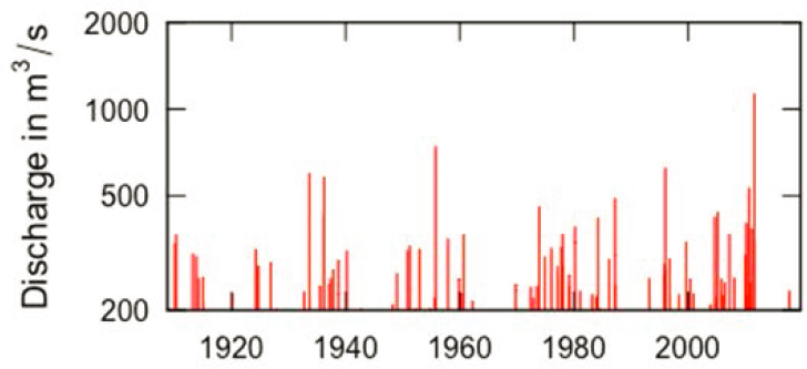
at Prattsville, New York. It shows discharge values only on those days that exceeded a threshold of 200 m3/s. This is a discharge that is has been exceeded, on average, about 1 day per year and is approximately 14 times the long-term mean discharge. The record shows the high degree of persistence in the extreme flow record, with the time period around 2011 being one of frequent and large extremes, but in contrast, the period 2012–2019 has been nearly devoid of such events. Analyses of records of the frequency and magnitude of discharges above various high thresholds is crucial to evaluation of high-turbidity threats. Unlike nitrogen and phosphorus, the issue of greatest concern for turbidity are these very high streamflow events and the short-term high turbidity associated with them. The supply of fine-grained sediments in the bed and banks of the streams is virtually infinite in the areas of high-source turbidity such as Upper Esopus Creek. Thus, any tendency toward an increase in the frequency or magnitude of these very high events presents an added challenge to the turbidity control problem.
Changes in Ice Cover Duration on the New York City Reservoirs
As discussed previously in this chapter, the duration of the ice-free period appears to be an important factor in the development of HABs. Ice cover and cold temperatures inhibit photosynthetic activity. As such, when the ice melts photosynthesis activity can rapidly increase leading to the growth of various algal species (including Cyanobacter). Also, earlier ice breakup facilitates an earlier initiation of thermal stratification. Thermal stratification can contribute to both eutrophication and HABs because the low-oxygen conditions near the reservoir bed can lead to increased mobility of the phosphorus stored in the bed sediments. Analyses of threats, particularly of HABs, should include a long-term analysis of water temperatures in the reservoirs and dates of ice formation and ice breakup. These physical factors can be important drivers of this biotic condition. A summary of lake ice data from North America and Europe (Benson et al., 2012) found that, over the period from the winter of 1975-1976 to 2004-2005, the mean date of ice breakup over the lakes studied became earlier in the year by a rate of -1.87 days/decade. The Committee encourages NYC DEP to explore the history of ice breakup timing and also lake temperature for their system of reservoirs and conduct some analyses to see how ice cover statistics and lake temperature have been changing over time.
Changes in Snowpack and Frozen Soil Conditions
The change in climate that has taken place in recent decades has resulted in a change in the timing of snowmelt runoff. Burns et al. (2007) estimated that the change in the winter-spring center of volume has been
about two to eight days earlier per 50 years (based on the 1952–2005 discharge records at eight Catskill region streams). This shift in the timing of runoff is expected to continue into the coming decades and will need to be incorporated into OST. It is likely that winter rain may become more common while winter snow becomes less common.
It is not clear what the implications of these changes may be for water quality. Snowpack conditions and the timing and extent of frozen ground can be relevant to various types of nonpoint source pollution, in particular pollution associated with manure application. Manure management approaches, particularly in the winter, will need to adjust to this new reality. NYC DEP and the Watershed Agricultural Council should be exploring these trends and modifying guidance to farmers to adjust to these changes. With a longer period of generally wet, but not frozen, soil conditions in the late winter and early spring, the natural microbial processing of the organic matter in the soil can be expected to result in changes in the amount and types of NOM transported down the rivers to the reservoirs. This may have an impact on the production of compounds that can produce DBPs in the finished water supply.
Changes in Air Temperatures and Resulting Impacts on Water Temperatures
Increasing air temperatures are of particular importance to NYC watershed protection because of their influence on water temperatures in the streams and reservoirs of the NYC system. The rates of many biological and chemical processes in aquatic ecosystems increase with water temperature. Also, the saturation concentration of dissolved oxygen decreases with increasing water temperature. This means that warmer temperatures can increase the potential for low dissolved oxygen conditions in the reservoirs and concomitant release of phosphorus from reservoir sediments into the water column. Thus, high water temperature could lead to increases in the potential for eutrophication and HABs.
It is unclear whether increased water temperatures will increase or decrease rates of waterborne disease. For example, Britton et al. (2010) found a positive association of giardiasis with temperature and rainfall; however, cryptosporidiosis was positively associated with rainfall but negatively impacted by temperature. The survival of Cryptosporidium oocysts in a variety of media has been shown to decrease with temperature (reviewed in Peng et al., 2008). However, differentiating the direct effects of temperature on microorganism survival from other, more indirect effects of climate change, such as changes in the timing and amount of runoff, has not occurred in most studies, making conclusions tenuous. For example, increases in water temperature or precipitation, as well as drought conditions, were found to indirectly influence the persistence and spread of cholera bacteria by increasing the concentration of the vectors (e.g., copepods) that carry the bacteria (Cottingham et al., 2003; Smith and Schindler, 2009). Sterk et al. (2013) showed that higher temperatures and an increase in precipitation, nutrients, and salinity due to heavier rain events can enhance pathogen growth, survival, replication, and mobilization and may lead to increased rates of waterborne disease. Even extreme drought conditions can indirectly affect pathogen loading by concentrating pathogens in limited water supplies (Levy et al., 2016).
***
In summary, the ongoing and future changes in climate will present challenges to the Watershed Protection Program specifically and operation of the NYC water supply in general. The Committee does not believe that any of these climate-driven threats make filtration of the water supply necessary in order to provide adequate water quality protection. However, climate change heightens the importance of an adaptive management approach to municipal water supply (see Chapter 1). Rosenzweig and Solecki (2019) describe an adaptive management approach for a variety of time scales in the introduction to the New York City Panel on Climate Change Report (NPCC, 2019). Their summary, also presented in graphical form (Figure 4-19) is applicable to any aspect of infrastructure management or services of a large urban system. Clearly, monitoring and assessment, awareness of the latest research findings, and modification of structural and operational aspects of the water supply system in response to emerging knowledge is essential.
NYC Water Supply Resiliency
At the request of the Committee, modelers at the NYC DEP ran several scenarios within the OST modeling platform to assess what size of storm event would cause the water supply to violate the SWTR criterion of five NTU at the outlet of Kensico Reservoir. This request was prompted largely by the difficult situation presented by Tropical Storms Irene and Lee in 2011, during which alum was used extensively to avoid violating the turbidity standard.
In creating the OST simulation, NYC DEP considered Irene and Lee to be a single event, and they then simulated the occurrence of two double events (i.e., Irene–Lee followed by Irene–Lee). The double events were separated by a week and assumed to occur on September 6–8, and then on September 15–28, resulting in a prolonged threat to complying with the turbidity standard. Using the observed hydrology after Irene, the model assumed a continuous type of hydrology over the two double events. This is a far worse set of storm conditions than has ever been observed historically. The extreme storm events were applied to the entire WOH watershed.
OST was initialized with conditions prior to Irene. Stratification of compounds within the reservoirs was modeled with the water quality model CE-QUAL-W2 (W2, see Chapter 12 for a description). The same starting elevation was used in all the reservoirs. No operational decisions were predetermined. The Croton system was on for the entire run with filtration, and full water demand was assumed throughout all scenarios. Finally, water from the Catskill system was dosed with alum throughout all scenarios.
The results of the evaluation (NYC DEP, personal communication, July 2019) demonstrate the flexibility and robustness of the NYC water supply system to such extreme storm events, as well as the utility of OST (discussed in Chapter 12 and NASEM, 2018). A series of operational scenarios were evaluated; information from scenarios that did not meet the turbidity standard were used to design subsequent scenarios. In 11 of the 13 simulations, which all involved changing operations within the Delaware system, the turbidity criterion at
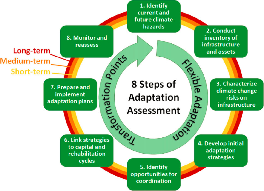
Kensico was violated but turbidity remained less than 6 NTU. However, when Rondout was removed from service (meaning no NYC water was delivered from the Delaware system), the simulations showed that Kensico Reservoir turbidity stayed below 5 NTU. During this time, water demand was met except on one day. However, the simulations suggested that it could take months for the turbidity to decrease following such an immense series of storms, implying long periods of alum addition and care. OST allowed NYC DEP managers to evaluate these scenarios, learning from and discarding ones that were inferior. Were such an event to occur, the OST modeling platform would allow NYC DEP staff to quickly evaluate multiple scenarios and suggest an operational solution.
The runs demonstrated the operational flexibility of the NYC water supply. Additional flexibility could be gained by adding alum treatment to Delaware system diversions. NYC DEP is developing W2 models for Pepacton, Cannonsville, and Neversink; the absence of W2 does present uncertainty in the simulations because the modelers had to assume the turbidity of water incoming from those three reservoirs. A wider range of such modeling stress tests might more systematically identify conditions where system operations become fragile or likely to fail, along with the consequences and promising management responses for likely failures.
This analysis supported three lessons. First, the NYC water supply system’s flexibility greatly reduces its vulnerability to very extreme events (far beyond historical events). Second, operational flexibility, bolstered by OST, provides a useful component to enhance the multiple barrier approach to water delivery. Finally, this type of stress test is useful for identifying problematic conditions so that they can be better prepared for and prioritized.
CONCLUSIONS AND RECOMMENDATIONS
The climate and hydrology of the Catskill Mountain region is highly variable, requiring vigilant and proactive operations of the water supply system by the New York City Department of Environmental Protection. This long-standing management paradigm has been severely tested by extreme conditions over more than a century of operations. These challenges will continue and may be amplified by global climate change. This underscores the critical importance of full and sustained support of the Water Supply Operations Center and core functions of the Bureau of Water Supply.
Land cover and land use changes from forest and farmland to developed areas in the west-of-Hudson watersheds have been minimal, one-tenth the average change for New York State, from 2001 to 2016. This stability can be attributed to the Memorandum of Agreement, Watershed Protection Program, forest and agricultural land conservation efforts, and recent market trends for agricultural and forest products.
Compared to 20 years ago, the constituents of greatest concern have shifted from microbial pathogens to turbidity, phosphorus, and natural organic matter. Turbidity is a top-priority pollutant for the NYC water supply for the foreseeable future because of (1) the low-turbidity target for regulatory compliance, (2) the nature of the sources of turbidity in the Catskill system, and (3) the uncertainty about how restored stream corridors will perform during extreme events. Phosphorus, and more generally, nutrients, are the second priority, given the associated risks of hazardous algal blooms contributing to direct toxicity, turbidity problems, and anoxic conditions in the reservoirs. NOM is the third priority due to the creation of DBPs. Finally, due to UV disinfection, which treats all of the water that passes into the distribution system, microbial pathogens are a lesser, but still important, concern. For the highest priority pollutants, adopting a mass-balance modeling approach is crucial to understanding their future role as system stressors under changing conditions (e.g., climate, land use, and implementation of mitigation measures).
The Committee’s mass-balance analysis of phosphorus data shows that total phosphorus flux trends for the West Branch of the Delaware River above Cannonsville Reservoir are moving in the right direction since 2010, but the rate of improvement is very slow. NYC DEP should be exploring
potential explanations for the period of steep increases in flow-normalized flux (2000-2010) as well as the reasons why the most recent decade is relatively trend-free. Understanding the reasons for temporal patterns of phosphorus inputs to Cannonsville Reservoir and phosphorus concentrations in the reservoir is crucial to developing strategies to prevent eutrophic conditions and the development of harmful algal blooms.
Predicted changes to climate in the New York City watershed region are likely to have several undesirable effects on reservoir water quality from increased nonpoint source pollution. Climate change will likely lead to an increased intensity of storm events, thereby exacerbating turbidity loading problems. The concentration and characteristics of NOM in the reservoirs may change, increasing concentrations of DBPs or extending periods when the highest DBP concentrations are formed. NYC DEP should regularly analyze their monitoring data for trends that would identify such changes and indicate whether water quality parameters could be altered by climate change.
New York City’s Watershed Protection Program and system operations appear able to more than adequately protect the quality of the city’s drinking water source, even under extraordinary storm conditions. Modeling studies show that even when subjected to events much greater than historical extremes, water quality failures defined by exceedance of the 5 NTU turbidity standard at Kensico would be rare and small (less than 6 NTU) if properly managed. Turning to filtration to protect against the water quality impact of extreme events do not appear warranted at this time. Retrospective performance analyses should follow major potential contamination events and rigorous, systematic assessments (“stress tests”) should occur at least every five years. Such assessments can identify operational and infrastructure vulnerabilities for further consideration.
REFERENCES
Alderisio, K. A. 2018. Protozoan Monitoring and Analysis at Hillview Reservoir. Presentation at Meeting 2 of the NASEM Committee to Review the NYC DEP Watershed Protection Program. Rhinebeck, NY. October 24-26.
Auer, M. T., K. A. Tomasoski, M. J. Babiera, M. Needham, S. W. Effler, E. M. Owens and J. M. Hansen. 1998. Phosphorus bioavailability and P-cycling in Cannonsville Reservoir. Lake and Reservoir Management 14(2-3):278-289.
Benson, B. J., Magnuson, J. J., Jensen, O. P., Card, V. M., Hodgkins, G., Korhonen, J., Livingstone, D. M., Stewart, K. M., Weyhenmeyer, G. A. and Granin, N. G. 2012. Extreme events, trends, and variability in northern hemisphere lake-ice phenology (1855–2005). Climatic Change 112(2):299-323.
Boström, B., J. M. Andersen, S. Fleischer, and M. Jansson. 1988. Exchange of phosphorus across the sediment-water interface. Pp. 229-244 In: Phosphorus in freshwater ecosystems. Dordrecht, the Netherlands: Springer.
Britton, E., Hales, S., Venugopal, K., and Baker, M. G. 2010. The impact of climate variability and change on cryptosporidiosis and giardiasis rates in New Zealand. Journal of Water and Health 8(3):561-571.
Brooks, K. N., P. F. Ffolliott, and J. A. Magner. 2013. Hydrology and the Management of Watersheds. 4th Edition. Ames, IA: Wiley-Blackwell.
Burns, D. A., J. Klaus, and M. R. McHale. 2007. Recent climate trends and implications for water resources in the Catskill Mountain Region, New York, USA. Journal of Hydrology 336(1-2):155-170.
Carlson, R. E. 1977. A trophic state index for lakes. Limnology and Oceanography 22:361-369.
Choquette, A. F., R. M. Hirsch, J. C. Murphy, L. T. Johnson, and R. B. Confesor, Jr. 2019. Tracking changes in nutrient delivery to Western Lake Erie: Approaches to compensate for variability and trends in streamflow. Journal of Great Lakes Research 45(1):21-39.
Cottingham, K. L., D. A. Chiavelli, and R. K. Taylor. 2003. Environmental microbe and human pathogen: The ecology and microbiology of Vibrio cholerae. Frontiers in Ecology and the Environment 1(2):80-86.
de la Crétaz, A. L., and P. K. Barten. 2007. Land Use Effects on Streamflow and Water Quality in the Northeastern United States. Boca Raton, Florida and London: CRC Press.
Doerr, S. M., E. M. Owens, R. K. Gelda, M. T. Auer, and S. W. Effler. 1998. Development and testing of a nutrient-phytoplankton model for Cannonsville Reservoir. Lake and Reservoir Management 14(2-3):301-321.
Effler, S. W., M. G. Perkins, N. Ohrazda, C. M. Brooks, B. A. Wagner, D. L. Johnson, F. Peng and A. Bennett. 1998. Turbidity and particle signatures imparted by runoff events in Ashokan Reservoir, NY. Lake and Reservoir Management 14(2-3):254-265.
Foster, D., K. Fallon Lambert, D. Kittredge, B. Donahue, C. Hart, William. Labich, S. Meyer, J. Thompson, M. Buchanan, J. Levitt, R. Perschel, K. Ross, G. Elkins, C. Daigle, B. Hall, E. Faison, A. D’Amato, R. Forman, P. Del Tredici, L. Irland, B. Colburn, D. Orwig, J. Aber, A. Berger, C. Driscoll, W. Keeton, R. Lilieholm, N. Pederson, A. Ellison, M. Hunter, and T. Fahey. 2017. Wildlands and Woodlands: Farmlands and Communities—Broadening the Vision for New England. Harvard Forest, Petersham, MA. https://www.wildlandsandwoodlands.org/sites/default/files/Wildlands%20and%20Woodlands%202017%20Report.pdf.
Fox, K. R., and D. A. Lytle. 1996. Milwaukee’s crypto outbreak: Investigation and recommendations. Journal of the American Water Works Association 88(9):87-94.
Gergel, S. E., M. G. Turner, J. R. Miller, J. M. Melack, and E. H. Stanley. 2002. Landscape indicators of human impacts to riverine systems. Aquatic Sciences 64(2):118-128.
González, J. E., L. Ortiz, B. K. Smith, N. Devineni, B. Colle, J. F. Booth, A. Ravindranath, L. Rivera, R. Horton, K. Towey, and Y. Kushnir. 2019. New York City Panel on Climate Change 2019 Report. Chapter 2: New Methods for Assessing Extreme Temperatures, Heavy Downpours, and Drought. Annals of the New York Academy of Sciences 1439:30-70.
Hamon, W. R. 1961. Estimating potential evapotranspiration. Journal of the Hydraulics Division of the American Society of Civil Engineers 87:107-120.
Hirsch, R. M., D. L. Moyer, and S. A. Archfield. 2010. Weighted regressions on time, discharge, and season (WRTDS), with an Application to Chesapeake Bay river inputs. Journal of the American Water Resources Association 46(5):857-880.
Hirsch, R. M., S. A. Archfield, and L. A. De Cicco. 2015. A bootstrap method for estimating uncertainty of water quality trends. Environmental Modelling & Software 73:148–66.
Homer, C., J. Dewitz, S. Jin, G. Xian, C. Costello, P. Danielson, L. Gass, M. Funk, J. Wickham, S. Stehman, R. Auch, and K. Riitters. 2020. Conterminous United States land cover change patterns 2001-2016 from the 2016 National Land Cover Database. ISPRS Journal of Photogrammetry and Remote Sensing 162(2020):184-199.
Huisman, J., G. A. Codd, H. W. Paerl, B. W. Ibelings, J. M. H. Verspagen, and P. M. Visser. 2018. Cyanobacterial Blooms. Nature Reviews Microbiology 16(8):471.
Johnson, L., C. Richards, G. Host, and J. Arthur. 1997. Landscape influences on water chemistry in Midwestern stream ecosystems. Freshwater Biology 37(1):193-208.
Levy, K., A. P. Woster, R. S. Goldstein, and E. J. Carlton. 2016. Untangling the impacts of climate change on waterborne diseases: A systematic review of relationships between diarrheal diseases and temperature, rainfall, flooding, and drought. Environmental Science and Technology 50(10):4905-4922.
Livengood, K. 2016. Extracting Harvest Sites from Imagery. Forestry Source 21(6):16-17.
McHale, M. R., and J. Siemion. 2014. Turbidity and Suspended Sediment in the Upper Esopus Creek Watershed, Ulster County, New York. U.S. Geological Survey Scientific Investigations Report, 2014-5200. https://pubs.usgs.gov/sir/2014/5200/pdf/sir2014-5200.pdf.
Mukundan, R. 2019. Watershed Modeling. Presentation at Meeting 3 of NASEM Committee to Review the NYC DEP Watershed Protection Program. West Harrison, NY. February 4.
NASEM (National Academies of Sciences, Engineering, and Medicine). 2018. Review of the New York City Department of Environmental Protection Operations Support Tool for Water Supply. Washington, DC: The National Academies Press.
National Research Council (NRC). 2000a. Watershed Management for Potable Water Supply: Assessing the New York City strategy. Washington, DC: The National Academies Press.
NRC. 2000b. Clean Coastal Waters: Understanding and Reducing the Effects of Nutrient Pollution. Washington, DC: The National Academies Press.
NRC. 2008. Hydrologic Effects of a Changing Forest Landscape. Washington, DC: The National Academies Press.
Niyogi, D. K., K. S. Simon, and C. R. Townsend. 2004. Land use and stream ecosystem functioning: nutrient uptake in streams that contrast in agricultural development. Archiv für Hydrobiologie 160(4):471-486.
NPCC (New York City Panel on Climate Change). 2019. Advancing Tools and Methods for Flexible Adaptation Pathways and Science Policy Integration: New York City Panel on Climate Change 2019 Report. C. Rosenzweig and W. Solecki (eds.). Annals of the New York Academy of Sciences 1439:1–311.
NYC DEP. 1999. Development of a Water Quality Guidance Value for Phase II Total Maximum Daily Loads (TMDLs) in the New York City Reservoirs. Valhalla, NY: NYC DEP.
NYC DEP. 2008. Catskill Turbidity Control Study Phase III Final Report. Valhalla, New York: NYC DEP.
NYC DEP. 2013. New York City 2013 Drinking Water Supply and Quality Report.
NYC DEP. 2014. New York City 2014 Drinking Water Supply and Quality Report.
NYC DEP. 2015. New York City 2015 Drinking Water Supply and Quality Report. https://www.yorktownny.org/sites/default/files/fileattachments/general/page/4142/2015_nyc_water_supply_quality_report.pdf.
NYC DEP. 2016a. New York City 2016 Drinking Water Supply and Quality Report. https://smartnet.niua.org/sites/default/files/resources/wsstate16.pdf.
NYC DEP. 2016b. Watershed Protection Plan Summary and Assessment, March 2016.
NYC DEP. 2017. New York City 2017 Drinking Water Supply and Quality Report. https://www1.nyc.gov/assets/nyw/downloads/pdf/nyw-2017-dep-water-report.pdf.
NYC DEP. 2018a. 2017 Watershed Water Quality Annual Report.
NYC DEP. 2018b. New York City 2018 Drinking Water Supply and Quality Report. https://www1.nyc.gov/assets/dep/downloads/pdf/water/drinking-water/drinking-water-supply-quality-report/2018-drinking-water-supply-quality-report.pdf.
NYC DEP. 2019. New York City 2019 Drinking Water Supply and Quality Report. https://www1.nyc.gov/assets/dep/downloads/pdf/water/drinking-water/drinking-water-supply-quality-report/2019-drinking-water-supply-quality-report.pdf.
NYS DEC. 2017. Final Scope for the Modification of the CATALUM SPDES Permit Environmental Impact Statement. Lead Agency: New York State Department of Environmental Conservation. Applicant: New York City Department of Environmental Protection. March.
NYS WRI (New York State Water Resources Institute). 1997. Science for Whole Farm Planning: Cornell University Phase II Twelfth Quarter and Completion Report.
Nürnberg, G. K. 1994. Phosphorus release from anoxic sediments: What we know and how we can deal with it. Limnetica 10(1):1-4.
Paerl, H. W., and J. Huisman. 2008. Blooms like it hot. Science 320(5872): 57-58.
Paerl, H. W., K. E. Havens, N. S. Hall, T. G. Otten, M. Zhu, H. Xu, G. Zhu, and B. Qin. 2019. Mitigating a global expansion of toxic cyanobacterial blooms: Confounding effects and challenges posed by climate change. Marine and Freshwater Research 71:579-592.
Peng, F., D. L. Johnson, and S. W. Effler. 2002. Suspensoids in New York City’s drinking water reservoirs: Turbidity apportionment. Journal of the American Water Resources Association 38(5):1453-1465.
Peng, F., D. L. Johnson, and S. W. Effler. 2004. Characterization of inorganic particles in selected reservoirs and tributaries of the New York City Water Supply. Journal of the American Water Resources Association 40(3):663-676.
Peng, X., T. Murphy, and N. M. Holden. 2008. Evaluation of the effect of temperature on the die-off rate for Cryptosporidium parvum Oocysts in water, soils, and feces. Applied and Environmental Microbiology 74(23):7101-7107.
Rabalais, N. N., R. E. Turner, and W. J. Wiseman Jr. 2002. Gulf of Mexico Hypoxia, aka “The Dead Zone.” Annual Review of Ecology and Systematics 33(1):235-263.
Reckhow, D. A., and P. C. Singer. 2011. Formation and control of disinfection by-products. In: Water Quality and Treatment: A Handbook on Drinking Water. 6th ed. New York: McGraw-Hill, American Water Works Association.
Richards, C., L. B. Johnson, and G. E. Host. 1996. Landscape-scale influences on stream habitats and biota. Canadian Journal of Fisheries and Aquatic Sciences 53(S1):295-311.
Rosenzweig, C., and W. Solecki. 2019. Pp. 22-29 In: Advancing Tools and Methods for Flexible Adaptation Pathways and Science Policy Integration: New York City Panel on Climate Change 2019 Report. Annals of the New York Academy of Sciences 1439:1–311.
Sharpley, A., H. P. Jarvie, A. Buda, L. May, B. Spears, and P. Kleinman. 2013. Phosphorus legacy: overcoming the effects of past management practices to mitigate future water quality impairment. Journal of Environmental Quality 42(5):1308-1326.
Smith, R. A., G. E. Schwarz, and R. B. Alexander. 1997. Regional interpretation of water-quality monitoring data. Water Resources Research 33(12). https://doi.org/10.1029/97WR02171.
Smith, D. R., M. L. Macrae, P. J. A. Kleinman, H. P. Jarvie, K. W. King, and R. B. Bryant. 2019. The latitudes, attitudes, and platitudes of watershed phosphorus management in North America. Journal of Environmental Quality 48(5):1176-1190.
Smith, V. H., and D. W. Schindler. 2009. Eutrophication science: where do we go from here? Trends in Ecology and Evolution 24:201–207.
Smol, J. P. 2019. Under the radar: Long-term perspectives on ecological changes in lakes. Proceedings of the Royal Society B 286(1906):20190834.
Sterk, A., J. Schijven, T. de Nijs, and A. M. de Roda Husman. 2013. Direct and indirect effects of climate change on the risk of infection by water-transmitted pathogens. Environmental Science and Technology 47(22):12648-12660.
Sweeney, B. W., T. L. Bott, J. K. Jackson, L. A. Kaplan, J. D. Newbold, L. J. Standley, W. C. Hession, and R. J. Horwitz. 2004. Riparian deforestation, stream narrowing, and loss of stream ecosystem services. Proceedings of the National Academy of Sciences 101(39):14132-14137.
USGCRP (U.S. Global Change Research Program). 2017. Climate Science Special Report: Fourth National Climate Assessment, Volume I. D. J. Wuebbles, D. W. Fahey, K. A. Hibbard, D. J. Dokken, B. C. Stewart, and T. K. Maycock (eds.). U.S. Global Change Research Program, Washington, DC. https://science2017.globalchange.gov/downloads/CSSR2017_FullReport.pdf.
USGS (U.S. Geological Survey). 2020. National Water Information System data available on the World Wide Web (USGS Water Data for the Nation). https://waterdata.usgs.gov/ny/nwis/dv/?site_no=01350000&agency_cd=USGS&.
VanBrakle, J., and T. Pavlesich. 2017. Assessing the BMP Program’s Reach Using Aerial Photographs and Arc-GIS. Watershed Agricultural Council, Walton, NY.


