
Appendix D
Bayesian Methods
This appendix presents an example of a Bayesian model that could be used by fishery managers to set season lengths and decide on season closure dates under an annual catch limit (ACL). The example presented here is a modified version of the Clark (1990) model. The example focuses on the management of a single-species fishery located in a particular geographic region, but the approach can be extended to multiple-species and/or multiple-region fisheries.
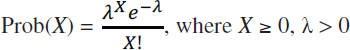
Consider a single-species fishery with an ACL that is set for the upcoming year by a stock assessment process. On any given fishing day, all anglers together in the fishery engage in a number, n, of fishing “attempts” (think of a fishing attempt as a single cast of a fishing line), each of which results in either a legally caught fish with average probability p or a failure with probability 1 – p. The binomial probability distribution gives the probability of X successes (i.e., X fish caught) in n fishing attempts. If the number of fishing attempts n is large, and the probability of success p on any individual fishing attempt is low, as would typically be the case, then the binomial probability distribution is well approximated by the Poisson distribution with parameter λ = n×p, where λ is the expected (mean) number of successes per time period (i.e., λ = the average daily total catch of all fishers together). The Poisson distribution is widely used to model the probability distribution of any discrete random variable arising from a binomial probability process (Ross, 2010). Hence, following Clark (1990), it is assumed that total fish catch per day, X, in the fishery follows a Poisson process with parameter λ:
Parameter λ is a random variable that may vary from season to season and indeed may vary within a season as the result of such factors as varying fishing effort (which may, in turn, depend on varying weather conditions and such economic factors as fuel costs and the unemployment rate), and varying catch per unit effort (which may, in turn, depend on such factors as varying stock sizes of legally harvestable fish [e.g., within size limits], varying gear types employed, and varying vessel size). Fishery managers do not know the precise value of λ on any particular day, but they can estimate the expected or mean value of λ, denoted μprior, and its variance, denoted ![]() , based
, based
on prior historical data, such as data from the Marine Recreational Information Program (MRIP). For example, MRIP Fishing Effort Survey data from the prior years could be used to estimate the mean and variance of the number of angler trips per day from the previous fishing season; MRIP Access Point Angler Intercept Survey data from the prior year could be used to estimate the mean and variance of catch per trip from the previous fishing season; and the two estimates could be combined to yield estimates of μprior and ![]() for mean (total for the fishery) catch per day, λ. If some other method were judged (by a Scientific Statistical Committee, for example) to yield better estimates of the mean and variance of λ, that alternative method could be used instead. For example, the mean and variance of λ could be estimated from a time series of MRIP data rather than data from only the prior year, or data from the previous 3 years, or the previous 5 years minus the highest and lowest years could be used. Any of these methods could be used to obtain the best estimates of μprior and
for mean (total for the fishery) catch per day, λ. If some other method were judged (by a Scientific Statistical Committee, for example) to yield better estimates of the mean and variance of λ, that alternative method could be used instead. For example, the mean and variance of λ could be estimated from a time series of MRIP data rather than data from only the prior year, or data from the previous 3 years, or the previous 5 years minus the highest and lowest years could be used. Any of these methods could be used to obtain the best estimates of μprior and ![]() .
.
Because λ can vary, it has a probability distribution. Following Clark (1990), it is assumed that the probability distribution of λ can be approximated by a gamma distribution1 with parameters α and ν:
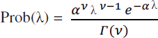
where Γ(ν) is the gamma function, and where parameters α and ν are determined by the mean and variance of λ as:
![]()
That is, the parameters α and ν come from estimates of the mean and variance of λ. For use further below, note that the mean and variance of λ can be expressed in terms of the parameters of the gamma function:
![]()
The gamma distribution is commonly used to approximate the empirical distribution of any continuous, nonnegative random variable because it can represent a variety of distributional shapes, as illustrated in Figure D.1.
PRIOR PROBABILITY DISTRIBUTION OF CATCH PER DAY (X) GIVEN UNCERTAINTY IN MEAN CATCH PER DAY (l)
Given Prob(X) and Prob(λ), the two distributions can be combined to calculate the “prior” probability distribution of total catch per day (X). When Prob(X) and Prob(λ) are combined, it turns out that the resulting prior probability distribution is a negative binomial distribution with parameters α and ν, denoted NegBinprior(X | αprior,νprior), as specified below:
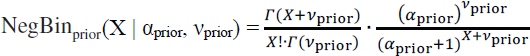
where Γ is the gamma function (as opposed to the gamma distribution), and ! is the factorial operator.
___________________
1 Note that if the data indicate that a normal distribution rather than a gamma distribution fits λ better, there is an alternative version of this model that uses a normal distribution for λ.
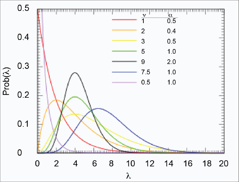
SOURCE: Modified from Wikipedia.org, see https://en.wikipedia.org/wiki/Gamma_distribution.
Interpretation: NegBinprior (X | αprior,νprior) gives the probability distribution of total catch per day for the fishery as a whole (X) for the upcoming fishing season based on the uncertainty (as measured by μprior and ![]() ) in mean total catch per day (λ) as best estimated using MRIP data from the previous fishing season(s).
) in mean total catch per day (λ) as best estimated using MRIP data from the previous fishing season(s).
The negative binomial parameters αprior and νprior are determined by the underlying parameters μprior and ![]() as follows:
as follows:
![]()
For the NegBinprior (X | αprior,νprior) distribution,
![]()
NegBinprior is the “prior” probability distribution of total catch per day (X) for the upcoming fishing season in the sense that it is the best estimate that can be made before (i.e., “prior” to) the beginning of the upcoming fishing season. This prior distribution is based on the best estimates of μprior and ![]() that can be made using MRIP data from past/previous/historical fishing seasons, before the arrival of any new MRIP data from the upcoming fishing season.
that can be made using MRIP data from past/previous/historical fishing seasons, before the arrival of any new MRIP data from the upcoming fishing season.
ESTIMATING THE OPTIMAL FISHING SEASON LENGTH USING THE PRIOR DISTRIBUTION
It is assumed that the fishery manager’s objective is to maximize the fishing season length (measured here in days) while holding the risk (as measured by probability P) of exceeding the ACL below some target level, denoted P*. The prior probability distribution can be used to determine the fishing season length that meets this objective.
At the beginning of the fishing season, before any new information arrives, the prior probability distribution NegBinprior (X | αprior,νprior) gives the best estimate of the probability distribution of fish catch X per fishing day in the season. If “t” days are contemplated for the fishing season, and the probability distribution of fish catch X on each day is negative binomial NegBinprior (X | αprior, νprior), and it is assumed that the daily catches are independent of one another,2 then using statistical formulas for the sums of random variables (see, e.g., Mendenhall et al., 1990, p. 242), one finds that the probability distribution of cumulative fish catch at the end of t fishing days, Xt, (that is, at the end of the contemplated fishing season) is also a negative binomial distribution with parameters α and t•ν, that is, NegBinprior (Xt | αprior,t•νprior). Then:
![]()
and
![]()
To determine the probability P that total fish catch at the end of the season will exceed a given target, say, the ACL, one simply sums the values of NegBinprior (Xt | αprior,t•νprior) from Xt = 0 to Xt = ACL and subtract the sum from 1. That is:
![]()
If fishery managers wish to keep this probability below some target level, say, P*, they should vary the length of the fishing season t until they find the season length t* whereby Prob(Xt > ACL) = P*; a fishing season of length t* is the maximum season length that maintains Prob(Xt > ACL) below P*. Note that this gives an “optimal stopping rule”: stop the season at t* days.
Note also that Excel has a built-in function, NEGBINOM.DIST, that can be used to calculate cumulative negative binomial probabilities (i.e., the negative binomial cumulative distribution function). Using this function:
![]()
and the season length t can be adjusted (using the Solver feature of Excel, for example) until t* is found whereby Prob(Xt > ACL) = P*.
___________________
2 If the daily catches are not independent, that is, if the daily catches are correlated with one another, either positively or negatively, then alternative formulas (Mendenhall et al., 1990, p. 242) that take this correlation into account can be used to calculate the mean and variance of total season catch Xt.
USING BAYESIAN UPDATING TO INCORPORATE NEW INFORMATION, OBTAIN THE POSTERIOR PROBABILITY DISTRIBUTION OF CATCH PER DAY (X), AND UPDATE THE FISHING SEASON LENGTH
As new data arrive during the fishing season, the prior probability distribution of catch per day, NegBinprior(X|αprior,νprior), can be “updated” to take the new data into account. The “updated” probability distribution of catch per day is called the “posterior” distribution because it is “posterior to” (i.e., “after”) the arrival of the new data. Bayes’ rule gives a formula for combining the prior distribution of catch per day, NegBinprior(X|αprior,νprior), with new data to obtain the posterior, updated distribution of catch per day, denoted NegBinpost(X|αpost,νpost).
New data can arrive in different forms. Two likely forms of new data arrival are considered below, but other forms of new data arrival could be analyzed using a similar procedure. For each of the two examples below, the posterior distribution of catch per day derived using Bayes’ rule is given.
Example 1: New Data Arrive in the Form “All Anglers Together Caught n Fish over d Days”
In example 1, after the fishing season begins, managers receive new data that all anglers in the fishery together caught n fish over d days. In this example, there is no uncertainty about the number of fish caught, n. Think of example 1 as a situation of “perfect catch reporting” or “perfect monitoring.” (Example 2 below considers the more likely case of “imperfect catch reporting” with uncertainty in n.)
Using Bayes’ rule, the new data (n, d) can be combined with the prior probability distribution of catch per day, NegBinprior(X|αprior,νprior), to derive the new, updated, posterior probability distribution of catch per day for each day of the fishing season, NegBinpost(X|αpost,νpost), which is also a negative binomial distribution, but with updated parameters αpost and νpost:
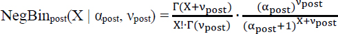
where:
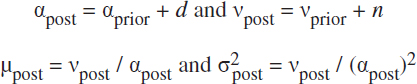
For the NegBinpost(X | αpost,νpost) distribution:
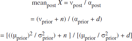
and
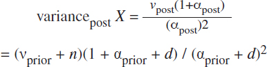
![]()
Note that the updated distribution NegBinpost (X | αpost, νpost) is an update of the distribution of catch per day for all days of the fishing season and as such will be applied to all days of the fishing season, including the days that occurred before the arrival of the new data and the days that occur after the arrival of the new data.
The updated probability distribution of catch per day, NegBinpost(X | αpost,νpost), is then used to update the estimate of the probability distribution of cumulative fish catch at the end of the fishing season, Xt, given by NegBinpost(Xt | αpost, t•νpost), where:
![]()
and
![]()
To determine the updated estimate of the probability P that total fish catch at the end of a fishing season of length t will exceed the given ACL target, the values of NegBinpost(Xt | αpost,t•νpost) from Xt = 0 to Xt = ACL are summed, and that sum is subtracted from 1. That is:
![]()
If fishery managers wish to keep this probability below some target level, say, P*, they should update the length of the fishing season t until they find the updated season length tpost* whereby Prob(Xt > ACL) = P*. A fishing season of length tpost* is the maximum season length that maintains Prob(Xt > ACL) below P*.
Again, Excel has a built-in function, NEGBINOM.DIST, that can be used to calculate cumulative negative binomial probabilities (i.e., the negative binomial cumulative distribution function). Using this function:
![]()
and the season length t can be adjusted (using the Solver feature of Excel, for example) until tpost* is found whereby Prob(Xt > ACL) = P*.
Note that tpost* is the total season length. To find the length of the remaining fishing season, tremaining*, any fishing days that have already occurred in the current season, toccurred, should be subtracted from the total season length. That is tremaining* = tpost* – toccurred.
For each new data update that arrives, the αpost,νpost values from the earlier data update become the new αprior,νprior values that are used with the newly arriving data, and the updating process described above is repeated.
Note that because the arrival of new data will generate new estimates of tremaining*, from the fisher’s point of view, the remaining length of the fishing season is uncertain—fishery managers may need to increase or decrease tremaining* as more data arrive. How confident should fishers be in the estimate of tremaining* at any point in time? At any point in time, the probability that the length of the fishing season will need to be decreased/shortened to avoid exceeding the ACL is given by probability P*, and the probability that the length of the fishing season can be increased/lengthened in the future to “fish as close as we safely can” to the ACL is (1 – P*). So fishery managers can tell fishers: “Based on the data that we have so far this season, our best estimate of the remaining
length of the season is tremaining*, and the probability that the season will need to be shortened is P*, but the probability that the season can be extended is (1 – P*).”
Fishery managers should note that choosing a smaller value for P* reduces the chances of exceeding the ACL but also reduces the length of the remaining fishing season tremaining*. However, choosing a smaller P* also increases the chances (1 – P*) that the remaining fishing season can be increased/lengthened as new data arrive. So choosing a small value for P* is a “good news–bad news, good news” type of decision: good news, the chances of exceeding the ACL are small; bad news, we have to (at this moment) set a short fishing season; good news, there is a high chance (1 – P*) that the fishing season will be extended.
On the other hand, if fishery managers choose a larger value for P*, this will increase the chances of exceeding the ACL but also increase the length of the remaining fishing season tremaining*. However, choosing a larger P* also increases the chances (P*) that the remaining fishing season will need to be decreased/shortened as new data arrive. So choosing a larger value for P* is a “bad news–good news–bad news” type of decision: bad news, the chances of exceeding the ACL are larger; good news, we can (at this moment) set a longer fishing season; bad news, the chances are high (P*) that the fishing season will need to be shortened.
Example 2: New Data Arrive in the Form of New Estimates for the Mean (Μ) and Variance (Σ2) of Catch per Day (l)
In example 2, fishery managers do not benefit from “perfect catch reporting” or “perfect monitoring” during the fishing season, as was assumed in example 1. Instead, after the fishing season begins, managers receive new, but uncertain, estimates of the mean and variance of total catch per day within the fishery. Denote the new estimate of mean catch per day as μnew and the new estimate of the variance of catch per day as σnew2. These new estimates could come from such sources as a new wave of MRIP data or a state data collection program.
Using Bayes’ rule, the new data (μnew,σnew2) can be combined with the prior probability distribution of catch per day, NegBinprior(X | αprior,νprior), to derive the new, updated, posterior probability distribution of catch per day for each day of the fishing season, NegBinpost(X | αpost, νpost), which is also a negative binomial distribution, but with updated parameters αpost and νpost:
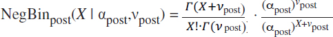
where:
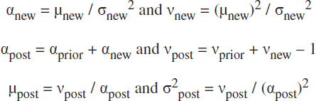
For the NegBinpost(X | αpost,νpost) distribution:
and
Note that the updated distribution NegBinpost(X | αpost,νpost) is an update of the distribution of catch per day for all days of the fishing season and as such will be applied to all days of the fishing season, including the days that occurred before the arrival of the new data and the days that occur after the arrival of the new data:
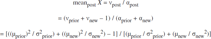
The updated probability distribution of catch per day, NegBinpost(X | αpost,νpost), is then used to update the estimate of the probability distribution of cumulative fish catch at the end of the fishing season, Xt, given by NegBinpost(Xt | αpost,t•νpost), where:
![]()
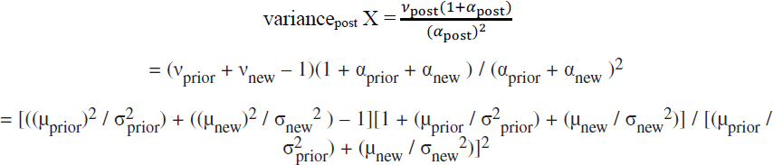
and
![]()
From this point, the procedure used to update the total fishing season length, tpost*, and fishing season length remaining, tremaining*, follows the procedure used in example 1. To determine the updated estimate of the probability P that total fish catch at the end of a fishing season of length t will exceed the given ACL target, the values of NegBinpost(Xt | αpost, t•νpost) from Xt = 0 to Xt = ACL are summed, and that sum is subtracted from 1. That is:
![]()
If fishery managers wish to keep this probability below some target level, say, P*, they should update the length of the fishing season t until they find the updated season length tpost* whereby Prob(Xt > ACL) = P*. A fishing season of length tpost* is the maximum season length that maintains Prob(Xt > ACL) below P*.
Again, Excel has a built-in function, NEGBINOM.DIST, that can be used to calculate cumulative negative binomial probabilities (i.e., the negative binomial cumulative distribution function). Using this function:
![]()
and the season length t can be adjusted (using the Solver feature of Excel, for example) until tpost* is found whereby Prob(Xt > ACL) = P*.
Note that tpost* is the total season length. To find the length of the remaining fishing season, tremaining*, any fishing days that have already occurred in the current season, toccurred, should be subtracted from the total season length. That is, tremaining* = tpost* – toccurred.
As in example 1, for each new data update that arrives, the αpost,νpost values from the earlier data update become the new αprior,νprior values that are used with the newly arriving data, and the updating process described above is repeated.
Similarly, the remarks made in the discussion at the end of example 1 concerning the confidence that fishers should have in tremaining* and the pros and cons of fishery managers setting higher or lower values of P* apply to example 2 as well.
EXTENSIONS AND APPLICATIONS OF THE BASIC BAYESIAN MODEL
Given the basic Bayesian model outlined above, several extensions and applications of the model can be used to address additional questions relevant to in-season management of fisheries under an ACL. For example, the Bayesian model can be used to:
- Compare fishery management outcomes under a fixed season length (“predictability”) with outcomes under a flexible season length (“flexibility”) by running simulations that calculate season length based on prior data only (fixed season length) versus updated season length based on Bayesian updating and new data that arrive throughout the season (flexible season length).
- Demonstrate how Bayesian updating can extend season length by reducing the variance of estimated catch per day, even if the estimated mean catch per day stays constant across the season.
- Assess the value of increasing the frequency of data collection, such as going from a 2-month MRIP wave to a 1-month MRIP wave. Increasing the frequency of MRIP waves allows more rapid Bayesian updating, which can affect, for example, season length and total catch. These outcomes can then be compared against the cost of collecting data more frequently.
- Assess the value of improvements in data quality (improvements in precision, reductions in variance and PSEs). Improvements in data quality would reduce σnew2, which in turn would affect season length and catch. These outcomes can then be compared against the cost of a program to improve data quality.
- Compare the fishery management outcomes (via simulations) of using MRIP estimates of given frequency (e.g., bi-monthly), bias, and precision with estimates from other surveys of potentially different frequency, bias, and precision.
- Combine MRIP estimates with estimates from supplemental surveys whose frequencies, means, and variances may differ from those produced by MRIP, and use the information from both surveys to update the Bayesian model throughout the fishing season. This process would entail two estimates of λ entering the updating process—one from each survey (the estimates of λ could be independent or correlated). Through the Bayesian updating process, survey estimates that are less precise receive less weight in the updating process. This process could be used to simulate adding a state survey, such as Tails ‘n Scales, to MRIP. Or, the process could be used to simulate adding MRIP to a state survey, such as extending MRIP to Texas.
- Accommodate both autocorrelation and contemporaneous correlation in the forecasting process.
- Accommodate correlation in catch across days within a season. For example, if it is known that catch per day increases (or decreases) as a season progresses, this can be taken into account in the Bayesian updating model.
- Accommodate differences in effort between weekend days and weekdays (Powers and Anson, 2016) as catch is accumulated across the days within a season.
- Accommodate changes in fishing season length that result from changes in fishing effort per day (Powers and Anson, 2016, 2019).
- Accommodate separate Bayesian models for recreational-sector catch and commercial-sector catch that can be combined to assess probabilities of meeting sector-specific ACLs and a sector-combined total-catch ACL.
- Accommodate separate Bayesian models for different geographic regions that can be combined to assess probabilities of meeting region-specific ACLs and a combined-region total-catch ACL.
- Make the best use of any available information in data-poor fisheries. Any available data from prior years could be used to form priors, or a noninformative prior could be used. Simulations could be used to assess the implications of alternative priors and the length of time it would take for any differences in outcomes, based on differences in the priors, to become negligible. As another alternative, expert opinion on maximum and minimum catch-per-day values could be used with a uniform distribution (a noninformative prior, conditional on the maximum and minimum values) to obtain a mean and variance for a prior.
- Assess the differences in proposed catch carry-over (overage and underage) policies across years via simulation. For example, when an underage increases the ACL in the subsequent year or an overage decreases the ACL in the subsequent year, the model can be used to estimate the effects on the probability distribution of season length in the subsequent year.
- Assess via simulation whether particular ancillary variables (e.g., weather, water temperature, fuel prices, unemployment rate) (Powers and Anson, 2016) could potentially reduce reducing uncertainty σnew in2priors . by reducing σprior2 or reduce uncertainty in new or updated data by
- Assess via simulation how new technologies (e.g., dockside cameras) that increase data collection frequency (thereby increasing the frequency of Bayesian updating within a season) or improve data quality (and thereby reduce σnew2) would affect expected fishery management outcomes. The simulations could also be used to investigate the effects of the use of more frequent but lower-quality data on expected fishery management outcomes.
REFERENCES
Clark, C. 1990. Mathematical Bioeconomics: The Optimal Management of Renewable Resources, 2nd Edition. New York: Wiley.
Mendenhall, W., D. Wackerly, and R. Scheaffer. 1990. Mathematical Statistics with Applications, 4th Edition. Boston, MA: PWS-Kent.
Powers, S. P., and K. Anson. 2016. Estimating recreational effort in the Gulf of Mexico Red Snapper fishery using boat ramp cameras: Reduction in federal season length does not proportionally reduce catch. North American Journal of Fisheries Management 36(5):1156–1166. https://doi.org/10.1080/02755947.2016.1198284.
Powers, S. P., and K. Anson. 2019. Compression and relaxation of fishing effort in response to changes in length of fishing season for Red Snapper (Lutjanus campechanus) in the northern Gulf of Mexico. Fisheries Bulletin 117:1–7. https://doi.org/10.7755/FB.117.1.1.
Ross, S., M. 2010. Introduction to Probability Models, 10th Edition. Oxford, UK: Academic Press.


