
Appendix B
Leveraging Covariances and Conditionals
THE COVARIANCE OF CATCH ESTIMATES ACROSS MRIP DOMAINS
The Marine Recreational Information Program (MRIP) provides estimates of fish catch and its variance by domain, where a domain is defined as a combination of fish species, 2-month wave time period, geographic state or substate location, fishing area (inshore, state ocean waters, or federal ocean waters), and fishing mode (private boat, shore-based, charter, or headboat). Typically, fishery managers use information from only one domain to forecast catch for that domain. Doing so neglects information in patterns that may exist in the data across domains that could be useful for increasing the precision (decreasing the percent standard errors [PSEs]) of catch and effort forecasts, such as those made for the purpose of in-season management by fishery managers using the MRIP output estimates.
MRIP produces a catch estimate for a given domain by multiplying an estimate of fishing “effort” (i.e., fishing trips) for the domain obtained from the Fishing Effort Survey (FES) by an estimate of the “catch per unit effort,” or CPUE (i.e., catch per fishing trip), obtained from the Access Point Angler Intercept Survey (APAIS) for the domain. The MRIP estimates are weighted such that the effort estimate from FES is statistically independent of the CPUE estimate from APAIS within a domain. However, the effort estimate in one domain may not be statistically independent of the effort estimate in another domain. Similarly, the CPUE estimate in one domain may not be statistically independent of the CPUE estimate in another domain.
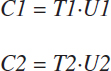
As an example, consider MRIP catch estimates for two domains, where estimated catch in the first domain is C1, and estimated catch in the second domain is C2. For example, C1 might be the catch of a particular species in a particular location in a particular wave, and C2 might be the catch of a different species in that same location and wave. The MRIP estimates these catches by multiplying together weighted estimates of effort (trips) in each domain, E1 and E2, with weighted CPUE in each domain, U1 and U2:
When the fish catch in one domain moves in the same direction as the fish catch in the other domain, the covariance between the two fish catches is positive. When the catches move in opposite directions, the covariance between the catches in the two domains is negative. The general definition of the covariance between the catches across the two domains, cov(C1,C2), is:
![]()
By the definition of covariance:
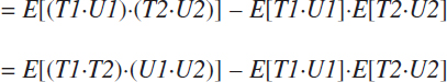
By the independence of T and U within a domain:
![]()
By the definition of cov[(T1∙T2),(U1∙U2)]:
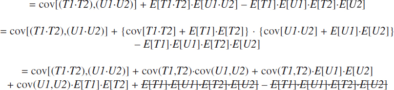
or, finally:
![]()
Therefore, the covariance between catches across domains, or cov(C1,C2), may be nonzero when any of the following is nonzero:
- covariance in the product of effort (T1∙T2) and the product of CPUE (U1∙U2) across domains (i.e., cov[(T1∙T2),(U1∙U2)]);
- covariance in effort across domains, cov(T1,T2); or
- covariance in CPUE across domains, cov(U1,U2).
The examples below illustrate how nonzero covariances could occur in many situations.
The covariance in the product of effort (T1∙T2) and the product of CPUE (U1∙U2) across domains (i.e., cov[(T1∙T2),(U1∙U2)]) could be nonzero in some situations. For example, Gillig et al. (2000) investigated the effect of Red Snapper CPUE (from the Marine Recreational Fisheries Statistics Society on fishing effort (trips per angler) targeting Red Snapper for reef fish anglers in the Gulf of Mexico in 1991. In this cross-sectional study, these investigators found that CPUE was correlated with fishing effort. Specifically, the authors found that “a 10 percent increase in catch rate [CPUE] will result in a 14.6 percent increase in the number of recreational Red Snapper trips [T].” This implies that the covariance between fishing effort and CPUE across locations is not zero; for example, if CPUE is high in two locations in a particular time period, then, all else being equal, one would expect fishing effort to be high in those two locations in the same time period. Similarly, the covariance between fishing effort and CPUE across time periods may be nonzero; for example, if CPUE is relatively high in a particular location for two time periods, then, all else being equal, one might expect that fishing effort would be relatively high in that location for those two time periods.
In the example where C1 is the catch of a particular species targeted in a particular location in a particular time period, and C2 is the catch of a different species targeted in that same location and time period, then cov(T1,T2) is clearly positive, as both species experience the same number of trips in a particular location and time period (see Table B.1). If the FES-estimated number of trips for species 1 in a particular location and time, namely T1, were larger (say, in a different, hypothetical, FES sample drawn at that same location and time—an FES resampling experiment), then the FES-estimated number of trips for species 2 in the same location and time, namely T2, would also be larger, and by the same amount, because the FES estimate of the number of trips for that location and time would be applied to both species.
Similarly, suppose the two species are found in the same locations and are typically caught together (on a given trip). In this case, if the APAIS estimate of the catch rate for the first species, U1, increases (say, because a different, hypothetical, APAIS sample was drawn from the anglers present at that location and time—an APAIS resampling experiment), then the APAIS estimate of the catch rate for the second species, U2, would also increase, because U1 and U2 would be calculated from the same sample of APAIS anglers, and species 1 and species 2 would have been caught together. In this case, cov(U1,U2) would be positive (see Table B.2). On the other hand, if species 1 and species 2 are typically not caught together (on a given trip), then APAIS samples (hypothetically, drawn from the same population of anglers at a given location and time) resulting in a higher estimate of U1 might result in a lower estimate of U2, and cov(U1,U2) would be negative (see Table B.3).
Comparing catches of a single species at two different locations over time (either across years
TABLE B.1 Positive cov(T1,T2) for Two Targeted Species at the Same Location and Time
| Species 1 Effort (T1) |
Species 2 Effort (T2) |
|
|---|---|---|
| Sample 1 | 8 | 8 |
| Sample 2 | 10 | 10 |
| Sample 3 | 6 | 6 |
| Sample 4 | 7 | 7 |
| cov(T1,T2) | 2.9167 | |
TABLE B.2 Positive cov(U1,U2) for Two Species Typically Caught Together
| Species 1 CPUE (U1) |
Species 2 CPUE (U2) |
|
|---|---|---|
| Sample 1 | 3 | 5 |
| Sample 2 | 5 | 7 |
| Sample 3 | 10 | 15 |
| Sample 4 | 2 | 3 |
| cov(U1,U2) | 18.6667 | |
TABLE B.3 Negative cov(U1,U2) for Two Species Typically Not Caught Together
| Species 1 CPUE (U1) |
Species 2 CPUE (U2) |
|
|---|---|---|
| Sample 1 | 3 | 10 |
| Sample 2 | 8 | 2 |
| Sample 3 | 10 | 2 |
| Sample 4 | 1 | 6 |
| cov(U1,U2) | –12.6667 | |
or across waves within a year), where C1 is the catch of the species in one location, and C2 is the catch of the same species in a different location, cov(C1,C2) would be positive if the abundance of the species were similar at both locations at the same time (see Table B.4). On the other hand, cov(C1,C2) would be negative if high abundance at one location were typically paired with low abundance at the other location at a given time (see Table B.5). The value of cov(C1,C2), where C1 and C2 represent catches in different locations, could be due to covariance in trips across locations, cov(T1,T2); covariance in CPUE across locations, cov(U1,U2); or both.
Comparing catches of a single species at two different times (either two different years or two different waves) for a set of locations, where C1 is the catch of the species at time 1, and C2 is the catch of the same species at a later time 2, cov(C1,C2) would be positive if the size of the catch were similar at both times for a given location (see Table B.6). On the other hand, if a large catch in one time period were associated with a small catch in the other time period at the same location, then cov(C1,C2) would be negative (see Table B.7). The value of cov(C1,C2) where C1 and C2 represent catches in different time periods could be due to covariance in trips across time periods, cov(T1,T2); covariance in CPUE across time periods, cov(U1,U2); or both.
USING CONDITIONING TO REDUCE CATCH VARIANCE AND PSEs
In some situations, the probability distribution of one variable, say, fish catch in a particular MRIP domain, C, may depend in part on the value of another variable, say, X. In such cases, one would say that the probability distribution of C is conditional on the value of X, expressed as P(C|X), and that X is a conditioning variable for C. For example, suppose the catch of Wahoo off the coast of North Carolina in June, C, depends in part on the water temperature off the coast of
TABLE B.4 Positive cov(C1,C2) for a Single Species Across Location 1 and Location 2
| Catch C1 Location 1 |
Catch C2 Location 2 |
|
|---|---|---|
| Time 1 | 3 | 3 |
| Time 2 | 5 | 5 |
| Time 3 | 10 | 10 |
| Time 4 | 2 | 2 |
| cov(C1,C2) | 12.66667 | |
TABLE B.5 Negative cov(C1,C2) for a Single Species Across Location 1 and Location 2
| Catch C1 Location 1 |
Catch C2 Location 2 |
|
|---|---|---|
| Time 1 | 3 | 5 |
| Time 2 | 5 | 3 |
| Time 3 | 10 | 2 |
| Time 4 | 2 | 10 |
| cov(C1,C2) | –10 | |
TABLE B.6 Positive cov(C1,C2) for a Single Species Across Time 1 and Time 2
| Catch C1 Time 1 |
Catch C2 Time 2 |
|
|---|---|---|
| Location 1 | 3 | 3 |
| Location 2 | 5 | 5 |
| Location 3 | 10 | 10 |
| Location 4 | 2 | 2 |
| cov(C1,C2) | 12.66667 | |
TABLE B.7 Negative cov(C1,C2) for a Single Species Across Time 1 and Time 2
| Catch C1 Time 1 |
Catch C2 Time 2 |
|
|---|---|---|
| Location 1 | 3 | 5 |
| Location 2 | 5 | 3 |
| Location 3 | 10 | 2 |
| Location 4 | 2 | 10 |
| cov(C1,C2) | –10 | |
North Carolina in May, X. In this case, P(C|X) says that the probability of catching various numbers of Wahoo off the coast of North Carolina in June depends on the water temperature off the coast of North Carolina in May.
The conditioning variable X could be anything that affects the probability distribution of C. For example, X could be the catch of the same fish species in some other place or season, or the catch of some other species in a particular place or season, or a weather variable (air temperature or precipitation), or an ocean conditions variable (wave height, seawater temperature, current, tide, El Niño, etc.), or an economic conditions variable (unemployment rate, fuel price, etc.), or a cultural variable (holidays, hunting season, etc.), or a fishery regulation variable (length of fish season, bag limit, size limit, etc.).
There can be more than one conditioning variable (more than one X) for C. For example, the probability of catching various numbers of Wahoo off the coast of North Carolina in June might depend on the weather (which affects angler effort), the estimate of the Wahoo stock size (from a stock assessment), and an estimate of the abundance of Wahoo prey (which attract Wahoo to this particular area), as well as water temperature. In this case, C might be conditional on all of these variables. In practice, fishery managers would want to focus on the conditioning variables that have the largest effect on C, and those variables for which data are readily available or cheap to collect.
For the purposes of this discussion, the focus is on a single conditioning variable, X, say, water temperature.
In practice, the probability distribution of C conditional on X, that is, P(C|X), is calculated by looking back in time at the MRIP catch estimates of C and comparing them with the various values of X. For example, if water temperature were 75°F, then the probabilities of catching various numbers of Wahoo would be P(C|X = 75), but if water temperature were 80°F, then the probabilities of catching various numbers of Wahoo would be P(C|X = 80), and so on.
The expected value of C conditional on X, that is, the average value of C for a particular value of X, is denoted E[C|X]. If fishery managers looked back at the MRIP estimates of C when X = 75, and then took the average of the MRIP estimates of C when X = 75, the result would be E[C|X = 75]. The same could be done for other values of X (E[C|X = 65], E[X|X = 85], etc.).
Note that the expected value of the conditional expectation of C, given X, that is, E[E[C|X]], is an unbiased estimate of E[C] (Ross, 1988, p. 286):
![]()
For example, the formula above says that if one takes E[C|X = 75], E[C|X = 80], E[C|X = 85], etc., for all of the different values of water temperature X and then averages them all together, then one derives the average value of C across all the different possible values of water temperature X.
The conditional variance of C with respect to X, Var(C|X), is defined as (Ross, 1988, p. 292):
![]()
The above formula gives the variance of catch for a particular value of X, say, the variance in Wahoo catch for a particular water temperature.
By taking the expectation of Var(C|X) and combining the result with the definition of Var(E[C|X]), the conditional variance formula (Ross 1988, p. 292) below can be derived:
![]()
Rearranging:
![]()
By the definition of variance, Var(C) > 0, Var(C|X) ≥ 0, and hence E[Var(C|X)] ≥ 0.
Thus:
![]()
The last formula above is a very important result. It says, for example, that the variance in Wahoo catch at a particular water temperature is less than the variance of Wahoo catch across all water temperatures. The formula implies that if one knows (or can estimate/forecast) a good conditioning variable X (such as water temperature in the present example), then one can reduce the variance in one’s forecast of C (Wahoo catch) below the variance estimate provided by MRIP by taking the conditioning variable, such as water temperature, into account. If fishery managers could find a good conditioning variable X, they could use it to reduce the variance (and PSE) of the catch forecast, which would allow more precise in-season management—fishery managers could “manage closer to the ACL.”
In summary, the method of conditioning might be useful to fishery managers because E[E[C|X]] is an unbiased estimate of E[C], and Var(E[C|X]) is smaller than Var(C).
COVARIANCES, CONDITIONAL EXPECTATIONS, AND FORECASTS
Suppose that fishery managers wish to forecast the catch, C, of a species in a particular location and wave/season (i.e., in a particular MRIP domain), and information is available on a good conditioning variable, X (see the section above). The conditioning variable X could be the catch of the same species in a different location or wave/season, or the catch of a different species in the same (or different) location or wave/season, or X could be some ancillary variable, such as water temperature, wind speed, or fuel price. Suppose managers wish to use the value of X to help forecast the value of C.
Let f(X) be a “prediction function” that attempts to predict C based on X. The “best” prediction function, defined as the (unbiased) prediction function that minimizes the variance of the prediction, is the expected value of C conditional on X, that is, E(C|X).
Note that the best predictor E[C|X] is an unbiased estimator of E[C]:
![]()
Note further that the variance of the best predictor E[C|X] is less than the variance of any other predictor f(X) based on X; that is:
![]()
If the joint probability distribution of C and X were not completely known, or the analytical calculation of E[C|X] were mathematically difficult, then E[C|X] could be simulated, or the discussion could be limited to a common class of prediction functions, such as linear prediction functions, f(x) = a + bX. The best linear prediction function E[C|X] (i.e., the function that results in an unbiased prediction with minimum variance within the class of linear prediction functions) is (proof: Ross, 1988, p. 298):
![]()
where E[E[C|X]] = E[C], that is, the predictor is unbiased, and where the mean squared error (MSE) of the conditional prediction is (proof: Ross, 1988, p. 298):
![]()
For the special (but common) case in which C and X jointly have a bivariate normal distribution, the expectation of C conditional on X, that is, E(C|X), is, in fact, linear in X, and so the above results give the best possible predictor for C and its MSE among all possible predictors (not just within the class of linear predictors) (proof: Ross, 1988, p. 299).
Note the importance of the covariance between C and the conditioning variable X, that is, cov(C,X), in the formula for MSE. The larger the covariance, cov(C,X), the smaller is the MSE of the conditional prediction. In fact, the MSE decreases with the square of the covariance between C and X. Also, the smaller the value of var(X), the smaller is the MSE. Hence, when attempting to identify good candidates for a conditioning variable X, fishery managers should search for X variables that have a large value of cov(C,X) and a small value of var(X).
With respect to software implementation, MRIP uses SAS Proc Survey means to conduct its data analyses, and Proc Survey means can calculate conditional means and variances. If fishery managers identified the variable X and provided MRIP with data on X, then MRIP could add the data on variable X to the MRIP dataset, and E(C|X), cov(C,X), and MSE(E[C|X]) could easily be calculated by SAS Proc Survey means and released by MRIP for subsequent use by fishery managers.
THE ROLE OF COVARIANCE WHEN FISHERY MANAGERS AGGREGATE OR DISAGGREGATE MRIP CATCH ESTIMATES
The covariance between fish catch X in one MRIP domain and fish catch Y in a different MRIP domain can affect the variance (and PSE) of a catch forecast in situations in which fishery managers aggregate or disaggregate the domain-level fish catch estimates X and Y provided by MRIP. The discussion below does not refer to the methodology used by MRIP to calculate the catch estimates X and Y and the variances (and PSEs) of X and Y; instead, it refers to fishery managers’ subsequent use of MRIP estimates to produce catch forecasts using the catch estimates and PSEs that have been produced and disseminated by MRIP.
Aggregating Fish Catches Across Domains
Covariance can be important when one is aggregating fish catches across domains, such as aggregating the catch of a particular species across geographic regions, across time periods (i.e., across waves or across years), or across fishing modes; aggregating the catch of related species into a species-group total (such as aggregating the catches of various Grouper species into total catch of all Groupers); or aggregating the catch across all species to obtain the “total catch of all fish” at a given location and time period.
In general, the variance of the aggregated fish catch X + Y depends on the variance of X, the variance of Y, and the covariance of X and Y, as given by (Ross, 1988, p. 276):
![]()
If the fish catches X and Y are independent, then cov(X,Y) is zero, and the variance of the aggregated fish catch is correctly calculated by simply summing the variances of X and Y provided by MRIP:
![]()
However, suppose fishery managers assume that the fish catches X and Y are independent and that cov(X,Y) is zero when in fact the catches are dependent and cov(X,Y) ≠ 0. If catches X and Y are dependent and cov(X,Y) is not zero, then omitting the covariance may lead to over- or underestimation of the variance (and PSEs) of the aggregated catch.
If cov(X,Y) is in fact negative and if it is omitted from the calculation of var(X + Y), then var(X + Y) and PSEs of the forecast will be overestimated. PSEs will appear larger than they actually are, resulting in fishery regulations that are more stringent than they need to be to avoid catches that exceed an annual catch limit (ACL). Thus, correctly including cov(X,Y) in the calculation of var(X + Y) will reduce var(X + Y) and PSEs, allowing for less stringent fishery regulations.
Perhaps equally important, if cov(X,Y) is in fact positive and if it is omitted from the calculation of var(X + Y), then var(X + Y) and PSEs of the forecast will be underestimated. In this case, fishery regulations based on the PSEs may be too lax, resulting in catches that exceed ACLs more often than expected by fishery managers. In this case, correctly including cov(X,Y) in the calculation of var(X + Y) will increase var(X + Y) and PSEs, resulting in stricter fishery regulations that keep catches below the ACL as often as fishery managers expect.
Disaggregating Fish Catches Across Domains
Recognizing the importance of covariances is also important when one is disaggregating fish catches across domains (e.g., when disaggregating total regional fish catch into catches by subregion, when disaggregating total fish catch into catches by fishing mode, or when disaggregating total catch of a species group into catches by species [such as disaggregating total Grouper catch into catches by species of Grouper]).
In general, the variance of the disaggregated fish catch X depends on the variance of the aggregated fish catch X + Y, the variance of Y, and the covariance of X and Y:
![]()
If the fish catches X and Y are independent, then cov(X,Y) is zero, and the variance of the disaggregated fish catch var(X) is correctly calculated by simply subtracting MRIP-supplied var(Y) from the MRIP-supplied variance of the aggregated catch var(X + Y):
![]()
However, suppose fishery managers assume that the fish catches X and Y are independent and that cov(X,Y) is zero when in fact the catches are dependent and cov(X,Y) ≠ 0. If catches X and Y are dependent and cov(X,Y) is not zero, then omitting the covariance may lead to over- or underestimation of the variance (and PSEs) of the disaggregated catch.
If cov(X,Y) is in fact negative and if it is omitted from the calculation of var(X), then var(X) and PSEs will be underestimated. In this case, fishery regulations based on the mistakenly small PSEs may be too lax, resulting in catches that exceed ACLs more often than managers expect. In this case, correctly including cov(X,Y) in the calculation of var(X) will increase var(X) and PSEs, resulting in stricter fishery regulations that keep catches below the ACL as often as managers expect.
On the other hand, if cov(X,Y) is in fact positive and if it is omitted from the calculation of var(X), then var(X) and PSEs will be overestimated. PSEs will appear larger than they actually are, resulting in fishery regulations that are more stringent than they need to be to avoid catches that exceed an ACL. Thus, correctly including cov(X,Y) in the calculation of var(X) will reduce var(X) and PSEs, allowing fishery regulations to be relaxed.
Extension to More Than Two Domains
The issues discussed in this section extend to aggregation or disaggregation of catches across more than two domains (e.g., more than two time periods, more than two species). When more than two domains are involved, the covariances between all pairs of domains can affect the variance of the result.
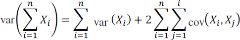
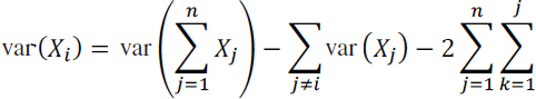
The general variance formula for aggregating across n domains, X1, X2, …, Xn, is given by (Ross, 1988, p. 276):
The formula for the variance of Xi disaggregated from Xj≠i is given by:
LIKELIHOOD OF NEGATIVE COVARIANCES AMONG SPECIES IN A MULTISPECIES FISHERY CONSTRAINED BY A BINDING ACL
In a multispecies fishery constrained by a binding ACL, such as perhaps the South Atlantic Snapper-Grouper fishery, one might expect covariances across catches to be negative among species in the fishery. One possible reason for this is illustrated by the following example.
Suppose there are r species in the multispecies fishery, indexed i = 1 to r. Suppose the proportion of each species i in the multispecies population is Pi, such that ∑i P = 1, and suppose that fish are caught in proportion to their prevalence in the multispecies population; that is, the probability that a fish caught by an angler is of species i is given by Pi. Suppose that each cast by an angler is independent of every other cast by that angler and is also independent of the casts made by other anglers (the example could be modified to include correlation among casts, but that is not the primary point here). Suppose Ni is the catch of species i by all anglers in the fishery in a specified time period. Let C be the total catch of all species in a multispecies fishery constrained by an ACL, such that C = ∑iNi = 1 = ACL. In this situation, the joint probability of all the anglers together catching the combination of fish (N1,N2, …, Nr) is given by the multinomial distribution (Ross, 1988, p. 282):

and the covariance between the catch of species i, Ni, and species j, Nj, is:
![]()
The above covariance is negative, and it is larger in magnitude for larger values of the ACL and for species pairs that are larger proportions Pi and Pj of the total multispecies population.
USE OF CONTROL VARIATES TO REDUCE THE VARIANCE OF CATCH FORECASTS
Covariances across MRIP domains might also be used to reduce catch variances through the use of control variates. For example, suppose that fish catch in domain i is Xi, and fishery managers are interested in reducing the variance (and PSE) of Xi. Suppose further that catch Xi can be aggregated with fish catch in domain j, Xj, to produce aggregated catch (Xi + Xj), where the aggregated catch has mean E(Xi + Xj) = μ.
Construct the artificial “control variate” variable, W:
![]()
Note that the mean value of W, E[W], is the same as the mean value of Xi, E[Xi]. The variance of W is given by:
![]()
The value of “a” that minimizes var(W) can be determined by taking the partial derivative of var(W) with respect to a, setting the partial derivative equal to zero, and solving for a to find:
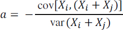
Substituting the value of “a” into var(W) and simplifying:
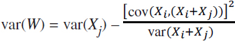
Since it is always the case that var(Xi + Xj) > 0 and[cov(Xi, (Xi + Xj))]2 ≥ 0, it is always the case that:
![]()
and as long as cov[Xi,(Xi + Xj)] is not zero, whether positive or negative, it is the case that:
![]()
Thus, the fishery in domain i could be managed by tracking the control variate W rather than catch Xi, where W has the same mean (expected value) as Xi, but the variance (and PSE) of W is smaller than the variance (PSE) of Xi.
Note that the degree of variance reduction increases with the square of cov[Xi,(Xi + Xj)], the covariance between Xi and (Xi + Xj).
Note also that the control variate technique might be useful across various types of domains. For example, Xi and Xj could be the catches of two species in a multispecies fishery, or Xi and Xj could be the recreational and commercial catch of the same species, or Xi and Xj could be the catches of the same species in two different geographic regions, or Xi and Xj could be the catches of the same species at two different time periods. The control variate technique might be especially useful for the catch of a rare-event species Xi that is correlated with the total catch (Xi + Xj) of a fishery of which the rare-event species is a part (e.g., a particular rare-event species of Grouper that is part of the total catch of all Grouper species in a particular location).
REFERENCES
Gillig, D., T. Ozuna, Jr., and W. L. Griffin. 2000. The value of the Gulf of Mexico recreational Red Snapper fishery. Marine Resource Economics 15:127–139.
Ross, S. 1988. A First Course in Probability, 3rd Edition. New York: Macmillan.


