9
Biofuels

This chapter focuses on biofuels for transportation, how they are produced, and how to use lifecycle analysis (LCA) to assess their climate impacts. First, this chapter briefly summarizes several different broad categories of biofuels, either currently in production or near commercialization, and then evaluates the types of feedstocks used to produce biofuels. Next the special considerations in the assessment of attributional, supply-chain emissions from biofuel production are discussed. Last, several LCA methodologies used to assess the market-mediated effects attributable to biofuels are summarized.

The primary motivating factors to produce biofuels have been to reduce reliance on petroleum products, to enhance energy security, and to create new markets for agricultural products. Scarcity and price volatility of petroleum fuels provided important early motivation for interest in biofuels, going back for a century and peaking during periods of high oil prices or concerns about continued availability. More recently, concern over climate change caused primarily by the combustion of fossil fuels added a new motivation to seek alternative fuels produced from biogenic feedstocks that can in principle reduce greenhouse gas (GHG) emissions while also reducing exposure of U.S. consumers to oil price volatility. Market development, including price support, for agricultural products has also been a key motivation for biofuel production, and agricultural producers have been actively involved in the development and promotion of biofuels (Chambers et al., 1979; Gasparatos et al., 2013; Hill, 2022; Keeney 2009; Khanna et al., 2008; Lark et al., 2022; Robertson et al., 2008; Tilman et al. 2009; Tyner and Taheripour, 2007, 2014).

There have also been long-standing concerns about biofuels, including their contribution to climate change and their merits compared to mitigation efforts. This historically took the form of debates over net energy balance of different biofuels, and more recently have focused on life-cycle GHG emissions, air quality, and water quality. Other concerns include increased costs to taxpayers and consumers, competition for land, increased food prices, net energy balance, GHG impacts, and negative impacts on air and water quality impacts, biodiversity, and other environmental concerns (Chambers et al., 1979; Gasparatos et al., 2013; Hill, 2022; Keeney 2009; Khanna et al., 2008; Lark et al., 2022; Robertson et al., 2008; Tilman et al. 2009).

• “Food versus fuel” concerns that expanded production of biofuels compete with food consumption, driving up food prices and harming food consumers, especially poor food consumers.
• Land use change (LUC) due to biofuels, including claims that expanded use of biofuels leads to expansion of agricultural acreage at the expense of forest or grassland ecosystems in the U.S. Midwest or in the tropics.
• Potential for other environmental damages

For context in considering these potential benefits and concerns, the policy environment both at home and abroad is discussed in this chapter.

BIOFUEL FEEDSTOCKS AND FINISHED FUELS

Categories of Finished Biofuels

At their most basic level, biofuels are composed of molecules that include carbon that was recently removed from the atmosphere by photosynthesis, in contrast to carbon originating from fossil resources. Though the feedstocks for these fuels are biogenic in origin, their production may use fossil inputs in some parts of their supply chain, which must be accounted for in LCAs. Depending on the specific fuel, biofuels may be produced from sugars, starches, lipids, cellulose, lignin, and other compounds derived from mixed organic waste, or from woody or herbaceous biomass. Liquid biofuels target four markets: gasoline (for spark-ignited internal combustion engines), diesel (for compression-ignited internal combustion engines), jet fuel (for jet engines), and marine fuel (for compression-ignited internal combustion engines on marine vessels). Gaseous biofuels require additional changes to vehicles and engines to accommodate their onboard storage and use; these fuels also require separate fueling infrastructure. Compressed biomethane, derived from biogas produced during anaerobic digestion and sometimes referred to as renewable natural gas, can also be used in vehicles that are equipped to run on compressed natural gas. Additionally, hydrogen can be produced from biomass through gasification or reforming of biomethane for use in fuel cell vehicles.

Ethanol

The most common biofuel in use currently in the United States is ethanol, which is produced through microbial fermentation of sugars and is suitable as a blendstock for spark-ignited internal combustion engines. Ethanol production facilities primarily use yeast to convert sugars to ethanol, namely Saccharomyces cerevisiae (also known as brewer’s yeast). S. cerevisiae and other, less common hosts naturally produce ethanol under anaerobic conditions, meaning in the absence of oxygen. If the starting feedstock is a polysaccharide such as starch, as is the case for the corn ethanol industry, a mixture of enzymes is first required to break it down into glucose (C₆H₁₂O₆). Sucrose (C₁₂H₂₂O₁₁), which is the sugar present in sugarcane juice, can be utilized directly by yeast to produce ethanol. One of the challenges facing cellulosic biofuel producers is associated with the limited ability of some microbial hosts to efficiently utilize sugars derived from biomass. In these cases, a cocktail of enzymes is also required to depolymerize the polysaccharides present in cellulose and hemicellulose portions of cell walls, such as glucan and xylan, to their corresponding monosaccharides. The second-most abundant sugar liberated from plant cell walls is xylose (C₅H₁₀O₅), and common hosts for ethanol production do not naturally utilize five-carbon sugars. Co-utilizing strains (meaning they utilize both five- and six-carbon sugars) have been developed and are being continually improved. More advanced hosts are also being developed to utilize other plant-derived monomers, including aromatic compounds liberated from lignin (Linger et al., 2014).

Ethanol in the United States is produced almost exclusively from corn starch, with 15.8 billion gallons of production, 14.6 billion gallons blended with gasoline, and net exports of 1.2 billion gallons in 2019 (U.S. Energy Information Administration, 2019). The volumetric blending rate was about 10.25 percent in that year. At a 10 percent volumetric blend rate, ethanol can be used in most existing fueling stations

and combusted in most spark-ignited internal combustion engines without any adjustments. Because ethanol’s lower heating value is 21.1 MJ/liter, as compared to a typical gasoline lower heating value of 32.0 MJ/liter, vehicles deemed “flex-fuel” require modifications to the fuel pump and fuel injection system, as well as the engine control module, to account for this difference in heating value and ethanol’s oxygen content. These flex-fuel vehicles are capable of using blends of up to 83 percent ethanol in gasoline.¹ Flex-fuel vehicles can run on a blend known as E85 which, contrary to what its name might suggest, is gasoline blended with anywhere between 51 percent and 83 percent ethanol by volume.

Biodiesel

Biodiesel (fatty acid methyl esters) is the second most common liquid biofuel produced in the United States. Biodiesel is suitable as a neat fuel (100 percent) or for blending with diesel for use in compression-ignited internal combustion engines. It is produced by reacting fats or oils with short-chain alcohols such as ethanol or methanol in the presence of a catalyst; this process is called transesterification. The result is a 10:1 ratio of biodiesel and glycerin (a co-product). Total production in 2020 was 1.8 billion gallons, with 45 percent of that volume being used as a neat fuel and 55 percent used in blends with petroleum-derived diesel fuel. Soybean oil is the largest feedstock for producing biodiesel in the United States, followed by smaller, roughly equal amounts of corn oil, canola oil, and yellow grease (a waste product). Algae are also capable of producing oils suitable for conversion to biofuels, although the cost of production and the effort required to lyse the cell walls to extract the oils have hindered commercialization of the technology (Cruce and Quinn, 2019). Other organisms can produce oils; for example, oleaginous yeast strains can convert sugars to oils, but those cells must also be lysed to recover the product (Sitepu et al., 2014).

Aviation Biofuels

A wide array of biomass feedstocks including grains, sugar crops, oilseeds, lignocellulosic crops, and waste materials can be processed into alternative aviation biofuels via chemical, biological, and hybrid biological-chemical routes. These pathways require additional processing, certification and testing to ensure that they meet the physiochemical characteristics of conventional jet fuel at certain technology-specific blending rates. To date, there are no commercially-approved aviation biofuel pathways suitable for use at a 100 percent blend rate, with the maximum allowed share limited to 50 percent. See Chapter 8 for more information on approved pathways and relevant life-cycle methodologies.

Biomethane

Biomethane refers to biogenic methane produced from a variety of feedstocks and conversion processes, including decomposition in landfills, anaerobic digestion of biogenic wastes and residues, and gasification of biomass in conjunction with a methanation reaction. Depending on the process used to produce the biomethane, its purity (i.e., its methane content) can vary significantly; at lower methane concentrations (approximately 50 percent), it is typically referred to as biogas. This biogas can be combusted onsite for electricity or heat, or alternatively, upgraded to remove impurities such as sulfur and carbon monoxide to make it suitable for distribution on the natural gas grid for use in natural gas vehicles or at natural gas power plants.

Drop-In Fuels

The term “drop-in fuel” is something of a misnomer because most alternative fuels cannot serve as neat replacements for petroleum fuels. However, drop-in fuels do tend to have heating values closer to those

___________________

¹ See: https://afdc.energy.gov/vehicles/how-do-flexible-fuel-cars-work.

of conventional petroleum fuels and may be suitable at higher blending levels than, for example, ethanol (Taptich et al., 2018). Renewable diesel is an example of a drop-in fuel. Unlike biodiesel, renewable diesel can encompass a variety of production processes, including biological or thermochemical, that result in hydrocarbons suitable for use in compression-ignited internal combustion engines.² One of the simpler methods for producing renewable diesel is to hydrotreat oils and fats to remove the oxygen molecules (deoxygenate). Hydroprocessed esters and fatty acids (HEFA) fuel is produced by a similar process but is intended for use as a jet fuel blendstock. Hydroprocessed esters and fatty acids synthetic paraffinic kerosene (HEFA-SPK) is produced by hydrodeoxygenation followed by cracking and isomerization of the paraffinic molecules to produce molecules of the desired chain length for jet fuels.

A commonality among renewable diesel and HEFA production processes is the need for hydrogen, which is used to deoxygenate the feedstock and isomerize the finished fuel. Therefore, the source of hydrogen can influence the emissions attributable to these biofuels, ranging from more emissions-intensive fossil hydrogen to alternative sources such as green hydrogen produced using electrolysis of renewable energy (more discussion of hydrogen LCA considerations is available in Chapter 7).

FEEDSTOCKS FOR BIOFUEL PRODUCTION

Agricultural Feedstocks

Corn and soybeans are the most common feedstocks currently used to produce biofuels in the United States. Corn grain is the primary source of domestic ethanol production and, as mentioned earlier, soybean oil is the primary feedstock for domestic biodiesel production. Agricultural residues, such as corn stover and wheat straw, are also potential biofuel feedstocks. Sugarcane, while not a major crop inside the United States, is an important bioenergy crop globally (mostly in Brazil), and the residues (bagasse and trash) can serve as lignocellulosic feedstocks in addition to the sucrose that is currently fermented to produce fuel. Other types of dedicated so-called energy crops that can be used as biofuel feedstocks include energy grasses like switchgrass and Miscanthus, diverse native prairie biomass, and short rotation woody crops, although these are not yet produced at commercial scale for biofuels (Field et al., 2020; Tilman et al., 2006). Cover crops, which are crops grown primarily for the purpose of maintaining or enhancing the productivity of the land between main crop harvests, also can be used as feedstock for biofuel production.

A key distinction among different agricultural feedstocks is between perennial and annual crops. Unlike annual crops which must be replanted each harvest, perennial bioenergy crops may live for a decade or longer. Rather than requiring steady inputs each year, perennial crops have increased inputs during establishment year(s) and reduced inputs once they are fully established. High-yielding perennial grasses like switchgrass and Miscanthus, and diverse mixtures of native prairie species, are sometimes credited for their potential to restore soil carbon because of the reduced disturbances to soils associated with perennial agronomic practices and because of the substantial accumulation of below-ground carbon in the roots and rhizomes, although this net sequestration does not continue indefinitely. This reduced soil disturbance associated with perennial crops is also why they are sometimes cited as being appropriate to grow on marginal lands that are not suitable for food production (Keeler et al., 2013), although the definition of what constitutes marginal land is hotly debated (Khanna et al., 2021).

Woody Biomass

Woody biomass is one of the most abundant feedstock for bioenergy production in the United States. Wood is used to produce pellets, briquettes, and logs, which are often categorized as densified biomass fuel. The total capacity of densified biomass fuel manufactured in the United States is about 13 million tons/year, and most of them are for wood pellet production. In the United States, wood pellets are made from forest residues from managed forest or wood residues from industrial plants such as sawmills and

___________________

² See https://afdc.energy.gov/fuels/emerging_hydrocarbon.html.

wood product manufacturing facilities. Densified wood pellets in the United States are made from diverse feedstocks, including residues from industrial plants (e.g., sawmills and wood product manufacturing facilities and roundwood (also referred as stemwood) harvested from managed forest (about 20 percent of total feedstock in 2018) (Lan et al., 2021; Liu et al., 2017a). As a waste material from forest management and wood processing activities, forest residues can be a source of biorefineries for biofuel production. LCAs have been conducted for biofuels made from forest residues (e.g., Hsu, 2012; Lan et al., 2019; Nie and Bi, 2018). For roundwood, most of the LCA studies have focused on the solid fuel products instead of liquid biofuels (Liu et al., 2017b; Verkerk et al., 2018).

Biomass Wastes and Residues

In addition to purpose-grown crops, biofuels can be produced from wastes and residues of other primary products. This category is extremely varied, with a great variety of physical and economic differences between different wastes and residues, and very different life-cycle implications depending on the material in question. Though many feedstocks in this category are lignocellulosic, they may also include gaseous feedstocks and lipids. For example, straw and residues typically left on the field or used as animal fodder can be converted into biofuel; alternately, biogenic wastes or by-products from industrial processes, such as inedible beef tallow or used cooking oil from restaurants can also be converted into biofuel. The life-cycle approach to study the impacts of these feedstocks will necessarily vary based on the product in question, as discussed in Chapter 6.

Algae

Biofuel can be produced from algae, which is grown in open ponds or in closed photobioreactors (Tu et al., 2017). These systems can be located on land that is not used for agriculture; moreover the productivity per unit land area of algal systems can be high compared to land plants.

KEY CONSIDERATIONS IN BIOFUEL LIFE-CYCLE ANALYSIS

This section assesses several key aspects of life-cycle methods particular to biofuels. First, the existing methods used to assess the attributional supply chain emissions attributable to purpose-grown biomass feedstocks and the emissions attributable to biorefineries are discussed. Next, is a discussion of several market-mediated effects attributable to biofuel policies, and a discussion of existing approaches and methods to assess the emissions impacts of these effects. Last, the degree to which different market-mediated effects have been assessed and factored into existing biofuel policies is discussed.

Attributional Effects of Biofuels

Agricultural Feedstock Production

LCA methods commonly used to estimate GHG emissions associated with crop production in conventional agricultural systems are largely similar regardless of the specific crop in question. Emission sources include the production and use of agricultural equipment (e.g., tractors) and fertilizers, herbicides, and pesticides. For perennial crops, an average may be taken, or other allocations may be made, across the lifetime of the crop to account for year-to-year variations in yields and inputs. An array of land management practices can affect emissions associated with feedstock production. These practices include tillage, the use of nitrification inhibitors, animal manure application, crop rotation, and cover cropping (Lee et al., 2020). Each of these management practices must be evaluated on a life-cycle basis because there can be tradeoffs between on-farm emissions and upstream or market-mediated effects. For example, while nitrification

inhibitors reduce nitrous oxide (N₂O) emissions on-field, GHGs are emitted during their production. Furthermore, the effects of land management practices can vary depending on location given differences in soil quality, crop yield, and climate conditions (Hill et al., 2019; Maestrini and Basso, 2018; Qin et al., 2018). Many of these factors, along with soil properties, also affect N₂O emissions from soils, which can vary widely (Lawrence et al., 2021; Sathaye et al., 2011; Shakoor et al., 2021).

There are strong spatial variations in emissions from land management practices for agriculture (Adler et al., 2012). Chapter 4 discusses the influence of methodological aspects of spatial effects in more detail, including for soil carbon changes that are one of the most important outcomes of land management effects.

Because LCA results are spatially dependent, increasing transparency and availability of public data pertaining to agricultural inputs at finer spatial scales may improve LCA parameterization. Currently, the U.S. Department of Agriculture publishes critical statistics of farm energy use and fertilizer consumption every five years with yield estimates published annually. More frequent data collection may also highlight how key parameters such as these change during years with extreme weather events and would facilitate statistical and machine learning based approaches to estimating fertilizer and energy consumption under different farming conditions (e.g., economic, climate, policy). The finest spatial scale generally available is county-level given concerns around protecting farmers’ proprietary information. See Chapter 5 for a discussion of verification strategies that can be used to develop farm-level feedstock information in the absence of publicly available databases.

There have been numerous examples of estimates of supply chain GHG emissions for conventional agriculturally-derived feedstocks using a variety of LCA methods (Hill et al., 2019; Smith et al., 2017). It is important to remember that LCA results for feedstocks can vary spatially and temporally because of a variety of factors including technological advances, uptake of land management practices, soil characteristics, market conditions, policy changes, and climate change among other factors. Understanding these spatial and temporal variations and how they change over time may be used to improve aspects of estimates of biofuel life-cycle GHG emissions and how they evolve with changing climate, market, and policy conditions.

Woody Biomass Production

The GHG emissions associated with the production of woody biomass come from multiple sources, including the use of energy and materials (e.g., fertilizers and soil amendments) for forest management, harvesting, storage and transportation. Energy-related GHG emissions can be estimated by fuel consumption and the GHG emission factors of each fuel. The fuel consumption depends on wood species and forest operations. For example, thinning is a common practice that generates forest residues and is used in the United States to address issues such as bark beetles and wildfires (Knapp et al., 2021). Diesel fuels are often used for activities involved in commercial thinning, such as felling and bunching, skidding, delimbing, debarking, and loading (Markewitz, 2006; McEwan, Brink, and Spinelli, 2019; Oneil et al., 2010). Similar activities are involved in logging (in other words, final harvesting), but the diesel inputs are often different. The GHG emissions of machinery used for thinning and logging can be estimated by using the diesel consumption data and emission factors of diesel (Lan et al., 2019).

Herbicide, fertilizers, and soil amendments used in the forest site preparation and planting generate GHG emissions from the applications and upstream production. The data of upstream GHG emissions are available in many life-cycle inventory (LCI) databases. These upstream GHG emissions have large variations, depending on the chemicals and materials used and production technologies. GHG emissions may also be generated during and after the application of fertilizers, and may depend on fertilizer type. For example, compared to many other nitrogen-containing fertilizers, urea may have lower carbon dioxide (CO₂) emissions during the production stage but higher CO₂ emissions after field application due to the CO₂ generated after urea hydrolysis (Hasler et al., 2015). The GHG emissions released by fertilizers can be estimated by emission factors and application rates (Brentrup et al., 2000). Therefore, the GHG emissions related to the materials and chemicals used in forest management need to be transparently reported with additional information in production technology, supply chain (e.g., transportation modes), and application methods and rates (e.g., in the unit kg/ha).

The storage of most woody biomass generates GHG emissions from energy use and fugitive emissions. The energy use of woody biomass storage is generally low (Sahoo et al., 2018). Fugitive emissions are contributed by chemical and biological degradation, including CO₂, methane (CH₄), and other volatile hydrocarbons (Alakoski et al., 2016; Geronimo et al., 2022), and may vary substantially. The large variations of fugitive emissions depend on many factors such as the shape and sizes of both biomass and piles, moisture control strategies, storage methods, the type of biomass, and the local environment. The research on these fugitive emissions is more-limited compared to GHG emissions studied in other stages related to woody biomass production.

The GHG emissions of woody biomass transportation are driven by the weight of biomass, distances, and energy use. The weight of biomass and distances depend on the biomass supply chain design. Centralized design requires the transportation of woody biomass directly to a biorefinery while decentralized design often pretreats woody biomass by drying and/or size reduction for easier and more economic transportation (Lan et al., 2021). Main GHG emissions sources are energy that is used for activities such as loading, hauling, and transporting (mostly by truck). Transportation GHG emissions can be estimated using either energy-based approach discussed previously, or weight–distance based emission factors (e.g., data in the USLCI database reported on the basis of 1 t*km).

The source of wood used affects the GHG emissions of biomass production in several aspects. In many cases the feedstocks of biofuels are residues generated from forestry operations or wood manufacturing (e.g., sawdust and barks). As residues are also produced from forestry operations, allocating GHG emissions of forestry operations and other activities between the main products (e.g., logs) and other products is often needed, and the allocation methods affect the LCA results (see discussion below on allocation). It may be challenging to use system expansion to avoid allocation in this case due to the lack of alternative product routes for logs and residues. However, system expansion could be helpful to include counterfactual scenarios of alternative uses and/or fates of residues. For example, Lan et al. (2020) explored the counterfactual scenarios of forest residues. Residues from forest operations are currently either left on site to decay are combusted without energy recovery (Booth, 2018). Mill residues are sent to landfills, burned for energy recovery, or sold to market to produce other wood products like particleboard (Lan et al., 2020). These counterfactual scenarios could be considered for estimating avoided emissions (see section on Negative Emissions), although they are commonly not included in biofuel LCAs using forest residues (Lan et al., 2021) except for several studies focusing on developing global warming potential (GWP) indicators for biogenic CO₂ emissions that consider slow residue decomposition if not collected (Liu et al., 2017a, 2017b). The source of wood also affects the carbon flows associated with effects related to forest management practices. The source of wood determines the forest management and relevant direct GHG emissions given the differences in forestry operations for diverse wood species and regional climate.

The source of wood may have different carbon implications due to changes in land use and forest management practices. For example, the wood from afforestation and reforestation brings carbon benefits of increased carbon stocks on lands (Favero et al., 2020; Kauppi et al., 2020). The carbon implications of using woody biomass for biofuels are complicated, and depends on how the forest and related systems will be affected (Klein et al., 2015); see discussion of biogenic emissions accounting in Chapter 6. The use of

forest residues may provide financial incentives for using overstocked, low-quality biomass that reduce forest wildfires and associated GHG emissions (Verkerk et al., 2018). Excessive removal of forest residues affects the forest soil and growth (Achat et al., 2015). The rapid increase of roundwood harvest rate may lead to decrease of carbon stock (Pingoud et al., 2020); however, the increased demand of woody biomass could also stimulate new forests and better forest management for additional carbon storage benefits (Cowie et al., 2020; Favero et al., 2020). The forest carbon stock changes are closely linked to the biogenic carbon issues of forests (see section on biogenic carbon in Chapter 6). Previous studies also show the reduced climate benefits if the policy supporting the use of forest reduces timber supply for material applications (Favero et al., 2020). Thereforeit is important that a practitioner consider the impacts of using woody biomass on forest management in LCAs. It may be challenging to directly assess the future forest carbon stock changes caused by different forest management strategies and under diverse climate change situations. However, it is useful to at least explore the potential impacts of key parameters or assumptions of forest management practices that could be changed in response to increased demand of woody biomass, such as changes in tree species, thinning, residue removal, and forest productivity (Klein et al., 2015).

In sum, estimates of the GHG emissions from woody biomass production depend on the source of wood, forest management (i.e., the application of fertilizers, pesticides, and soil amendments), logistics design, and the accounting methods of biogenic carbon. The use of residues and primary product logs from the forest sector may lead to different impacts and resulting carbon implications depending on the category of woody biomass used and where it is produced, such as carbon emissions or reductions from LUC, changing forest management practices in response to increased woody biomass demand, and counterfactual scenarios of alternative uses and fates of residues. However, data gaps exist in fugitive GHG emissions of woody biomass storage.

CARBON EMISSIONS AND SEQUESTRATION FROM BIOREFINERIES

GHG emissions associated with biomass conversion come from multiple sources, including on-site combustion of fuels (e.g., fossil fuels, biomass, or byproducts), direct emissions from conversion processes, and upstream emissions associated with the production of chemicals, enzymes, and electricity used by biorefineries. There may be a key distinction between biogenic (sometimes referred to as “contemporary”) carbon and fossil carbon for purposes of carbon accounting—the atmosphere is not affected differently by them. Some studies include biogenic carbon emitted in the form of CO₂, then balanced with a biogenic CO₂ sequestration credit during the biomass growth phase (e.g., Spatari et al., 2005), while other studies exclude them by using the carbon neutral assumption (e.g., Cai et al., 2013; Scown et al., 2012). It is important to note that the form of carbon can change in conversion (e.g., carbon as CO₂ fixed by photosynthesis but released as CH₄, with a different GWP. It is critical to clearly identify the individual contributors to GHG emissions and sequestration for biomass conversion. If a CO₂ sequestration credit is applied to account for biomass regrowth, this should be differentiated from any soil organic carbon sequestration credits (or net emissions) included in the analysis. GHG emissions from biorefineries can be measured when emission monitoring systems are available, and organic carbon testing has been considered in regulations related to

biomass content. They can also be estimated using the mass and energy balance data collected from biorefineries (primary data), literature (secondary data), or derived from mechanistic process simulations (Huo et al., 2009). The energy balances provide energy demand information that can be used together with GHG emissions factors of fuels to compute the energy-related emissions (Lan et al., 2020). The energy-related emissions can also be estimated by mechanistic modeling for the combustion processes in biorefineries (Cai et al., 2018). Depending on the source and quantity of fuel used, the energy-related GHG emissions vary; for example, using renewable electricity or increasing the efficiency of a biorefinery could reduce its energy-related emissions. The mass balance data can provide estimations of process-related GHG emissions as they are parts of gas outputs of biorefineries.

Process-related GHG emissions can be estimated by theoretical estimations or mechanistic process models, and these emissions are often process- and technology-specific. For example, ethanol biorefineries generate significant biogenic CO₂ emissions in the fermentation process, which was estimated to be 45 Mt/year for 216 existing biorefineries in the United States (Sanchez et al., 2018) using an emission factor of 2853 metric ton of CO₂/million gallons of ethanol produced. Such an emission factor was estimated based on the stoichiometry of converting glucose to ethanol and CO₂ (Hornafius and Hornafius, 2015). Another example is biomass gasification that can produce various biofuel products using different downstream processes, such as ethanol, methanol, hydrogen, Fischer–Tropsch fuels and many others. CO₂ is part of the gas products from gasification and the quantity of CO₂ depends on many factors such as feedstock compositions, gasifiers, operational conditions, and downstream cleaning up processes (Sikarwar et al., 2017). Given the complexity of chemical reactions and downstream processes involved in gasification, theoretical estimations of CO₂ emissions based on chemical reactions could be challenging. Mechanistic models such as process simulations using software AspenPlus have been used to simulate the CO₂ gas stream for gasification to different types of biofuels (Susmozas et al., 2016; Salkuyeh et al., 2018).

CO₂ emissions of biomass conversion could be mitigated by integrating carbon capture into biorefineries, though the impact on biorefinery emissions depends on the CO₂ capture rate, the end use of the captured CO₂, and the fate of stored CO₂. Ethanol plants have been considered near-term candidates for carbon capture (Sanchez et al., 2018), while other biomass conversion pathways such as gasification also attract increasing interest given the significant amount of CO₂ generated as by-products (Sikarwar et al., 2017). The quantity of CO₂ that can be removed by carbon capture depends on many factors such as technology choices, CO₂ concentrations, and end-of-life of CO₂ (e.g., geological storage or utilized for other applications such as enhanced oil recovery that may lead to secondary leakage, as well as increased oil use). As CO₂ capture facilities need additional energy input, they may change the energy generation and supply scheme of biorefineries. The energy demand of CO₂ capture facilities in biorefineries could be met by burning byproducts (e.g., solid residues), expanding the capacity of on-site energy generation facilities, or purchasing fuels externally (Kim et al., 2020). That being said, this requirement is less for the CO₂ by-product of fermentation, which does not require gas-phase separation, only dewatering and compression. Different choices will affect the GHG emissions associated with the energy consumption of CO₂ capture facilities, but mass and energy balance approaches have been used to estimate energy use and energy-related GHG emissions (Yang et al., 2020).

There are GHG emissions generated during the upstream production of chemicals, enzymes, and electricity purchased by biorefineries. These emission data can be obtained from LCI databases and literature (e.g., the life-cycle GHG emissions of electricity generation are available in databases such as the USLCI database [National Renewable Energy Laboratory, 2012] and literature [Sathaye et al., 2011]). As these GHG emissions highly depend on the technology pathways and market mix, the GHG emission factors with technology and market mix information are should be disclosed for biofuel LCA.

In addition to biofuels, biorefineries almost always produce byproducts or co-products. The distinction between what materials qualify as co-products and what outputs are truly waste products is often unclear. For corn ethanol facilities, distiller’s dried grains with solubles and corn oil are common co-products that have clear applications in the animal feed market and can be accounted for through allocation procedures (see Chapter 3). From the standpoint of carbon flows, it is a safe assumption that all of the carbon in these products will eventually be oxidized, some as methane from ruminants. Co-products or

byproducts from other biorefining processes, particularly if the product(s) do not have a well-established market, can be more difficult to account for.

Biochar, a byproduct from most thermochemical conversion processes, is an example of a product for which a robust market does not yet exist (Baker et al., 2020; Campbell et al., 2018). In general, biochar is made of aromatic compounds and is rich in carbon (> 65 percent by mass), although the composition varies widely depending on the biomass feedstock and process conditions under which it was produced (Ippolito et al., 2020). Char can be combusted as a fuel on-site or exported to be used as a fuel elsewhere, in which case the carbon accounting can be calculated using system expansion, assuming the fuel it is displacing (e.g., coal or natural gas) is known. If biochar is applied to soils with the intention of improving soil quality or sequestering carbon, the impact is highly uncertain and is the topic of heated debate (Dumortier et al., 2020; Lan et al., 2021; Maroušek et al., 2017). In the Getting to Neutral report by Lawrence Livermore National Lab (Baker et al., 2020), researchers assumed that 80 percent of carbon in biochar buried underground would remain sequestered for at least 100 years but they chose not to attempt to capture the impacts on net primary productivity (if applied to croplands or other lands). This is similar to the assumption used in Woolf et al. (2012) and Breunig et al. (2019), both of which assume that 85 percent of carbon in biochar is recalcitrant over a 100-year period. The assumptions used in these studies are consistent with biochar research that shows high carbon persistence in biochar, although the biochar decomposition rate depends on many factors, such as pyrolysis temperature and biomass composition (Joseph et al., 2021; Lehmann, 2021; Woolf et al., 2021). One advantage for biochar, in terms of its recalcitrance, is that it contains little in the way of nutrients, meaning that microbial breakdown of biochar in the environment, if buried in large quantities, should be slow (Astals et al., 2012; Moset et al., 2015; Pognani et al., 2009).

Another common byproduct of bioenergy production is solid digestate; this is particularly prevalent for anaerobic digestion facilities, where a typical facility only breaks down 20-40 percent of solids in the digester and the remaining material must be directly land-applied, composted, or sent to landfills (Astals et al., 2012; Moset et al., 2015; Pognani et al., 2009). This material will vary in its composition depending on the original feedstock type, residence time in the digester, and digester conditions, but the average carbon content for digestate produced from manure or mixed organic waste is estimated to be 18-25 percent on a dry mass basis (European Commission, 2018). In contrast to biochar, digestate is rich in nutrients, which means it has value as a fertilizer supplement and any carbon sequestration potential is negligible as remaining carbon-containing compounds will be broken down rapidly by microbes once the digestate is directly land-applied or composted. In addition, its use is a potential source of N₂O emissions.

The role of CH₄ emissions in low-carbon fuel production systems is important in the context of anaerobic digestion facilities (e.g., wastewater treatment facilities and manure digesters). Regardless of whether the carbon is biogenic or fossil, methane emissions must be accounted for. For consistency, peer-reviewed LCA literature and regulatory applications tend to use GWP₁₀₀ (i.e., global warming potential calculated over 100 years) values for all non-CO₂ GHGs. In systems that produce CH₄, fugitive emissions are often most easily and transparently calculated as a fraction of total system throughput, as is common practice in government-sponsored GHG inventories, such as the Environmental Protection Agency (EPA) GHG Inventory³ and the California Air Resources Board’s GHG inventory.⁴ This can be applied to different parts of the supply chain, including production, processing/cleanup, and pipeline transport. However, measurement and monitoring is required to ensure these estimates are accurate; Alvarez et al. suggested that prior fugitive CH₄ emissions estimates were likely too low, and the leakage from the oil and gas supply chain was the equivalent of 2.3 percent of all natural gas produced, as of 2015 (Alvarez et al., 2018). Though the authors did not estimate the equivalent effect across biomethane supply chains, fugitive CH₄ leaks may pose similar risks (see Chapter 7). Regular monitoring of fugitive CH₄ emissions from anaerobic digestion and any other methane-producing facilities will be necessary to ensure that accurate leakage values are incorporated into CI values.

___________________

³ See: https://www.epa.gov/ghgemissions/inventory-us-greenhouse-gas-emissions-and-sinks.

⁴ See: https://ww2.arb.ca.gov/ghg-inventory-data.

Using allocation or system expansion to include the substitution benefits of byproducts is common in biofuel LCA. If the substitution benefits of byproducts are included, the use of byproducts and counterpart products to be replaced has direct impacts on the GHG emissions allocated to biofuel. Therefore, the information of byproduct applications, substitution effects, and the GHG emissions of counterpart products and materials is to be disclosed and documented.

To summarize, mass or energy balance are the most common methods used to estimate GHG emissions of biorefineries. Some of the attributional GHG emissions of upstream production of electricity and chemicals used in biomass conversion are available in many LCI databases but have large variations depending on the production technologies and market mix. Research articles vary in their assumptions about the potential for carbon sequestration using biorefinery co-products as soil amendments; but many assume 80–85 percent of biochar is stable for at least 100 years whereas digestate and compost are not assumed to result in accumulation of stable carbon in soils.

Market-Mediated Effects of Biofuels

Large-scale production of biofuels has an effect on various markets at regional, national, or global scales and can affect market prices at these levels. Changes in market prices can trigger other changes in production and consumption decisions that may have positive or negative effects on GHG emissions from those markets. These secondary effects on GHG emissions are of concern because they affect the assumed savings in GHG emissions obtained by displacing fossil fuels by biofuels. In this section, several relevant effects attributable to increased biofuel demand are identified, then several methods used to assess their impacts are discussed.

Competition for Land

Biofuels produced from agricultural feedstocks, including food and feed crops, perennial energy crops, or short rotation woody crops, compete for land with crops produced for non-biofuel uses. The extent to which this is the case will depend on the type of feedstock, the yield of feedstock per unit of land, and the types and availability of land on which they can be grown. The use of food or feed crops for biofuels could divert some of the produced crops from food or feed consumption. If land resources are not fully employed (idle land is available) and the supply function for a given crop is relatively elastic, then additional biofuel production would increase production of the food crop with a more limited increase in the price of the food crop. However, the diversion of the food crop to biofuel could increase the price of the food/feed crop. Increases in biofuel production could also lead to changes on the extensive margin by bringing additional land into crop production, by conversion of idle land, pastureland, and forestland to cropland.

It may also lead to reduction in the amount of the food crop exported (if the country is an exporter) for agricultural commodities or an increase in imports of agricultural commodities. If the country is a major exporter (importer) of food/feed crops with a large share of world market trade, the increased demand for biofuel crops could reduce exports (increase imports) of food/feed crops, and this can potentially affect world market prices of those crops, leading to increased returns to producing those crops in other countries and to intensive and extensive margin changes in land use in those countries.

The use of non-food feedstocks, such as dedicated energy crops, could also divert land from food crops; the extent to which this is the case may be less than for food crops, because these crops can potentially be grown on low quality/marginal land not suitable for other crops, and they may be high yielding and thus require less land to produce a given amount of biofuel. However, to the extent that their production increases demand for land and diverts some land from food crops and raises land rents, they could also create similar incentives for LUCs at the intensive and extensive margin as in the case of food crops. Higher prices of food crops and agricultural commodities will lead to similar changes in trade in agricultural commodities as described above.

The extent of LUC and the type of land (idle land, pastureland, forestland) conversion induced by biofuels will depend on various features of the feedstock, such as its yield, requirements for soil fertility and quality, climatic conditions, its co-products, the potential to make changes in crop production at the intensive margin (e.g., yield improvement and expansion in harvest frequency due to cultivation of unused cropland), and availability and ease of conversion of various types of non-cropland to crop production. The extent of LUC associated with a given volume of biofuels is expected to change over time in response to changes in crop varieties, crop productivity, management practices, changes in the climate conditions and so on. As the production of biofuel feedstocks increases, there may be an increase in demand for land and an increase in the returns to land and in food or feed crop prices within the country. This effect could be non-linear if additional land brought into production has a yield lower than the existing cropland. Additionally, increases in crop prices can induce changes in management practices that can increase land productivity. Furthermore, the availability of idle land is also expected to change over time, depending on the rate of growth of demand for food or feed relative to the rate of growth of crop productivity, urban development, government policy support for agriculture, and other factors. Induced LUC is therefore a dynamic phenomenon that cannot be proxied by a fixed estimate that is constant over time.

The resulting changes in land use both at the intensive and extensive margins within the country and globally can affect GHG emissions. Intensive use of existing cropland, due to additional chemical applications, can increase GHG emissions not only on land under biofuel feedstocks but on other cropland as well. While fertilizers used for biofuel crop production enter directly into the LCA of biofuels, an increase in the rate of fertilizer application on other cropland could generate some additional GHG emissions as a market-mediated effect in response to biofuel demand. Similarly, if due to extensification carbon-rich grasslands and forestland are converted to crop production, this could release stored carbon into the atmosphere (Fargione et al., 2008; Gibbs et al., 2008; Hertel et al., 2010).

There are several key factors that can influence estimates for ILUC values for a given biofuel pathway, including: changes in the mix of crops induced by biofuel production, modeling yield change per harvest, modeling change in harvest frequency (including multiple cropping and returning unused land to crop production), the share of additional land expansion that goes on high carbon stock land, elasticities, emission factors and amortization time horizon.

Displacement of Fossil Fuels

In principle, large scale biofuel production could displace at least a portion of domestic liquid fossil fuels consumption, ostensibly reducing oil demand. If the production of biofuels does reduce the world market price of oil, then it has the potential to increase the demand for oil in the rest of the world. This has

been referred to as the “global rebound effect” which might offset the savings due to biofuel (Hill et al., 2016).

The effect of a reduction in the world oil price on the domestic oil price in the biofuel-producing country is complex and depends on the domestic biofuel and agricultural policies used to promote the production of biofuels in a given country (Taheripour and Tyner, 2014). In general, biofuel blend mandates, such as the U.S. Renewable Fuel Standard (RFS), and low-carbon fuel standards (LCFSs), are designed to implicitly penalize the consumption of fossil fuels and implicitly subsidize the consumption of biofuels with a lower carbon intensity (CI) than an LCFS. The implicit subsidy will depend on the policy, for example, in the case of an LCFS, the implicit subsidy increases as the CI of the biofuel decreases relative to an LCFS; in contrast with a biofuel blend mandate, the subsidy may be the same for all biofuels covered by the mandate.

Other Indirect Effects

While the above two effects have received the greatest attention in the literature, biofuel production affects production and consumption decisions in other markets that can also affect GHG emissions. Specifically, the production of corn ethanol results in the production of co-product distillers dried grain solubles which are used as animal feed and can replace corn and soymeal to some extent. Higher crop prices due to corn ethanol are expected to reduce demand for livestock and this could reduce downstream emissions generated during the production of livestock, which are largely in the form of CH₄ and thus have a higher GWP than carbon emissions. Additionally, feeding distiller’s dried grain solubles to cattle affects their digestion and reduces or increases (Masse et al., 2014) enteric CH₄ emissions generated by them (Arora et al., 2010; Bremer et al., 2010; Flugge et al., 2017). Similarly, policies that lead to increased corn ethanol production may also support animal feed production by generating additional distillers dried grain solubles, which incentivizes animal production over plant-based protein sources for human consumption.

Another unintended consequence of demand for biomass for advanced biofuels is the increase in the demand for advanced biofuel feedstocks, such as corn stover. This can create incentives to change crop rotations from corn-soybean rotation to continuous corn rotation. Since corn is more nitrogen fertilizer intensive this can lead to an increase in fertilizer use as corn displaces soybean production. Also, corn stover harvesting practices can be accompanied by increased fertilizer inputs, particularly at higher residue removal rates. It can also lead to a change in tillage methods and use of better varieties of seeds that produce larger agricultural biomass (stover) which can increase carbon sequestration in biomass and soils and reduce atmospheric carbon, although this can depress grain yield leading to the unintended consequence of induced LUC.

Another unintended consequence is dietary change, which may include both food availability and dietary consumption in response to biofuel demand. For example, models used to assess LUC have estimated that increased biofuel production has reduced calories from corn and wheat used for food and feed by 25–50 percent (Searchinger et al., 2015). Also, for example, using more biofuels byproducts such as distillers dried grain solubles and oilseed meals has helped the livestock industry to move towards producing more meat from non-ruminants with lower CI than ruminant meat (Taheripour et al., 2021). The consequences of these changes are complex and can both increase and decrease net GHG emissions.

In addition to induced LUCs and the rebound effect, the existing literature has noted several other indirect effects due to biofuels—such as co-product impacts on livestock markets, food availability and dietary change—that may affect GHG implications positively or negatively.

QUANTIFYING MARKET-MEDIATED EMISSIONS FROM BIOFUELS

Land Use Change

Assessment of the GHG intensity due to market-mediated effects of biofuels uses a comparison of production and consumption in multiple markets in the economy both domestically and in the rest of the world with biofuels and in a counterfactual scenario without biofuels (holding all else constant). This assessment is commonly conducted using various types of economic models; these models can be classified broadly into partial equilibrium (PE) and computable general equilibrium (CGE) models. Some of these models are global and can analyze both domestic and international LUCs, whereas others only analyze domestic LUCs in the country that produces biofuels.

Partial Equilibrium (PE) models consider only a few sectors of the economy that are most closely affected by biofuel production, such as the agricultural, forestry and fuel sectors. Prices, production, and land allocation within these sectors are determined within the model, and it is assumed that conditions in the rest of the economy remain unchanged with biofuel production. These models could be either static or dynamic and used to analyze the effects of a one-time shock in biofuel demand on equilibrium prices and quantities in the markets included in the model. A widely used example of this is the Food and Agricultural Policy Research Institute (FAPRI) model, developed at Iowa State University’s Center for Agricultural and Rural Development (CARD) (e.g., Searchinger et al., 2008; Fabiosa et al., 2010). These models include multiple markets, each of which is represented by a demand and supply relationship that are linked across markets through cross-price elasticities. As a result, changes in demand in one market can affect prices and production in other connected markets. These models estimate the demand for land converted based on assumptions about crop productivity and allocates the expansion in demand for cropland in each region among other types of land cover including forest and grassland categories based on a land allocation process.

These models are suited to analyze the effects of changes in demand for existing crops that are already being produced but not readily adaptable to analyze the effects of introducing new biofuel feedstocks, such as dedicated energy crops that are yet to be commercially produced. Early applications of the FAPRI-CARD model to examine the induced LUC effect of biofuels ignored the potential for conversion of cropland pasture or idle land to crop production before converting forestland. The inclusion of cropland pasture or idle land in later versions of this model was found to substantially reduce the modeled conversion of forestland to crop production by the model (Dumortier et al., 2011).

Other well-known PE models used in assessing induced LUCs due to biofuels are the Forest and Agricultural Sector Optimization Model (FASOM) and the Global Biomass Optimization Model (GLOBIOM). Unlike static multimarket models that are reduced form models of supply and demand, these are dynamic programming models. They are multi-period, structural models that represent the behavior of utility maximizing consumers and profit maximizing producers. They typically include detailed biophysical data to model the dynamics of crop yields, soil carbon changes, and GHG emissions. These models can be regional or global in scope: with examples including FASOM and the Biofuel and Environmental Policy Analysis Model (BEPAM), which are national scale models for the United States and GLOBIOM, which is at the global scale. These models examine the effects of biofuel production on land allocation, equilibrium production, and prices subject to constraints on land, technology, and various material balances, and solve for endogenous prices, production and consumption decisions in multiple markets within a limited number of sectors of the economy. In these models, land is allocated among alternatives based on returns to land and LUCs can occur at the intensive and extensive margin based on relative returns to alternative uses. These “bottom-up” models can incorporate detailed representation of the technology, introduce new technologies and crops and substantial spatial heterogeneity in land availability, land suitability, and costs of production across fine spatial scales (Khanna and Crago, 2012; Khanna et al., 2014). The national scale models are not suited to calculate the global induced LUC but can calculate domestic induced LUC. They can also be linked to other global models to calculate the international portion of the induced LUC as in

Beach and McCarl (2010). EPA (2010) has used FASOM in combination with FAPRI-CARD to assess induced LUC values for corn ethanol, soy biodiesel, sugarcane ethanol, and switchgrass ethanol.

CGE models simulate economy-wide effects of a biofuels shock, include intersectoral linkages and constraints on labor and capital and determine all prices and incomes in the economy simultaneously. These models are typically global in scope, represent multiple economic sectors in each region, and include factor markets for labor and capital. While these models are broad in geographic and sectoral scope, many CGE models have limited spatial resolution and usually partition the world into several large homogenous geographical units called agro-ecological zones. In these models each region or country has a representative household that allocates resources across uses domestically and consumes goods and services produced domestically or imported. Some CGE models may have more than one representative household. On the production side, multiple producers demand primary and intermediate inputs (produced domestically or imported) and produce goods and services. Primary inputs are typically land, labor, capital, and resources. In these models the government collects taxes and pays subsidies or makes transfer payments. Each region interacts with other regions through trade. These models assume that consumers maximize utility and producers maximize profits in a perfectly competitive market setting, leading to endogenously determined prices and quantities of goods and services and also factors of production. These models typically limit the number of agricultural products considered by categorizing individual commodities into large groups (e.g., all coarse grains, oilseeds) and imposing the same behavioral and market assumptions on the individual components. Among the CGE models being used are the Global Trade Analysis Project (GTAP-BIO), the Modeling International Relationships in Applied General Equilibrium (MIRAGE) and the Emissions Prediction and Policy Analysis (EPPA) models (Gurgel et al., 2007; Hertel et al., 2010; Laborde and Valin 2012; Taheripour et al., 2017). In determining induced LUCs due to biofuels, these models do not divide induced LUCs into direct and indirect. However, CGE models usually provide induced LUCs by geographical regions. These models distinguish between different types of land and the ease of conversion of land from one type to another is determined by an elasticity of transformation in GTAP-BIO and by a cost of conversion in EPPA. For more details on modeling LUCs in CGE models see Taheripour et al. (2020).

In addition to structural differences across the PE and CGE models, they also differ in key assumptions that affect LUC in response to biofuel production. Some of the key assumptions are described in the rest of this section.

Land Productivity in Intensive and Extensive Margins. The effect of a biofuel policy shock on land use depends on some key assumptions such as (1) the productivity of new cropland which is brought into crop production, (2) the crop yields in the base data, (3) the potential for intensive margin changes in response to biofuel induced increase in crop price, and (4) cultivation of unused cropland for cropland. These intensive margin changes can take two forms, a change in crop yields per unit of harvest area and a change in the potential to increase double cropping on existing land (or conversion of unused cropland) which can reduce the amount of expansion in cropland. In the life-cycle accounting of a fuel, some portion of GHG benefits from intensification may be counterbalanced by increased emissions from other effects such as increased fertilizer application.

Inclusion of By-Products: Biofuels from some types of food crops, such as corn, produce byproducts such as distillers dried grains with solubles that can substitute for corn and soymeal used for animal feed and substitute for products that would otherwise require land. The inclusion of these feed byproducts in models affects the land requirements for biofuels. The modeling approach of inclusion of byproducts significantly affects the land use effects. Some co-products or byproducts such as distillers dried grain solubles and soymeal are used for livestock feed and can displace corn and other feed crops, within certain dietary constraints which may positively or negatively affect livestock emissions. Models differ in the mechanisms by which this displacement occurs and in the modeling of the consequences of this displacement. For example, GLOBIOM maintains complementarity relationships among feed rations in livestock; as a result, for example, it generates a large rebound effect since more soymeal leads to more production of other types of feed and need for more land to produce that feed and more demand for meat products. In contrast, GTAP-BIO allows greater substitution among feed rations at the macro level and allows for the

mix of livestock to change in response to availability of byproducts, leading to a shift towards poultry and pork from cattle.

Availability of Various Types of Land and Ease of Substitution of Land from One Use to Another: Models differ in the extent to which they include idle or marginal land and the availability of this land as well as the mechanism by which land can change from one use to another. In CGE models that use the constant elasticity transformation approach, LUC is specified by a constant elasticity of transformation parameter that governs the ease with which land is converted from forests to cropland and marginal land to cropland. In PE models, LUC is dependent on the assumptions of the cost of converting land from one use to another and limits on conversion based on historically observed crop mixes and other constraints on the extent of conversion. Some models use other approaches such as extreme distribution functions to model cost of land conversion. These assumptions affect the ease/costs of changes in land use at the extensive margin as well as which land (forestland or marginal cropland) is the first to convert to cropland.

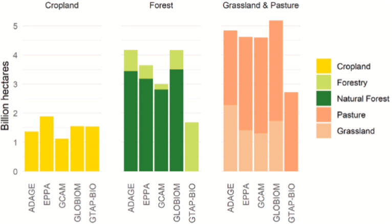
Estimates of induced LUC are sensitive to assumptions about which land is likely to convert in response to higher crop prices and the productivity of this land for producing crops. Replacing forests with cropland may release on average about four to five times more carbon emissions per unit land than converting pasture to cropland (Plevin et al., 2010), although there is wide variation in estimates. Melillo et al. (2009) show that allowing conversion of unmanaged natural areas to cropland leads to a seven-fold higher induced effect of biofuels compared to a scenario that only allows more intensive use of existing managed lands. The larger the potential for intensive management of land for biofuel feedstocks to displace other crops, the lower the induced land use effect of biofuels because it reduces extensive margin effects. A recent analysis of how models for assessing LUC treat availability of land showed how this parameter affects estimated CIs. Figure 9-1 provides a comparison of the different quantities of land categories available for conversion across a selection of models used for estimating biofuel-driven land use.

Price Responsiveness of Consumer Demand for Agricultural Commodities

The greater the elasticity of demand for agricultural commodities, the smaller the increase in crop prices due to the demand for biofuels and the smaller the resulting increase in land conversion to meet the additional demand for food crop-based biofuels.

Changes in Food Availability

Along with LUC, one of the consequences of increased competition for land due to biofuels could be a decrease in available food for consumption by humans. In a review of major models used to estimate market-mediated LUC, including GTAP-BIO (used by the California Air Resources Board), FAPRI-CARD (used by U.S. EPA), and MIRAGE (used by the European Union [EU]), Searchinger et al. (2015) found that the models resulted in decreased food availability for humans, the long-term GHG emissions consequences of which have gone largely unexplored, which is particularly important as global food demand is expected to increase substantially over the coming decades (Clark et al., 2020; Tilman et al., 2011). Further research is needed to assess the effect of biofuel production on food availability.

Ease of Transmission of Price Shocks in World Markets

The impact of increased biofuel production on LUCs in the rest of the world depends on the ease with which price shocks are transmitted from domestic markets to the rest of the world. This, in turn, depends on assumptions about the ease with which goods can be traded across countries. Some CGE models typically use the Armington approach⁵ which differentiates otherwise homogeneous goods by country of origin (Armington, 1969). Other CGE and all PE models assume that there is one world price for homogenous goods (an integrated world market) and goods will be produced where it is least costly to do so. These models allow for an easier transmission of a shock throughout the world economy which could result in “unrealistic” trade patterns. The Armington approach leads to results that follow observed trade patterns. A potential pitfall of this approach is that it allows price differentials for homogenous goods, such as imported ethanol and domestic ethanol, to persist. Estimates of the induced LUC effect are sensitive to the use of the Armington assumption as compared with the integrated world market assumption. With the Armington assumption in the GTAP-BIO model, land conversions are primarily concentrated in the United States and EU while with the integrated world market assumption they are more evenly distributed across the world and the share of global forest land converted to cropland is higher (Golub and Hertel, 2011).

Types of Biofuels

The mix and quantity of biofuels produced will affect the magnitude of the LUC caused by a low-carbon fuel policy. Low-carbon fuel policies can affect the mix of biofuels depending on the incentives they provide for biofuels from different feedstocks that differ in their CI, cost of production and other factors. This mix of biofuels and overall quantity will depend on the policy inducing the production of biofuels. The use of crop residues and high yielding dedicated energy crops may reduce the need for land for a given volume of biofuels compared to the use of food crops that have relatively lower yield. The overall ILUC intensity of a given target for biofuel consumption will depend on the mix of biofuels and the policy design, although it may not affect the feedstock specific LUC.

Size of the Biofuel Policy Shock

The induced LUC effect of a given target for biofuel consumption is likely to be scale and policy dependent. The magnitude of biofuel produced can affect the magnitude of the induced LUC due to nonlinearities in models (Laborde, 2011; Tyner et al., 2010). In CGE models, the concave shape of the constant elasticity of transformation function and the constant elasticity of substitution functions used to represent production possibilities and substitutability among consumption choices causes nonlinearity in effects. Additionally, non-linearity can also arise because the size of the policy shock and the type of policy can affect

___________________

⁵ The Armington assumption is that each country produces a distinct variety of a good. Some CGE models use an Armington elasticity to represent the elasticity of substitution for products from different countries or regions.

the mix of biofuels. The mix of policies can affect the indirect effect of a given volume of biofuel because they can change the mix and levels of different biofuels produced (Chen and Khanna, 2012; Laborde, 2011).

Time Horizon for Assessing the Land Use Change Effect

Induced LUC leads to the release of stored carbon in soils and vegetation if land is converted to crop production. To attribute these GHG emissions to each unit of biofuel produced and compare the induced emissions to the direct flow of carbon savings from using biofuels to displace fossil fuels, studies have amortized the induced LUC emissions over the time horizon that the land is expected to remain in crop production.

Conversion of Induced Land Use Changes to GHG Emissions

Assessing the effects of induced LUC on carbon emission requires two components: (1) An economic model to assess land use and land cover changes induced by biofuel production, or in the case of the approach of Searchinger et al. (2018) the land area used in production, and (2) a set of emissions factors to evaluate the potential emissions associated with each of land conversion or land type in production. Different methods for estimating effects of LUC attributable to biofuel production have been used. In the ALCA context, the opportunity cost of using land for biofuels has been explored with the development of a carbon benefits index that measures the relative output of land use of different types (Searchinger et al., 2018). While the existing literature has intensively discussed the land use modeling component, less attention has been paid to the implications of the choice of emission factors on the estimated ILUC values.

Conversion of Induced Land Use Changes to GHG Emissions

Assessing the effects of induced LUC on carbon emission requires two components: (1) An assessment of land use and land cover changes induced by biofuel production and (2) a set of emissions factors to evaluate the potential emissions associated with each of land conversion or land type in production. While the existing literature has intensively discussed the issue of assessing land use changes, less attention has been paid to the implications of the choice of emission factors on the estimated ILUC values.

The suitability, accuracy, and validity of the implemented emissions factors across the existing modeling efforts have not been reviewed extensively. The early papers in this field applied a set of land use emissions factors provided by the Woods Hole Research Center, Winrock International, or Intergovernmental Plan on Climate Change to estimate these emissions. Then a set of emissions factors developed by Gibbs et al. (2014) and Plevin et al. (2014) have been used in some studies. In support of its GREET model, Argonne National Laboratory developed a separate set of emissions factors (Kwon et al., 2020).⁶ Some modelers have developed their own emissions factors using the existing publications following the Intergovernmental Panel on Climate Change guidelines and its reference tables. The implemented emissions factors differ significantly across studies and are a major source of variation in land use emission estimates provided by various studies (Leland et al., 2018).

As models used to assess induced LUC have been updated over the last decade, they have incorporated new elements to reflect agricultural practices in finer detail, including multi-cropping, new land categories such as idled or marginal cropland, and new forms of market mediated responses to biofuel demand. It is worth noting at the beginning of this section that challenges with estimating the emissions consequences of market mediated LUC have led some researchers to call into question whether the modeling approaches described here can adequately quantify these emissions, even as such emissions are expected to occur (Daioglou et al., 2020; Malins et al., 2020). However, counter views have been presented by Taheripour et al. (2021).

___________________

⁶ This sentence was altered after the release of the pre-publication version of the report to the sponsor to acknowledge that Argonne National Laboratory developed a separate set of emissions factors.

Rebound Effect from Fossil Fuel Displacement

The rebound effect is also measured using economic models that include the domestic transportation sector, the global fuel sector and global trade in fossil fuels. These models include supply and demand relationships for fossil fuels and biofuels (or in some case vehicle miles travelled that are used to derive demand for alternative types of fuels) in domestic and global markets that are influenced by the biofuel policies. The extent to which these models cover the energy sector varies across the modeling practices. Some models only cover markets for ethanol and gasoline, while others cover a broader perspective including markets for fossil fuels across uses including but not limited to transportation and the link between the crude oil and refinery products. Estimates of the global rebound effect due to U.S. biofuels have varied substantially across studies depending on assumptions about the elasticity of supply of oil in the world market, market power in the oil market, and the quantity of biofuel produced. There are various determinants of the magnitude of the rebound effect, these include:

Market structure: Models differ in their assumption about the structure of the oil market. Some studies assume perfectly competitive markets with free trade in oil among countries. An alternative assumption is that there is sufficient market power in the oil market and that oil prices can be set by large oil producers in response to different market factors.

Elasticity of the world oil supply: Studies differ in their assumptions about the elasticity of world oil supply; this may depend on whether they are analyzing short term or long term effects. The more inelastic the supply curve the larger the reduction in world oil price in response to a reduction in biofuel induced demand for oil.

Elasticity of demand for fuel: The greater the elasticity of demand, the larger the reduction in demand for fuel due to a small policy induced increase in the price of fuel.

Comprehensiveness of fuel and energy markets: Studies differ in modeling the details of energy and fuel markets. A more comprehensive model provides a lower rebound effect.

Extent of trade in fuel with rest of the world: If the biofuel producing country is a small trader in oil then it is commonly assumed that, with a small open economy and a small amount of oil use, the effect on the global market will be negligible. If the biofuel producing country is a large trader in the world market, then it has greater potential to affect world price of oil assuming a competitive oil market (Chen et al., 2021).

Stringency of biofuel policy: The larger the biofuel mandate, the greater the need for displacing fossil fuel with biofuel and the larger the implicit penalty on fossil fuel use and implicit subsidy on biofuel use. This could have a larger negative effect on fossil fuel consumption and can lead to a larger rebound effect, depending on the various factors explained above.

Validation of Models Quantifying Indirect Land Use Change

As with any life-cycle model, since emissions due to LUC or fuel market effects that can be attributed to biofuels are not directly observable, the credibility of the estimates obtained depends on the quality of the model being used to quantify it. Validation of model outcomes by comparing the simulated outcomes with observed data is one approach for assessing the ability of models to predict realistic outcomes. Another approach to checking the credibility of the model is the extent to which the parametric assumptions of the model are supported by empirical evidence. Both of these approaches are however extremely difficult to implement. This is because the global models described above rely on a very large number of parameters and the empirical evidence for these parameters is often thin or not available at the spatial scale or for the time period most relevant for the model. Similarly, these models generate a very large number of numerical outcomes. While some of these may be close to observed data, others may not be; see Arndt et al. (2002) and Liu et al. (2004). The validation methodology offers no guidance on the acceptable deviation between observed and simulated outcomes and what constitutes a model as being valid or invalid. This is a subjective judgment similar to determining what constitutes a “reasonable” degree of uncertainty. Moreover, the time frame for model calibration or validation is typically shorter than the time frame over which predictions are to be made. Although the model may accurately reproduce observed data at a point in time, there is no assurance that it can perform equally well over a longer time frame. The effect of modeling uncertainties and errors on estimates of induced land use change are likely to be lower when one is comparing a difference (change) between two scenarios that hold all assumptions the same and only differ in the amount of biofuel produced. Despite the limitations of using models to make precise predictions, models serve a useful purpose of providing scientific understanding of the intended and unintended system-wide effects of a policy or technology change. Having a range of estimates from multiple models can create uncertainty but can also point to areas where there is greater consistency in findings and areas of large differences. This can be useful for policy design by showing the order of magnitude of effects.

As outlined above, validation of model results for future projections is not an easy task to accomplish. However, ex post validation is a more practical option. Models’ projections can be validated against new evidence and observation as time moves forward. Over the past 15 years various models have been used to evaluate the extent to which biofuel production could affect land use and LUCs. The results of these modeling practices vary widely. As discussed above, the existing literature shows a few key factors that explain most of the differences across models’ results: modeling yield improvement, the extent to which biofuel production occurs on the existing idled land or causes extensification, and the extent to which biofuel produced in one country affect land use changes in other countries due to trade. It is practical to assess the models’ assumptions on these key drivers and their land use projections and verify them according to the existing recent evidence. It may not be practical to assess all models’ parameters. However, after producing large quantities of biofuel in practice and having various observations, comparing hypothetical modeling projections with observations is a practical and valid practice and can help policy decision-making.

Inclusion of Market-Mediated Effects in Biofuel Policies

Policies to promote low-carbon fuels differ in the way in which they include induced effects in the CI of biofuels. The U.S. RFS specifies minimum thresholds for the CI of various types of biofuels, conventional, advanced and cellulosic, relative to conventional gasoline. For the RFS, the CI of a particular type of biofuel is the sum of a set of fuel supply chain emissions, emissions from induced agricultural practices, and induced LUC emissions intensity; together this sum needs to be lower than the threshold for that type of biofuel as assessed in 2022 to ensure compliance. The RFS regulatory impact assessment also estimated the 2012 and 2017 CI of biofuels, though the 2022 estimate was used to determine the categorization of biofuels within the policy. Uncertainty in estimates of induced LUC is dealt with by taking the mean value of the distribution of estimates of CIs.

In contrast with the RFS, the California Low Carbon Fuel Standard (CA-LCFS) requires specific estimates of the CI of a fuel pathway that can be compared with the goal of the policy (the desired CI of transportation fuel) in order to determine its compliance. The CA-LCFS determines the total CI of a biofuel by adding together the supply chain emissions intensity and induced LUC intensity of the biofuel.

Each of these policies uses an estimated ILUC factor for each type of biofuel that is treated to be invariant to scale of biofuel produced, time period or location of feedstock produced for that biofuel, within a country. To the extent that the ILUC effect is non-linearly related to the scale of production of a biofuel, this approach may under-estimate or over-estimate the magnitude of the effect. It also ignores potential circularity in the magnitude of the effect, since the scale of production depends on the deterrent effects of including the ILUC factor in determining compliance with the policy which in turn will influence the magnitude of the ILUC effect.

Precision in the specific estimate of CI of a biofuel can have meaningful implications for the fuel mix supplied under both an RFS and LCFS-like policy. For the purposes of the RFS, the CI can dictate which subcategory a fuel is eligible within, or its eligibility altogether, whereas in an LCFS a fuel’s estimated CI determines its compliance value within the policy. These policies ignore other types of indirect effects, such as those due to fuel market or livestock market effects. However, in the case of the CA-LCFS, the objective of including market-mediated effects in the CI of the biofuel is to deter (implicitly penalize) consumption of biofuels with large emissions from market-mediated effects and incentivize consumption of biofuels with lower total effects. However, the policy can still incentivize biofuels with higher relative ILUC emissions estimates if their total CI estimate is comparable to other fuels. A performance standard such as the CA-LCFS creates incentives to continuously reduce the CI of the low-carbon fuel over time and to substitute lower-CI biofuels for higher-CI biofuels, even within a type or across types, as compared to the RFS.

Since an LCFS is a CI standard, full compliance with it may achieve a reduction in CI (carbon emissions per unit fuel), but there is no guarantee that it will reduce the aggregate GHG emissions from the transportation sector. This will depend on the total volume of fuel consumed, which may offset more than the reduction in the CI of the fuel, and the degree to which the CI reflects the actual emissions attributable to the fuels. The increase in the volume of fuel use may occur for two reasons: a direct effect and an indirect effect. The direct effect arises because an LCFS implicitly penalizes the fuel with a CI higher than the standard and implicitly subsidizes the fuel with a CI lower than the standard. Depending on the magnitudes of these implicit taxes and subsidies, an LCFS can lower the overall cost of the blended transportation fuel and lead to greater demand for fuel. The indirect effect arises because the reduction in the demand for the high CI (fossil) fuels can lower market price of the fuel and lead to a rebound effect in the fuel market, as discussed above (see Holland et al., 2008; Khanna et al., 2014).

REFERENCES

Adler, P. R., S. J. Del Grosso, D. Inman, R. E. Jenkins, S. Spatari, and Y. Zhang. 2012. Mitigation opportunities for life-cycle greenhouse gas emissions during feedstock production across heterogeneous landscapes. In Managing Agricultural Greenhouse Gases 203–219, Elsevier.

Alakoski, E., M. Jämsén, D. Agar, E. Tampio, and M. Wihersaari, M. 2016. From wood pellets to wood chips, risks of degradation and emissions from the storage of woody biomass: A short review. Renewable and Sustainable Energy Reviews 54:376–383. https://doi.org/10.1016/j.rser.2015.10.021.

Alvarez, R. A., D. Z.- Araiza, D. R. Lyon, D. T. Allen, Z. R. Barkley, A. R. Brandt, K. J. Davis, S. P. Hamburg, S. C. Herndon, D. J. Jacob, A. Karion, E. A. Kort, B. K. Lamb, T. Lauvaux, J. D. Maasakkers, A. J. Marchese, M. Omara, S. W. Pacala, J. Peisch, A. L. Robinson, P. B. Shepson, C. Sweeney, A. Townsend-Small, and S. C. Wofsy. 2018. Assessment of methane emissions from the US oil and gas supply chain. Science 361(6398):186–188. https://www.science.org/doi/full/10.1126/science.aar7204.

Armington, P. S. 1969. A Theory of Demand for Products Distinguished by Place of Production (Une théorie de la demande de produits différenciés d’après leur origine) (Una teoría de la demanda de productos distinguiéndolos según el lugar de producción). Staff Papers (International Monetary Fund) 16(1):159–178. https://doi.org/10.2307/3866403.

Arndt, C., S. Robinson, and F. Tarp. 2002. Parameter estimation for a computable general equilibrium model: A maximum entropy approach. Economic Modelling 19:375–398.

Arora, S., M. Wu, and M. Wang. 2008. Update of Distillers Grains Displacement Ratios for Corn Ethanol Life-Cycle Analysis. ANL/ESD/11-1. Center for Transportation Research Energy Systems Division, Argonne National Laboratory. https://publications.anl.gov/anlpubs/2011/01/69222.pdf.

Astals, S., V. Nolla-Ardevol, and J. Mata-Alvarez. 2012. Anaerobic co-digestion of pig manure and crude glycerol at mesophilic conditions: Biogas and digestate. Bioresource Technology 110:63−70.

Baker, S. E., J. K. Stolaroff, G. Peridas, S. H. Pang, H. M. Goldstein, F. R. Lucci, W. Li, E. W. Slessarev, J. Pett-Ridge, F. J. Ryerson, and J. L. Wagoner. 2020. Getting to Neutral: Options for Negative Carbon Emissions in California. No. LLNL-TR-796100. Lawrence Livermore National Lab. (LLNL), Livermore, CA (United States); University of California, Berkeley, CA (United States); Negative Carbon Consulting, Half Moon Bay, CA (United States); University of Calgary, AB (Canada); University of Queensland, Brisbane, QLD (Australia); University of California, Davis, CA (United States); Worcester Polytechnic Institute, MA (United States); Georgetown University, Washington, DC (United States); Valence Strategic, Washington, DC (United States). https://www-gs.llnl.gov/content/assets/docs/energy/Getting_to_Neutral.pdf.

Beach, R. H. and B. A. McCarl. 2010. US Agricultural and Forestry Impacts of the Energy Independence and Security Act: FASOM Results and Model Description. Research Triangle Park, NC: RTI International. http://yosemite.epa.gov/Sab/Sabproduct.nsf/962FFB6750050099852577820072DFDE/$File/FASOM+Report_EISA_FR.pdf.

Booth, M.S. 2018. Not carbon neutral: Assessing the net emissions impact of residues burned for bioenergy. Environmental Research Letters 13(3):035001.

Bremer, V.R., A. J. Liska, T. J. Klopfenstein, G. E. Erickson, H. S. Yang, D. T. Walters, and K. G. Cassman. 2010. Emissions savings in the corn‐ethanol life cycle from feeding coproducts to livestock. Journal of Environmental Quality, 39(2):472-482.

Brentrup, F., J. Küsters J. Lammel and H. Kuhlmann. 2000. Methods to estimate on-field nitrogen emissions from crop production as an input to LCA studies in the agricultural sector. The International Journal of Life Cycle Assessment 5(6):349. https://doi.org/10.1007/BF02978670.

Breunig, H. M., J. Amirebrahimi, S. Smith, and C. D. Scown. 2019. Role of digestate and biochar in carbon-negative bioenergy. Environmental Science & Technology 53(22):12989−12998. https://pubs.acs.org/doi/abs/10.1021/acs.est.9b03763.

Cai, H., J. B. Dunn, Z. Wang, J. Han, and M. Q Wang. 2013. Life-cycle energy use and greenhouse gas emissions of production of bioethanol from sorghum in the United States. Biotechnology Biofuels 6:141 https://doi.org/10.1186/1754-6834-6-141.

Cai, H., J. Han, M. Wang, R. Davis, M. Biddy, and E. Tan. 2018. Life-cycle analysis of integrated biorefineries with co-production of biofuels and bio-based chemicals: Co-product handling methods and implications. Biofuels, Bioproducts and Biorefining 12(5):815−833. https://doi.org/10.1002/bbb.1893.

Campbell, R. M., N. M. Anderson, D. E. Daugaard, and H. T. Naughton. 2018. https://www.sciencedirect.com/science/article/pii/S0306261918312558.

CARB. 2017. Co-Processing of Biogenic Feedstocks in Petroleum Refineries: Draft Staff Discussion Paper. https://ww2.arb.ca.gov/sites/default/files/classic/fuels/lcfs/lcfs_meetings/020717_staffdiscussionpaper.pdf.

CARB. 2022. GHG Emissions and Sinks. https://www.epa.gov/ghgemissions/inventory-us-greenhouse-gas-emissions-and-sinks.

CARB. 2021. Inventory Data. https://ww2.arb.ca.gov/ghg-inventory-data.

Chambers, R.S., R. A. Herendeen, J. J. Joyce, and P. S. Penner. 1979. Gasohol: Does it or doesn’t it produce positive net energy? Science 206(4420):789−795. https://www.science.org/doi/10.1126/science.206.4420.789.

Chen, L., D. Debnath, J. Zhong, K. Ferin, A. VanLoocke, and M. Khanna, M. 2021. The economic and environmental costs and benefits of the renewable fuel standard. Environmental Research Letters 16(3):034021. https://doi.org/10.1088/1748-9326/abd7af.

Chen, X., Huang, H., Khanna, M., and Onal, H. 2014. Alternative Fuel Standards: Welfare Effects and Climate Benefits. Journal of Environmental Economics and Management 67:241–257.

Clark, M.A., N. G. Domingo, K. Colgan, S.K. Thakrar, D. Tilman, J. Lynch, I. L. Azevedo, and J. D. Hill. 2020. Global food system emissions could preclude achieving the 1.5 and 2 C climate change targets. Science, 370(6517):705-708.

Cowie, A. L., G. Berndes, N. S. Bentsen, M. Brandão, F. Cherubini, G. Egnell, B. George, L. Gustavsson, M. Hanewinkel, Z. M. Harris, and F. Johnsson. 2021. Applying a science‐based systems perspective to dispel misconceptions about climate effects of forest bioenergy. GCB Bioenergy 13(8):1210–1231. https://onlinelibrary.wiley.com/doi/epdf/10.1111/gcbb.12844.

Cruce, J. R. and J. C. Quinn. 2019. Economic viability of multiple algal biorefining pathways and the impact of public policies. Applied Energy 233:735–746.

Daioglou, V., G. Woltjer, B. Strengers, B. Elbersen, G. B. Ibañez, D. S. Gonzalez, J. G. Barno, and D. P. van Vuuren. 2020. Progress and barriers in understanding and preventing indirect land‐use change. Biofuels, Bioproducts and Biorefining 14(5):924–934.

Dumortier, J., H. Dokoohaki, A. Elobeid, D. J. Hayes, D. Laird, and F. E. Miguez. 2020. Global land-use and carbon emission implications from biochar application to cropland in the United States. Journal of Cleaner Production 258:120684. https://www.sciencedirect.com/science/article/pii/S0959652620307319#bib31.

Dumortier, J., D. J. Hayes, M. Carriquiry, F. Dong, X. Du, A. Elobeid, J. F. Fabiosa, and S. Tokgoz. 2011. Sensitivity of carbon emission estimates from indirect land-use change. Applied Economic Perspectives and Policy 33(3):428–48. https://doi.org/10.1093/aepp/ppr015.

European Commission. 2018. Phyllis: ECN Database of Biomass and Waste Properties.

Fabiosa, J. F., J. C. Beghin, F. Dong, A. Elobeid, S. Tokgoz, and T.-H. T.-H. Yu. 2010. Land Allocation Effects of the Global Ethanol Surge: Predictions from the International FAPRI Model. Land Economics 86(4):687–706.

Fargione, J., J. Hill, D. Tilman, S. Polasky, and P. Hawthorne. 2008. Land clearing and the biofuel carbon debt. Science 319:1235–8.

Favero, A., A. Daigneault and B. Sohngen. 2020. Forests: Carbon sequestration, biomass energy, or both? Science Advances 6(13):6792. https://www.science.org/doi/10.1126/sciadv.aay6792.

Flugge, M., Lewandrowski, J., Rosenfeld, J., Boland, C., Hendrickson, T., Jaglo, K., Kolansky, S., Moffroid, K., Riley-Gilbert, M. and Pape, D., 2017. A Life-Cycle Analysis of the Greenhouse gas emissions of corn-based ethanol. Report prepared by ICF under USDA Contract No. AG-3142-D-16-0243. January 12, 2017. https://digitalcommons.unl.edu/usdaarsfacpub/1617/

Gasparatos, A., P. Stromberg, and K. Takeuchi. 2013. Sustainability impacts of first-generation biofuels, Animal Frontiers 3(2):12–26. https://doi.org/10.2527/af.2013-0011.

Geronimo, C., S. E. Vergara, C. Chamberlin, and K. Fingerman. 2022. Overlooked emissions: Influence of environmental variables on greenhouse gas generation from woody biomass storage. Fuel 319(123839):0016–2361, https://doi.org/10.1016/j.fuel.2022.123839.

Gibbs, H. K., M. Johnston, J. A. Foley, T. Holloway, C. Monfreda, N. Ramankutty, and D. Zaks. 2008. Carbon payback times for crop-based biofuel expansion in the tropics: The effects of changing yield and technology. Environmental Research Letters 3(3):034001.

Gibbs, H., S. Yui, and R. J. Plevin. 2014. New Estimates of Soil and Biomass Carbon Stocks for Global Economic Models. GTAP Technical Paper No. 33. West Lafayette, Indiana: Purdue University.

Golub A. A., T. W. Hertel, and S. K. Rose. 2017. Global Land Use Impacts of U.S. Ethanol: Revised Analysis Using GDyn-BIO Framework. In Handbook of Bioenergy Economics and Policy: Volume II, M. Khanna, and D. Zilberman, eds. Natural Resource Management and Policy 40. Springer, New York, NY. https://doi.org/10.1007/978-1-4939-6906-7_8.

Golub, A. and T. W. Hertel. 2011. “Modeling Land Use Change Impacts of Biofuels in the GTAP-BIO Framework.” https://web.ics.purdue.edu/~hertel/data/uploads/publications/golub-hertel-climate-change-economics.pdf.

Gurgel, A., J. M. Reilly, and S. Paltsev. 2007. Potential Land Use Implications of a Global Biofuels Industry 36.

Hasler, K., S. Bröring, S. W. F. Omta, and H. W. Olfs. 2015. Life cycle assessment (LCA) of different fertilizer product types. European Journal of Agronomy 69:41–51. https://doi.org/10.1016/j.eja.2015.06.001. https://www.sciencedirect.com/science/article/pii/S1161030115000714.

Heijungs, R., K. Allacker, E. Benetto, M. Brandão, J. Guinée, S. Schaubroeck, T. Schaubroeck, and A. Zamagni. 2021. System Expansion and Substitution in LCA: A Lost Opportunity of ISO 14044 Amendment 2. Frontiers in Sustainability 2(40). https://doi.org/10.3389/frsus.2021.692055.

Hertel, T. W., W. E. Tyner, and D. K. Birur. 2010. The global impacts of biofuel mandates. Energy Journal 31(1):75–100.

Hill, J. 2022. “The sobering truth about corn ethanol.” PNAS 119:11. https://www.pnas.org/doi/10.1073/pnas.2200997119.

Hill, J., A. Goodkind, C. Tessum, S. Thakrar, D. Tilman, S. Polasky, T. Smith, N. Hunt, K. Mullins, M. Clark, and J. Marshall. 2019. Air-quality-related health damages of maize. Nature Sustainability 2:397–403. https://doi.org/10.1038/s41893-019-0261-y.

Hill, J., L. Tajibaeva and S. Polasky. 2016. Climate consequences of low-carbon fuels: The United States renewable fuel standard. Energy Policy 97:351–353. https://www.sciencedirect.com/science/article/pii/S0301421516303962?via%3Dihub.

Holland, S. P., J. E. Hughes, and C. R. Knittel. 2009. Greenhouse gas reductions under low carbon fuel standards? American Economic Journal: Economic Policy 1(1):106–46.

Hornafius, K. Y. and J. S. Hornafius. 2015. Carbon negative oil: A pathway for CO₂ emission reduction goals. International Journal of Greenhouse Gas Control 37:492–503. https://doi.org/10.1016/j.ijggc.2015.04.007.

Hsu, D. D. 2012. Life cycle assessment of gasoline and diesel produced via fast pyrolysis and hydroprocessing. Biomass and Bioenergy 45:41–47. https://doi.org/10.1016/j.biombioe.2012.05.019.

Huo, H., M. Wang, C. Bloyd, and V. Putsche. 2009. Life-cycle assessment of energy use and greenhouse gas emissions of soybean-derived biodiesel and renewable fuels. Environmental Science & Technology 43(3):750756. https://doi.org/10.1021/es8011436.

International Organization for Standardization. 2006. Environmental Management: Life Cycle Assessment; Requirements and Guidelines. ISO, Geneva.

International Standard Organization. 2020. ISO 14044:2006/AMD 2:2020 Environmental management — Life cycle assessment — Requirements and guidelines — Amendment 2. ISO.76, Geneva, Switzerland.

Ippolito, J. A., L. Cui, C. Kammann, N. Wrage-Mönnig, J. M. Estavillo, T. Fuertes-Mendizabal, M. L. Cayuela, G. Sigua, J. Novak, K. Spokas, and N. Borchard. 2020. Feedstock choice, pyrolysis temperature and type influence biochar characteristics: A comprehensive meta-data analysis review. Biochar 2:421–438. https://link.springer.com/article/10.1007/s42773-020-00067-x.

Joseph, S., Cowie, A. L., Van Zwieten, L., Bolan, N., Budai, A., Buss, W., Cayuela, M. L., Graber, E. R., Ippolito, J. A., Kuzyakov, Y., and Luo, Y. 2021. How biochar works, and when it doesn’t: A review of mechanisms controlling soil and plant responses to biochar. GCB Bioenergy 13(11):1731–1764.

Kauppi, P. E., P. Ciais, P. Högberg, P., A. Nordin, J. Lappi, T. Lundmark, and I. K. Wernick. 2020. Carbon benefits from Forest Transitions promoting biomass expansions and thickening. Global Change Biology 26(10):5365–5370. https://doi.org/10.1111/gcb.15292.

Keeler, B. L., B. J. Krohn, T. A. Nickerson, and J. D. Hill. 2013. US federal agency models offer different visions for achieving renewable fuel standard (RFS2) biofuel volumes. https://pubs.acs.org/doi/10.1021/es402181y.

Keeney, D. 2009. Ethanol USA. Environmental Science & Technology 43:8–11.

Khanna, M. and C. L. Crago. 2012. Measuring indirect land use change with biofuels: Implications for policy. Annual Review of Resource Economics 4(1):161–84. https://doi.org/10.1146/annurev-resource-110811-114523.

Khanna M., A. Ando and F. Taheripour. 2008. Welfare effects and unintended consequences of ethanol subsidies. Review of Agricultural Economics 30(3):411–421.

Khanna, M., L. Chen, B. Basso, X. Cai, J. L. Field, K. Guan, C. Jiang, T. J. Lark, T. L. Richard, S. A. Spawn‐Lee, and P. Yang. 2021. Redefining marginal land for bioenergy crop production. GCB Bioenergy 13(10):1590–1609. https://onlinelibrary.wiley.com/doi/10.1111/gcbb.12877.

Khanna, M., P. Dwivedi and R. Abt. 2017. Is Forest. Bioenergy Carbon Neutral or Worse than Coal? Implications of Carbon Accounting Methods. International Review of Environmental and Resource Economics 10(3–4):299–346.

Khanna, M., D. Rajagopal and D. Zilberman. 2021. Lessons learned from US experience with biofuels: Comparing the hype with the evidence. Review of Environmental Economics and Policy 15(1):67–861.

Khanna, M., W. Wang, T. Hudiburg, and E. DeLucia. 2017. The social inefficiency of regulating indirect land use change due to biofuels. Nature Communications 8:15513.

Khanna, M., D. Zilberman, and C. Crago. 2014. Modeling Land Use Change with Biofuels. In The Oxford Handbook of Land Economics. Oxford University Press, Oxford, UK.

Kim, S., X. Zhang, A. D. Reddy, B. E. Dale, K. D. Thelen, C. D. Jones, R. C. Izaurralde, T. Runge, and C. Maravelias. 2020. Carbon-negative biofuel production. Environmental Science & Technology 54(17):10797–10807. https://doi.org/10.1021/acs.est.0c01097.

Klein, D., C. Wolf, C. Schulz, and G. Weber-Blaschke. 2015. 20 years of life cycle assessment (LCA) in the forestry sector: State of the art and a methodical proposal for the LCA of forest production. International Journal of Life Cycle Assessment 20:556–575. https://doi.org/10.1007/s11367-015-0847-1.

Knapp, E. E., A. A. Bernal, J. M. Kane, C. J. Fettig, and M. P. North. 2021. Variable thinning and prescribed fire influence tree mortality and growth during and after a severe drought. Forest Ecology and Management 479:118595. https://doi.org/10.1016/j.foreco.2020.118595.

Kwon, H., X. Liu, J. B. Dunn, S. Mueller, M. M. Wander, and M. Wang. 2020. Carbon Calculator for Land Use and Land Management Change from Biofuels Production (CCLUB). Argonne National Laboratory, ANL/ESD/12–5, Rev.6.

Laborde, D. and H. Valin. 2012. Modeling land-use changes in a global CGE: Assessing the EU biofuel mandates with the MIRAGE-BioF model. Climate Change Economics 3(3):1250017. https://doi.org/10.1142/S2010007812500170.

Lammens, T. M. 2020. Methodologies for biogenic carbon determination when co-processing fast pyrolysis bio-oil. Energy Conversion and Management: X, 10, 100069. https://doi.org/10.1016/j.ecmx.2020.100069.

Lan, K., L. Ou, S. Park, S. S. Kelley, P. Nepal, H. Kwon, H. Cai, and Y. Yao. 2021. Dynamic life-cycle carbon analysis for fast pyrolysis biofuel produced from pine residues: implications of carbon temporal effects. Biotechnology for Biofuels and Bioproducts 14:191. https://doi.org/10.1186/s13068-021-02027-4.

Lan, K., L. Ou, S. Park, S. S. Kelley, and Y. Yao. 2020. Life cycle analysis of decentralized preprocessing systems for fast pyrolysis biorefineries with blended feedstocks in the southeastern United States. Energy Technology 8(11):1900850. https://doi.org/10.1002/ente.201900850.

Lan, K., L. Ou, S. Park, S. S. Kelley, B. C. English, E. T. Yu, J. Larson, and Y. Yao. 2021. Techno-economic analysis of decentralized preprocessing systems for fast pyrolysis biorefineries with blended feedstocks in the southeastern United States. Renewable and Sustainable Energy Reviews 143:110881. https://doi.org/https://doi.org/10.1016/j.rser.2021.110881.

Lan, K., S. S. Kelley, P. Nepal, and Y. Yao. 2020. Dynamic life cycle carbon and energy analysis for cross-laminated timber in the Southeastern United States. Environmental Research Letters.

Lark, T. J., N. P. Hendricks, A. Smith, N. Pates, S. A. Spawn-Lee, M. Bougie, E. G. Booth, C. J. Kucharik, and H. K. Gibbs. 2022. Environmental outcomes of the US Renewable Fuel Standard. Proceedings of the National Academy of Sciences 119(9):e2101084119.

Lawrence, N. C., C. G. Tenesaca, A. VanLoocke, and S. J. Hall. 2021. Nitrous oxide emissions from agricultural soils challenge climate sustainability in the US Corn Belt. Proceedings of the National Academy of Sciences, 118(46), e2112108118. https://doi.org/10.1073/pnas.2112108118.

Lee, U., Z. Lu, P. Su, M. Wang, V. DaVita, and D. Collings. 2022. Carbon Intensities of Refining Products in Petroleum Refineries with Co-processed Biofeedstocks. Argonne National Laboratory. ANL/ESD-21/20 https://publications.anl.gov/anlpubs/2022/02/173380.pdf.

Lee, E. K., X. Zhang, P. R. Adler, G. S. Kleppel, and X. X. Romeiko. 2020. Spatially and temporally explicit life cycle global warming, eutrophication, and acidification impacts from corn production in the US Midwest. Journal of Cleaner Production 242:118465. https://www.sciencedirect.com/science/article/abs/pii/S0959652619333359.

Lehmann, J., A. Cowie, C. A. Masiello, C. Kammann, D. Woolf, J. E. Amonette, M. L. Cayuela, M. CampsArbestain, and T. Whitman. 2021. Biochar in climate change mitigation. Nature Geoscience 14(12):883–892.

Leland, S., S. K. Hoekman, and X. Liu. 2018. “Review of modifications to indirect land use change modeling and resulting carbon intensity values within the California Low Carbon Fuel Standard regulations.” Journal of LCeaner Production 180:698-707. https://doi.org/10.1016/j.clepro.2018.01.077.

Lewandrowski, J., J. Rosenfeld, D. Pape, T. Hendrickson, K. Jaglo, and K. Moffroid, K. 2020. The greenhouse gas benefits of corn ethanol: Assessing recent evidence. Biofuels 11(3):361–375. https://doi.org/10.1080/17597269.2018.1546488.

Linger, J. G., D. R. Vardon, M. T. Guarnieri, E. M. Karp, G. B. Hunsinger, M. A. Franden, C. W. Johnson, G. Chupka, T. J. Strathmann, P. T. Pienkos, and G. T. Beckham. 2014. Lignin valorization through integrated biological funneling and chemical catalysis. Proceedings of the National Academy of Sciences 111.33:12013–12018. https://doi.org/10.1073/pnas.1410657111.

Liu, J., C. Arndt and T. W. Hertel. 2004. Parameter estimation and measures of fit in a global, general equilibrium model. Journal of Economic Integration 19(3):626–649.

Liu, W., Z. Zhang, X. Xie, Z. Yu, K. von Gadow, J. Xu, S. Zhao, and Y. Yang. 2017a. Analysis of the global warming potential of biogenic CO₂ emission in life cycle assessments. Scientific Reports 7:39857. https://doi.org/10.1038/srep39857.

Liu, W., Z. Yu, X. Xie, K. V. Gadow, and C. Peng. 2017b. A critical analysis of the carbon neutrality assumption in life cycle assessment of forest bioenergy systems. Environmental Reviews 26(1):93–101. https://doi.org/10.1139/er-2017-0060.

Liu, X., H. Kwon and M. Wang. 2021. Varied farm-level carbon intensities of corn feedstock help reduce corn ethanol greenhouse gas emissions. Environmental Research Letters 16(6):064055. https://iop-science.iop.org/article/10.1088/1748-9326/ac018f.

Maestrini, B. and B. Basso. 2018. Drivers of within-field spatial and temporal variability of crop yield across the US Midwest. Scientific Reports 8:14833. https://doi.org/10.1038/s41598-018-32779-3.

Malins, C., R. Plevin and R. Edwards. “How robust are reductions in modeled estimates from GTAP-BIO of the indirect land use change induced by conventional biofuels?” Journal of Cleaner Production 258:120716. doi:10.1016/j.clepro.2020.120716.

Markewitz, D. 2006. Fossil fuel carbon emissions from silviculture: Impacts on net carbon sequestration in forests. Forest Ecology and Management 236(2):153–161. https://doi.org/10.1016/j.foreco.2006.08.343.

Maroušek, J., M. Vochozka, J. Plachý and J. Žák. 2017 Glory and misery of biochar. Clean Technologies and Environmental Policy, 19, 311–317. https://link.springer.com/article/10.1007/s10098-016-1284-y.

McEwan, A., Brink, M., and Spinelli, R. 2019. Efficiency of Different Machine Layouts for Chain Flail Delimbing, Debarking and Chipping. Forests 10(2):126. https://www.mdpi.com/1999-4907/10/2/126.

Melilio, J. M., P. A. Steudler, J. D. Aber, K. Newkirk, H. Lux, F. P. Bowles, C. Catricala, A. Magill, T. Ahrens, and S. Morrisseau. 2002. “Soil Warming and Carbon-Cycle Feedbacks to the Climate System.” Science 298(2173). https://doi.org/10.1126/science.1074153.

Moset, V., M. Poulsen, R. Wahid, O. Højberg, and H. B. Møller. 2015. Mesophilic versus thermophilic anaerobic digestion of cattle manure: Methane productivity and microbial ecology. Microbial Biotechnology 8(5):787−800.

National Renewable Energy Laboratory (NREL). 2012. U.S. Life Cycle Inventory Database.

Nie, Y. and X. Bi. 2018. Life-cycle assessment of transportation biofuels from hydrothermal liquefaction of forest residues in British Columbia. Biotechnology for Biofuels 11(1):23. https://doi.org/10.1186/s13068-018-1019-x.

Lan, K., S. Park, and Y. Yao. 2019. “Key issue, challenges, and status quo of models for biofuel supply chain design.” In: Biofuels for a More Sustainable Future: Life Cycle Sustainability Assessment and Multi-Criteria Decision Making. Biofuels for a More Sustainable Future: Life Cycle Sustainability Assessment and Multi-Criteria Decision Making. pp. 273-315. https://doi.org/10.1016/B978-0-12-815581-3.00010-5.

Oneil, E. E., L. R. Johnson, B. R. Lippke, J. B. McCarter, M. E. McDill, P. A. Roth, and J. C. Finley. 2010. Life-cycle impacts of inland northwest and northeast/north central forest resources. Wood and Fiber Science 42:29−51.

Pingoud, K., T. Ekholm, R. Sievänen, S. Huuskonen, and J. Hynynen. 2018. Trade-offs between forest carbon stocks and harvests in a steady state: A multi-criteria analysis. Journal of Environmental Management 210:96−103. https://www.sciencedirect.com/science/article/pii/S0301479717312641?via%3Dihub.

Plevin, R. J., J. Jones, P. Kyle, A. W. Levy, M. J. Shell and D. J. Tanner. 2022. Choices in Land Representation Materially Affect Modeled Biofuel Carbon Intensity Estimates. Journal of Cleaner Production 349:131477. https://doi.org/10.1016/j.jclepro.2022.131477.

Plevin, R., H. Gibbs, J. Duffy, S. Yui, and S. Yeh. 2014. Agro-ecological Zone Emission Factor (AEZEF) Model (V47), GTAP Technical Paper No. 34. West Lafayette, Indiana: Purdue University.

Pognani, M., G. D’Imporzano, B. Scaglia, and F. Adani. 2009. Substituting energy crops with organic fraction of municipal solid waste for biogas production at farm level: A full-scale plant study. Process Biochemistry 44(8):817−821.

Powlson, D. S., M. J. Glendining, K. Coleman, and A. P. Whitmore. 2011. Implications for Soil Properties of Removing Cereal Straw: Results from Long‐Term Studies 1. Agronomy Journal. https://doi.org/10.2134/agronj2010.0146s.

Qin, Z., C. E. Canter, J. B. Dunn, S. Mueller, H. Kwon, J. Han, M. M. Wander, and M. Wang. 2018. Land management change greatly impacts biofuels’ greenhouse gas emissions. GCB Bioenergy 10(6):370−381.

Robertson, G. P., V. H. Dale, O. C. Doering, S. P. Hamburg, J. M. Melillo, M. M. Wander, W. J. Parton, P. R. Adler, J. N. Barney, R. M. Cruse, and C. S. Duke. 2008. Sustainable biofuels redux. Science 322(5898):49–50.

Sahoo, K., E. M. Bilek, and S. Mani. 2018. Techno-economic and environmental assessments of storing woodchips and pellets for bioenergy applications. Renewable and Sustainable Energy Reviews 98:27–39. https://doi.org/10.1016/j.rser.2018.08.055.

Salkuyeh, Y. K., B. A. Saville, and H. L. MacLean. 2018. Techno-economic analysis and life cycle assessment of hydrogen production from different biomass gasification processes. International Journal of Hydrogen Energy 43(20):9514–9528. https://doi.org/10.1016/j.ijhydene.2018.04.024.

Sanchez, D. L., N. Johnson, S. T. McCoy, P. A. Turner, and K. J. Mach. 2018. Near-term deployment of carbon capture and sequestration from biorefineries in the United States. Proceedings of the National Academy of Sciences 115(19):4875–4880. https://doi.org/10.1073/pnas.1719695115.

Sathaye, J., O. Lucon, A. Rahman, J. Christensen, F. Denton, J. Fujino, G. Heath, M. Mirza, H. Rudnick, and A. Schlaepfer. 2011. Renewable Energy in the Context of Sustainable Development. IPCC Special Report on Renewable Energy Sources and Climate Change Mitigation.

Schmidt, J. H., B. P. Weidema, and M. Brandão. 2015. A framework for modelling indirect land use changes in life cycle assessment. Journal of Cleaner Production 99(0959–6526):230–238.

Scown, C. D., W. W. Nazaroff, U. Mishra, B. Strogen, A. B. Lobscheid, E. Masanet, N. J. Santero, A. Horvath, and T. E. McKone. 2012. Lifecycle greenhouse gas implications of US national scenarios for cellulosic ethanol production. Environmental Research Letters 7(1):014011. https://doi.org/10.1088/1748-9326/7/1/014011.

Searchinger, T., R. Edwards, D. Mulligan, R. Heimlich, and R. Plevin. 2015. Do biofuel policies seek to cut emissions by cutting food? Science 347(6229):1420–1422.

Searchinger, T., R. Heimlich, R. A. Houghton, F. Dong, A. Elobeid, J. Fabiosa, S. Tokgoz, D. Hayes and T.-H Yu. 2008. Use of U.S. croplands for biofuels increases greenhouse gases through emissions from land-use change. Science 319(5867):1238–1240. https://doi.org/10.1126/science.1151861.

Shakoor, A., S. Shakoor, A. Rehman, F. Ashraf, M. Abdullah, S. M. Shahzad, T. H. Farooq, M. Ashraf, M. A. Manzoor, M. M. Altaf, and M. A. Altaf. 2021. Effect of animal manure, crop type, climate zone, and soil attributes on greenhouse gas emissions from agricultural soils—A global meta-analysis, Journal of Cleaner Production 278(124019):0959–6526. https://doi.org/10.1016/j.jclepro.2020.124019.

Sikarwar, V. S., M. Zhao, P. S. Fennell, N. Shah, and E. J. Anthony. 2017. Progress in biofuel production from gasification. Progress in Energy and Combustion Science 61:189–248. https://doi.org/10.1016/j.pecs.2017.04.001.

Sitepu, I. R., L. A. Garay, R. Sestric, D. Levin, D. E. Block, J. B. German, and K. L. Boundy-Mills. 2014. Oleaginous yeasts for biodiesel: Current and future trends in biology and production.” Biotechnology Advances 32(7):1336–1360.

Smith, T. M., A. L. Goodkind, T. Kim, R. E. O. Pelton, K. Suh, and J. Schmitt. 2017. Subnational Mobility and Consumption-Based Environmental Accounting of US Corn in Animal Protein and Ethanol Supply Chains. PNAS.

Spatari, S., Y. Zhang, and H. L. MacLean. 2005. Life cycle assessment of switchgrass-and corn stover-derived ethanol-fueled automobiles. Environmental Science & Technology 39(24):9750–9758. https://doi.org/10.1021/es048293.

Susmozas, A., D. Iribarren, P. Zapp, J. Linβen, and J. Dufour. 2016. Life-cycle performance of hydrogen production via indirect biomass gasification with CO₂ capture. International Journal of Hydrogen Energy 41(42):19484–19491. https://doi.org/10.1016/j.ijhydene.2016.02.053.

Taheripour, F. and W. Tyner. 2014. Welfare Assessment of the Renewable Fuel Standard: Economic Efficiency, Rebound Effect, and Policy Interactions in a General Equilibrium Framework. In Modeling, Optimization and Bioeconomy, A. Pinto and D. Zilberman, eds.

Taheripour, F., X. Zhao, and W. E. Tyner. 2017. The Impact of Considering Land Intensification and Updated Data on Biofuels Land Use Change and Emissions Estimates. Biotechnology for Biofuels 10(1):191. https://doi.org/10.1186/s13068-017-0877-y.

Taptich, M. N., C. D. Scown, K. Piscopo, and A. Horvath. 2018. Drop-in biofuels offer strategies for meeting California’s 2030 climate mandate. Environmental Research Letters, 13(9):094018. https://doi.org/10.1088/1748-9326/aadcb2.

Tilman, D., J. Hill and C. Lehman. 2006. Carbon-negative biofuels from low-input high-diversity grassland biomass. Science 314(5805):1598–1600.

Tilman, D., R. Socolow, J. Foley, J. Hill, E. Larson, L. Lynd, S. Pacala, J. Reilly, T. Searchinger, C. Somerville, and R. Williams. 2009. Beneficial biofuels – The food, energy, and environment trilemma. Science 32:270–271.

Tu, Q., M. Eckelman, and J. Zimmerman. 2017. Meta-analysis and harmonization of life cycle assessment studies for algae biofuels. Environmental Science & Technology 51(17):9419–9432.

Tyner, W. and F. Taheripour. 2007. Renewable Energy Policy Alternatives for the Future. American Journal of Agricultural Economics 89(5):1303–1310.

Tyner, W. and F. Taheripour. 2014. Advanced Biofuels: Economic Uncertainties, Policy Options, and Land Use Impacts. In Plants and Bioenergy, B. McCann, and Carpita, eds. Advances in Plant Biology, Vol. 4, Springer Science+Business Media, New York.

Verkerk, P. J., I. M. De Arano, and M. Palahí. 2018. The bio-economy as an opportunity to tackle wildfires in Mediterranean forest ecosystems. Forest policy and economics 86:1–3.

Wang, C., B. Amon, K. Schulz, and B. Mehdi. 2021. Factors that influence nitrous oxide emissions from agricultural soils as well as their representation in simulation models: A review. Agronomy 11:770. https://doi.org/10.3390/agronomy11040770.

Weidema, B. P., Ch. Bauer, R. Hischier, Ch. Mutel, T. Nemecek, J. Reinhard, C. O. Vadenbo, and G. Wernet. 2013. The Ecoinvent Database: Overview and Methodology, Data Quality Guideline for the Ecoinvent Database Version 3.

Whittaker, C., N. E. Yates, S. J. Powers, N. Donovan, T. Misselbrook, and I. Shield. 2017. Testing the use of static chamber boxes to monitor greenhouse gas emissions from wood chip storage heaps. BioEnergy Research 10(2):353–362. https://doi.org/10.1007/s12155-016-9800-9.

Wihersaari, M. 2005. Evaluation of greenhouse gas emission risks from storage of wood residue. Biomass and Bioenergy 28(5):444–453. https://doi.org/10.1016/j.biombioe.2004.11.011.

Woolf, D. and J. Lehmann. 2012. Modelling the long-term response to positive and negative priming of soil organic carbon by black carbon. Biogeochemistry 111(1−3):83−95.

Yang, M. N. R. Baral, A. Anastasopoulou, H. M. Breunig, and C. D. Scown. 2020. Cost and life-cycle greenhouse gas implications of integrating biogas upgrading and carbon capture technologies in cellulosic biorefineries. Environmental Science & Technology 54 (20): 12810-12819. https://doi.org/10.1021/acs.est.0c02816.

REFERENCES

Achat, D. L., C. Deleuze, G. Landmann, N. Pousse, J. Ranger, and L. Augusto. 2015. Quantifying consequences of removing harvesting residues on forest soils and tree growth – A meta-analysis. Forest Ecology and Management 348:124–141. https://doi.org/10.1016/j.foreco.2015.03.042.