
5.1 INTRODUCTION
Once oil has entered the marine environment, its chemical composition, physical properties, and behavior immediately begins to change due to combinations of dynamic processes that ultimately determine the fate of its components over time. Various combinations of processes dominate in different circumstances and locations in the marine ecosystem, discussed in detail in this chapter (see Figure 5.1). The aggregate of these processes determines the fate of oil and its diverse components, including the transport of bulk oil from one marine compartment to another (e.g., moving from a surface slick to dispersion in the water column or stranding on the shoreline), transformation of oil components to partially oxidized products (e.g., by photo-oxidation or biodegradation), and/or selective removal of oil components from the ocean (e.g., by volatilization or biodegradation). It should be clear that the “ultimate fate” of oil is dependent on time, as the processes described below act over time spans of hours (e.g., evaporation) to geological time (e.g., burial in sediments) and affect different proportions of different oils, ranging from minor changes to residual oil (e.g., ultra-heavy oils) to nearly complete removal from the ocean (e.g., jet fuel).
5.1.1 Major Advances in the Past 20 Years
Since publication of Oil in the Sea III report (NRC, 2003) there have been major technological advances in our ability to monitor and predict the fates of spilled oil in the ocean. In the previous report the chapter describing the behavior and fate of oil focused on physico-chemical weathering of spilled oil, including transport mechanisms, primarily at or near the surface. With the exception of photo-oxidation, our understanding of these fundamental processes has not changed substantially since then, yet our appreciation of how these processes work and how to predict them has improved substantially. The past two decades have provided tremendous advances in analytical methodology for detection and identification of oil constituents and their oxidized products (reviewed in Chapter 2), enabling sophisticated tracking, monitoring and forensic identification of spilled oil. Research into the Deepwater Horizon (DWH) spill provided additional information about the fate of subsurface spills, use of subsurface dispersant injection, modeling of gas-oil mixtures at depth, and behavior of oil plumes in deep waters. Whereas the 2003 report did not thoroughly examine biodegradation as a fate of spilled oil, extraordinary technological and conceptual advances made in analysis of microbial communities in the ocean (‘omics techniques) were buoyed by broad progress in DNA sequencing and bioinformatic software development and applied to research into the DWH spill. Furthermore, anaerobic hydrocarbon biodegradation pathways, which were not considered in the previous report, have been increasingly recognized as the major fate of oil sequestered in anaerobic marine sediments. These biological/biochemical advances, combined with the analytical chemistry developments, have taken marine oil spill research into the realm of “big data.” In addition to technological advances, there have been surprising insights into important processes associated with the fate of marine oil spills that arose from the DWH spill, including recognition of the importance of photooxidation and the large-scale but transient role of marine oil snow sedimentation and flocculant accumulation (MOSSFA) in oil removal and sedimentation, described in this chapter. In parallel, significant advances have been made in understanding the formation and transport of oil:mineral aggregates in the near-shore and on beaches. The DWH spill was also a driver for refining models of bubble and droplet formation
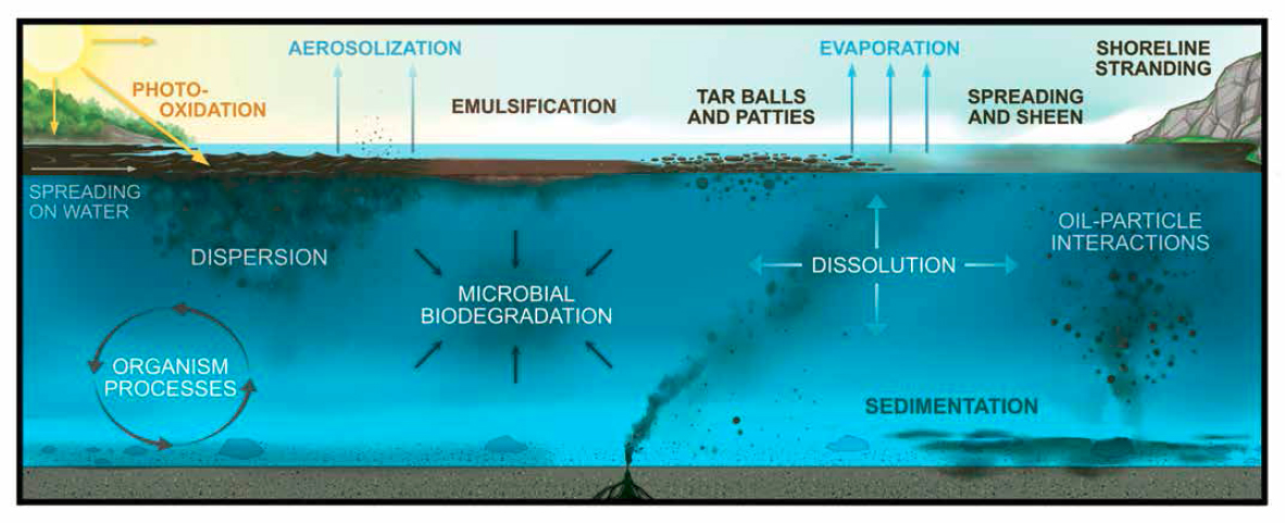
SOURCE: Image provided courtesy of the American Petroleum Institute, produced by Iron Octopus Productions, Inc.
and understanding the consequences of subsurface dispersant injection. Finally, the previous report concentrated on continental U.S. waters, whereas there is increased concern about oil spills in cold regions; the current chapter describes recent advances into the fate of oil in Arctic marine environments, particularly interactions of oil and ice.
5.1.2 Chapter Structure and Caveats
This chapter will convey to the reader the myriad interacting processes that affect the transport, transformation and ultimate fates of oil components, and emphasize the complexity of spill modeling. However, it is important that the reader appreciates some limitations to understanding, monitoring, and predicting the fate of oil in the sea. Three caveats in particular are noteworthy. (1) As Figure 5.1 suggests, at any given marine location there potentially are numerous interacting processes that can transport and transform oil over broad timespans. Each spill is unique because most oils are themselves unique and furthermore change dynamically over time in the diverse marine environments that they impact. Responders quip that they can “never respond to the same spill twice” because each individual spill is idiosyncratic and the processes affecting it are constantly changing, and because different spills experience unique combinations of processes in different parts of their impacted ecosystem. (2) Observing and measuring the fate of oil in the sea requires repeated sampling over time and in geographical space. This can be more difficult than it sounds because the marine environment is heterogeneous over many size and time scales, from micrometer-sized oil droplets in millimeter-sized pore spaces in beach sand to many square miles of evaporating oil slick on the water surface. Sampling a water column at exactly the same geographical location and depth on successive days may reveal very different oil concentrations, depending on where the currents, tides, eddies, wind, and so forth have transported the oil. Some sample variation might be overcome by exhaustive sampling, but that may challenge analytical capacity and be very expensive. Therefore, observing, modeling, and predicting the fate of oil in a specific situation requires inexact (but experienced) extrapolation from previous oil spill observations and from literature describing laboratory research. (3) Laboratory experiments can provide guidance for predicting oil fates in the field but, unfortunately, some of the published literature is based on experimental conditions that, while academically interesting, do not scale up to actual oil spills. For example, sometimes the type of oil tested or its experimental concentration are inappropriate; or the experimental conditions do not capture field parameters due to difficulty simulating natural processes in the laboratory (e.g., tidal action, mixing by wind and wave energy, oil leaking from sunken wrecks [see Box 3.6] ambient pressure and biological activity rather than high hydrostatic pressure, lack of solar radiation, and so on); sometimes the experimental time scale is too short to capture meaningful data on long-term fates; and sometimes the experimental biota within the test are inappropriate, having been cultivated in the laboratory rather than collected from the spill site, or are incubated with nutrients at concentrations not found in the ocean. In fact, it is difficult even for experts to define “environmentally relevant experimental conditions” (see Chapter 6, Box 6.4), given the first two caveats on dynamics and heterogeneity. Nevertheless, these limitations fundamentally influence calculation of oil budgets (see Section 5.2.9), modeling of oil spill fates (see Section 5.5), and monitoring of oil spills (see Chapter 4).
With these limitations in mind, the descriptions of processes in this chapter, assembled from a combination of laboratory and field measurements, summarize our best current understanding of the fates of oil in the sea. Section 5.2 is an overview of the fundamental physical, chemical, and biological processes and reactions that influence the fate of oil in the marine environment, regardless of specific geographical location and oil type. It also provides examples of “spill budgets” that estimate the proportional fates of spilled oil. Section 5.3 discusses the fates of episodic oil spills (typically from a single, finite event) in specific marine systems, from surface and near-surface waters, through the water column to deep water and deep-sea sediments, along shorelines including beaches and estuaries, and describing the fate of oil in Arctic conditions as a special case. Section 5.4 describes the fates of oil from continuing (“chronic”) oil inputs, where their typically lower concentrations and more diffuse sources impact the relevant fate processes in important ways. Section 5.5 summarizes the uses of oil spill models for predicting the fates of marine oil spills. Section 5.6 summarizes conclusions and research needs arising from the literature review. Studies conducted during and after the DWH oil spill generated enormous amounts of information about the fate of Macondo 252 oil in the Gulf of Mexico; highlights of this research are integrated throughout the chapter without allowing this wealth of literature to dominate the knowledge and research needs of the broader marine environment. Notably, research and assessment of smaller spills in U.S. waters and elsewhere in the world also have contributed to advancing our knowledge of oil fates relevant to the focus of this chapter and the Statement of Task for this report.
5.2 FUNDAMENTAL TRANSPORT AND WEATHERING PROCESSES
This section provides an overview of the physico-chemical and biological processes that affect oil in the sea, regardless of geography and oil type. It describes the different states of oil and gas, formation of bubbles and droplets in water, transport in the ocean environment, volatilization of hydrocarbons to the atmosphere, photo-oxidation at the ocean surface, dissolution of hydrocarbons into water, emulsification of oil in water and water in oil, biodegradation fundamentals and the interactions of these processes. For context, Figure 5.2 illustrates the relative persistence of oil fractions in the
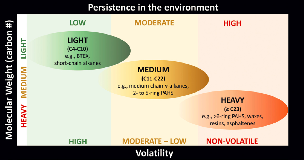
environment, which is affected by the fate processes summarized in Box 5.1 and Table 5.1 and described throughout this chapter.
5.2.1 Phases and States of Petroleum Fluids in the Sea
As discussed in detail in Section 2.2, petroleum may occur in the natural environment as a solid, liquid, or gas. In this section, we focus on liquid and gas as these are the most common forms of petroleum in the marine environment. Oil and gas properties depend on the composition of the petroleum fluid and on the thermodynamic state, normally defined by a given temperature and pressure. Following the approach in Chapter 2, we define standard conditions in this chapter following the Society of Petroleum Engineers (SPE), with standard temperature given as 15°C and standard pressure at 100 kilopascal (kPa).
Several important terms describing petroleum states and the various stages of transformation will be used in this chapter. As explained in Section 2.2, mixtures of liquid- and gas-phase petroleum may be in thermodynamic equilibrium within the petroleum reservoir, with a large fraction of the low molecular weight compounds dissolved in the liquid oil. As these fluids are released, either naturally through seeps, purposefully during production, or accidentally in an oil spill, the temperature and pressure of these fluids may change, possibly resulting in their phase and composition change. Liquid oil or gas at equilibrium in the reservoir or at equilibrium or disequilibrium with any state other than standard conditions is considered to be live oil and live gas, the term “live” indicating that the composition would evolve if brought to standard conditions, usually by release of gaseous compounds still dissolved in the liquid-phase oil. Likewise, dead oil refers to liquid petroleum that has released enough of the dissolved gases that it is in equilibrium with its gaseous headspace at standard conditions. Dead oil still contains some of its volatile components. Because the oil and gas from the DWH oil spill was emitted as a live mixture, oil spill science now recognizes the important implications of the live oil state, and significant new research has been conducted at a wide range of temperatures and pressures to understand the interactions of live oil and gas with the sea. Weathered oil is used to describe a petroleum liquid that has an altered composition from that with which it was released. Numerous processes alter the composition of petroleum fluids, and these are the topics of this chapter. We use the term weathering to refer generally to any process that alters the composition of oil or gas in the environment; we will also refer to many specific weathering processes by their various names, for example, dissolution, biodegradation, and photo-oxidation.
Because we commonly refer to liquid-phase petroleum as oil, we use this term throughout the report wherever it is not ambiguous. When the particular phase of matter must be specified for clarity, we will use the terms liquid oil or liquid petroleum. Some petroleum compounds are also commonly
referred to as gases because they are in the gas phase at standard conditions, for example, methane. We will likewise refer to these compounds as gases, specifying their state only if they are present in the liquid phase, as may occur at low temperature and high pressure. For more details about the states and compositions of petroleum fluids, see Chapter 2.
5.2.2 Immiscible Dynamics of Oil and Gas in Seawater: Sheens, Slicks, Bubbles, and Droplets
Spilled oil and gas interact with the marine environment through their immiscible interfaces. For oil on the sea surface, these interfaces result in thin oil sheens and slicks. For submerged oil and gas, these interfaces take the form of oil droplets and gas bubbles. The sizes of these sheens, slicks, droplets, and bubbles critically affect the fate of petroleum fluids in the oceans because they set the available interfacial area for exchange. For droplets or bubbles, which may form either due to a subsurface release or due to entrainment of surface floating oil into the water column, their sizes also control their residence time in the water column and their trajectory. Smaller droplets or bubbles normally rise slower than larger ones, and because ocean velocities vary with depth, their longer rise times will translate into very different lateral trajectories compared to larger droplets or bubbles. Hence, the extent and thickness of sheens and slicks and the size distributions of oil droplets and gas bubbles are key parameters controlling the fate of spilled oil in the marine environment, ultimately determining the affected communities and their exposure concentrations.
While the initial spreading of oil on a quiescent interface may be well understood, the formation of sheens and slicks and the breakup of oil and gas into droplets and bubbles is a complex process. For slicks and sheens, their organization into patches of varying thicknesses depends on the oil properties, which depend on the origin of the oil and which change over time, and on the surface-ocean dynamics, including waves, Langmuir cells, Lagrangian coherent structures, wind, and surface-ocean currents and turbulence. In the real ocean, these processes are stochastic and interacting so that only a statistical prediction of slick dynamics is possible. Likewise, oil droplet and gas bubble formation is also stochastic and complex. In marine oil spills, oil droplets normally originate either by entrainment into the water column from a surface slick or directly by turbulent breakup from a subsurface source; gas bubbles are normally only associated with subsurface sources, as in a pipeline leak or oil well blowout. Generally, breakup of droplets or bubbles continues until a maximum stable size is reached for which the internal forces of the oil droplet or gas bubble resist the external forces of the turbulent flow at the droplet or bubble scale. This is a major reason why generalized theories of breakup for oil and gas are not available: turbulence is a property of the flow field and not a property of the fluid (Tennekes and Lumley, 1972). Thus, formation of slicks and sheens and breakup of droplets or bubbles will be different for different releases and in different environments, such as in the turbulent field of the upper mixed layer of the ocean, in a buoyant jet, from a subsea blowout, or in the low-energy turbulence of the deep ocean, as that surrounding individual bubbles or droplets rising from a subsea leak or natural seep.
In this section, we introduce the types and descriptions of sheens and slicks and some methods to estimate their thicknesses. For droplet and bubble breakup, we discuss the fundamental dynamics occurring at the bubble or droplet scale, including the parameters affecting breakup and the effects of chemical dispersants. Here, the discussion is thus limited to universal behavior of oil and gas interacting with the sea. In Sections 5.3 and 5.4, we apply these fundamental mechanisms to understand dynamics pertinent to specific spill locations or natural release scenarios, where the turbulent properties of each unique situation will be applied.
5.2.2.1 Surface Oil Spreading
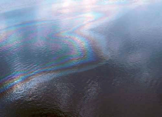
Liquid-phase petroleum released at the ocean surface or sub-sea, once it reaches the ocean surface, will spread on water to form a sheen or slick. The reason a slick appears “slick” is due to the dampening effect on capillary waves by the oil on the surface. The visual appearance of such oil can
be used as an indicator of oil properties as well as state and thickness of the oil slick (Fingas, 2021; see Box 5.2). Most crude and fuel oils are dark brown or black. Diesel fuel is sold in three varieties as clear and dyed red or blue, the color indicating different usages subject to different taxes.
When spread on the water surface to form a slick or changed by mixing with water (e.g., emulsions) oils take on other appearances depending on their interaction with light, viewing angle, atmospheric conditions, wind effects, solar illumination, and water conditions. This affects the detection of spill extent and monitoring during response and remediation efforts (see Chapter 4).
Thin sheens have a very small amount of oil. For thicker oil layers, it is difficult to estimate the thickness of the oil layers exactly (see Figure 5.3). Slick thicknesses also vary over several orders of magnitude, from thin sheens of a few
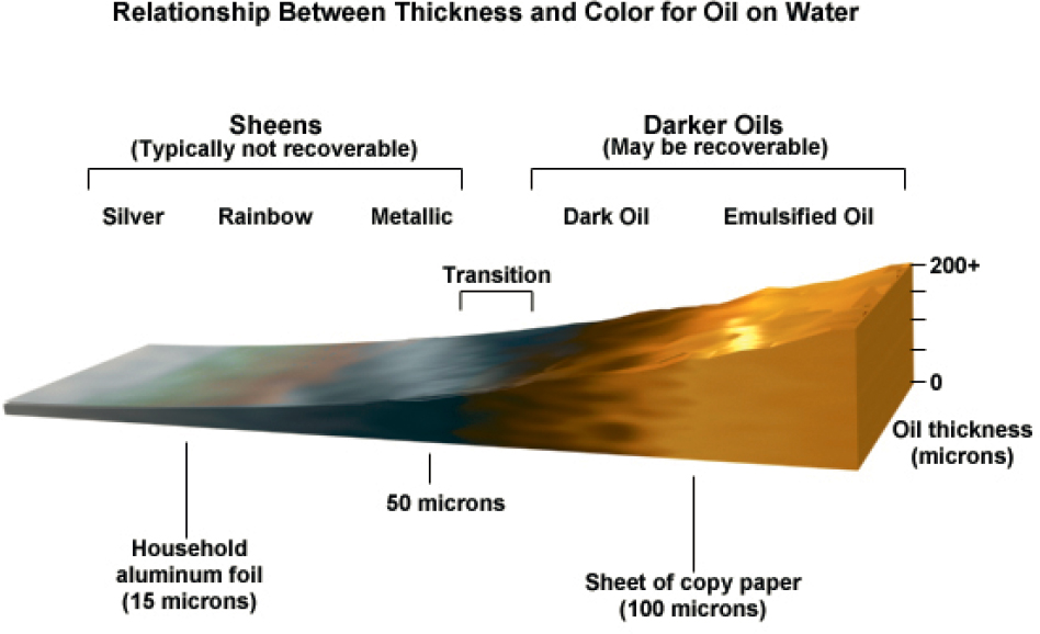
SOURCE: Comet Program, 2014.
micrometers to dark and emulsified oil that may be hundreds to thousands of micrometers in thickness—though still thin, as 1,000 micrometers is only one millimeter thick.
Different color codes have been developed for responders to estimate the thickness of oil slicks. The color codes are generally consistent for thin slicks (<3 µm) but not for thicker portions (>3 µm) that comprise a greater oil volume. For thin oil slicks (thinner than a rainbow sheen; <3 µm), the appearance of oil depends on the thickness of the slick as the optical phenomena involved in oil coloration can be applied. Hence, the appearance of thin slicks is relatively consistent. However, for thicker oil slicks (>3 µm), the appearance of the oil slick is not correlated with thickness because different physical factors predominate and affect the appearance of the slick (e.g., absorption and attenuation of light).
The Bonn Agreement Oil Appearance Code provides a standard method to assess the volume of oil on water based on appearance (Bonn Agreement, 2012). The code classifies the oil thickness into several classes as: sheens (silver/gray), rainbow, metallic, discontinuous true oil color, and continuous true oil color (see Figure 5.4).
Other information that can be obtained from the appearance of an oil slick include coverage and distribution on the surface, formation of water-in-oil emulsions (Lu et al., 2020), indication of oil-in-water emulsions (IPIECA, 2015), rate of emulsion formation (Sicot et al., 2015), measurement of subsea discharge rates (Fingas et al., 1999), and measurement of the oil geometry on the sea (De Padova et al., 2017).
Color also indicates changes due to weathering and response applications. When water-in-oil emulsions form, they often appear reddish in color, depending on the properties of the oil (see Figure 5.6). If dispersant is used as a response method (see Chapter 4), formation of a coffee-colored plume in the water column is a sign of dispersant effectiveness (Cedre, 2005; IPIECA, 2015) and depends on disappearance of oil on the water surface to block the transmission of light into and out of the water column. The brown color develops after the application of dispersants, then slowly dissipates—it is the result of the light reflection from the 5–50 µm droplets dispersed in the water column (Fingas, 2011a). The dispersed plume in the water column may transport in a different direction than the surface slick due to different transport mechanisms (e.g., no wind effect).
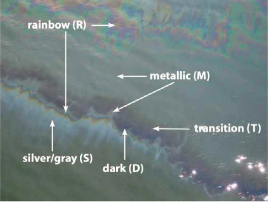
NOTES: Silver sheen (S) is typically <1 µm thick; Rainbow (R) is 1–3 µm thick (see also Figure 5.5); Metallic (M) 3–10 µm thick; slicks of greater thickness and emulsions have inconsistent colors (Fingas, 2021).
SOURCE: From the Open Water Oil Identification Job Aid. Image credit: NOAA.
5.2.2.2 Gas Bubble Breakup
Gas released subsea will form bubbles, and bubbles breaching the sea surface will rapidly enter the atmosphere. Hence, gas-phase petroleum does not form slicks, and the sizes of individual bubbles determine their fate in the water column.
Breakup of gas bubbles is fundamentally different from that of oil droplets due to the low dynamic viscosity and low density of gas compared to oil. As early as Hinze (1955), it was known that it is difficult to disperse gases in liquids due to the high contrast in dynamic viscosities between liquids and gases. This remains true for petroleum gases in seawater, which have a dynamic viscosity ratio of seawater to gas of order 100, indicating that significant energy is required to form smaller bubbles. For most gas releases, the energy available to create a dispersion of bubbles comes from the release rather than ambient ocean currents. For low gas flow rates, bubbles pinch off as their buoyancy lifts them from the release. Even for a very high gas flow rate, the energy input is small due to the low density of gas, which yields a low momentum flux. Wang et al. (2018) observed these facts
SOURCE: NOAA.
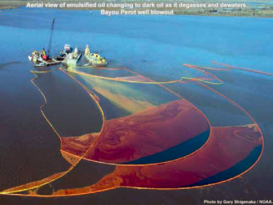
SOURCE: Gary Shigenaka/NOAA.
from experiments on gas jets into a large laboratory tank. Gas jets with large volume fluxes formed large bubbles near the release because the momentum of the gas was insufficient to penetrate very far into the receiving water and form a dispersion. Instead, breakup occurred near a packet of gas surrounding the release. Hence, breakup of gas bubbles is limited in the aquatic environment, and the maximum stable sizes of gas bubbles can be quite large (Clift et al., 1978; Grace et al., 1978).
The dynamics of gas breakup change when a liquid phase is discharged with the gas. This may be a petroleum liquid phase or co-released water. In this case, the higher density of the liquid phase in the release provides significant momentum, allowing the mixture of gas and liquid to penetrate the receiving seawater, generating stronger turbulence and mixing, and leading to greater breakup of gas bubbles. Measurements of bubble sizes for air jets co-released with water are available in Lima-Neto et al. (2008). Data for pure gas jets and a theoretical approach to predict gas bubbles sizes in both types of release are presented in Wang et al. (2018). Wang et al. (2016, 2020) also measured gas bubble sizes distributions for several natural seeps in the Gulf of Mexico. All these studies, which span small to large gas fluxes with and without co-flowing liquids, observe gas bubble sizes in the 2 mm to 5 mm diameter size range, with maximum sizes on the order of 10 mm.
Recent work has adapted theoretical models to predict gas bubble sizes in pure gas releases and for gas released with co-flowing liquid. Zhao et al. (2016) applied a model for gas bubble and oil droplet breakup in a jet that includes the momentum flux of the gas and co-released fluids. Importantly, Zhao et al. (2016) also include the energy input of the bubbles due to their buoyant motion as a contribution to the overall turbulent kinetic energy of the jet. This effect of turbulence production by gas bubbles has been observed in several previous studies. Recently, Lai and Socolofsky (2019) quantify a comprehensive turbulent energy budget for a bubble plume, also showing a significant contribution from the energy input of individual bubbles. Hence, turbulence modulation by bubbles at the bubble scale is an important factor contributing to bubble breakup in large gas-flux releases, such as from accidental marine oil well blowouts. Overall, because of the low viscosity and density of gas, bubble sizes for a wide range of release scenarios fall in a similar, millimeter-scale range and are influenced by the dynamics caused by any co-released fluids.
5.2.2.3 Oil Droplet Breakup and Dispersion
Liquid-phase petroleum, while it is suspended subsea, will form droplets of various sizes. Droplets may form at a subsea release point in a process normally called breakup or as surface floating oil is entrained into the water column through a process normally referred to as dispersion. In either case, turbulent motion in the seawater is responsible for the droplet formation.
Droplet formation of oil dispersed in seawater primarily occurs due to pressure fluctuations at the droplet scale resulting from turbulent eddies in the flow field (Hinze, 1955). To understand how this small-scale turbulent motion relates to the larger turbulent flow, we introduce a few key concepts of the canonical model of turbulence (Pope and Pope, 2000). Turbulent kinetic energy is produced at large scales of the flow, and this energy is transferred to smaller and smaller eddies until reaching the dissipation range, where the length scales are small enough that viscosity (i.e., fluid friction) damps the turbulent energy and converts it to heat. The largest scales of turbulence are highly situationally dependent, controlled by the geometry of the boundaries and the energy input (Tennekes and Lumley, 1972). In the statistically stationary case of steady forcing, the total rate of production of turbulent kinetic energy at the large scales is balanced by the rate of dissipation of turbulent kinetic energy at the smallest scales. Within scales smaller than the production scale but larger than the dissipation scale, Kolmogorov hypothesized that the characteristic length and time scales of the turbulence would depend only on the kinematic viscosity of the fluid and the dissipation rate of the turbulent kinetic energy; this region of the turbulence spectrum is called the inertial subrange, and the turbulent eddies within this region may be considered three-dimensional and isotropic (Pope and Pope, 2000). Because the largest stable droplet sizes of oil are usually small compared to the scales of turbulence production, they may be expected to fall in the inertial subrange of typical environmental flows, where the kinematic viscosity and turbulent dissipation rate fully describe the turbulence. In this way, droplet breakup may be described in terms of these parameters, independent of the larger flow dynamics. However, because the dissipation is intimately linked to the
large scales through the production term, the actual rate of turbulent kinetic energy dissipation, and hence the droplet breakup process, remains specific to each flow situation.
Oil dispersed in a turbulent flow continues to break up until forces within a given oil droplet are large enough to resist further breakup by the turbulent pressure fluctuations. The two properties of oil that resist breakup are the interfacial tension and viscosity. Interfacial tension is the force per unit length along the oil–water interface. As droplets get smaller, the turbulent pressure fluctuations affecting the droplet also become smaller and may eventually become comparable to the interfacial tension forces. When the interfacial tension is very low, however, the viscosity, a form of fluid friction, may also act to limit breakup. Hence, droplet breakup for oil in the sea normally depends on the viscosity and turbulent dissipation rate of the seawater and on the interfacial tension and viscosity of the oil.
There are two basic approaches to predicting droplet breakup within turbulent flows. In the empirical approach, the characteristic scales of the turbulence dynamics and droplet properties are combined through dimensional analysis to yield predictive equations. Box 5.3 applies this approach to define the Weber and viscosity numbers, two key parameters for droplet breakup. Equations to predict characteristic droplet sizes using these parameters must be fitted to experimental data, and are expected to have different fit coefficients in
each type of turbulent flow field. Moreover, these models must assume a probability distribution and width parameter to predict the whole size distribution (see Appendix F). An alternative approach to droplet size modeling involves simulation of the droplet-scale physics of particle breakup and turbulent eddies to predict the time evolution of the whole population of droplets sizes in the droplet size distribution (Zhao et al., 2014a; Nissanka and Yapa, 2016). Key concepts of these population dynamics models are also highlighted in Box 5.3.
The population balance models differ from the empirical equations approach in three main ways. First, because they track the interactions of a full spectrum of droplet sizes, population balance models predict the size distribution directly, without having to assume a probability density function. Second, they consider the time-evolution of the fluid-particle breakup and interaction with turbulence. Hence, they may be applied in cases where the turbulent field is evolving in time, and they can predict the time-dependence of the size distribution in steady and unsteady turbulence. Third, the model equations are based on physics relations at the particle scale. When these scales can be related to the larger-scale turbulent flow, the models can be adapted to a wide range of breakup scenarios, as for example mixing tanks with constant turbulence (Zhao et al., 2014), intermittent turbulence of breaking waves (Cui et al., 2020c), and steady, non-uniform turbulence of blowout jets (Zhao et al., 2014b, 2015, 2016, 2017; Nissanka and Yapa, 2016; Aiyer and Meneveau, 2020). Empirical equations can also be adapted to these flow cases (e.g., Wang and Calabrese, 1986; Johansen et al., 2013, 2015), and in both of these modeling approaches, experimental data are required to calibrate and validate the model predictions.
While bubble and droplet breakup has been a topic of chemical engineering for years, the past 10 years have seen a tremendous increase in models adapted to oil spill scenarios and in laboratory data relevant to oil spills which can be used to calibrate and validate such models. Specific oil spill models and experimental observations in the context of different spill types are reviewed in Sections 5.3 and 5.4. Additional details about the theoretical foundations of empirical equations and models for droplet breakup in turbulent flows are given in Appendix F.
5.2.2.4 Effects of Chemical Dispersants on Droplet Breakup
A recent National Academies committee has comprehensively reviewed the usage of chemical dispersants as response agents for marine oil spills (NASEM, 2020). Here, we briefly explain what dispersants are and how they affect droplet breakup (see also the discussion of dispersants in Sections 4.2.3, 5.3.1.3, and 5.3.3.5).
Chemical dispersants are mixtures of surfactants that are dissolved in one or more solvents. Surfactants have active groups with affinity for oil (i.e., oleophilic or hydrophobic) and affinity for water (i.e., hydrophilic). The orientation of the surfactant at the oil–water interface reduces the interfacial free energy, reducing the interfacial tension. This reduction in the interfacial tension has two main effects on droplet breakup. First, by reducing the interfacial tension, the droplet resistance to breakup is reduced, and smaller droplets will form under the same turbulent conditions as compared to untreated droplets, that is, those naturally dispersed. This effect holds in the primary break-up phase of dispersion in which droplets are formed by interactions with turbulent eddies down to the inertial scale of the turbulence. Second, fluid motion at the oil droplet-water interface can further concentrate dispersant at convergence points at the lee of a rising droplet, leading to singularities in the interfacial tension, that is, zero interfacial tension, at the wake separation points (Gopalan and Katz, 2009, 2010). Oil may then leak through these separation points, forming very thin oil threads, with diameters on the order of a few microns. This effect is a new phenomenon identified since the previous Oil in the Sea report (NRC, 2003) and is known as tip streaming (see Sections 5.3.1.3 and 5.3.3.5). Tip streaming has been observed for oil droplets suspended in homogeneous, isotropic turbulence (Gopalan and Katz, 2010), for droplets rising to the sea surface after passage of a breaking wave (Li et al., 2017), and for droplets stabilized in a counter-flowing water tunnel (Davies et al., 2019). The oil threads leaking from these chemically treated droplets eventually break up by sinuous-wave instabilities along the oil thread, forming droplets with diameters of order 1 micron down to potentially 100 nanometers (Li et al., 2017).
As explained in Chapter 4, dispersants are used to promote smaller droplet sizes because smaller droplets help increase biodegradation rates in the water column and reduce the amount of oil on the water surface, thus reducing the amount of oil that can reach the shoreline. Dispersants may be applied at the sea surface to promote breakup of floating oil slicks into dispersions of suspended droplets (see Section 5.3.1.3). Or, they may be applied locally at the spill source to promote formation of smaller droplets in the primary breakup zone of a release (see Section 5.3.3.5). We discuss the dynamics associated with each of these use scenarios in the cited sections.
5.2.3 Transport and Dilution of Oil and Gas in the Sea
Hydrocarbons released into the sea occur as two different types of tracers: dissolved hydrocarbons are passive, being transported and mixed much like dissolved oxygen; gas bubbles and oil droplets are active, being affected both by the local ocean currents and their own buoyancy and immiscibility. The processes by which passive and active tracers are transported and mixed by ocean processes is the topic of environmental fluid dynamics. A classic treatment of the subject is presented in Fischer et al. (1979); a modern, comprehensive exposition is presented in Fernando (2013a,b).
Transport is a technical term referring to the movement of a dissolved or suspended material with the local currents. Mixing results when a parcel of water is homogenized with another parcel of water. Mixing normally reduces the concentrations of tracers in the combined parcel and reduces the differences between the maximum and minimum concentrations across a tracer cloud. Hence, mixing normally results in dilution of concentrations and homogenization of the concentration field (Fischer et al., 1979). Mixing mechanisms in the ocean include molecular diffusion, turbulent motion, and fluid motion resulting from unstable density fields, among other apparently random processes.
For hydrocarbon transport and mixing in the oceans, all mechanisms and scales of dynamics are present. At the droplet–water and bubble–water interface, molecular diffusion limits transfer of liquid and gaseous hydrocarbons to the aqueous phase (see Section 5.2.6). Outside the bubble or droplet, a chemical boundary layer forms, which is affected by the fine–scale turbulence surrounding the bubble or droplet and its wake. Once outside the concentration boundary layer, dissolved hydrocarbon is affected by ocean currents (advection) and turbulence. Advection is a deterministic transport process that moves dissolved constituents with the local fluid flow. Turbulence causes a random kind of advection that is normally approximated by an enhanced turbulent diffusion process. Diffusion is a random process that moves material from high-concentration regions into low-concentration areas, reducing the concentration of local constituents as they are diffused. Because there are many different scales of turbulent eddies, the turbulent diffusion coefficient summarizing the mixing caused by turbulence scales with the size of the tracer cloud—larger clouds are mixed by larger eddies, giving larger apparent turbulent diffusion coefficients compared to smaller clouds mixed by smaller eddies. Experiments from centimeter- to multiple kilometer-scale are observed to obey the Richardson 4/3-power law, which was summarized for ocean mixing in the Okubo diagram (Okubo, 1972; Fischer et al., 1979). This diagram predicts the apparent turbulent diffusion coefficient as a function of the size of tracer cloud being diffused. Hence, dissolved hydrocarbon diffuses more and more rapidly as the cloud of dissolved material grows in size.
In the oceans, turbulent diffusion normally differs in the horizontal and vertical directions. Because of gradients in the ocean salinity and temperature profiles, the water column is density stratified, with lighter water near the surface and denser water at depth. This density stratification stabilizes the water column and limits mixing in the vertical direction. The total movement of a dissolved compound as a result of diffusion is due to the combined effect of the turbulent diffusion coefficient and the concentration gradient. If the concentration is spatially uniform, diffusion will not be active. In the oceans, concentration gradients are usually smaller in the horizontal direction than the vertical direction, largely due to the density stratification, which promotes lateral motion and inhibits vertical motion. Hence, vertical diffusion, owing to the persistent vertical concentration gradients, is normally the dominant mode of tracer mixing in the oceans.
The net effect of diffusion is to dilute or reduce constituent concentrations. In a turbulent flow, eddies smaller than a tracer cloud erode away at the edges, producing a diffusive effect, but eddies larger than the tracer cloud cause advection, or transport, of the cloud. Eddies by nature are three-dimensional and tend to strain (deform) fluid parcels. Thus, eddies larger than a tracer cloud can tear it into pieces, creating filaments of high concentrations surrounded by dilute or pristine water. This process is called turbulent stirring, and concentrations only reduce after these high concentration filaments diffuse into the surrounding low-concentration waters. Ledwell et al. (2016) report on observations of an inert tracer injected at about 1100 m into the deep Gulf of Mexico near the DWH spill site. They found enhanced mixing near the continental slope and that mixing occurring near the slope resulted in intrusion of mixed fluid into the interior of the Gulf of Mexico. The tracer was clearly identifiable over 12 months after injection, but peak concentrations had reduced by 108 times after 12 months compared to the initial release. These very large dilutions were attributed to stirring of the tracer by boundary currents, mesoscale eddies, and three-dimensional turbulent eddies followed by turbulent diffusion across the high-concentration filaments and ultimately molecular diffusion at the smallest scales of tracer gradients. These observations were for a quasi-instantaneous release, however similar mixing occurs across wider scales for more episodic or continuous injections, such as the DWH oil spill. Hence, ocean currents are effective at reducing concentrations by diffusion, and the resulting concentration cloud is not a homogeneous concentration field but rather a complex, stirred tracer field that may be distributed over large areas.
Many discussions of ocean mixing use the term dispersion to account for mixing by turbulent motions. Dispersion, initially identified by Taylor, refers to the combined effects of diffusion and velocity shear, much like the preceding example on turbulent stirring. Velocity shear stretches concentration patches into elongated forms and sets up concentration gradients between the filaments and surrounding water. Diffusion, whether molecular or turbulent, mixes the sheared concentration patch into the surrounding water. The net effect of dispersion is to spread tracer over a much larger area than diffusion alone, since shear advection is working to stretch concentration patches. It is important to keep in mind that dispersion, though, is the combination of two processes, an advection or transport step caused by a sheared velocity field followed by a diffusion step across the sheared concentration gradient. Here, we reserve the word dispersion to refer to suspensions of gas bubbles and oil droplets in seawater (see Box 5.4) and avoid its use in reference to ocean mixing, using instead turbulent stirring and diffusion.
Gas bubbles and oil droplets can also be mixed by ocean currents, much like tracer clouds of dissolved material. The major difference is their active nature: gas bubbles and oil
droplets normally rise through the ocean water column and remain immiscibly dispersed as bubbles or droplets. As a result, gas bubbles and oil droplets may not remain spread out or diluted after a mixing event. For example, gas bubbles rising out of a subsea layer may form into a plume, converging together into a narrow column of rising bubbles. Also, oil droplets that reach the sea surface will accumulate there, not passing entirely into the atmosphere nor resuspending immediately into the ocean water column. Hence, oil and gas may merge back into high concentration layers after they are initially mixed. This is not possible for passive tracers acted on by diffusion since diffusion is an irreversible process. Thus, the active nature of buoyant oil and gas, as well as ocean particles, is important to keep in mind when considering their mixing. Oil that accumulates on the ocean surface (see Section 5.2.2) often remains floating or suspended near the sea surface, and it is transported and mixed by near-surface currents. Surface transport processes as they apply to floating oil have recently received significant attention, especially through several new field experiments involving large numbers of floating drifters (D’Asaro et al., 2020). Floating material tends to accumulate along lines where two water masses meet and downwelling occurs (D’Asaro et al., 2018; Özgökmen, 2018). These convergence zones can spread oil over long distances but also keep it concentrated along the convergence lines. These submesoscale fronts are important at large scales, but Langmuir currents also predominate at small scales. The distribution of oil throughout the water column in the presence of Langmuir cells is strongly dependent on the droplet sizes of dispersed oil (D’Asaro et al., 2020). In fact, fluctuations in ocean flows below the scales of 10 km are the dominant mechanisms for the initial spread of floating tracer clouds, and neither operational circulation models nor satellite altimeters capture the scales of these flows (Poje et al., 2014). Thus, the complex convergent and divergent field of the ocean surface is critical to understanding the spread of floating oil.
In the remainder of this chapter, we will consider all of the processes discussed here to be summarized by the terms transport and mixing, where transport refers to advection with the currents and mixing to any process that changes concentrations by interactions with local ambient water. Because transport determines the affected environment and mixing alters the concentrations, these mechanisms are critical to an understanding of the fates and effects of oil and gas in the seas. A more exhaustive treatment of mixing and transport are presented in the cited reference monographs (Fischer et al., 1979; Fernando, 2013a,b).
5.2.4 Routes to and from the Atmosphere: Evaporation, Aerosolization, and Atmospheric Re-deposition
The sources of oil in the sea are varied, and their route to the atmosphere is dependent on chemical and physical properties of the compounds found in oil. Gas phase compounds readily enter the atmosphere. The ability of the oil to partition to the gas-phase (evaporate), react with existing atmospheric compounds (oxidize), and form condensed phase airborne particles (aerosolize, also referred to as atmospheric aerosol) is complex. The following sections review what is currently known about the generation and potential deposition of atmospheric gas-phase and aerosol pollutants to and from marine oil sources.
5.2.4.1 Primary Atmospheric Pollutants
Hydrocarbons are a primary gas-phase pollutant. Atmospheric hydrocarbons are mainly derived from evaporated oil and contribute the greatest atmospheric mass of oil pollutants (Middlebrook et al., 2012; French-McCay et al., 2021). If the amount of oil at the sea surface is known, one can estimate the evaporation of hydrocarbons by knowing the volatility of compounds in oil and the environmental conditions (e.g., temperature, pressure, volume). Specifically, there are models available to calculate the mass of gas-phase material from condensed phase compounds. Here we briefly describe available models, key assumptions, and additional considerations to estimate the rate of evaporation of oil in the sea.
The evaporation of specific condensed phase components (e.g., liquid or solid) is fundamentally a function of vapor pressure and mass transfer coefficients, both of which depend on temperature, pressure, and volume. Thus, the amount and rate of evaporated oil can be derived by coupling thermodynamic equations of state, vapor–liquid equilibrium models, and mass transfer equations. Evaporation has been long known to change oil composition on water surfaces; evaporation removes lower boiling point and lower molecular weight components from the liquid phase into the gas phase. The most volatile compounds evaporate in as quickly as an hour (McAuliffe, 1989). Experimental work since the 1970s has measured rates of evaporation from refined and diesel oils (Blumer et al., 1973; Mackay and Matsugu, 1973; Regnier and Scott, 1975) and provided some of the earliest data regarding the evaporation of oil components. The most widely used model to describe the evaporation of oil hydrocarbons and petroleum mixtures is the work of (Stiver and Mackay, 1984). The Jones (1997) model is more advanced and assumes a pseudo-component evaporation model. The Jones model employs components representative of benzene, toluene, ethylbenzene and xylene (BTEX), polycyclic aromatic hydrocarbon (PAH) fractions, volatile aliphatics and two semi-volatile aliphatic fractions. Each component evaporates according to its binned vapor pressure, diffusivity and molecular weight. To date, state-of-the art evaporation models applied to oil spills have been validated and extended the number of components used in Jones to better represent the complexity of oil compositions (Lehr et al., 2002; McCay and Rowe, 2004; Spaulding, 2017; French-McCay et al., 2018). However Jones and subsequent evaporation models rely on parameterizations of a mass transfer coefficient and
simplifications of fuel formulations. Thus, it should be noted that simplified empirical evaporative models, such as the Fingas model have also been applied to oil in marine environments. The Fingas model (Fingas, 1999) is specific for oil types and depends on temperature and time. Regardless of the model, as fuel formulations advance, the evaporative models must keep up to date with changes in new formulations. Additional details of evaporative models for oil in the sea can be found in the recent review by Keramea et al. (2021).
Gas-phase oxidized sulfur (SOx) and organosulfur compounds are emitted into the air from the combustion of sulfur-containing fossil fuels. The higher the sulfur fuel content the larger the potential airborne emissions of combusted SOx. Much research has considered the fates of atmospheric sulfur emissions from varied shipping fuel formulations (Streets et al., 2000; Corbett, 2003; Endresen, 2003; Perraud et al., 2015; Abdul Jameel et al., 2017; Peng et al., 2020; Pei et al., 2021). One of the largest uncertainties from atmospheric SOx emissions has been attributed to the international shipping operations in marine environments (Smith et al., 2011). The International Maritime Organization regulations have gradually reduced the allowable sulfur content of ships’ fuel oil. From 1 January 2020 the global upper limit was reduced from 3.50% to 0.50% mass. Higher sulfur content is allowed if a vessel operates an exhaust gas cleaning system that results in SOx emissions equivalent to burning 0.5% sulfur content fuel. A stricter sulfur limit of 0.10% mass has been applied in Emission Control Areas (ECAs) since 2015. The North American coastal waters were designated as an ECA in 2010, and the waters around Puerto Rico and the U.S. Virgin Islands were designated as an ECA in July 2011; ECA and a timeline of sulfur content requirements are shown in Figure 5.7.
ISO-8217 is a specification of marine fuels by the International Organization for Standardization (ISO). The standard applies to High Sulfur Fuel Oil (HSFO) as well as 0.5% sulfur fuels, generally referred to as Very Low Sulfur Fuel Oil (VLSFO). It is currently under review to update it to reflect the quality changes resulting from the introduction of VLSFOs, recognizing that there are wide variations depending on how the fuel is produced or blended.
It is also noted that fuel sulfur content is positively and linearly related to primary particulate matter emissions (Streets et al., 2000; Corbett, 2003; Endresen, 2003; Perraud et al., 2015; Abdul Jameel et al., 2017; Kim and Seo, 2019; Peng et al., 2020; Pei et al., 2021); high sulfur content fuels contribute to higher particulate matter (PM) concentrations. Thus, several countries have reduced the sulfur content of shipping diesel fuels to ultra low levels of 10–15 ppm (ultra low sulfur diesel) to reduce ship atmospheric emissions that
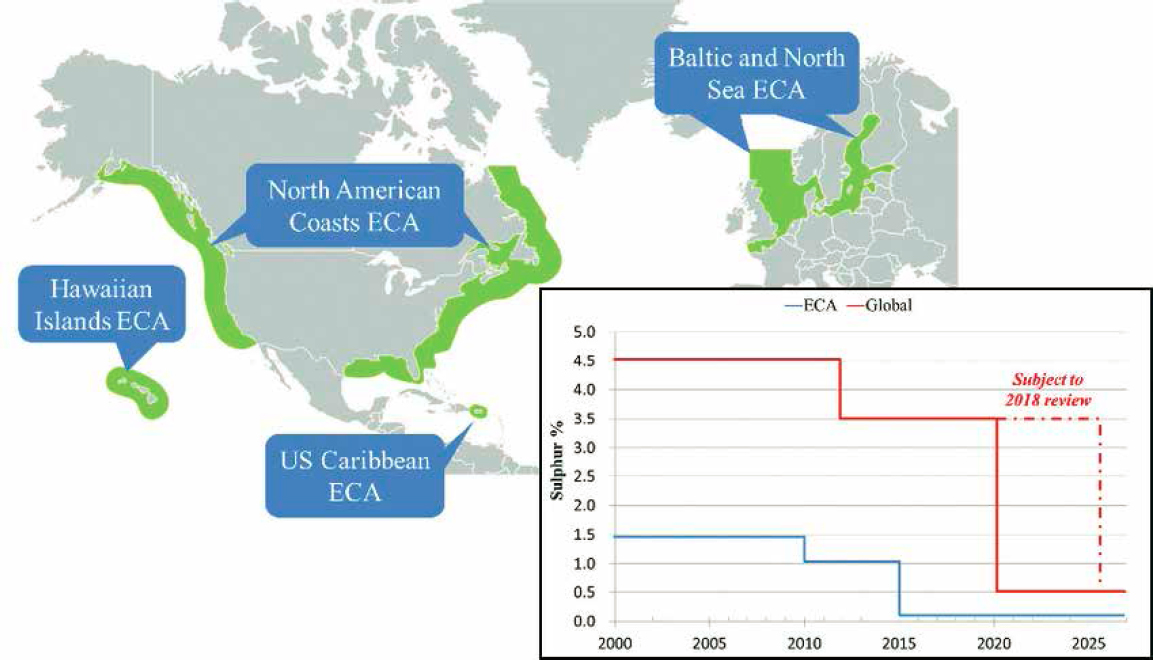
NOTE: The red line indicates global requirements, and the blue line indicates ECA requirements.
SOURCES: Gu et al. (2016); http://dx.doi.org/10.2139/ssrn.2870407.
significantly affect local port communities (Eyring et al., 2005). Furthermore, the use of sulfur-containing biodiesel fuels in marine transportation is of growing interest (Lin, 2013; Price et al., 2017; Mohd Noor et al., 2018; Svanberg et al., 2018; Zhou et al., 2020; Deng et al., 2021).
Indeed, the emissions of oil in the sea may be directly expelled as solid or liquid condensed-phase material (particulate matter or PM). High winds, wave crests, bubble bursting on marine surfaces, and raindrops can generate particles in scales from nanometers to hundreds of micrometers (Blanchard and Woodcock, 1957; Monahan et al., 1983; O’Dowd and de Leeuw, 2007; Ryerson et al., 2011; Murphy et al., 2015). For example, the bubble bursting of surface oil has been shown to directly emit oil droplets into the atmosphere (Ehrenhauser et al., 2014; Sampath et al., 2019) and the use of dispersants can modify the amount of primary gas and aerosol phase material emitted into the atmosphere (Afshar-Mohajer et al., 2018).
Oil that undergoes combustion can also directly emit black carbon or soot-like aerosol into the atmosphere. For example, during the DWH oil spill, black carbonaceous aerosol was measured directly downwind of the source (Perring et al., 2011). Furthermore, extensive literature has measured soot aerosol in marine environments directly attributed to anthropogenic shipping and oil operations (Agrawal et al., 2008, 2010; Moldanová et al., 2009, 2013; Popovicheva et al., 2009; Ault et al., 2010; Zheng et al., 2010; Khan et al., 2012; Lack and Corbett, 2012; Browse et al., 2013; Gaston et al., 2013; Tao et al., 2013; Buffaloe et al., 2014; Cappa et al., 2014; Celo et al., 2015; Kleinman et al., 2016; Betha et al., 2017; Streibel et al., 2017; Corbin et al., 2018; Fingas and Lambert, 2018; Jiang et al., 2018; Zhang et al., 2019). Many of the aforementioned studies also quantify the co-emission of regulated pollutants, such as carbon dioxide and nitrogen dioxide that contribute to global warming and the oxidation of secondary pollutants. Indeed, carbon dioxide and its greenhouse gas considerations can be primary and secondary atmospheric pollutants as considered in the following section.
5.2.4.2 Formation of Secondary Pollutants
The chemical reactivity of hydrocarbons can lead to the formation of secondary gas-phase and aerosol pollutants. Natural gas operations are sources of hazardous pollutants and photochemical ozone precursors that can produce secondary ozone (Kemball-Cook et al., n.d.). These aged organic vapors may undergo fragmentation (breaking of carbon–carbon bonds) and functionalization (e.g., the addition of polar functional groups), and the contribution of oxidation products to secondary pollutant concentrations continues to be of scientific interest. Several semi-empirical parameterizations have been applied (Robinson et al., 2007; Hodzic et al., 2010; Shrivastava et al., 2015), but more is needed to address the complex chemistry. Additionally, the chemical reactivity of intermediate volatile organic compounds (VOCs) (C14–C18) can lead to the formation of higher molecular weight products to create secondary organic aerosol, SOA (de Gouw et al., 2011). Aerosol scientists use knowledge of chemical reactions (e.g., photochemistry) and thermodynamic models to estimate the formation of SOA from hydrocarbons. The volatility basis set (Donahue et al., 2006, 2011, 2012), is an empirical model that assumes that volatility of the gas and condensed phases materials is in equilibrium for a concentration range.
It also should be noted that the combustion and oxidation of reactive hydrocarbons ultimately leads to the formation of atmospheric CO2. Thus, for the formation of greenhouse gases (natural and anthropogenic) from oil sources, it should also be considered (McAlexander, 2014) whether they are primary (e.g., methane) or secondary (e.g., CO2, N2O) greenhouse gas atmospheric pollutants.
More research is needed to understand the formation of secondary air pollutants immediately downwind and transported long range from oil in the sea sources.
5.2.4.3 Deposition of Atmospheric Pollutants in the Marine Environment
Currently, the deposition of gas-phase and aerosol pollutants derived from oil sources into the marine environment is not well quantified. In this section, we review key papers that provide information regarding oil sources from the atmosphere and the biogeochemical cycle into the marine environment.
The mass transfer at the air–sea interface is complex. Much of the work addressing this exchange is derived from our understanding of PAHs (see Section 3.3.2). PAHs are ubiquitous in the atmosphere, can be transported over long distances, and are compounds of interest to quantify the biogeochemical cycles from oil in the marine environment. PAHs are natural and anthropogenic in origin; they are mainly derived from the incomplete combustion of fuels. Atmospheric PAHs in the marine environment have been measured in coastal areas and across several oceans; the measured PAH concentration varies in different seas (Ding et al., 2007; Nizzetto et al., 2008; Castro-Jiménez et al., 2012; Wang et al., 2013; Ke et al., 2017; Pegoraro et al., 2020). Recent work has measured and characterized the dry and wet deposition of PAHs into seawater (Castro-Jiménez et al., 2012; Lammel et al., 2016; Everaert et al., 2017; Chen et al., 2021) but more work is required to quantify the contributions of oil derived PAH sources back into the sea. Oceans are considered a major sink for long-range transport air pollutants (e.g., CO2, and PAHs) (Wania and Mackay, 1996; Dachs et al., 2002; Lohmann and Belkin, 2014). Long-range transport air pollutants can be long-lived and therefore specific air pollutant tracers from oil industries must be identified to directly assess the impact of oil in the sea. The identification of such tracers are critical for understanding the air-water exchange, and the overall biogeochemical cycle of pollutants.
5.2.5 Photochemical Reactions
There has been a significant advance over several decades in our understanding of the role of photochemical reactions in the fate of spilled oil, and perhaps by extension to some of the other types of petroleum or oil inputs to the marine environment. Renewed appreciation of photochemical reactions has resulted in a paradigm shift, causing us to consider photochemical reactions as one of the major factors influencing the fate of spilled oil at the sea surface. In addition, there are implications for better understanding the effects of oil photochemical reaction products in concert with other processes influencing the fate of oil inputs as will be discussed below. Furthermore, this new knowledge has important implications for understanding effects of oil on marine organisms to be discussed in Chapter 6 of this report.
Photo-oxidation, sometimes referred to as photochemistry in some papers and reviews, was recognized in oil spill research of the late 1960s and early 1970s as one of the processes contributing to the fate of spilled oil slicks and sheens (NRC, 1975). An influential paper by Burwood and Speers (1974) aptly noted the importance of photo-oxidation as a factor in the dispersal of crude oil slicks. The importance of photo-oxidation was further emphasized in the literature reviewed by Payne and Philips (1985) and the report Oil in the Sea (1985). The process of photo-oxidation is also of concern because of research demonstrating that such reactions can produce products that are toxic (NRC, 1975, 1985, 2003; Lee, 2003, and references therein) as will be discussed in Chapter 6. As noted in the preceding references, initial attention was focused on photo-oxidation of aromatic hydrocarbons and aromatic ring compounds containing nitrogen due to experiments that indicated a few of these types of reactions yielded compounds with toxicity to marine organisms.
Photo-oxidation is often used as the overarching term in oil pollution literature and may appear in the citations and discussion that pertain in this report. However, it is important to recognize that at least three processes are recognized to occur, or have the potential to occur, during photochemical reactions of oil as suggested by Overton et al. (1980) and more recently demonstrated through research during the past 10 years (Rodgers et al., 2021; Freeman and Ward, 2022):
- Direct/indirect photo-oxidation
- Photo-induced polymerization
- Photo-cracking of large molecules
One type of photochemical reaction that might occur is photosensitized oxidation as outlined in simplified form in Figure 5.8. This depicts a compound other than the compound of interest, the simple hydrocarbon n-hexadecane, being activated by light energy to a triplet state and then subsequently a series of resulting follow-on reactions. Figure 5.9 depicts other mechanisms of photo-oxidation of petroleum hydrocarbons including those involving singlet oxygen.
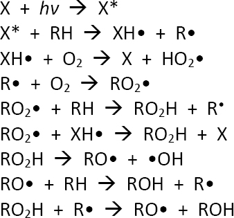
NOTES: X is xanthone; hv is light; X* is the xanthone triplet; RH is n-hexadecane; XH• is the hydrated xanthone radical; R• is the n-hexadecane free radical; O2 is molecular oxygen; HO2• is the hydroperoxy radical; RO2• is the n-hexadecane peroxy radical; RO2H is n-hexadecanoic acid, RO• is the oxygenated n-hexadecane radical; •OH is the hydroxyl radical; ROH is n-hexadecanol. Xanthone is an example of one of several photosensitizers that could be encountered in the environment of an oil spill.
SOURCE: Adapted with permission from Gesser et al. (1977). Copyright 1997, American Chemical Society.
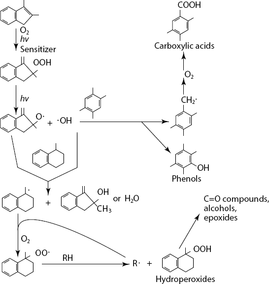
SOURCE: Adapted with permission from Payne and Phillips et al. (1985). Copyright 1985, American Chemical Society.
These are representative reaction diagrams discussed by Payne and Phillips (1985). Given the thousands of hydrocarbons in crude oils, as discussed in Chapter 2, it was not difficult to imagine that there might be many thousands of photo-oxidation reaction products. Applications of advances in analytical chemistry to field samples and samples from laboratory experiments post-DWH spill have shown that there are indeed many thousands of reaction products. This presents new challenges as will be discussed.
Research since the NRC (2003) report explores various aspects of the photochemical reactions involving oil and oil compounds (e.g., Aeppli et al., 2012; Corea et al., 2012; Ray and Tarr, 2014a,b; Cao and Tarr, 2017; Ward et al., 2018b; Wang et al., 2020). A reasonably comprehensive review of research by different groups of investigators, including relevant papers from the 1970s onward, of both laboratory experiments and field observations (mainly from the DWH related research 2010 to 2020) of photo-oxidation as it relates to the fate of spilled oil in the marine environment is presented by Ward and Overton (2020). They build upon the early research summarized in reviews such as that of Payne and Phillips (1985), and NRC (1985). They note that the need to incorporate photo-oxidation as a component of oil spill fate and trajectory modeling was stated by Spaulding (1988).
Inclusion of photochemical reactions in oil spill modeling has begun in part with the paper by Ward et al. (2018b). They combined results from laboratory experiments, field sampling and analysis, field observations, and modeling to demonstrate that for the DWH oil spill photo-oxidation of oil compounds in the surface slick converted many compounds to reaction products and was a significant quantitative fate for these compounds. The reaction products may then undergo further degradation by microbial or other biological processes, although this has yet to be determined. This finding is at odds with the prevailing wisdom or assumptions pre-DWH. It is a significant update to what was stated in Oil in the Sea III (NRC, 2003).
The Oil in the Sea III report contained a statement in the section “Photo-oxidation in Sea Water” in the Behavior and Fate of Oil chapter, pages 94–95: “(Parker et al., 1971, cited in Malins, 1977) Photo-oxidation is unimportant from a mass balance consideration: however, products of photo-oxidation of petroleum slicks may be more toxic than those in the parent material (Lacaze and Villedon de Nevde, 1976).” In hindsight that statement is perplexing. The latter citation does not deal with mass balance consideration. It is focused on photo-oxidation products that cause toxicity. The statement about “from a mass balance consideration” seems to be based on a conceptual model that emphasized other processes such as evaporation, dissolution, and biodegradation.
A similar concept or assumption was incorporated into various field response guidance manuals (NOAA, 2013a; ExxonMobil, 2014; Ward and Overton, 2020). As is often the case in scientific research, new findings require revisions to previous assumptions. Informed by new research, the current understanding, based on recent published research as noted above, is depicted in the paradigm of Figure 5.10 (Ward et al., 2018b). These are generalized representations
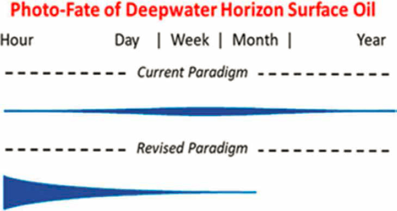
NOTES: Revised paradigm refers to post-DWH research and revisiting photo-oxidation of oil slicks circa 1971 onward (e.g., Ward et al., 2018b; Ward and Overton, 2020). Intensity of photochemical action on the surface oil slick begins earlier and is more intense than previously depicted and comparable to evaporation as a weathering process in published paradigms similar to this figure (see Ward and Overton, 2020). As noted in this report in Chapter 2 and this chapter, each set of chemical constituents in the various types of oil have specific relative fates with their own time-dependence and depending on the geographic/ecosystem location.
SOURCE: Ward et al. (2018b). Copyright 2018, American Chemical Society.
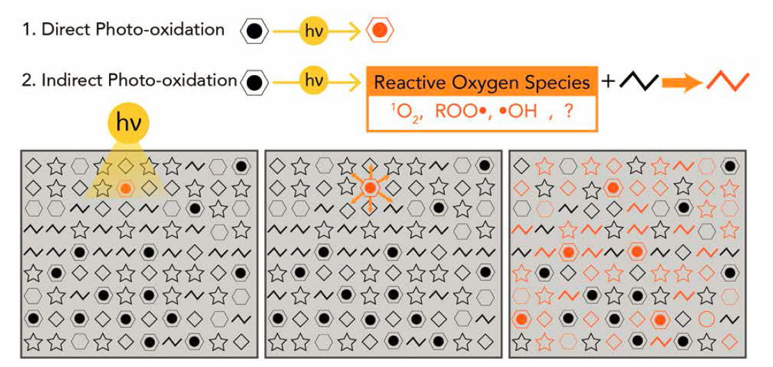
NOTES: In direct photo-oxidation (Reaction 1) a light absorbing molecule (depicted as a black aromatic ring) is partially oxidized into a new molecule (depicted as an orange aromatic ring). Indirect photolysis occurs when the absorption of light (Reaction 2 and left panel) leads to the production of reactive oxygen species (middle panel), like singlet oxygen, peroxyl radicals, and hydroxyl radicals. These reactive intermediates can oxidize a wide range of compounds, not just the compounds that directly absorb light (right panel).
SOURCE: From Ward and Overton (2020) with permission.
(NOAA, 2013a; ExxonMobil, 2014) that must be evaluated in terms of type of oil spilled and the climate regime (e.g., insolation, temperature) and ecosystems involved. Nevertheless, it is clear that photo-oxidation has re-emerged as an important factor in understanding fates of oils spilled in the marine environment.
The evidence for both direct and indirect photo-oxidation of oil components is summarized by Ward and Overton (2020). Their Figure 5 is presented here as Figure 5.11. As noted in the section of this report on advances in analytical chemistry (see Section 2.3), the ability to characterize reaction products by high magnetic field Fourier-transform ion-cyclotron-resonance mass spectrometry (FT-ICR-MS), and other high-resolution mass spectrometric methods, in several ionization modes has enabled new understanding of oil photooxidation reactions and reaction products and their fates (e.g., Niles et al., 2019, 2020). Considering the thousands of petroleum hydrocarbons and other less prominent compound classes containing heteroatoms of oxygen, nitrogen and sulfur (O, N, and S) that can be present in crude oils, fuel oils of various types and lubricating oils, among other fossil fuel oils, both direct and indirect photo-oxidation reactions can yield a myriad of reaction products. Hydrocarbons can yield photooxidation products that contain one to multiple oxygen atoms. In addition, N and S-containing compounds in crude oils yield photo-oxidation products with multiple oxygen atoms.
Zito et al. (2020) report the formation of water-soluble products from photo-oxidation of oil that form interfacial material (IM) at the oil–water interface in laboratory experiments. The photo-oxidation products then progressively become part of the dissolved organic matter (DOM). Figures 5.12 and 5.13 provide a glimpse of the complexity of reaction products produced by photo-oxidation of a Macondo surrogate oil spread on a thin film of pre-irradiated sea water and exposed to simulated sunlight in a laboratory experiment (Zito et al., 2020). The heteroatom class of reaction products and how photo-oxidation reactions produce a sequence of products proceeding over time from oil is depicted in Figure 5.12. Figure 5.13 comes from the same samples and further delves into the heteroatom composition in a van Krevelen plot of O/C versus H/C (O = oxygen, H = hydrogen, C = carbon). Each dot in Figure 5.13 represents a molecular formula. The elemental formulas for the reaction products are known; however, some of the general pathways of photochemical reactions are known (e.g., see Figure 5.11 and also Ray and Tarr, 2014a,b). Except for relatively few specific examples, the details of the exact molecular structures of both the reaction intermediates and reaction products are not known at this time.
By extension from natural organic compounds, a reasonable assumption is that some of the photo-oxidation reaction products are susceptible to microbial degradation. Likewise, uptake and metabolism by at least some multicellular marine organisms is likely. However, this has yet to be explored in any substantive manner. Moreover, the interactivity of the photochemical reaction products
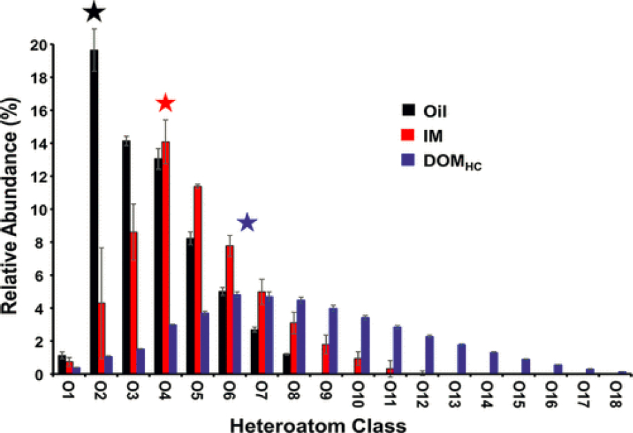
NOTES: Black star indicates the most abundant species in the O2 class in the oil soluble species contain 1–8 oxygens. The interfacially active species contained 1–12 oxygens and had an increased tendency to bind water and remained associated with oil. The most abundant IM components contain four oxygens per molecule (red star). DOMHC are the most water soluble species and had 1–18 oxygens per molecule with the most abundant having 6–7 oxygens per molecule (blue star).
SOURCE: Zito et al. (2020). Copyright 2020, American Chemical Society.
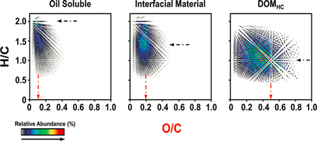
NOTES: Black and red arrows highlight the most abundant H/C and O/C values, respectively. C(carbon), O(oxygen), H(hydrogen).
SOURCE: Zito et al. (2020). Copyright 2020, American Chemical Society.
in sorption/desorption processes with particulate matter from mineral particles to larger marine snow complex assemblages of particles (see Section 5.2.2) is a reasonable hypothesis yet to be tested in a substantive manner.
The photochemical reaction products formed at the sea surface and subsequently part of the oil slick or oil sand mixture coming ashore on beaches results in a conglomerate of resin-like and asphaltene-like material along with photooxidation products that are residual oil soluble and associated with the sediment-oil-agglomerates (SOAs) and oiled sand patties (e.g., John et al., 2016; White et al., 2016; Harriman et al., 2017, 2018; Aepelli et al., 2018; Bostic et al., 2018; Bociu et al., 2019; see Section 5.3.2).
Given that there is evidence that these SOAs can last as long as 32 years (Bociu et al., 2019) it is important to ascertain what specific reaction products are present, their fate, and potential for bioavailability to young children (toddlers) as noted in Chapter 6.
Marshes are another area of shoreline research that has documented the importance of the resin-like and asphaltene-like photochemical reaction products in the persistence of tar mat-like materials for at least several years (e.g., Lin et al., 2016).
In summary, research of the past 10–15 years has documented unequivocally the importance of photochemical reactions in the mass balance loss and fate of spilled oil at the air–sea interface in slicks and in films in temperate and subtropical regions. Variations of intensity of sunlight (various wavelengths) and corresponding variations in photo-oxidation reaction rates can be expected depending on sunlight intensity (insolation and angle of sunlight to the surface), cloud cover, day length and temperature, particularly in the polar regions (e.g., see Freeman and Ward, 2022).
Ward et al. (2018a) present compelling evidence and arguments that new findings of the photochemical chemical reactions of the oil at the sea surface have important implications for response, damage assessment, and restoration activities related to oil spills. For example, many of the photo-oxidation products have various oxygenated functional groups and free radicals that enhance interactivity of water and oil (as noted above), perhaps causing emulsions and/or interfering with and decreasing the efficacy of present-day dispersants, herders, or emulsion treating agents. Moreover, the emergence of the greater importance of the photochemical reaction processes requires more extensive and intensive research focused on interactions of the photochemical reaction products with other aspects of the fates and effects of oil inputs such as slick thickness, emulsification, and biodegradation. This is important for all geographic regions.
5.2.6 Dissolution
Dissolution is the process by which components in a gas- or liquid-phase petroleum fluid are transferred to an aqueous dissolved state in seawater. The solubility is the maximum amount of a given compound that may be dissolved in water at equilibrium with the dissolving mixture; the corresponding component concentration is the saturation concentration. Solubility for pure compounds and petroleum mixtures has been described in detail in Section 2.4. Dissolution occurs as long as the water phase has not reached the solubility limit. Hence, dissolution is inherently an unsteady (time-evolving) process with a rate controlled by the dissolution kinetics. In the oceans, ambient concentrations are low and the saturation concentration is rarely encountered so that dissolution is a continuous process for submerged petroleum fluids.
Directly at the interface between a petroleum fluid and water, dissolution is rapid, and the saturation concentration is expected to occur. As long as the concentration in the bulk water phase far from the interface is below saturation, dissolved components will diffuse away from the interface. This diffusive flux is matched by ongoing dissolution at the petroleum–water interface. Using the analytical solution for diffusion from a constant-concentration interface, one may write the rate of dissolution, or mass transfer dmi/dt, of a component i from the petroleum to the aqueous dissolved state as
| (5.1) |
where A is the area of the interface, Cs,i is the solubility of compound i, Cb,i is the concentration of compound i in the bulk water, and βi is a mass transfer coefficient for component i, also called the mass transfer velocity (Clift et al., 1978).
The mass transfer coefficient encapsulates the thermo- and fluid-dynamic processes occurring in the thin concentration boundary layer near the petroleum–water interface. This includes molecular diffusion of component i away from the interface, convective or turbulent transport of component i through the concentration boundary layer, and the thickness of the concentration boundary layer itself. Because these properties are different at different water temperatures, for different interface types, for example bubbles or sheens, and for different conditions of fluid motion, the value of the mass transfer coefficient depends on the in situ conditions where dissolution is occurring. General behavior of dissolution mass transfer from floating oil and suspended droplets and bubbles is discussed below. More details related to specific spill scenarios are discussed in Sections 5.3 and 5.4.
5.2.6.1 Dissolution Mass Transfer from Floating Oil
Oil floating on the sea surface is exposed to both seawater at its bottom interface and the atmosphere at its top interface. Mass transfer from the floating oil to the atmosphere is by evaporation, or volatilization; this is discussed in Section 5.2.4. At the same time, dissolution may be occurring at the petroleum–water interface of the surface slick and for oil droplets suspended in the water column by natural dispersion. Dissolution from suspended droplets
is considered below. MacKay and Leinonen (1977) suggest using Equation 5.1 for dissolution mass transfer from a surface slick, and they proposed a single value of the mass transfer coefficient for all compounds in the oil of βi = 2.36 × 10⁻⁴ cm/s, which was experimentally derived for experiments on oil slicks in ponds. This approach was also used by McCay (2003) and French-McCay (2004) to assess potential damages of surface spills. For different wind and sea states, the mass transfer coefficients may be quite different (MacKay and Leinonen, 1977); however, because all soluble components in an oil are also volatile, there is a competition between evaporation and dissolution for mass transfer out of the liquid-phase petroleum of the surface slick. Because mass transfer by evaporation in some of the light molecular weight hydrocarbons is up to 10 times that by dissolution, dissolution has been a less important process for mass balance calculations of surface floating oil (MacKay and Leinonen, 1977). Toxicologically, dissolution is always important, and for Arctic oil spills where ice coverage may restrict or eliminate evaporation, dissolution from surface floating oil under ice may be particularly important.
5.2.6.2 Dissolution Mass Transfer from Suspended Gas and Oil
Unlike for floating oil, suspended oil droplets and gas bubbles are not exposed to the atmosphere, and all mass transfer from the petroleum to the aqueous phase must be by dissolution—evaporation, or volatilization, does not occur. As a result, dissolution may be a significant fate process for the mass balance of petroleum fluid spilled subsea. When oil and gas are released subsea, they break up into droplets and bubbles (see Section 5.2.2). Hence, dissolution will occur following Equation 5.1 with mass transfer coefficients applicable to droplets or bubbles. The rate of dissolution changes as the surface area, mass transfer coefficient, and solubility change. These parameters in turn change due to changes in seawater temperature and pressure as bubbles or droplets rise as well as by the evolving composition of the droplet or bubble as they dissolve.
Oil may also be found subsea in the form of various oil-particle aggregates (OPAs; see Box 5.9 later in this chapter). Mass transfer coefficients from solid particles are similar to those for droplets, but in the case of aggregates, not all of the oil will be exposed to water. Because mass transfer rates are not uniform over the surface of a suspended particle, the dissolution rate cannot simply be adjusted by the fraction of exposed oil. Instead, case-specific mass transfer rates would have to be developed for each oil–particle mixture.
Clift et al. (1978) reports on classical understanding of mass transfer from bubbles, drops, and particles. Mass transfer depends on the shape of a fluid particle and whether there is circulation inside the particle. Shapes are classified as spherical, ellipsoidal, or spherical cap, and depend on the fluid particle volume, density, and interfacial tension and on the density and viscosity of the continuous phase seawater (Clift et al., 1978; Zheng and Yapa, 2000). Circulation may occur inside a fluid particle as a result of fluid motion at the particle–water interface. In very clean systems, the interface will move due to the applied drag force from the continuous phase water, setting up a circulation cell within the fluid particle. This circulation enhances convection through the concentration boundary layer, resulting in higher values of the mass transfer coefficient for clean fluid particles. In contaminated systems, Marangoni forces result from concentration gradients of surfactants occurring at the interface of the fluid particle and resist the motion forced by the continuous phase drag. This effect shuts down the circulation within the droplet or bubble, resulting in less convection within the concentration boundary layer. As a result, mass transfer coefficients for contaminated, or dirty, fluid particles are lower than those for clean bubbles or droplets. This effect is expected both for naturally occurring surfactants and for surfactants mixed with the bubbles or droplets by chemical dispersant addition. Clift et al. (1978) provides correlation equations for mass transfer coefficients for fluid particles in a wide range of conditions; Johnson et al. (1969) provides a unified equation for mass transfer coefficients of clean bubbles across the full scope of bubble shapes.
Because of the ubiquitous nature of surfactants in the environment, dirty bubble dynamics are expected in most natural systems; however, several studies in the oceans indicate that clean bubble mass transfer rates may be appropriate early after release of a droplet or bubble. Rehder et al. (2002, 2009) report on measurements of methane bubbles released from a remotely operated vehicle in the deep Monterey Bay, California. They observed bubble size over time, allowing estimation of the shrinkage rate. Shrinkage rates over the first few minutes after release were consistent with mass transfer rates for clean bubbles. During this time, some bubbles shrank by up to half their diameter, which is equivalent to 83% of the volume. Thus, clean bubble mass transfer rates may be important for the initial dissolution of bubbles or droplets released into the oceans.
Likewise, Olsen et al. (2019) released methane gas from diffusers at 100 m and 300 m depth in Trondheimsfjord, Norway. Bubble sizes were initially in the range of 5 mm to 7 mm, in agreement with the observations reported in Section 5.2.2.2. They tracked the bubbles, measuring their diameters until they shrank to 2 mm. Similarly to Rehder et al. (2002, 2009), Olsen et al. (2019) observed that bubble shrinkage rates correlate with clean bubble mass transfer coefficients initially and transition to dirty bubble shrinkage rates at sizes between 3.5 and 4.5 mm. McGinnis et al. (2006) similarly suggested 3.5 mm as the transition size for switching from clean to dirty bubble mass transfer rates using the data in Rehder et al. (2002). In the Olsen et al. (2019) experiments, hydrate formation would not be expected owing to the shallow depths; whereas, for Rehder et al. (2002, 2009), hydrate skins were observed to form on the bubbles
released within the hydrate stability zone. Like the effect of surface contamination, hydrate skins would create a rigid bubble–water interface, similar to the behavior for dirty bubbles. Based on these studies, it appears that clean bubble mass transfer coefficients are appropriate for predicting mass transfer from bubbles in the ocean initially after their release. After some time, mass transfer reduces to dirty bubble mass transfer rates, either due to surfactant contamination (Olsen et al., 2019) or also hydrate armoring (Rehder et al., 2009; Wang et al., 2020).
Although the 3.5 mm transition scale used by McGinnis et al. (2006) agreed with the experiments presented by Rehder et al. (2002), some of the results of Rehder et al. (2009) show different transition points. Wang et al. (2020) considered the Rehder et al. (2009) data and postulated that the hydrate growth rate should depend on the hydrate subcooling and that the time for hydrate growth to complete should be proportional to the initial bubble surface area. Using these parameters, they fitted an empirical model that could predict the transition time from clean- to dirty-bubble mass transfer rates as observed in the Rehder et al. (2002, 2009) datasets. They validated this model to observations of rise height for natural seeps in the deep Gulf of Mexico. We discuss this aspect of their work in Sections 5.3.3.4 and 5.4.1. This approach is also consistent with Vasconcelos et al. (2002), who correlated contamination time with bubble surface area. Despite some uncertainty in contamination mechanisms and transition times, mass transfer coefficients for clean and dirty bubbles have been well studied in the literature, and reliable correlations (e.g., Clift et al., 1978) for each bubble type are well known and tested. Significant new data exist for bubble dissolution rates in the oceans. These data show initial clean-bubble mass transfer behavior followed within minutes or seconds by dirty bubble mass transfer rates. There remains a research need to understand the mechanisms modulating bubble mass transfer rates in the oceans and to collect new observations of mass transfer of bubbles co-released with oil, which may act as a surfactant and inhibit any clean-bubble mass transfer observed in pure-gas plumes.
5.2.7 Emulsification
Oil–water emulsions at sea form by wave action and affect the weathering processes and cleanup options after oil spills. Emulsions consist of a mixture of small droplets of one liquid that remain dispersed in another liquid; see Box 5.4 for definitions. When oil and water are mixed, for example by wind and/or wave energy, two types of emulsions may form depending on the relative quantity of one liquid in the other: water-in-oil emulsions and oil-in-water emulsions (see Figure 5.15). Water-in-oil emulsions, which are also referred as “chocolate mousse” due to their appearance, have water droplets dispersed throughout the oil (Zafirakou, 2019). Water-in-oil emulsions can contain as much as 80% water and can remain floating or submerge (Overstreet and Galt, 1995). Different oils have different susceptibility to emulsion formation and different stability of emulsions that do form, some persisting for a few hours or days and other remaining emulsified for decades. Oil in this form is difficult to degrade because of its high viscosity and reduced surface area. In addition, emulsified oil exhibits reduced evaporation, dissolution, entrainment into the water column and transport (reviewed by French-McCay et al., 2021).
Oil-in-water emulsions, on the other hand, have oil droplets dispersed throughout the water column by the action of agitation, such as wind and wave activity. Dispersing floating oil as droplets (i.e., forming oil-in-water emulsion) increases the oil–water interface and therefore, enhances dissolution of water-soluble fractions and availability of hydrocarbons for biodegradation. These types of emulsions are considered in more detail in Section 5.3.1.3 (natural dispersion).
Droplet sizes of oil-in-water emulsions are related to viscosity and turbulence levels at sea. Lower viscosity and higher turbulence increase formation of droplets and exposure of oil to water column, while entraining smaller droplets. The droplet diameter in emulsions can be estimated from the Weber and Reynolds numbers (Boxall et al., 2012). Stable emulsions have droplet diameters of 8 microns or less and they start to become unstable at droplet sizes of about 50 microns (Opedal et al., 2009).
The interface between the incorporated water and the oil needs to be stabilized in order to form an emulsion (Fingas and Fieldhouse, 2014, 2015). For oil-in-water emulsification, resins facilitate emulsion formation, and they also act as solvents for asphaltenes that support emulsion stability. Although earlier studies reported that as an emulsion forms, water content increases exponentially (MacKay and Zagorski, 1982), later studies showed that characteristics and composition of oil are important for formation of stable emulsions. An emulsification stability index (SI) was developed by Fingas and Fieldhouse (Fingas and Fieldhouse, 2009, 2011; Fingas, 2011a,b) based on stabilizing oil components of asphaltenes and resins, combined with general oil properties of density and viscosity. The emulsification SI can be used to determine whether an oil is unstable, entrained water-in-oil state, meso stable, or stable. Certain microbial species, including those that degrade hydrocarbons, can enhance emulsification and stabilize emulsions through production of extracellular biosurfactants such as rhamnolipids and glycolipids (Gutierrez et al., 2013; Das et al., 2014).
Understanding the processes that lead to emulsification allows better predictions as to when emulsification will occur (Bacosa et al., 2015). In this report, the term “emulsion” is used to refer to oil-in-water emulsions. Processes that promote emulsification include changes in oil characteristics caused by evaporation, photo-oxidation, spreading, and dissolution; and increase in oil viscosity. In flume studies with Macondo oil, over the period of a week, the emulsion viscosity increased, becoming stable in the first 3 days, with
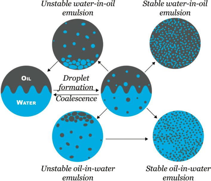
SOURCE: Lee et al., 2015. This content has been reproduced with the permission of the Royal Society of Canada.
the viscosity increasing from 1,000 mPa to over 11,600 mPa over 12 days (Daling et al., 2014). As the emulsification process continues, some emulsified oil sinks; and oil spreading and vertical mixing is reduced (Xie et al., 2007). Recent research in emulsified oil has focused on the effects of photo-oxidation on the initiation of emulsion formation (e.g., Zito et al., 2020), as photo-oxidation of some hydrocarbons makes them more water soluble, thus facilitating formation of an oil–water emulsion. Furthermore, UV irradiation leads to a reduction of micelle size of surfactant molecules beyond that achieved using visible light, and increases the viscosity and stability of the emulsion to freeze–thaw cycles (Genuino et al., 2012).
Daling et al. (2003) provided the findings from four oil release experiments in the North Sea and Norwegian Sea with surface and subsurface oil releases and laboratory studies that involved emulsification. The results of laboratory experiments and full-scale field experiments revealed that both the physico-chemical properties of the oils and the release conditions control the initial film thickness and rate of emulsion formation (Daling et al., 2003). Simulated underwater pipeline release experiments indicated that, within a limited area, the oil droplets surface, forming oil slicks with adequate thickness to support emulsion formation. At moderate depths (300 m), simulated underwater blowout experiments resulted in the gas-bubble plume surfacing, bringing with it entrained water. In deep waters (>500 m), the simulated blowout showed that the plume may be confined to the water column. In this case, the oil droplets will rise to the surface within a more limited area, leading to initial oil film thicknesses that are appropriate for emulsion formation. These studies were used to estimate the timing for dispersant use after the DWH spill (Zito et al., 2020).
Because emulsification has such profound effects on the behavior of oil, French-McCay et al. (2021) persuasively articulate that additional research is needed to improve prediction of oil emulsification, including formation, stability, and behavior, beyond the existing model algorithms.
5.2.8 Microbial Biodegradation of Oil
5.2.8.1 Microbes in the Sea: Who Is Out There and How We Know
Marine systems harbor diverse microbes in astonishing abundance: the world’s oceans have been estimated to contain 1029 microbial cells (Whitman et al., 1998), perhaps exceeding the number of stars in the universe 100,000-fold. A single milliliter of seawater may harbor more than 100,000 bacterial cells (Hazen et al., 2010), and marine viruses probably number 10-fold greater still (Suttle, 2007). The most abundant and geographically widespread living organism known to date, Pelagibacter ubique in the cryptic SAR-11 clade of bacteria (Giovannoni, 2017) inhabits ocean waters, and microbes abound even in the permanently dark and cold ocean depths (Orcutt et al., 2011) including
long-lived cells in ancient deep-sea sediments (Jørgensen, 2012) and abysses such as the Mariana Trench (Liu et al., 2019). Niches for marine prokaryotes (bacteria and archaea) and eukaryotes (including phytoplankton, zooplankton, and fungi) include the sea surface microlayer (neuston); the full depth of the water column; shallow and deep sediments of the seafloor; hydrothermal vents and natural oil and gas seeps; habitable oil reservoirs beneath the seafloor; and beaches, estuaries, and salt marshes. Microbes form associations with all forms of plant and animal marine life in these niches.
Diversity, abundance, and metabolic activity in the ocean are dominated by the kingdom Bacteria (Azam and Malfatti, 2007) whereas the metabolic contributions of marine fungi are not yet fully known (Richards et al., 2012; Grossart et al., 2019). Bacterioplankton, phytoplankton, and microscopic zooplankton predominate in the neuston and photic zones (the upper water column where light still supports photosynthesis) where they drive primary productivity (photosynthetic fixation of carbon dioxide to organic carbon) and underpin the marine food web. Primary productivity in the ocean is chiefly attributed to a few key cyanobacterial genera (Flombaum et al., 2013) and exceeds that of land-based primary productivity. Heterotrophic prokaryotes—those that consume dissolved and particulate organic carbon (DOM and POM) rather than fixing CO2—dominate the deeper water column and sea floor sediments, sustained by detritus sinking from the photic zone and by light-independent geochemical reactions and contribute to biological processes in salt marshes, estuaries, and intertidal beach ecosystems. Microbes degrade an enormous range of organic substrates including ancient plant material such as components of petroleum and its refined products. Viruses, despite being numerically dominant and very important in carbon cycling, are non-living entities that have no metabolism outside a suitable host and are not included here in discussions of microbial numbers and metabolic activity.
Marine microbes may exist as free-living single cells suspended in water but are far more likely to form multi-species communities by attaching via biopolymers to each other, to higher organisms, and/or to detritus and minerals, forming community aggregates and biofilms (e.g., Sanli et al., 2015) (see Section 5.3.2.2). Permanent and transient members of these dynamic microbial communities flourish or perish; compete or cooperate through cross-feeding in metabolic tasks (McGenity et al., 2012; Zengler and Zaramela, 2018); may parasitize or establish symbiotic relationships with higher organisms such as mussels and corals; and consume and contribute to organic carbon and other nutrients in the food web. Unseen microbial life controls the marine biosphere and therefore influences global cycles.
The classical method for identifying and enumerating microbes is to collect samples and cultivate individual species on artificial media as clones (i.e., colonies on agar plates). This is a slow, labor-intensive, and highly biased procedure that we now know isolates perhaps <1% of the total microbes in a sample: only those capable of growing on laboratory media in pure culture. Astounding advances in DNA sequencing and software technologies for describing and enumerating microbial communities have developed since Oil in the Sea III (NRC, 2003) and continue to evolve. The greatest value in the new techniques is that microbial identity and activity now can be studied without having to cultivate organisms or separate them from their community partners. Speed is also a factor: with the advancement of high-throughput sequencing methods and, recently, miniaturized hand-held DNA sequencers (e.g., MinIon), analyses that once required sample transport, significant laboratory infrastructure, and days or weeks of data acquisition can now be accomplished in hours (e.g., Joye and Kostka, 2020) and made fieldable for nearly real-time analysis of community structure and activity, thereby permitting repeated temporal and spatial surveys of dynamic environments with statistical replication.
High-throughput (next-generation) sequencing and other analytical technologies that are used to describe evolutionary relationships and metabolic activities of individual organisms or communities are collectively termed ‘omics. Those that apply to microbial communities are described in Appendix H, including:
- Sequencing selected “marker” genes amplified from cultivated isolates or community DNA to infer taxonomic identity or metabolic potential, often without additional genomic context for interpretation;
- Sequencing the total DNA (genome) of a single species to determine its taxonomy, biochemical potential, evolutionary history, and more (genomics). The DNA may be isolated from a cultivated colony or from an uncultivated single microbial cell physically teased out of a community in a sample (single cell–assembled genomes [SAGs]);
- Sequencing the total DNA of a microbial community, then using software to assemble discrete metagenome-assembled genomes (MAGs) of individual species or to analyze selected marker genes in the community (metagenomics);
- Isolating and sequencing total messenger RNA from a species (transcriptomics) or community (metatranscriptomics) to discern metabolic activity in comparison to a basal metabolic state; and
- Isolating and chemically analyzing cellular macromolecules and small molecules, namely: proteins (proteomics), lipids (lipidomics), or biochemical pathway products (metabolomics) to derive metabolic pathways.
Prior to the DNA sequencing revolution, a commercial DNA chip technology was developed based on hybridization of sample DNA to small pieces of known reference DNA for rapid taxonomic (PhyloChip) and metabolic (GeoChip) analysis. These microarray technologies were used early on
during the DWH oil spill for rapid, fieldable estimation of microbial community composition and metabolic potential (e.g., Beazley et al., 2012). However, because the output of such screening tests was limited by the range of known DNA samples on the chip, it likely missed novel organisms or gene variants. ‘Omics now allow novel microbes previously uncultivated by classical methods to be detected in the environment. These “virtual microbes” are taxonomically identified by comparison of a marker gene sequence (usually fragments of 16S or 18S ribosomal RNA genes) to other sequences archived in public databases, which themselves may be known only as a short DNA sequence. Many new branches of microbial life have been discovered in this way, and Pallen et al. (2020) have suggested that millions of microbial lineages remain to be described and named, many of them currently known only as DNA fragment sequences. Notably, detecting a DNA sequence or genome in an environmental sample does not necessarily indicate whether the organism is active, recently dead, or dormant, whereas transcriptomics is better for revealing which organisms are actually alive and active by discerning the complement of genes that they are expressing in response to their environment.
An essential component for application of ‘omics to oil spills is the development, curation, and accessibility of public databases. Several comprehensive databases of taxonomic gene sequences exist, having different degrees of rigor and curation (e.g., GenBank, SILVA, RDP, Greengenes). Newly acquired DNA sequences are compared to ever-expanding databases to assign provisional identities at different taxonomic levels and with varying confidence. General analytics include the U.S. Joint Genome Institute Integrated Microbial Genomes and Microbiomes site1 (IMG/M) for functional gene identification and UniProt, LipidMaps, and National Metabolomics Data Repository sites for macromolecules. The Tara Oceans database2 (Sunagawa et al., 2015) comprises four gene catalogs of microbial community sequences acquired from global ocean water surveys, currently providing access to more than 110 million functional and taxonomic gene sequences that enable study of microbial biodiversity and ecosystem activity. Hydrocarbon-specific databases such as GROS (Genome Repository of Oil Systems; Karthikeyan et al., 2020) and gene sequence analysis and annotation pipelines (e.g., CANT-HYD; Khot et al., 2022) have recently emerged to facilitate analysis of such gene repositories.
As spectacular as the ‘omics revolution is, numerous caveats must be applied to acquisition and interpretation of the data. Reagents and methods (e.g., for DNA extraction, amplification, sequencing platforms, and annotation pipelines) are constantly changing as methodological biases are removed and analytical platforms improve. The availability and succession of new methods challenge quality assurance and quality control measures within each laboratory even over short time frames and make interlaboratory comparisons exceedingly difficult. Furthermore, the number of genes available for analysis expands daily as new sequences are input by scientists across the globe (scientific journals typically require that sequences cited in publications be accessible in open repositories), so that gene identification can change over time depending on which sequences of what quality are available for comparison. Likewise, sequence analysis software is constantly evolving in response to advances in bioinformatic developments, so that the same sequence may be identified differently by successive versions of the same software or by new software applications. Such changes can quickly make archived data outdated or impossible to analyze using new bioinformatic platforms. Finally, microbial taxonomy is also in flux as new classes, genera, and species are recognized, so a sequence identified as “Microbe X” last year may be named “Microbe Y” this year, sometimes confounding the literature.
Data acquisition, input, storage, accessibility, and management represent a large proportion of research effort and expense when ‘omics methods are applied; a moderate-size project can quickly generate terabytes of data for analysis and archiving. To extract meaning from the ‘omics dataset, comprehensive metadata describing the sample are essential, including site chemistry, meteorology, and geographical and oceanographical information. Furthermore, interpretation of ‘omics for biodegradation also requires information about changes in oil chemistry and/or metabolite formation. However, when corresponding data from new analytical chemistry techniques (see Section 2.1.7) are also available, their coupling further adds to the burden of integrating “big data” sets, and requires a multidisciplinary approach to achieve a comprehensive understanding of the sample.
Although these caveats might appear to discredit ‘omics output, environmental microbiologists have learned not to consider sequence identification as a permanent label but rather as the best interpretation at the time of analysis, particularly for uncultivated environmental microbes. Despite the fluidity of information and analysis, ‘omics-based studies can yield astonishing and unparalleled levels of insight into environmental processes provided that researchers follow rigorous procedures, heed caveats, and cautiously interpret information.
5.2.8.2 Biodegradation: Why Microbes Are Important to Oil in the Sea
Biodegradation is the biological process of breaking down organic matter. Among the myriad microbial lineages in ocean waters and sediments, certain ubiquitous microbes—particularly bacteria—can biodegrade specific petroleum compounds, using them as high-energy substrates for growth (reviewed by Head et al., 2006; Hazen et al., 2016). Microbial communities have been called the “first responders” to oil
___________________
1 See https://img.jgi.doe.gov.
and, given appropriate conditions, can begin degrading the oil within hours or days. They commonly are also the ‘final responders” or “polishers,” continuing to biodegrade susceptible oil components that remain after natural processes (see Sections 5.2.1–5.2.7) wane and human interventions (see Chapter 4) are complete. To put the importance of biodegradation in perspective, most natural processes only transport, transform, dilute, or sequester the oil whereas, in theory, biodegradation can remove oil components from the ocean by completely oxidizing them to gas and water. In practice, however, oil biodegradation is rarely complete but instead comprises mineralization and transformation (see Box 5.5), yielding carbon dioxide (CO2), water, and cells (biomass) plus partially oxidized compounds that either associate with the oil or sediments, or dissolve in the water column. Biodegradation leaves behind high molecular weight components such as large PAHs, resins, and asphaltenes (see Section 2.1.3) plus unaltered whole oil that is not bioavailable (see Box 5.5). In addition, some of the reaction product intermediates from biodegradation processes may combine with other organic molecules in the environment to form biogeopolymers that are then less susceptible to further biodegradation. These compounds may be incorporated into sediments and become buried over time as geological deposits. Microbes may mineralize from 10% to 90% of the oil mass, depending on the oil’s chemical composition and environmental conditions. The residual oil remaining after biodegradation is depleted in “labile” chemicals and enriched in “refractory” compounds.
The Relative Abundance of Microbial Hydrocarbon-Degrading Species Is Dynamic and Responsive
Hydrocarbon-degrading species are typically present in low abundance in the environment in the absence of oil and form part of the “rare biosphere”: taxa present at <1% abundance in the local microbial community. Incursion of oil provides a selective advantage to those species, temporarily permitting them to become abundant by out-competing species that cannot utilize the oil for growth, but only until those high-energy hydrocarbon substrate(s) have been depleted, after which their advantage is lost. For example, shortly after the DWH oil spill, hydrocarbon-degrading bacterial species that were minor components of the background microbiota increased to >90% of the bacteria detected in the dispersed oil plume during the period of active biodegradation, then diminished again (e.g., Redmond and Valentine, 2012; Kleindienst et al., 2016). This pattern of “bloom and bust” is common after oil spills.
A succession of dominant taxa is typical during the bloom phase because different species utilize different oil components: some specialize in saturates and others in aromatics (see Appendix I). They usually degrade their respective substrates at different rates, leading to temporal succession of species in the microbial community that echoes
the order of oil component depletion (e.g., Valentine et al., 2012; Dubinsky et al., 2013; Rodriguez et al., 2015; Hu et al., 2017). Furthermore, some species donate and/or accept genes that enable hydrocarbon degradation, thus spreading the capability amongst the microbial population in response to the selective pressure of oil incursion. Such blooms may temporarily sequester nutrients like nitrogen, phosphate, and iron and deplete dissolved oxygen locally, but their metabolic waste products can be consumed by other members of the microbial community, and the bloom attracts predators such as viruses and zooplankton that re-cycle the nutrients (see Box 5.6). When the petroleum substrates are exhausted, the degraders are less competitive, their dead biomass becomes a substrate for non-hydrocarbon-degrading species and they return to being a small proportion of the total community. In this way the petroleum molecules that increase the biomass of hydrocarbon-degrading microbes contribute to higher organisms’ biomass and enter the food web (e.g., Chanton et al., 2012; Fernández-Carrera et al., 2016). The ubiquitous presence of hydrocarbon-degrading marine microbes, adapted to local conditions, obviates the introduction of commercially grown microbial inocula for bioremediation purposes (“bioaugmentation”; see Appendix E).
In terrestrial environments almost all hydrocarbon-degrading bacteria are generalists that grow on a variety of organic substrates and so persist in soil even in the prolonged absence of oil. Individual cells may relinquish the ability to degrade hydrocarbons by shedding “accessory genes,” while a small proportion of the community retains the genetic ability and can disseminate those genes when oil is present.
Some marine taxa similarly are opportunistic generalists (“facultative” oil-degraders), but others are considered “obligate hydrocarbonoclastic bacteria” (Yakimov et al., 2007), so specialized that they grow almost exclusively on specific oil constituent classes such as alkanes (see Appendix I). An obvious question is how they persist in the ocean in the absence of spilled oil. The selective pressure likely is continuously low concentrations of hydrocarbons from chronic sources. These include gaseous and/or liquid hydrocarbons and chemical analogs released from natural oil and gas seeps (reviewed by Ruppel and Kessler, 2017; Joye, 2020), which are ubiquitous on the continental margins of North America (see Chapter 3); chronic pollution such as in shipping lanes (Weiman et al., 2021); and/or PAHs from forest fires deposited from the atmosphere (see Section 5.2.4) These diffuse long-term sources of hydrocarbons, in addition to “pyrogenic” PAH deposited via the atmosphere via forest fires and early diagenetic PAHs (see Section 2.1.5) can sustain the genetic potential of a small proportion of hydrocarbon-degrading species in a community. Another natural continuous source of hydrocarbons is contemporary biological production in the “short hydrocarbon cycle” (see Box 5.6 and Section 2.1.5). Strains of the ubiquitous and abundant marine cyanobacteria Prochlorococcus and Synechococcus (Flombaum et al., 2013) annually synthesize millions of tonnes of the alkane n-pentadecane (nC15) and somewhat less nC17 (Lea-Smith et al., 2015; Love et al., 2021) that accumulate in thylakoid and cytoplasmic membranes (Lea-Smith et al., 2016) and which facultative and obligate hydrocarbon-degraders can access and consume (Chernikova et al., 2020). Similarly, certain
zooplankton, phytoplankton, and benthic algae synthesize the iso-alkane pristane, some n-alkanes, and olefins (Blumer et al., 1963, 1971; Clark and Blumer, 1967), some of which appear to pass up the food chain to the liver oils of whales and sharks. Some eukaryotic plankton produce isoprenes and monoterpenes (Shaw et al., 2010; McGenity et al., 2018) and recently have been shown to associate tightly with obligate bacterial hydrocarbon-degraders (Thompson et al., 2020), presumably sustaining the bacteria; plant-derived waxes and natural aromatic compounds are also present in some marine environments. Thus, hydrocarbon-degrading microbes are ubiquitous and persist in marine environments at low abundance even in the absence of spilled oil and can multiply rapidly after an oil spill. Some species even detect and swim toward oil droplets (using chemotaxis) to maximize their selective advantage over non-degrading cells (e.g., Dewangan and Conrad, 2020; Gregson et al., 2020).
Even though hydrocarbon degraders are ubiquitous, knowing the abundance and identity of indicator species may be useful in several ways. Their presence and proportion in a local ecosystem may indicate whether that site is or recently has been impacted by oil. Abundance of “sentinel” species—those enriched early during a spill—or “keystone” species that sustain biodegradation may indicate previous petroleum inputs that could prime the community to respond rapidly to a new spill event. Krolica et al. (2019) have proposed employing ‘omics techniques to detect key microbial bioindicators (“genosensing”) that could reveal oil contamination in remote cold marine regions as a tool for chemically tracking covert petroleum discharges. In contrast, the presence of a “naïve” community where degraders are still part of the rare biosphere may foretell a long lag time until hydrocarbon-degrading species are recruited and enriched. “Accessory” species that degrade co-metabolites or by-products of oil metabolism, or contribute to distributed metabolism (see Box 5.7) by sharing metabolic pathways within a community (Weiman et al., 2021) might serve as indicators of the in situ biodegradation trajectory (Lozada et al., 2014), especially when such information is paired with chemical analysis of residual oil. Finally, the return of the microbial community to approximate the pre-spill composition might serve as an indicator of ecosystem recovery and clean-up success, although this proxy has not yet been used formally for closure. Spill sites may have several ecological niches (e.g., water column, beaches, marshes), each having their own baseline and responding communities (Liu and Liu, 2013) so that both spatial and temporal surveys of community composition, conducted pre-, mid- and post-spill, could be useful in the future for determining the biodegradation trajectory.
Unfortunately, currently there is insufficient knowledge to create a checklist of key microbial species for a given environment, and simply monitoring the abundance of currently known sentinel species is not yet a robust marker of biodegradation efficacy. However, this approach has the potential to be included within a suite of complementary indicators, especially when incorporating ‘omics methods and oil analysis. For example, an interesting but currently unproven application of ‘omics is monitoring marine animal
microbiomes (the total microbial complement in and on an organism) as an indicator of oil exposure: Walter et al. (2019) detected putative hydrocarbon-degrading bacterial species in the gastrointestinal microbiome of wild Atlantic cod caught in Norwegian waters that correlated with exposure of the fish to low oil concentrations. In the future, monitoring microbial community composition via ‘omics techniques may become a component of oil spill site assessment and recovery. However, research is required to achieve and validate this approach to creating a practical bioremediation tool linking community composition with hydrocarbon biodegradation, concomitant with acquisition of baseline data for comparison.
5.2.8.3 The Physical State of Oil Influences Its Bioavailability
The physical state of oil—whether gaseous, liquid, (semi-)solid, free-floating, or sorbed to minerals or organic matter—influences biodegradation by affecting bioavailability of the oil components through dissolution, dispersion, attachment, and emulsification.
Gaseous alkanes (≤C4, including methane, ethane, propane, and butane) enter marine water and/or submerged sediments from methane hydrate deposits, gas seeps, or subsurface gas releases as free gas bubbles and/or dissolved in liquid oil, depending on hydrostatic pressure (see Section 5.2.1). Bioavailability is influenced by the kinetics of gas dissolution from bubbles into water, by partitioning into water, and by duration of bubble rise. Notably, methanotrophs (microbes that specialize in utilizing methane) have been observed to be transported from seafloor sediments to the water column by attachment to gas bubble surfaces during ebullition (Schmale et al., 2015), suggesting that close association with the bubbles assists methane metabolism.
Bioavailability of liquid oil, whether present as droplets suspended in water or in a surface slick, is influenced by the oil–water interfacial area. Natural dispersion expedites dissolution (the smaller the droplets, the greater the total surface area) and governs physical access to the oil. Microbes live in the water phase and access dissolved and liquid oil using various biochemical and physical strategies including energy-dependent uptake of dissolved hydrocarbons (Miyata et al., 2004), emulsification and pseudosolubilization of liquid oil (reviewed by Wang et al., 2020a). Some respond to diffusion gradients by sensing and swimming toward oil via chemotaxis (Zhou et al., 2017) where they may adhere to the droplet surface (Godfrin et al., 2018), forming biofilms (see Section 5.2.8.7).
Chemical dispersion of oil slicks during spill response (see Chapter 4) generates fine droplets under appropriate conditions and would be expected to enhance bioavailability compared to a slick, and therefore oil biodegradation (Prince, 2015). However, for decades the literature has documented contradictory reports of chemical dispersants inhibiting, enhancing, or having neutral effects on oil biodegradation. Much of this controversy is due to widely differing in vitro experimental conditions, including excessive initial masses of oil and/or dispersant in closed-system cultures (where dilution cannot occur) and/or unrealistically high ratios of dispersant:oil (reviewed by Lee et al., 2003a); using unsuitable inoculum sources, such as laboratory cultures instead of natural seawater; providing nutrients at unreasonably high concentrations that skew community activities (Prince et al., 2016b); and using ineffective means of generating and maintaining fine dispersions of oil droplets, among others (see also Figure 4.17). Incidentally, Prince (2017) has developed a simple apparatus to maintain dispersions for biodegradation studies using “environmentally relevant” concentrations of oil, dispersant, and nutrients to address some of these variables.
As an example of conflicting observations, Brakstad et al. (2015a) prepared Corexit 9500A dispersions of Macondo oil using near-surface Norwegian seawater in the laboratory and found, as predicted, that the smaller the droplet, the greater the biodegradation: dispersions of 10 µm oil droplets degraded significantly faster than 30 µm droplets. However, despite using the same oil, dispersant, and method to generate 10- and 30-µm oil dispersions, when Wang et al. (2016) used deep (~1,200 m) Gulf of Mexico seawater, they found no statistical difference in biodegradation rates between the two droplet sizes. The main difference was the water source, suggesting that the chemical and/or biological composition of the deep waters influenced the observed effects more than the microscopic droplet size. In separate studies that also used deep Gulf of Mexico water samples incubated with Macondo oil, the presence of Corexit 9500A enriched different microbial communities and did not enhance biodegradation rates (Kleindienst et al., 2015). This implies that chemical dispersion of oil droplets is not the main factor limiting oil biodegradation in deep Gulf waters, and that other nuances such as nutrient availability, community composition and/or metabolic status of the inoculum may be more important. To address the latter possibility, Rughöft et al. (2020) simplified an in vitro experiment by using a single key hydrocarbon-degrading species growing with pure n-hexadecane. They found that the effect of Corexit 9500A on biodegradation was influenced by the metabolic state of the inoculum, that is, whether the cells were starving or replete: starving cells were inhibited by the presence of dispersant.
The National Academies issued a report on dispersant use in oil spills, discussing the complexities of evaluating dispersant effects on biodegradation and particularly focusing on whether subsurface dispersant injection used during the DWH spill enhanced deep sea oil biodegradation (see Box 2.2 in NASEM, 2020). That report determined that the in situ conditions precluded clear-cut conclusions about the effect of Corexit 9500A on biodegradation in the DWH dispersed deep plume. Furthermore, the report pointed out that increased surface area will not accelerate dispersed oil biodegradation if other parameters such as nutrient concentration are limited, as inferred above. It is important to note that dispersants are usually applied to oil at the surface and deep subsea injection such as that implemented during the DWH
spill was anomalous. However, controversy about the effects of chemical dispersion on biodegradation of near-surface oil persists. The current divergent conclusions about positive, negative, or neutral effects of chemical dispersion on biodegradation of liquid oils necessitate more methodical experimentation using carefully selected, environmentally relevant conditions to resolve the persistent controversy about biodegradation of chemically dispersed oil. Because chemical dispersion is an important response option for oil slicks, its impacts on biodegradation of spilled oil, whether at the surface or subsurface, should be resolved.
Solid and semi-solid oils such as naturally heavy oils and weathered dilbit (see Chapter 2), or conventional oils that form tar balls, mats, or patties after severe weathering (see Section 5.3.4) present numerous physical barriers to efficient biodegradation. First, the formation of the (semi-)solid oil resulted from prior abiotic weathering and/or biodegradation, either over geological time in the reservoir or subsequent to entering the sea. Such oil is depleted in labile substrates and enriched in chemicals recalcitrant to further biodegradation. (Fresh or lightly weathered dilbit is a special case because the lighter components comprising the hydrocarbon diluent in the dilbit blend are generally biodegradable [Schreiber et al., 2019] whereas the bitumen fraction predominantly comprises resins and asphaltenes that are not significantly biodegradable; see Section 5.3.2.4.) The outer surface of tar balls, etc., typically is enriched in refractory asphaltenic and resin components (see Section 2.1) that diffuse within the oil structure to assemble at the oil:water or oil:air interface as a water-insoluble, non-biodegradable “rind,” along with oxygenated hydrocarbons from photo-oxidation (e.g., White et al., 2016) that may also be poorly susceptible to biodegradation. Additionally, on the shoreline the oil surface may be physically occluded by mineral particles (e.g., silt, sand) that further reduce microbial access and photo-oxidation. These surface features decrease interfacial area and reduce water penetration, limiting diffusion of soluble nutrients and oxygen and decreasing bioavailability and biodegradation rates (reviewed by Gustitus and Clement, 2017). Limited, selective biodegradation of stranded tar balls near the beach surface has been observed, albeit with estimated half-lives of years to decades (Harriman et al., 2017; Bostic et al., 2018; Bociu et al., 2019), whereas other spill sites still had weathered asphalt-like “pavements” on beaches 30 years post-spill (Lee et al., 2003a).
5.2.8.4 The Chemical Composition of Oil Influences Its Biodegradation
Of the four SARA analytical classes (see Section 2.1), measurement of oil biodegradation historically has focused on the saturates and aromatics—the two classes that are most susceptible to aerobic microbial attack and are amenable to gas chromatographic analysis. Not all constituents within these two classes can be biodegraded, due to individual chemical and biological properties including toxicity, water solubility and biochemical reactivity. Instead, microbial enzymes exhibit substrate specificity according to molecular size, complexity, isomeric arrangement of side groups or heteroatoms, and even stereoisomeric configurations, leading to recurring patterns of biodegradation observed using GC-MS (see Table 5.2). The general patterns of susceptibility are that small, simple molecules are more labile than complex, high-molecular-weight compounds; unsubstituted (parent) hydrocarbons are more susceptible than alkyl-substituted members within that chemical family (and different alkyl positions or increasing alkylation affect biodegradability [e.g., Lamberts et al., 2008]); the presence of heteroatoms may decrease susceptibility. There are exceptions to each of these general statements. For example, the three-ring PAH phenanthrene is far more labile than its isomer anthracene;
TABLE 5.2 General Susceptibility of Oil Constituents to Aerobic and Anaerobic Biodegradation, Based on Data from Relatively Short-Term Observations in Water and Soil, and After Geological Time in Oil Reservoirs
| Overall Susceptibility |
Class (Section 2.1.3) |
Relative Susceptibility to Biodegradation Within Class |
|---|---|---|
| n-Alkanes | C3 ~ C8–C12 > ~C12–C15 > C15+ | |
| i-Alkanes | Lesser > greater alkyl substitution | |
| Isoprenoids | Lower molecular weight (e.g., C10) > pristane, phytane > higher molecular weight (e.g., > C20); acyclic > polycyclic | |
| Aromatics | Monocyclic > polycyclic; 1-ring > 2-ring > 3-ring > 4- and 5-ring PAHs | |
| Alkyl-substituted aromatics | Unsubstituted > alkyl-substituted; methyl and dimethyl > trimethyl or more | |
| Cyclic alkanes (alicyclic hydrocarbons; naphthenes) and steroids | Simple cycloalkanes (e.g., methylcyclohexane, decalin) > complex cyclic alkanes (hopanes > steranes > diasteranes) > aromatic steroids | |
| Resins | Simple (e.g., carbazole, dibenzothiophene) > complex (e.g., porphyrins) | |
| Asphaltenes | Smaller hydrocarbons that co-purify with asphaltenes may degrade but asphaltene biodegradation is unlikely |
NOTES: No individual microbial species can attack all classes; species tend to specialize within groups or sub-groups of hydrocarbons. Some compounds may only be partially oxidized or may be co-metabolized only when a suitable hydrocarbon that sustains growth is also present (see Boxes 5.5 and 5.7).
SOURCES: Huesmann (1995); Van Hamme et al. (2003); Prince and Walters (2007).
the alkyl-substituted monoaromatic toluene (methylbenzene) is more degradable than its parent, benzene; very small hydrocarbons may elude biodegradation at high concentrations because they are toxic membrane solvents and can inhibit even the microbes that can degrade them; PAHs may be degraded in preference to alkanes (e.g., phenanthrene before n-hexadecane; Foght et al., 1990) depending on the microbial community composition.
The wealth of published data about biodegradation of SARA components (see Chapter 2) is summarized in text below, but three points are notable: (1) unless specifically mentioned, the summary below refers to aerobic biodegradation because much less is known about the anaerobic counterpart (see Section 5.2.8.8); (2) much of the information was obtained using pure cultures of terrestrial organisms rather than communities of marine microbes and/or using pure hydrocarbons rather than whole oils. These experimental conditions likely skew presumptions of actual substrate susceptibility in situ, particularly regarding bioavailability; (3) this brief summary cannot present the nuances and exceptions to general rules that have been reported in the literature for specific circumstances.
Despite being chemically very stable, n-alkanes are the most biodegradable class in the saturate fraction. Within that family, biodegradation of gaseous alkanes (≤C4) has been discussed above and is relevant only for subsea conditions; C5–C8 short-chain n-alkanes are volatile, may evaporate before they are biodegraded, and can have some toxicity as membrane solvents; medium-chain n-alkanes (~C10–C30) are usually the most readily biodegraded; and longer n-alkanes (>C30) are waxy and less susceptible to biodegradation, possibly due to difficulty crossing the cell membrane or to limited surface area compared with liquid alkanes (Lyu et al., 2018). Beta-oxidation is the most common biochemical pathway for alkane metabolism (Van Hamme et al., 2003), analogous to lipid metabolism. Alkyl substitution of the alkane backbone (e.g., di- and tri-methyl-alkanes, or ethyl-alkanes) to form iso-alkanes reduces biodegradability, possibly due to steric hindrance at the enzyme reactive site. Multiply-alkylated iso-alkanes such as pristane and phytane are much less biodegradable than their straight-chain homologs and some may be used as “petroleum biomarkers” (see Sections 2.1.3 and 5.2.8.6) because they are biodegraded slowly, if at all. Little is known about biodegradation of unsubstituted cycloalkanes, particularly in the ocean, although decalin (two fused cyclohexane rings) can be co-metabolized (see Box 5.7) when provided with an n-alkane as a growth substrate (Kirkwood et al., 2008). Alkyl-cycloalkanes may be partially degraded if the alkyl chain is long enough to be attacked, producing a naphthenic acid. Olefins (unsaturated hydrocarbons such as alkenes) are uncommon in crude oil (Speight, 2014) although they are components of some synthetic-based drilling muds (Reddy et al., 2007) that may enter the marine environment. Olefin biodiodegradation is not well documented, but selective biodegradation or persistence of different olefins has been noted in Gulf of Mexico sediments (Stout and Payne, 2017). Complex fused-ring aliphatics such as hopanoids and sterols also tend to resist biodegradation and may serve as petroleum biomarkers. Similarly, petroleum-based lubricating oils that comprise complex long-chain iso-alkanes and condensed cycloalkanes resist biodegradation, driving the development of biodegradable plant-based lubricant oils (Mobarak et al., 2014).
Mono-aromatics (e.g., BTEX: benzene, toluene, ethylbenzene, and m-xylene isomers) are biodegradable and are somewhat water-soluble but can be toxic to microbes at high concentrations and are severely depleted or absent from heavy oils and weathered oils. PAHs and alkyl-PAHs are often less biodegradable than mono-aromatics, in part due to their lower water solubility. PAHs comprising two or three rings are generally degraded in preference to 4- and 5-ring PAHs (Kanaly and Harayama, 2010), which may persist until the smaller PAHs are depleted. Alkyl-PAHs with one or more alkyl groups are differentially degraded with no discernable pattern of susceptibility (e.g., Wammer and Peters, 2005; Lamberts et al., 2008), and mixtures of PAHs biodegrade differently than individual substrates (e.g., Knightes and Peters, 2006). Some of the differences between biodegradation potential of PAHs may be due to bioavailability in situ rather than inherent recalcitrance to enzymatic attack (Wammer and Peters, 2005).
Some simple resin compounds that are not, strictly speaking, PAHs (e.g., N-, S-, and O-heteroaromatic compounds from the carbazole, dibenzothiophene and fluorenone families; see Section 2.1) are considered here with the PAHs because they have similar chemical properties (i.e., they fractionate with the aromatics) and their pattern of biodegradation preference (parent compound over alkyl-substituted homolog) is similar to that of their PAH analogs. More complex resins either are not detected or are not resolved using routine gas chromatography. Furthermore, although simple naphthenic acids may be biodegraded, the more complex members of the class (e.g., tetrameric forms) appear to be highly recalcitrant to biodegradation since they are detected in otherwise-biodegraded crude oils (reviewed by Barros et al., 2022). Because of this analytical limitation and the fact that their structures may not be known, it is difficult to measure the biodegradation potential of most resins. FT-ICR-MS studies (see Section 2.1.7) are beginning to reveal changes to N-, S-, and O-containing oil compounds as they decrease or accumulate during biodegradation, but assigning structure remains difficult. It is important to note that some metabolites (e.g., naphthenic acids, aromatic epoxides, and alcohols; see Section 5.2.8.8) produced by partial biological oxidation of other hydrocarbon classes are, by definition, resins and may appear transiently as they are produced then further degraded, or may accumulate if they are dead-end products and sufficiently non-polar to partition with the oil, thereby contributing to the total resins fraction in the altered oil. Naphthenic acids are natural components of heavy crude oils such as bitumen, and spills of dilbit (see Chapter 2) may introduce this class of potentially toxic organic acids into receiving waters (Monaghan et al., 2021).
Asphaltenes comprise a solubility class of complex molecules with diverse chemical composition and dynamic intra-molecular arrangements, making analysis very difficult (Scott et al., 2021). Although a few reports of asphaltene biodegradation have been published, almost all suffer from flaws in experimental design and/or rigorous analysis (Gray, 2021). Asphaltenes are the most recalcitrant of the oil classes, being too large to be transported across cell membranes for intracellular metabolism, and too chemically diverse to be susceptible to the types of substrate-specific enzymes that degrade saturates and aromatics. Because of their complexity and low aqueous solubility (i.e., bioavailability), they tend to be persistent but inert and of little toxicological concern. Small asphaltenic components such as some petroporphyrins (see Figure 2.5) are susceptible to limited oxidation by non-specific extracellular enzymes of soil fungi (reviewed by Hernández-Lopez et al., 2015), but such an attack usually only transforms the molecules or releases coordinated metals from the structures but does not fully mineralize them. The resistance of resins and asphaltenes to biodegradation is one of the reasons they persist over geological time and accumulate in heavy oils that are otherwise considered severely biodegraded (Prince and Walters, 2007). It is also why asphaltenes commonly are used in paving roads and making long-lasting roofing material.
Finally, toxic oil components can influence biodegradation potential, such as the presence of hydrogen sulfide (H2S) in sour crude oils and naphthenic acids in heavy and ultra-heavy crude oils. Evaporation and dissolution in situ may remove these toxicants and enable subsequent biodegradation of the oil.
In summary, the overall biodegradability of a given oil and the sequence of its degradation, aside from any environmental considerations, is a function of the oil’s chemical composition (e.g., the ratio of susceptible to recalcitrant or biodegradation-resistant constituents and the presence of toxic components); its bioavailability to microbes; and the composition of the microbial community attacking it. The biodegradation potential of oils and refined products then can be considered as a continuum corresponding to their chemical compositions, beginning with light oils including condensates, refined products like jet fuel, and West Texas intermediate (>~40° API), through medium oils like Alaska North Slope and North Sea oils, to shale oils and waxy crudes (~25–40° API) and to heavy and ultra-heavy oils like fuel oils and bitumen (<~25° API) (Lee et al., 2015). The biodegradability of new classes of very low sulfur fuel oils and ultra low sulfur fuel oils has not yet been tested so their place on the biodegradability continuum is currently unknown.
5.2.8.5 Biodegradation Kinetics: Measuring Rates of Biodegradation
An important metric describing observations of biodegradation is the rate at which oil components or pseudo-components are transformed by biological processes. As explained earlier, the term biodegradation is often misused to describe any biologically mediated transformation process that converts a given oil component into another compound (see Box 5.5). In this section and in much of the cited literature, biodegradation in the context of reaction kinetics usually refers to the transformation of a certain oil component. Socolofsky et al. (2019) review recent literature of biodegradation rate studies for oil and the approaches used in oil fates modeling. In these studies, quantification of biodegradation rates involves determining the reaction kinetics of biological transformation processes and determining their rate constants. In most studies, multiple chemical components are tracked within a whole oil, and the observed loss rate of each chemical is taken as the net transformation rate of that component. The transformation chain is not considered, and source terms for one component are not evaluated with respect to the loss terms of another.
Although some transformation reactions have been observed to be higher order, the most common kinetics law used in oil biodegradation analysis is first order. In this model, the loss rate of a given component is proportional to the concentration of that component in the environment, with the rate constant k being the proportionality constant. The solution to this model is an exponential decay, with a half-life equal to – ln(1/2)/k. This model conforms well to our understanding of the mechanisms of biological transformation of dissolved chemical species, and the concentration used in the model would be the dissolved concentration of the chemical of interest.
When liquid petroleum is present as droplets or floating on the surface, the mechanisms of biodegradation and the appropriate concentration to use in the first-order rate law are less obvious. This is due to the heterogeneous nature of the oil–water mixture, as discussed in Section 5.2.2. Oil-degrading bacteria live in the water phase and primarily degrade oil by colonizing the oil–water interface, though they have also been found suspended within the liquid oil. In most biodegradation studies, the first-order rate equation for liquid petroleum is expressed as a function of the total mass of oil compounds in the system rather than the oil concentration (Socolofsky et al., 2019). This combines the liquid and dissolved petroleum into a single measure. This approach ignores the surface-area dependent nature of biodegradation of oil droplets (Brakstad et al., 2015; Thrift-Viveros et al., 2015; Wang et al., 2016). However, the method is convenient for models that track the whole oil, and biodegradation rate constants evaluated using this approach appear to have some consistency with measured rates across multiple studies (Socolofsky et al., 2019).
One phenomenon often observed in laboratory incubations is an initial lag period between the start of an experiment when excess petroleum is added to the system and the onset of rapid biological transformation. When evaluating transformation rate constants relevant to oil spills, this lag period is normally ignored and only the exponential phase of biodegradation is considered (Socolofsky et al., 2019). Lag periods can be variable for similar experiments. Hypotheses explaining the lag phase include (1) the lag period may be a recovery time
associated with the stress experienced by the biological community due to changes in temperature, pressure, and light following field collection and subsequent use in the laboratory; and/or (2) the lag period may reflect the low initial concentrations of oil-degrading bacteria in a sample and the time needed for the bacterial community to assemble or adjust to an artificial oil input. This may be particularly true of anaerobic biodegradation (see Section 5.2.8.8). Certainly, community changes were observed in the field during the DWH oil spill (Valentine et al., 2010), but whether the time-scale of the lag period in the field is similar to those observed in the laboratory remains an open question. Hence, there remains a need for field studies to determine the importance of and the mechanisms controlling lag periods of petroleum biodegradation in response to marine oil inputs (whether ongoing or episodic). These studies would need to span different ocean water depths and geographic regions to uncover the complicated roles of temperature, pressure, native community composition, and background state. Unless these lag periods are very short (hours to days) compared to typical biodegradation rates (days to weeks), they may be very important to the fate of oil released in the sea.
Aside from the issue of using environmentally relevant concentrations, biodegradation rate studies lack a consensus on appropriate best practices (e.g., Prince et al., 2017). This can make it difficult to compare results among different studies or to identify appropriate biodegradation rates for a given spill scenario. Biodegradation rate studies can be done either in laboratory or in situ mesocosms (Socolofsky et al., 2019) or by evaluating the concentration field of natural or accidental releases (Thessen and North, 2017). Experiments may also be conducted for isolated cultures or for natural marine-water samples. Differences in the approaches used in biodegradation studies include how the oil–water system is stirred or agitated, how often stirring is conducted, what droplet sizes are present when liquid oil is involved, what temperatures and light conditions are used, and whether and how nutrients or oxygen are added to the system (Socolofsky et al., 2019). The type and frequency of stirring or agitation is particularly important in studies that include liquid oil because this may affect the oil droplet size, hence, the surface area of the oil–water interface. Rate constants are known to vary with temperature, incubation conditions, and oil constituents. An example of the variability of literature values for rate constants is given by Socolofsky et al. (2019), who report values for the biodegradation rate constants of extended SARA components for two different oils using a database of literature values for individual oil compounds. These are also compared to the rate constants used in two common oil spill trajectory models.
While the order of magnitudes of reported rate constants generally agree for a given pseudo-component, significant variability is present in these data, even for experiments conducted using similar conditions. Moreover, how to represent the surface area of suspended oil in a first-order biodegradation rate law remains unclear. The only known studies using the same oil and methods, including carefully controlled and measured droplet sizes (Brakstad et al., 2015a; Wang et al., 2016), show different trends with droplet size: Brakstad et al. (2015b) found faster degradation rate constants for fresh Macondo crude oil with smaller droplet sizes; Wang et al. (2016) reported faster rates for the larger droplet sizes (although, notably, the seawater inoculum differed in the two experiments; see Section 5.2.8.3). Further complicating the issue of estimating biodegradation rate constants are observations that oil droplet surfaces can become occluded by microbes and/or their polymers, mineral particles such as silt, and possibly photo-oxidation products, the combination of which influence degradation rates and are site- and event-specific. Hence, it remains important to establish best practices for conducting degradation experiments with liquid petroleum, including the importance of controlled and measured droplet size, and to intercompare results among similar studies, conducted both by single groups and by multiple groups. These studies will help elucidate the mechanisms of biologically mediated transformation for liquid oil and allow better simulation of biodegradation processes for ocean oil spills.
5.2.8.6 Biodegradation Changes the Chemical Composition of Oils
Selective biodegradation alters the chemical composition of the residual oil (described below) and therefore its physical properties (described in Section 5.2.8.7). Chemical changes include complete or incomplete removal of specific oil components and generation of partially oxidized metabolites that may continue to associate with the oil (see Box 5.5). As simpler components are removed the residual oil becomes enriched in resins and asphaltenes that are less biodegradable.
Because microbes most commonly attack saturates and aromatics, which are GC-amenable (see Box 2.2), gas chromatography is most commonly used to qualitatively or quantitatively assess the extent of biodegradation over time. There are caveats to interpretation of gas chromatograms, however (see Box 5.8).
Using Petroleum Biomarkers to Discern Changes to Oil Composition
Biodegradation targets some of the same small hydrocarbons as the abiotic weathering processes discussed earlier in this chapter, although rates and duration may differ. Careful selection and use of petroleum biomarkers intrinsic to the oil (see Box 2.1) that resist abiotic and biotic fates can allow discrimination between abiotic processes and biodegradation as oil weathers (Wang et al., 1998). The highly branched iso-alkanes pristane and phytane have been used widely because they are often prominent peaks in GC analysis of the saturates fraction (see Box 5.8). The peak area ratios of n-heptadecane (nC17) to pristane or of n-octadecane (nC18) to phytane (each
pair being adjacent in the chromatogram and having similar volatility, to self-correct for evaporation losses) have been used for short-term incubations, for example, until the n-alkanes have been mostly depleted. However, both pristane and phytane may be biodegraded slowly or after a lag, confounding analysis in the later stages of incubation or with prolonged environmental oil exposure. The complex alicyclic saturates in the hopanoid and steroid classes (e.g., triterpanes and steranes, respectively) are more resistant to biodegradation and can be useful internal petroleum biomarkers even in severely degraded oil, even though some hopanes also are biodegradable (e.g., Bagby et al., 2016) and others are susceptible to photo-oxidation (Aeppli et al., 2014). In the aromatics fraction, multiply-alkylated monoaromatics (e.g., trimethylbenzene) and/or (alkyl) PAHs with more than three rings (e.g., benzanthracenes, chrysenes) or aromatic steroids (Yang et al., 2013) tend to resist biodegradation and may be suitable markers.
In laboratory and ex situ samples analytical chemical markers can be added to the experimental oil sample before analysis. Such chemicals typically do not exist naturally in the oil or are present in the oil in very small amounts but behave similarly to natural oil components during extraction and chromatography. These markers can be added before incubation in an experimental system (“exogenous internal standards,” which must resist biodegradation), or after incubation but before solvent extraction (“surrogate standards,” which must have solvent partitioning properties similar to the hydrocarbons of interest), or before GC analysis (“external standards,” which must have chromatographic properties similar to the analyte hydrocarbons). A few examples include squalane, chrysene, o-terphenyl, hexamethylbenzene, thianthrene, and hydrocarbons enriched in stable isotopes (e.g., multiply deuterated phenanthrene). Inclusion of multiple markers, when possible, enables more rigorous interpretation of GC results.
5.2.8.7 Biodegradation Changes the Physical Properties and Behavior of Oils
Changes to the chemical composition of oil due to biodegradation, discussed in Section 5.2.8.6, affect the physical properties and behavior of the oil. Analogous to evaporation, depletion of low-molecular-weight hydrocarbons during the initial stages of bioremediation increases oil viscosity, which reduces surface spreading and dispersion; increases residual oil density, which decreases buoyancy; and may increase the “stickiness” of oil as the resins and asphaltene proportions increase, which may promote formation of tar balls, etc. (see Sections 5.3.2 and 5.3.4).
With further biodegradation, interfacial effects also occur, affecting dispersion and emulsification. In the water column, association of microbes and their extracellular polymers can produce visible string-like threads of oil and/or affect the droplet size of dispersed oil in various ways. First, hydrocarbon-degrading species can adjust their cell surface to become more hydrophobic (Dorobantu et al., 2008; Godfrin et al., 2018), allowing them to physically associate with oil droplets or slicks at the oil-water interface (Abbasnezhad et al., 2011). This produces a biofilm on the droplets that alters the mechanical properties of the interface (Kang et al., 2008a; Omarova et al., 2019) and stabilizes dispersions by impeding coalescence of droplets Figure 5.18 (top). A second microbial strategy is to produce cell-associated or excreted biosurfactants that increase dispersion of oil as very fine droplets, thereby increasing hydrocarbon bioavailability through increased surface area (Ron and Rosenberg, 2002; Van Hamme et al., 2003; Quigg et al., 2021a). Even in the absence of biosurfactants or added chemical dispersants, the cells themselves can enhance and stabilize oil-in-water and water-in-oil emulsions (Dorobantu et al., 2004; Kang et al., 2008b) (see Figure 5.18 [bottom]), although biodegradation of oil in stable emulsions (“mousse”) may be limited by poor accessibility of microbes to oil in the interior of the mousse. For example, limited biodegradation was noted by Liu et al. (2012) when characterizing n-alkane and alkyl-PAH profiles in oil mousse samples from surface waters of the DWH spill.
5.2.8.8 General Environmental Factors Affecting Biodegradation
Numerous environmental factors affect whether and how quickly biodegradation brings about the physical and chemical changes to oil described above. These include aerobic versus anaerobic conditions, nutrient supply, salinity, temperature, hydrostatic pressure, toxicity, and predation, discussed below.
Aerobic Versus Anaerobic Biodegradation
Higher life forms exclusively use O2 to respire aerobically. Many microbes likewise are restricted to using O2, but others respire using dissolved inorganic molecules such as nitrate, sulfate, iron, or CO2, or ferment using organic compounds such as simple organic acids, alcohols, and/or sugars. Some facultative species readily switch among these types of metabolism depending on the available electron acceptor(s). Less chemical energy is available from anaerobic processes, so O2 is usually preferred for metabolism, if tolerated, but strictly anaerobic microbes can be killed even by minute concentrations of O2.
Aerobic and anaerobic hydrocarbon biodegradation are biochemically dissimilar processes, involving different microbes, pathways, metabolites, end products, kinetics, and somewhat different substrate ranges and preferences. Both processes involve a specific substrate undergoing sequential enzymatic steps in a coordinated pathway that, ideally, mineralizes the substrate. This is the biochemical equivalent of combustion, with the added parallel of occurring more efficiently in the presence of molecular oxygen. (Of course, a major difference between biodegradation and combustion is that, during biodegradation, a percentage of the substrate
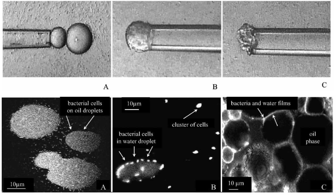
SOURCE: All images from Dorobantu et al. (2004).
is used to synthesize new macromolecules and biomass by using chemical energy for metabolism, with less energy lost as heat than in combustion.)
Aerobic hydrocarbon biodegradation occurs in oxygenated water, the uppermost layer of subsurface sediments, and intertidal beach sediments. Diffusion-limited seafloor sediments, wetland, estuarine, and fine-grained beach sediments and muddy tidal flats that are continuously anaerobic support various anaerobic processes. Because seawater has a relatively high concentration of dissolved sulfate, sulfate reduction is common in anaerobic marine environments, generating end products including hydrogen sulfide (H2S), hydrosulfide (HS–), elemental sulfur (S°), pyrites, and/or metal sulfide precipitates. Where sulfate is depleted, the energetically less-favorable processes of fermentation and methanogenesis can occur.
Aerobic microbes commonly degrade hydrocarbons without a partner species, and some exclusively metabolize hydrocarbons (obligate hydrocarbon-degrading bacteria; see Appendix I). In contrast, anaerobic hydrocarbon biodegradation, which currently is far less well understood, is often achieved through “distributed metabolism” (see Box 5.7) involving two or more species that are biochemically and/or physically linked, so as to overcome marginally favorable thermodynamic reactions. Aerobic hydrocarbon degradation is considered to be more rapid than anaerobic, and the known substrate range of biodegradable hydrocarbons is considerably larger under aerobic conditions. These factors are important for oil in the sea because it is relatively easy and fast for free-living aerobic hydrocarbon-degraders to begin metabolizing oil near the ocean surface within hours or days, but it may take weeks, months, or years for an anaerobic community to recruit and assemble suitable partners (physically and/or biochemically), then finally begin to biodegrade oil in anaerobic sediments, particularly when limited to fermentation and methane production. Lag times of several years have been observed for methane production from alkanes and aromatics in vitro (Siddique et al., 2015) but are unexplored in situ.
Degradation of methane provides a good example of contrasting microbial strategies: aerobic methanotrophs
(not to be confused with methanogens that are anaerobic methane producers) that are commonly detected near natural gas seeps consume methane without requiring other microbial partners. Conversely, anaerobic methane consumption commonly requires a slow-growing syntrophic partnership between two anaerobic members, for example, an anaerobic methane-oxidizing archaeon in close physical contact with a sulfate-reducing bacterium, forming a microscopic consortium (reviewed by Knittel and Boetius, 2009). These consortia tend to live in anaerobic sediments near natural seeps in the transition zone where the chemical gradients of methane gas and dissolved sulfate overlap (Knittel et al., 2005). Despite the extremely small energy yield of anaerobic methane oxidation, this activity in marine sediments exerts a major control over global methane flux from the ocean to the atmosphere (Reeburgh, 2007). Larger gaseous alkanes (ethane, propane, butane) released from subsurface gas seeps can be degraded aerobically by microbes other than methanotrophs. For example, Valentine et al. (2010) deduced that respiration of ethane and propane was an early driver of microbial response to the DWH event, and subsequent studies have suggested that Cycloclasticus, a bacterial genus previously thought to be an obligate PAH-degrader, may have utilized ethane, butane, and propane during active gas release early in the spill, then shifted to PAH degradation after the gas release ended (Rubin-Blum et al., 2017). Anaerobic degradation of non-methane gaseous hydrocarbons by sulfate-reducing marine bacteria has been observed both with (Singh et al., 2017; Chen et al., 2019) and without an archaeal partner (Kniemeyer et al., 2007).
In contrast to the special cases of gaseous hydrocarbons, biodegradation of liquid oil components is a widespread and well-studied phenomenon in marine systems, and metabolism of saturates and aromatics by diverse species has been known for decades (Van Hamme et al., 2003). The well-described aerobic biochemical pathways for saturates and aromatics differ. n-Alkanes typically are oxidized via beta-oxidation using pathways analogous to lipid metabolism, with fatty acids and alcohols as transient intermediates (Rojo, 2009). Neither n-alkanes nor their aerobic metabolites tend to accumulate in the environment or contribute to toxicity, and even highly branched pristane and phytane can be degraded by the ubiquitous species Alcanivorax borkumensis (Gregson et al., 2019) or depleted via co-metabolism (see Box 5.7) with long-chain n-alkanes (Deppe et al., 2005). Other iso-alkanes and cycloalkanes are less readily degradable, likely due to enzyme specificity, and suites of partially oxidized organic acids that fit the chemical definition of potentially toxic naphthenic acids (Clemente and Fedorak, 2005) may be produced and persist either in the oil or dissolved in surrounding water. In anaerobic systems fewer alkanes have been shown to biodegrade, the pathways are poorly known, and metabolites have proven difficult to identify and isolate (Mbadinga et al., 2011). Notably, anaerobic hydrocarbon research primarily has been done in terrestrial systems rather than marine sediments, but the processes are likely analogous. The anaerobic pathway for saturates requires activating the molecule via enzymatic addition of fumarate followed by beta-oxidation and central metabolism (Callaghan, 2013; Abu Laban et al., 2015; Jaekel et al., 2015). Under anaerobic but non-methanogenic conditions (e.g., sulfate reduction), a limited group of bacterial species is known to degrade alkanes without a partner. Until recently, hydrocarbon biodegradation under methanogenic conditions was thought to require the syntrophic association of a methanogenic archaeon with one of several bacterial species (reviewed by Gieg et al., 2014) as a complicated example of distributed metabolism (see Box 5.7). However, a methanogenic archaeon now has been inferred to oxidize long-chain alkanes and alkyl side-chains without a partner (Zhou et al., 2022).
Aromatic hydrocarbons are more chemically reactive than saturates, and numerous aromatics are mineralized or transformed aerobically by bacteria and eukaryotes (described below). Bacterial aerobic pathways for oxidizing (alkyl) monoaromatics and (alkyl)PAH are lengthy, sometimes requiring ≥14 enzymes (Elyamine et al., 2021) and usually involve addition of one or two oxygen atoms to the aromatic ring or the alkyl side chain, followed by ring opening and further degradation to alcohols, aldehydes, and carboxylic acids that can be funneled into central metabolic pathways (Jindrova et al., 2002; Haritash and Kaushik, 2009; Ghosal et al., 2016). However, the accumulation of polycyclic aromatic acids from partial biodegradation of alkyl-PAH may occur, with lower molecular weight metabolites (e.g., naphthoic acids) being transient but larger metabolites (e.g., fluorene carboxylic acid) persisting longer, especially if dissolved oxygen is limiting (Kristensen et al., 2021). The toxicity of such mixtures of aromatic acids to marine fauna is not yet known, as dilution in the water column or distributed metabolism may reduce any potential effects. In contrast to aerobic attacks, the anaerobic susceptibility of numerous alkyl-PAH is not yet fully known (Foght, 2008), nor are the substrate ranges for different types of anaerobic communities, although new ‘omics techniques are yielding some insights (Laczi et al., 2020). Some bacterial anaerobic pathways for aromatics require initial enzymatic activation via addition of fumarate, methyl, hydroxyl, or carboxyl groups prior to ring opening and/or saturation. Anaerobic depletion of alkanes, low-molecular-weight PAHs, and high-molecular-weight alkyl-PAHs in situ recently has been inferred from Gulf of Mexico deep-sea sediments (Bagby et al., 2016; Shin et al., 2019a), although the completeness of the oxidation is not known. Novel sulfate-reducing PAH-degrading bacteria and distinct metabolic pathways were discovered after the DWH spill (Shin et al., 2019a), indicating that we have yet to fully catalog the diversity of anaerobic oil degradation in the environment. Anaerobic biodegradation of hydrocarbons is not yet fully understood, and although the range of substrates is believed to be much narrower and more selective than for aerobic attack, general rules for anaerobic susceptibility have not yet been described. This hampers understanding and prediction of ecosystem recovery from oil that impacts seafloor sediments.
Eukaryotes, including some fungi and the organs of some animals, can biodegrade or transform hydrocarbons, exclusively aerobically. The biochemical pathways differ somewhat between prokaryotes and eukaryotes, with the former primarily being used for mineralization and cell growth and the latter being employed for detoxification purposes. That is, prokaryotic pathways have evolved to achieve maximum oxidation of the substrate for carbon and energy, whereas most eukaryotes only transform the hydrocarbon enough that it is less toxic and/or can be excreted because it has been made more water-soluble; alkane- and PAH-utilizing fungi are a notable exception. Importantly, some eukaryotic processes inadvertently increase hydrocarbon toxicity and carcinogenicity. The first steps of aerobic PAH oxidation are a good example. Bacterial enzymes commonly initiate aromatic degradation by introducing both atoms of O2 into the PAH structure via dioxygenase enzymes, some of which are quite substrate-specific and define the range of PAHs that each species can grow on. The products are funneled into central metabolism to be mineralized. Eukaryotes, in contrast, often use non-specific peroxidases or mono-oxygenases like P450 cytochromes (CYP1A; see Section 6.3.4.2) to oxidize hydrocarbons as well as other chemical classes including steroids, drugs, and carcinogens. Another eukaryotic option is glycosylation that chemically marks the compound for active excretion. Unfortunately, some transformed products have greater cell toxicity and/or carcinogenicity than the parent hydrocarbon and may accumulate as “dead-end” products that subsequently cause mutations or cell toxicity (Guengerich, 2008).
In summary, the ultimate outcome of combined aerobic and anaerobic oil biodegradation is the removal of most n-alkanes and monoaromatics and the depletion of selected iso- and cycloalkanes, PAHs up to five rings including certain alkyl-PAH isomers, and N-, S- and O-substituted aromatic resins (PACs). Bacterial attack with or without oxygen typically results in mineralization or substantial transformation of susceptible oil components to simple gases, biomass, and relatively innocuous water-soluble pathway products and may render the residual oil less acutely toxic. Aerobic eukaryotic metabolism may deplete some alkanes, mono-aromatics, and PAHs, with production and excretion of potentially toxic and/or carcinogenic products that can pass up the food chain.
Nutrient Availability
Efficient biodegradation requires sufficient nutrients to balance the high carbon content of oil (reviewed by Vergeynst et al., 2018). Water-soluble forms of nitrogen and phosphate are the most frequently measured bioavailable nutrients assessed for oil degradation and the Redfield ratio of 106:16:1 C:N:P (Anon, 2014) historically was used as a rule of thumb to estimate the N and P demand for efficient attenuation of oil spills (see Section 4.2.3.1 for discussion of bioremediation). Concentrations of dissolved nitrate, nitrite, ammonium and phosphate from terrestrial runoff may be adequate for oil biodegradation in near-shore waters and shorelines, but when these nutrients are sequestered into biomass (e.g., blooms of marine snow; see Section 5.3.2.2) they become less bioavailable, and dissolved concentrations may become limiting. Nitrogen compounds can be continuously supplied by some species of marine bacteria, particularly bacterioplankton that fix N2 gas, and by some N2-fixing heterotrophs that also degrade hydrocarbons (although seldom simultaneously; Foght, 2018). For example, N2 fixation by suspended particles in the Gulf of Mexico was substantial during the first few months after the DWH spill in parallel with methane consumption (Fernandez-Carrera et al., 2016), but it is not clear whether the same organisms were responsible for both activities simultaneously, or whether N2 fixation occurred aerobically (e.g., by cyanobacteria) or anaerobically (e.g., by consortia of archaeal methanotrophs and bacterial sulfate-reducers). In anaerobic seafloor sediments microbial nitrogen-cycling has been linked to PAH exposure (Scott et al., 2014). Thus, nutrient demand for oil degradation may be met by natural sources, and their concentrations generally are adequate, although not necessarily optimal, for hydrocarbon biodegradation in most marine environments.
Addition of exogenous nutrients (biostimulation; see Section 4.2.4) has long been known to enhance microbial activity and diversity in the presence of oil, as observed by in situ and in vitro experimentation, for example, in samples of Arctic and Gulf of Mexico surface waters (Sun and Kostka, 2019) and on beaches with sediment–oil aggregates (Shin et al., 2019b). Such amendment is justified only where permitted in locations where nutrients are limiting and amendments will not be diluted or washed away. Unfortunately, laboratory studies often provide nutrients at concentrations many-fold greater than the micromolar concentrations commonly available in situ, and therefore may generate unrealistic observations of activity and community response.
Trace elements including iron, copper, nickel, and rare earth elements (Shiller et al., 2017; Mehaja et al., 2019) may also be necessary for optimum biodegradation, functioning as co-factors for hydrocarbon-oxidizing enzymes.
Salinity
The salinity of seawater is sufficient to restrict microbial growth to species that are halotolerant, yet significant oil biodegradation is accomplished in the sea by microbes adapted to marine salinity. Higher salinity due to evaporation may occur in warm shallow coastal waters, wetlands, and beaches where it not only affects the composition of the microbiota but decreases water-solubility of some oil components, particularly PAHs, and limits biodegradation (Geng et al., 2021). Elango et al. (2014) determined that hypersaline conditions in the intertidal zone limited biodegradation of stranded tar balls, and Chen et al. (2010) likewise found that increasing salinity in mangrove sediments (from 5 to 25 ppt) decreased PAH biodegradation. Salinity may also be a factor in Arctic sea ice, where brine channels containing oil and microbes have higher salinity than the ice (see Section 5.3.5.3). Salinity gradients found in estuaries and
some continental shelf environments can influence petroleum compound solubilities (see Chapter 2, Section 2.1.5). This could interact with the aforementioned microbial species responses to salinity differences and have an overall influence on microbial degradation of petroleum compounds.
Temperature
Temperature is a factor in all microbial activities but distinct microbial communities are selected by and adapt to ambient temperatures where they perform optimally. They inhabit subsea hydrothermal vents, hot tropical beaches, temperate waters and wetlands, constantly cold deep-sea waters and sediments, and sub-zero polar sea ice, the latter being discussed in detail in Section 5.3.5. Biodegradation typically occurs over a range of ~30°C for individual species, with different communities prevailing over a sliding range from sub-zero to ≥60°C, given accompanying suitable conditions (reviewed by Margesin and Schinner, 2001).
Pressure
Hydrostatic pressure is an environmental co-stressor with low temperature in deep-sea water and sediments impacted by oil (reviewed by Louvado et al., 2015). Oil biodegradation was observed in the DWH dispersed plume at ~5°C and depths >1,000 m (Hazen et al., 2010) and oil biodegradation was inferred in seafloor sediments at ~2,000 m (Bagby et al., 2016). However, quantifying the effects of pressure on oil biodegradation is difficult because of the logistical challenges of sampling in situ and technical challenges of handling samples in the laboratory when simulating deep-sea conditions. This has hampered in situ and in vitro study of oil biodegradation, and our current understanding is very limited. Laboratory studies at high pressure and low temperature have varied considerably in their methodology, including the hydrostatic pressure applied (6–50 Mpa [megaPascal]) where 0.1 MPa is atmospheric pressure and 15 MPa corresponds to ~1,500 m depth). Some studies have used pure isolates or near-surface communities not previously adapted to pressure (e.g., Schwarz et al., 1975; Schedler et al., 2014; Scoma et al., 2016a), calling into question the relevance of the observations. Others have used piezotolerant microbial communities from geographically diverse deep waters (e.g., Prince et al., 2016a; Calderon et al., 2018; Marietou et al., 2018) or sediments (Calderon et al., 2018; Nguyen et al., 2018; Noirungsee et al., 2020) that necessarily were depressurized during sampling and manipulation, with unknown effects on cell viability before being repressurized. Some studies have amended the samples with pure hydrocarbons (Schedler et al., 2014; Scoma et al., 2016a) or a mixture of pure hydrocarbons (Calderon et al., 2018) whereas others used crude oil, either with (Prince et al., 2016a; Noirungsee et al., 2020) or without dispersant (Nguyen et al., 2018). Some studies have supplemented the cultures with nutrients (Schedler et al., 2014) and others have not (Barbato and Scoma, 2020); this is relevant because starving microbes may be more sensitive to oil and/or pressure.
Given the diverse parameters of these disparate studies, it is difficult to draw broad conclusions, but in general moderate pressure (6–15 Mpa) results in modest inhibition of oil biodegradation under laboratory conditions (Prince et al., 2016a; Nguyen et al., 2018), with different hydrocarbon classes possibly being more susceptible than others. Microbial community composition changes with pressure but the significance is not fully known. Notably, none of the studies have examined anaerobic biodegradation, which is most relevant in deep-sea sediments. Furthermore, although the solubility of hydrocarbons in liquid oil exhibits little variability with pressure, modeling predicts that high pressure may slightly increase water solubility, potentially increasing bioavailability and biodegradation. This contrasts with modeling of pure solid PAHs (not dissolved in oil) whose solubility decreases with increasing pressure (Oliveira et al., 2009). Unfortunately, measured effects of pressure on hydrocarbon solubility in seawater have not been reported in the literature, especially in combination with low temperatures experienced in the deep sea (Louvado et al., 2015). Understanding the synergistic effects of pressure, temperature, nutrients, oil type, and presence of dispersant will require improved experimental design using combinations of in situ and in vitro observations (Scoma et al., 2016b). Numerous gaps exist in understanding the effects of deep-sea conditions on aerobic and anaerobic oil biodegradation. The enormous volumes of deep waters and large areas of deep-sea sediments that may be affected by oil from natural sources and spills warrants the technical efforts that high-pressure studies demand.
Predation
Predation is a factor in all marine environments, affecting microbial communities and therefore oil biodegradation. Marine oil snow, for example, is a hotspot of microbial activity and therefore also concentrates microscopic predators (e.g., zooplankton) and bacterial viruses (bacteriophage; Suttle, 2007). The effects of predation, whether negative due to mortality or positive due to nutrient cycling, have not been rigorously studied, in part because they cannot be controlled during in situ experiments or faithfully replicated in vitro.
To summarize Section 5.2.8.8, no single environmental factor controls oil biodegradation in the sea. Rather, unique combinations of factors that reflect the specific environment and abiotic weathering progression, in concert with the microbial community composition and oil characteristics, influence the ultimate rate and extent of oil biodegradation in the sea.
5.2.9 Examples of Oil Spill Budgets
As demonstrated in Sections 5.2.1–5.2.8, oil in the sea experiences multiple fates depending on its composition, the site, prevailing conditions, and timeline. Section 5.2.9 describes how the various fates can be assigned proportions during a spill. This bridges Section 5.2, which describes fundamental processes
affecting oil fate irrespective of the site, and Section 5.3 that describes oil fates in specific marine environments. At a fundamental level, an oil spill budget reports the amount of spilled oil entering different environmental compartments (e.g., water column, sediments, sea surface, atmosphere, etc.) and being removed or altered by different fate processes (e.g., dissolution, biodegradation, volatilization, etc.). Spill budgets are developed for different purposes at different times, each dependent on different amounts and quality of data. The definition of the various compartments and processes should be suited to the purpose of the budget. Early during a spill, the main purpose of a spill budget is to direct the response and inform the public and decision makes. Following a spill, budgets are determined through the NRDA process as part of the penalty assessment. During and following a spill, detailed scientific budgets may also be developed to support research. Here, we give a few examples of spill budgets, their uses, uncertainties, and variability.
5.2.9.1 Caveats on Oil Budgets
During an oil spill response the Unified Command, stakeholders, and general public require reporting on the mass balance/oil budget from mitigation activities and natural processes. These spill accounting volumes help estimate the percentage of cleanup completed and how much is left to respond to. It helps measure the pace of response activities and gives a sense of how long the incident will take to resolve. Under the Incident Command System, Form 209 collects these data. Amounts entered include volume spilled/released, recovered oil, evaporation/airborne, natural dispersion, chemical dispersion, burned, floating contained, floating uncontained, onshore, and total oil accounted for. As will be seen in the discussion below, each of these volume categories has a wide range of potential values, so the oil budget is never an absolute single number, but generally represented by a range of values.
Oil budget calculations for a particular incident may include:
- initial amount and type of oil released (if known);
- amounts remaining as floating, evaporated, naturally dispersed, and/or beached oil;
- amounts removed—by collecting at the source, skimming oil from the water, chemically dispersing the oil (if used), and/or in situ burning (if used); and
- amount of oil recovered from the shoreline.
As described in Chapter 2, oil is a mixture of many different chemicals, with varying toxicity and behavior in the environment which can affect the behavior of the oil itself. When oil spills, several factors determine how the oil will behave, how the oil will interact with the environments, and the eventual fate of the oil:
- The volatility of the oil components determine how quickly the oil will evaporate when spilled.
- Oil components that are more soluble in seawater will partition more to the water phase.
- The biodegradability of the oil will determine how easily the oil is broken down by microbes.
- Sunlight can transform oil components.
- Chemical changes in the oil affect the physical features like density and viscosity.
These physical and biological processes results in what is referred to as the “weathering” of the oil. Weathering describes changes in the oil’s chemical composition and physical characteristics over time.
While laboratory studies of oil weathering processes can be rigorously performed, studied, and measured to very precise percentages of the different weathering compartments, extrapolating controlled laboratory measurements to field conditions is not possible to the same degree of precision due to the heterogeneity of the ocean and degree of uncertainty of each of the input categories. In a laboratory the initial conditions (input quantity, type of oil, temperature, agitation, etc.) can be strictly controlled and measured. These data can be incorporated into mathematical algorithms that are used in computer models to estimate weathering in the field. The programs may provide a “best guess” answer and are designed to run on as little information as possible, especially using the type of information that can be estimated quickly or obtained in the field. The programs may incorporate environmental properties such as salinity and temperature of the water, wind speed, and/or wave height. Spill properties include the type of oil spilled along with the rate and duration of the release. Spill properties may be very uncertain, especially early during a spill. Hence, it is valuable to remember the general rule of thumb with any computer modeling program: “Garbage in = Garbage out.” Hence, the greater the uncertainty of your data inputs, the greater the uncertainty in your model outputs.
For many incidents it is very difficult to measure the exact amount of oil initially released; this estimate affects subsequent calculations. The composition of the spilled fluids may also be uncertain. Thereafter, one of the greatest uncertainty inputs for calculating an oil budget lies in the weather conditions and forecasts, both in time and space. Whereas, in a laboratory you can control the wind speed, duration, and temperature, in the field these are changing moment to moment and from location to location.
Due to the heterogeneity of environmental conditions and oil properties, some portions of the slick will form a sheen, naturally disperse and evaporate, and some portions will stay thick and emulsify. Ocean circulation may concentrate some of it and dissipate other areas. Mass balance calculations would ideally identify 100% of the oil spilled. In fact, some processes (physical recovery and biodegradation) eliminate oil, and some others—such as emulsification—increase the volume of the slick floating on the surface, which is the oil that is being observed, measured, and recovered. Therefore, the volume of the petroleum product is constantly changing in both competing directions, as it incorporates water or loses components, resulting in the slick areas varying significantly. The amount of oil stranded on a shoreline is also extremely
varied in thickness (quantity), and calculations attempt to average out these volumes over the distance covered.
In general, evaporation is very well understood and can be fairly well extrapolated to field conditions. Dissolution is next in line with a fairly high degree of confidence from lab studies as it is related to the amount of “light ends” (low-molecular-weight components) in the parent oil, as is evaporation. In the subsurface the problem increases three-dimensionally as the currents are not well characterized and we are not able to directly see the oil so that it is difficult to track, and there is also the difficulty of predicting the droplet size distribution. Estimates of natural dispersion and droplet formation are very uncertain as they depend significantly on the energy from wind and waves on the surface being transferred to the floating oil. Although natural dispersion and droplet formation are mechanisms that remove oil from the water’s surface, this is not truly a weathering process in terms of any chemical transformation—it is more of a transport mechanism with the oil remaining physically the same, just in smaller droplets. Additionally, naturally dispersed oil droplets may recoalesce at the water’s surface when wind and turbulence decrease. Emulsion formation prediction is probably the least reliable calculation as it too is related to the type of parent oil and the physical energy it encounters in the field, with the physical mechanism of action greatly different from laboratory waves to real ocean waves. Running many statistical analyses to compute the uncertainties and reduce them with comparisons to real-world observations is one method to help produce a “best guess” estimate to within an order of magnitude.
Oil budgets are produced by experts in their fields using the best available data for input into calculations and models. This is followed by a process of comparing the calculated results with observable situations and finding approximate fits to the solutions. There is almost always a spread in the results and through a process of informed negotiations and best professional judgement consensus on the closest approximations of the range of results is issued. Oil budgets should be viewed as scientifically derived qualitative information rather than precise numbers for the oil volume partitioning between different compartments. There are many challenges described in this report related to the estimation of the released volume, oil volume present on the water surface, as well as estimations of weathered and recovered oil volumes sited in the mass balance table. The focus on these numbers without proper understanding of associated uncertainties has created issues, misunderstandings, and delays during past responses and exercises. The response community is encouraged to describe a changing spill situation by focusing on the objective and verifiable numbers important for response and impact assessment. For example, surface area affected by the spill that can be estimated and documented using remote sensing techniques or the length of the affected shoreline that could be estimated and documented by SCAT programs assisted with remote sensing if needed.
One example of a computer system to estimate oil movement and weathering is NOAA’s WebGNOME trajectory modeling software (see Figure 5.19). ADIOS2® (Automated Data Inquiry for Oil Spills) is the oil weathering model component. It is an oil spill response tool that models how different types of oils weather (undergo physical and compositional changes) and calculates the amount of evaporation, floating, dispersion, sedimentation, water content, density, and viscosity of the oil in the marine environment. Working from a database incorporating laboratory data of more than a thousand different crude oils and refined products and given an estimate of the composition of a spilled oil, ADIOS2 quickly estimates the expected characteristics and behavior of spilled oil (NOAA, 2021c).
Properties compiled in the database include the density, viscosity, and water content of an oil or refined product, and the rates at which it evaporates from the sea surface, disperses into the water column, and forms oil droplets that become emulsified, or suspended, in the water (NOAA, 2021c). The database was compiled from a variety of sources, including Environment and Climate Change Canada, the U.S. Department of Energy, and industry. The predictions are designed to help decision-makers develop cleanup strategies. All of the outputs need to be understood with the limitations to precision and the range of variability there may be from the low to high estimates. Quoting from the WebGNOME manual, “Uncertainty is the only certainty there is.”
5.2.9.2 Exxon Valdez Oil Spill Budget
From the report by Wolfe et al. (1994) (see Figure 5.20), it is estimated that over time by day 1,000+:
- 11% of spilled oil was estimated to remain in the sediment
- 5% had been stranded on beaches
- 12% had been mechanically recovered
- 2% was dispersed in the water column
- 50% had been biodegraded (to an unknown degree)
- 20% had evaporated or photo-oxidized
It can be seen in the graph that over time the estimated percentages of each compartment varied. Evaporated and photolysis products were a continuing process throughout the incident. Floating oil was gone about two months after the initial release. Oil recovered or disposed of began soon after the release and grew throughout the response. Biodegradation products started within the first month and continued throughout. Naturally dispersed oil peaked in the first month and then waned. Oil incorporation into the sediments occurred after a few months and then continued. The graph does not show any ranges in the values on the estimates for each compartment that do appear in the text of the report.
5.2.9.3 Deepwater Horizon Oil Spill Budget
These estimates were supplied as part of the oil budget: Oil Budget Calculator Technical Documentation (2010), a peer-reviewed report over 200 pages that presented the formulas used and updated the percentages in the original budget (see Figure 5.21).
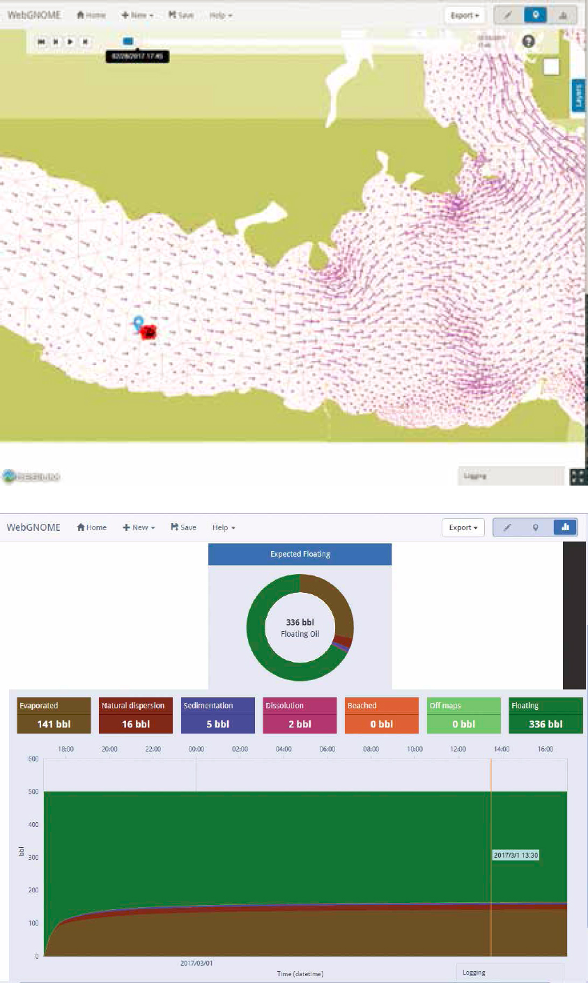
SOURCES: NOAA; ADIOS (2021).
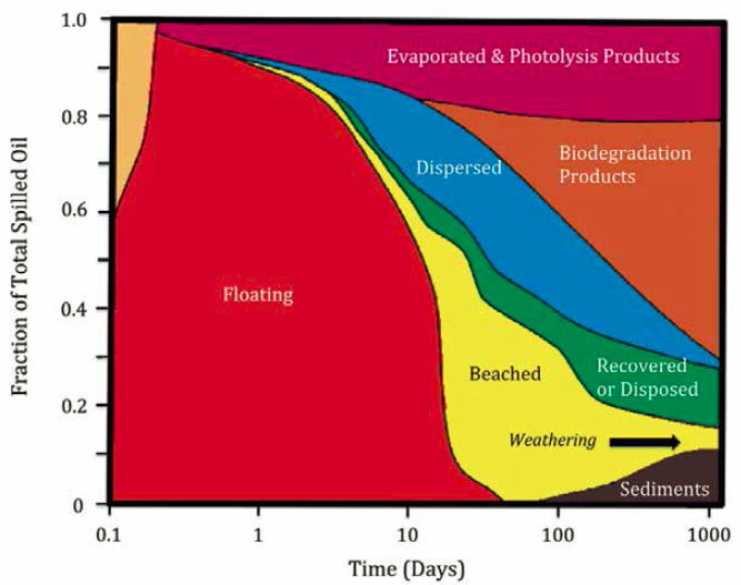
SOURCE: Reprinted with permission from Wolfe et al. (1994). Copyright 1994, American Chemical Society.
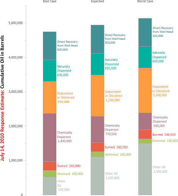
NOTES: These estimates served solely as a guide for the national response to the DWH MC252 gulf incident. The best and worst cases defined in the report are the combinations of values of the seven variables depicted in each stack that correspond to the lower and upper endpoints of a 95% confidence interval for the volume of “Other Oil.” The Oil Budget Calculator does not quantify the volume of oil that forms tar balls or surface slicks, sinks due to sedimentation, remains in the surf zone, or impacts the shore and is subsequently cleaned up. These are instead grouped together as “other oil.” The amount of oil listed as “other” is quite large in the DWH oil budget.
SOURCE: Federal Interagency Solutions (2010).
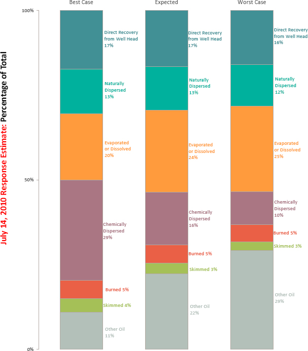
SOURCE: Federal Interagency Solutions (2010).
The oil budget (see Figures 5.22 and 5.23) indicated that response and containment operations collected, eliminated, or dispersed in the expected case about 41% of the oil, with containment (“direct recovery from wellhead”) being the most effective method, and chemical dispersant applications at surface and subsurface dispersing a substantial fraction (National Commission, 2011a). Subsurface application of dispersant resulted in dispersion of the oil before it reached the surface, limiting the amount of surface oil that could be skimmed, burned, or dispersed at the surface. Roughly 8 percent of the oil in the expected case was removed through skimming or burning, with burning operations considered to be more successful than skimming despite the resources directed to skimming operations (National Commission, 2011a). Comparing the three cases—best, expected, and worst—it can be seen that the results may vary several-fold, depending on the assumptions.
Lessons Identified by the Federal Interagency Solutions Group (2010, p. 38):
The experience in developing the calculator pointed to areas needing future research and planning:
- Protocols for surface and subsurface sampling: While oil samples were collected for impact assessment, few samples were properly collected and categorized for response.
- Dispersed oil droplet size: A major improvement in estimating dispersant efficiency would be possible if practical operational tools and methods existed to characterize droplet size distribution of subsurface oil.
- Basic models for longer-term processes: While longer-term processes such as biodegradation often happen outside the time frames of the response, understanding and being able to predict such longer-term changes may be useful in making response decisions.
- Estimation of collected shoreline oil: For a complete mass balance, procedures should be implemented that estimate the fraction that is oil on the oiled debris gathered from shoreline cleanup.
- Expanded modeling capabilities: Many of the team members that assisted with the Oil Budget Calculator were also part of a working group of spill experts developing the specifications for the next generation of oil spill model. These specifications need to be translated into real code.
- Revised interface: A better interface is necessary to more properly display the intrinsic uncertainty in the calculator.
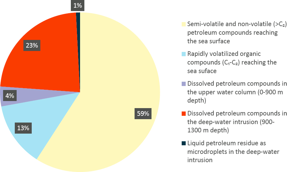
NOTES: The shaded regions report the percentages of the total discharge resident in each category and environmental compartment (see inset legend for details). Simulation results are for the base-case scenario of the most likely fate with the applied subsea dispersant injection of June 8, 2010.
SOURCE: Gros et al. (2017).
Gros et al. (2017) and French-McCay et al. (2021a) reported mass balance predictions for the DWH oil spill based on oil fate and trajectory modeling (see Figures 5.23 and 5.24). The authors report the mass balance for the fate of fluids discharged to the ocean water column, not including the fluids collected directly at the wellhead. Gros et al. (2017) reported fates for different compound groups and environmental compartments and performed simulations only for June 8, 2010; French-McCay et al. (2021b) analyzed the total mass entering each environmental compartment. From Figure 5.23, Gros et al. (2017) reported that 72% of the petroleum released on June 8 reached the sea surface, 13% of which rapidly volatilized to the atmosphere, 27% dissolved into the ocean water column, and about 1% became trapped in the water column as tiny oil droplets. From Figure 5.24, French-McCay et al. (2021b) reported, up to June 8, 2010,
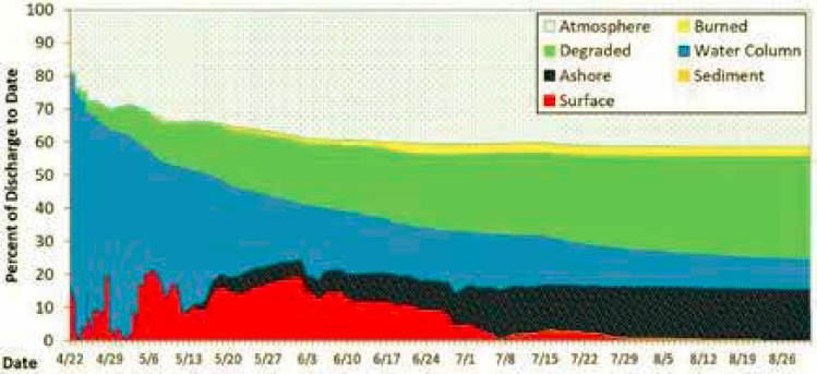
NOTES: The shaded regions report the percentage of discharge represented in each environmental compartment over time (see inset legend for details). Simulation results are for the base-case scenario of the most likely fate. This is the only model that considered biodegradation; the model did not consider photo-oxidation.
SOURCE: French-McCay et al. (2021b). CC-BY ND.
that 14% of the petroleum discharged since April 22, 2010, was floating on the sea surface, 8% had stranded ashore, 17% had become trapped in the water column, 20% had been biodegraded, 2% was burned, and 39% had partitioned to the atmosphere. Figure 5.24 also shows that this partitioning varied in time as different intervention methods were applied and because the various fate processes have different time scales.
As can be seen by these different approaches to calculating oil budgets: it is difficult to compare different types of calculations and models; there are very large/rough/round numbers used; the “Other” category may encompass a large volume and vary in definition; there are many different combinations of ways to view the numbers (not every assumption will hold true for low, mean, high supposition—some may be high, some may be low, etc.); the results may differ by millions of gallons or be “unaccounted for;” and the time scales vary for each scenario.
5.2.9.4 M/T Athos I Oil Budget
During the M/T Athos I (see Box 4.1) response, the Unified Command requested the Environmental Unit to calculate a mass balance/oil budget for the recovery activities. As can be seen in Figure 5.25, there is a wide spread in the values calculated depending on the assumptions made, as there were very few absolute values to use. The most reliable number was the total amount released, as that was able to be calculated from the volume loaded into the hold and the amount pumped out after the spill. This number was also rounded to the nearest thousand. Due to the complex system that the oil was released into, the resultant calculations are highly variable in space and time. Each of the categories in the table show a wide range of values except for evaporation, as there was consensus that this particular heavy oil had negligible light ends and therefore nearly zero evaporation.
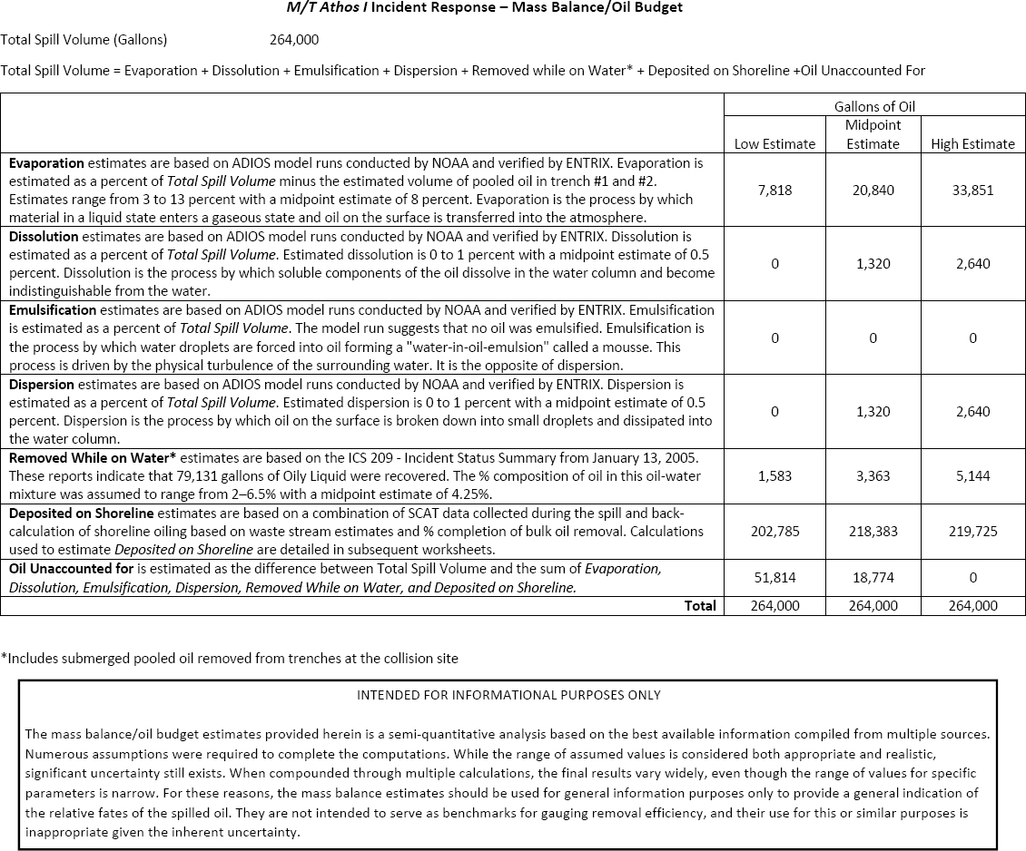
NOTE: This is intended for informational purposes only.
SOURCE: Levine, E. Unpublished data.
Depending on the assumptions for each variable, the remainder in the “oil unaccounted for” varies greatly (from 20% to 8% to 0%). These calculations have merit for framing the pace of the response, but not as an absolute accounting.
5.3 OIL FATES IN SPECIFIC MARINE ENVIRONMENTS: EPISODIC INPUTS
Section 5.2 introduced the fundamental parameters and processes influencing the fate of oil including slick formation, gas bubble and oil droplet breakup, and dispersion, regardless of geographic location and marine system. In Section 5.3 we use these universal mechanisms to describe how the properties of specific marine systems affect the fate of oil from episodic inputs (i.e., typically single, finite events). Section 5.4 considers chronic inputs.
This section begins by describing oil in surface and near-surface waters (to ~10 m depth); then in the underlying water column from the photic zone (up to ~50 m depth) and below (<1,000 m depth); then deep-sea waters and sediments (>1,000 m depth); and finally oil-impacted shorelines including beaches and estuaries. The fate of oil in the Arctic is presented as a special case.
5.3.1 Sea Surface Processes Affecting Oil Fate
Oil may reach the ocean surface either directly as a surface spill or from a subsea petroleum source. This section addresses processes immediately at the ocean surface or originating at the ocean surface and potentially affecting transport over the upper mixed layer of the ocean, extending to depths of order ~10 m. Most oils are lighter than seawater, so newly spilled oil tends to rise toward the surface and accumulate, at least temporarily, where it is affected by a wealth of weathering and transportation processes. Oil floating at the sea:air interface is exposed to the atmosphere, where it may evaporate or photo-oxidize, and also interacts with the near-surface water column, where it may be dispersed or dissolved. Wind and waves together with ocean currents transport the oil and may promote dispersion of the oil from a floating slick to submerged oil droplets or emulsions. These processes are described in the sections below.
5.3.1.1 Initial Spreading of Oil on Surface Waters
Oil at the surface initially spreads under gravitational forcing to form a slick or sheen. In the open ocean, where there are no physical boundaries, oil spreads out by gravitational forcing and eventually pools in slicks and sheens (described in detail in Section 5.2.2.1 and Figures 5.3–5.5). These layers of oil can be extremely thin, approaching a thickness of a few micrometers. Gravitational spreading typically is important on length scales of meters to hundreds of meters and ceases when the interfacial tension of the oil layer begins to resist further spreading. After initial spreading, wind and wave action may cause the oil to undergo dispersion, evaporation, dissolution, or emulsification. Importantly, oil floating at the surface is more susceptible to photo-oxidation than submerged oil (see Section 5.2.5). The ultimate fates of various photo-oxidation products (whether via dissolution, sedimentation, biodegradation, etc.) are not yet fully known, but amphiphilic photo-oxidation products that increase hydrophobic interactions and aggregation of oil droplets (by altering surface activity or stickiness) can enhance both emulsification (Ward et al., 2018a; Ward and Overton, 2020) and the formation of marine oil snow, discussed below (see Section 5.3.2.2). In contrast to photo-oxidation, oil slicks are less susceptible to biodegradation than submerged oil droplets because the surface area available to microbes is smaller in a slick for a given oil volume (Prince and Butler, 2014).
There is a significant knowledge of the accumulation of natural organic material such as biosynthesized lipids, natural marine biopolymers (e.g., exopolymeric substances; see Section 5.3.2.2) and natural surfactants in oily-like surface films at the air-sea interface. The physical chemical properties of these substances indicate that such materials will also accumulate with petroleum oil slicks and films. Human synthesized and human mobilized contaminant/pollutant chemicals with physical chemical properties such as chlorinated pesticides, polychlorinated biphenyls, and other persistent organic pollutant and organic pollutants of emerging concern with physical chemical properties similar to petroleum compounds are likely to be partitioned into the petroleum oil slicks. Discussion of these interactions and subsequent fates and effects is beyond the scope of this report.
5.3.1.2 Wind Drift and Stokes Drift
Oil transport modelers have observed for decades that floating oil tends to move by a combination of the near-surface ocean currents and the wind vector. This added velocity component from the wind is called wind drift; typical values are in the range of 1% to 3% of the wind velocity. It is also well known that there is a nonlinear component of the surface wave orbital velocity that contributes a non-zero net transport. This wave effect is known as Stokes drift, and its direction and magnitude are a function of the surface wave energy spectrum (D’Asaro et al., 2020). Oil floating on the sea surface or suspended within the orbital velocity field of surface waves will be acted on by wind drift and Stokes drift. Stokes drift can be included through analytical expressions; wind drift depends on the mechanisms causing its effect.
The motion within a surface oil slick will be in balance with the water and wind forcing so that the friction, or shear stress, experienced on either side of the oil–water or oil–air interfaces is the same. For relatively thick surface oil, this means that the shear stress between the air and oil could differ from that between the oil and water so that the wind could accelerate the oil separately from the acceleration transferred to the water column. Surface texture of thick oil layers could also result in different stresses applied to the oil and water. Either effect could cause a wind drag on the oil that pushes the oil in the downwind direction, adding a wind drag to the oil transport and causing the oil not to purely follow the surface ocean currents.
Another mechanism explaining the apparent wind drift derives from the variation of current velocity with depth in the near-surface of the ocean. At the air–water or air–oil interface, the friction, or shear stress, on the water or oil side of the interface will be equal to that applied by the winds. Moving away from the air–water or air–oil interface, currents will adjust to match general ocean currents at depth that may not be aligned with the winds. In the oceans, this adjustment will further occur in the surface Ekman boundary layer, the region coupling the rotation-dominated ocean interior, which may be in geostrophic balance with currents perpendicular to the pressure gradient, to the surface boundary conditions, in which currents are parallel to the pressure gradient. Because of these competing dynamics, recent measurements in the northern Gulf of Mexico (Laxague et al., 2018) confirm that significant velocity shear may be confined to the upper few centimeters of the ocean surface. Numerical models of ocean circulation must solve for very large domains so that the upper-most cell of a numerical model may be of order 1 m or more in depth. While numerical simulations are likewise in equilibrium with the applied surface stresses, they integrate these fine-scale variations in currents over a comparatively large depth. Because oil slicks are very thin, oil is likely to always be transported at the same speed as the real ocean currents at the sea surface. However, because numerical models predict average currents over a relatively thick surface grid cell, fine-scale effects of the winds need to be added to the oil transport floating on the top of these grid cells. Because ocean circulation models typically resolve the surface layer with similar order-of-magnitude length scales, the wind drift factor of 1% to 3% of the wind is a fairly stable parameter in oil trajectory modeling. As ocean circulation models become more resolved or include subgrid scale parameterizations for the surface boundary layer, the wind-drift parameter may become less important or eliminated altogether. Hence, apparent wind drift is an artifact of low model resolution at the air–water interface that generally should adapt to the resolution of the model as circulation models improve.
5.3.1.3 Natural and Chemical Dispersion of Oil in Near-Surface Waters
Entrainment of oil from the sea surface into near-surface water occurs when oil droplets separate from the oil slick and enter the water column—a process commonly referred to as natural dispersion when dispersants are not used and chemical dispersion when they are used (NASEM, 2020) (see Box 5.4 and Section 5.2.2.4). Oil entrainment is caused naturally by surface mixing via wind, waves, and currents and can be enhanced by the application of chemical dispersants. When floating oil is dispersed, its surface area to volume ratio increases, providing greater interaction of oil with seawater and allowing other natural processes to occur at faster rates (e.g., dissolution, biodegradation). To the extent that these oil droplets shade others or become dispersed below the photic zone, photo-oxidation for entrained oil may be reduced or arrested (Xiao and Yang, 2020).
The processes of dispersion of oil are complex. Floating oil may form submerged oil droplets when fluid motion at the oil–water interface entrains oil below the sea surface and turbulence in the upper mixed layer of the ocean breaks the entrained oil into droplets of various sizes. Whereas larger oil droplets can rise back to the water surface, smaller droplets remain in suspension in dispersed form in the water column. Entrainment of oil floating on the sea surface into the ocean interior requires both downward currents and encapsulation of oil within these currents. Breaking waves are the most notable source of entrained oil (Delvigne and Sweeney, 1988). Oil entrainment has also been observed for regular, non-breaking waves (Li et al., 2008), and may result from downwelling between the windrows of Langmuir circulations. Langmuir cells consist of alternating rows of helical vortices resulting from nonlinear interactions of the winds and waves (Yang et al., 2015). These complex processes set the source rate of oil entering the upper ocean turbulence. Turbulence within this domain also depends on a range of processes occurring near the air-water interface. These include wind stress at the sea surface, wind-induced currents, currents and turbulence resulting from ocean circulation, a broad spectrum of breaking and non-breaking waves, and Langmuir circulations (D’Asaro et al., 2020). Turbulence within this complex system is highly variable in space, and turbulence generated by periodic forcing, such as waves and wind gusts, can be heterogeneous and intermittent, resulting in strong temporal variability. Hence, breakup of oil droplets or gas bubbles in the upper ocean is a complex process, highly variable in both space and time, dependent on the local wind and sea state and on the oil properties of viscosity and surface tension, which set the interaction dynamics between entrained oil and the ocean currents and turbulence.
The entrainment rate of oil as droplets is faster for light oils with low viscosity and low interfacial tension. Sometimes chemical dispersants are sprayed on floating oil to reduce interfacial tension and promote dispersion. Low air and water temperatures, as well as most weathering processes, increase the viscosity of oil, thereby reducing the rate of natural dispersion. The rate of natural dispersion may also decrease with increasing ice coverage. The presence of ice on water reduces water surface and wave activity; thus, mixing and energy dissipation could be very low. Ice coverage may also reduce the interaction of oil with the atmosphere. Together, these processes may slow weathering, allowing fresh oil to persist longer. Interactions of oil with ice are complex and how oil is dispersed under partial or complete ice coverage remains a major challenge for predicting oil trajectories during response.
Classical understanding of natural oil dispersion from the sea surface originated with Delvigne and Sweeney (1988), who showed, based on small- and large-scale laboratory experiments, that floating oil could be entrained as droplets
due to the effect of breaking waves on the sea surface. Their measurements in two laboratory wave flumes showed two important conclusions. First, surface oil is entrained to a characteristic depth that depends on the wave height at breaking. Second, the maximum droplet size observed within the entrained oil depends on the characteristic depth of oil entrainment, the rise velocity, or slip velocity, of the formed droplets, and the time since wave breaking. Some of the entrained oil failed to break up into small droplets and rose to the sea surface nearly immediately following breakup. As the time since breaking increased, the droplet sizes remaining in the water column, therefore, decreased. Delvigne and Sweeney (1988) further related the volume flux of entrained oil per unit area of the ocean to the dissipated breaking wave energy per unit surface area and the fractional coverage of the sea surface by oil and by breaking waves. Though these correlations are highly empirical and must be fitted to each type of oil, the general understanding remains valid: Breaking waves entrain oil to a characteristic depth, and droplets remaining in the water column must be small enough not to resurface in the time between breaking events.
Recent insight on natural dispersion of oil by waves grew out of new experimental techniques that allow measurement of the in situ turbulent kinetic energy dissipation rate and the evolving oil droplet size distribution. An important set of experiments using regular and breaking waves and involving oil and oil plus dispersant were conducted by Li et al. (2007, 2008, 2009a,b,c, 2010). This work and other historical contributions are carefully reviewed in the more recent experimental work of Li et al. (2017). The Li et al. (2007, 2008, 2009a) studies showed that, while breaking waves are much more effective at dispersing surface oil, oil entrainment does occur under regular, non-breaking waves. They also showed that chemical dispersants can significantly reduce the droplet sizes of oil droplets forming under waves and increase the volume of entrained, dispersed oil. Through their laboratory measurements, Li et al. (2008) introduced a model that they refined in Li et al. (2009b,c) for the kinetics of oil droplet breakup under waves. They also quantified the effects of the turbulent eddy dissipation rate under waves. The focus in these studies was on the droplet size distribution. Li et al. (2010) used oil concentration measurements to further define the dynamic dispersant effectiveness, which is a measure of the mass fraction of oil suspended in the water column a certain time after a wave passage or breaking event. Using results for a heavy fuel oil, they concluded that less than 15% of the oil is dispersed at low temperature (<10°C) or for non-breaking waves; whereas better than 90% efficiency could be achieved using chemical dispersants at 16°C. This illustrates the importance of oil properties, especially viscosity and surface tension, and the surface flow dynamics, including wave characteristics, on dispersion of oil from the surface ocean. Li et al. (2017) used cutting-edge fluid dynamics observations to further elucidate the dynamics of oil droplet formation under breaking waves with and without chemical dispersant addition. They quantified the turbulent eddy dissipation rate in space and time for various laboratory simulations of deep-water breaking waves and measured the dynamic oil droplet size distribution. During the breakup process, they did not observe any coalescence events but did observe two forms of droplet breakup. Larger droplets form by primary breakup caused by the droplet-scale turbulence. When dispersant is added, droplets further undergo tip streaming, resulting in long micro-threads of oil which eventually break up into micron- and submicron-sized droplets (Gopalan and Katz, 2010; Davies et al., 2019).
Because Li et al. (2017) directly measured the time-evolving turbulence field, these measurements could also be compared to droplet size predictions using the Hinze (1955) model. Using the theory expressed in that paper (specifically, Equation F.1 in Appendix F), Li et al. (2017) showed good agreement between predicted and observed maximum droplet sizes in most experiments when using initial values of turbulent fluctuating velocities observed immediately following wave breaking. This is in agreement with their observation that larger droplets form rapidly by primary breakup in the turbulent field of the breaking wave. Li et al. (2017) also applied the Hinze theory using empirical relations for turbulent eddy dissipation rate under the roller of a breaking wave. These likewise showed good agreement in most experiments with the observed maximum droplet sizes. These Weber-number type predictions following Hinze (1955) are less accurate for the experiments with high dispersant to oil ratio (e.g., 1:25). In those experiments, it was more difficult to identify the characteristic droplet sizes in the measurements, and breakup by oil threads via tip streaming becomes important—a process that does not depend on the turbulent dynamics of the breaking wave and is not predicted by the dynamics described by Hinze (1955). Hence, when breakup occurs by turbulent eddies, predictions using the Hinze (1955) analysis do agree with observations, but when surface tension is low, as following chemical dispersant addition, other processes of droplet breakup dominate.
Two recent empirical equations (Johansen et al., 2015; Li et al., 2017) attempt to predict the droplet sizes of naturally dispersed oil. Both are based on an approach similar to that of Wang and Calabrese (1986) in which both Weber number and viscosity groups are involved and where the droplet-scale turbulence is parameterized by bulk, flow-scale variables. Johansen et al. (2015) define a modified Weber number, following the approach of Johansen et al. (2013), in which a bulk Weber number and viscosity number are combined. In their approach, the characteristic length scale is the oil slick film thickness, and the turbulent eddy dissipation rate is considered proportional to the kinetic energy of the breaker. In the Li et al. (2017) approach, they combine a bulk Weber number with the Ohnesorge number, another non-dimensional parameter that compares viscosity effects to surface tension forces and here, equivalent to the Hinze (1955) viscosity group. In their equations, the characteristic
length scale is taken as the maximum stable droplet size for a drop rising in quiescent water (Clift et al., 1978). Both of these equations show good agreement with measured droplet size distributions after calibration of their fit parameters. The Li et al. (2017) approach was explicitly calibrated for experiments with and without dispersant. The Johansen et al. (2015) approach, though appropriately including the viscosity number, has not yet been validated to experiments with chemical dispersant treatment. Overall, these approaches appear promising for predicting droplet size distributions for natural dispersion of oil at the air–sea interface.
The transport of dispersed oil in the upper mixed layer of the ocean is also a complex process. Cui et al. (2018) simulated transport of oil droplets under a deep-water breaking wave, and Cui et al. (2020a,b) coupled the under-wave transport with a population balance model for predicting the oil droplet size distribution. The advection and dispersion field within the region affected by wave breaking is highly heterogeneous and complex, containing downwelling currents, entrained air and oil, and highly fluctuating vorticity and eddy dissipation fields, among other complex processes. These affect oil dispersion in two key ways. First, the heterogeneous turbulent field-controlled droplet breakup. Second, the non-uniform turbulence and current velocity fields create non-uniform diffusivity fields. To model the transport of oil droplets using a Lagrangian particle tracking approach in a non-uniform diffusivity field requires a random displacement model (Boufadel et al., 2018; Cui et al., 2020b). Sophisticated laboratory data (e.g., Li et al., 2017) and numerical simulations (e.g., Cui et al., 2018, 2020b) are helping to understand these processes and develop appropriate field tools. At the same time, little field-scale data are available to study the dispersion process or to validate models that predict droplet size distributions under different dynamic ocean conditions.
5.3.1.4 Other Processes Affecting Surface and Near-Surface Oil
Photo-oxidation, dissolution, evaporation, emulsification, and biodegradation affect oil at and near the water surface, and have been described in detail in Sections 5.2.3–5.2.8. Photo-oxidation is most effective at the surface and rapidly diminishes with water depth, refraction off suspended particulates and self-shading by dispersed droplets. Thus, slick thickness, suspended sediment content, and depth of dispersed oil in the water column affect the impact of photo-oxidation. Dissolution occurs between the petroleum–water interface of surface floating oil and suspended water droplets. Because evaporation is faster than dissolution, dissolution is less significant for predicting the mass balance of surface, floating oil slicks. However, natural dispersion and dissolution from the suspended oil droplets together remain a similar order of magnitude to evaporation, and should be considered (MacKay and Leinonen, 1977). Natural dispersion is assessed as described above, and dissolution is analyzed using the approaches described in Section 5.2.5 for suspended bubbles and droplets. Emulsions arise through physical forces but may be enhanced by biological polymers and stabilized by microbial cells and/or their extracellular products (see Section 5.2.8.3). Whereas oil-in-water emulsification may increase the interfacial area available for biodegradation, particularly in the case of naturally produced microbial biosurfactants (Ron and Rosenberg, 2002), water-in-oil emulsification may decrease biodegradation due to limited diffusion of nutrients in seawater to the interface of internal water droplets. As previously discussed, biodegradation of near-surface oil is likely to be exclusively aerobic (see Section 5.2.8.8), and any predation of oil-degrading microbial blooms by predators and grazers (viruses, zooplankton) may decrease the rate of biodegradation of oil components. The role of marine oil snow in oil sedimentation and biodegradation is discussed in Section 5.3.2.2.
Oil chemistry affects the fate of surface oil. Notably, little is known yet about the in situ weathering properties of low sulfur fuel oils (LSFOs) and very low sulfur fuel oils (VLSFOs), new classes of marine fuel oils with diverse compositions. A December 2019 spill of a LSFO in Korea (Song et al., 2021) with a high saturates content (32%) and long-chain n-alkanes (~C20–C31) resulted in the oil solidifying at the water surface and on the shoreline at ambient cold temperature. Evaporation was inferred to be the main weathering process explaining losses of polycyclic alkanes, but little photo-oxidation of PAHs occurred during the 24–48 hr period of post-spill sample collection. Analysis of a single sample of VLSFO oil spilled from the MV Wakashio in Mauritius in 2020 indicated that this particular fuel oil experienced evaporative losses of low molecular weight n-alkanes at the warm sea surface within days of the spill (Scarlett et al., 2021). Its relatively high proportions of monoaromatic hydrocarbons and low proportions of PAHs, including the naphthalene and phenanthrene families, volatilized and/or dissolved in predictable patterns. Some emulsification was observed on-site; however, no studies have yet been published on additional fates of this VLSFO at the surface or in the water column, including photo-oxidation, dispersion, biodegradability, or sedimentation. Studies of LSFO and VLSFO weathering and behavior should be conducted under conditions relevant to the many different marine environments that may be impacted by global use of these heterogeneous fuel oils.
5.3.2 Processes Affecting Oil in the Water Column
After oil has been dispersed below the surface and near-surface water (see Section 5.3.1), it is subject to additional processes affecting its fate and transport through the water column. Most oils, even after weathering, are less dense than seawater and therefore float or have neutral buoyancy, remaining suspended at the surface or near-surface unless they
interact with mineral particles and/or organic aggregates. Such interactions may increase the density of aggregates sufficiently to cause them to submerge, sink, and/or sediment to the seafloor, during which time the oil may change composition.
Here we describe processes that typically begin in the epipelagic zone of the sea (<200 m depth), specifically interactions between oil and suspended particulates: mineral particles, microbial cells and organic detritus, and plastics. These interactions lead to formation of oil-particle conglomerates and may result in sinking of oil through the mesopelagic zone (200–1,000 m depth). We conclude this section by considering the special case of submergence and potential sinking of heavy oils and semi-solid oils. Deep waters (>1,000 m depth) and deep seafloor sediments are discussed in Section 5.3.3.
5.3.2.1 Sorption of Oil to Mineral Particles
Interactions of oil with suspended particles have long been known. Unfortunately, the terminology describing the microscopic and macroscopic aggregates of different sizes and compositions that form has evolved over the past few decades and the literature can be confusing. Box 5.9 defines the most common terms in use and presents a scale for size reference. Both are pertinent to the section below on water column fates and to Section 5.3.4 describing oil on shorelines and sediments.
Oil–mineral aggregates (OMAs) are microscopic particles comprising distinct oil and mineral phases that are stable over periods of weeks in seawater. The surface properties of most minerals in marine sediments allow ionic and polar organic solutes to attach to the mineral surface, thus making their surface at least slightly lipophilic. Therefore, OMAs form when the suspended mineral particles attach to dispersed oil droplets by hydrophobic bonding (Stoffyn-Egli and Lee, 2002). The finer the oil dispersion, the greater the surface area available for OMA formation. Therefore, use of chemical dispersants that promote formation of small droplets can result in greater aggregation of oil droplets.
There are three different structural types of OMA: droplet, solid, and flake (Lee and Stoffyn-Egli, 2001; Stoffyn-Egli and Lee, 2002) (see Figure 5.28). Droplet OMAs consist of one or more oil droplets with mineral particles attached to their surface only. The size of the oil droplets ranges from less than 1 µm to tens of µm. The larger sizes are usually found as floating droplet OMAs. The number of mineral particles attached to the oil droplet are highly variable. Buoyant OMAs contain fewer mineral particles than the sinking OMAs. Solid OMAs are typically non-spherical in shape with irregular contours around mineral particles. The shape of the oil in solid OMA depends on the shape of the minerals included in it, whereas in droplet OMA the mineral particles are arranged around the exterior of the oil droplets. The solid OMAs often are elongated and curved or branched, and their sizes vary and can reach 250 µm in length. Flake OMAs resemble membranes, usually floating or neutrally buoyant. They can be several millimeters wide. Their microstructure is highly organized, exhibiting a dendritic or feather-like arrangement.
The oil-to-mineral ratio is the primary factor that controls the buoyancy of OMAs (Stoffyn-Egli and Lee, 2002). For droplet OMA, because the number of particles on an oil drop is limited by its surface area, buoyancy depends on the volume of the oil droplet. For a given size of mineral particle, aggregates with larger oil drops are relatively more buoyant. Once OMAs have formed, the oil droplets do not break down into smaller ones because the mineral coating protects the integrity of the droplets; below a certain size, oil drops are not broken down further by water turbulence. OMAs can become colonized by marine microbes to form OPAs (Lee et al., 1997; Weise et al., 1999). The additional reactive surface area afforded by the minerals enhances biodegradation compared with dispersed oil droplets.
The presence of mineral particles and temperature affect the rate of formation of aggregates and fate of oil (Passow, 2016). The aggregation process occurs faster at higher temperatures (≥20°C) incorporating higher fractions of oil compounds (Henry et al., 2020). This may be due to reduced viscosity of water and higher energy of the particles which allow weak interactions between particles. Temperature also affects the aggregate sedimentation characteristics. Experimental results show that below 20°C, aggregates without mineral particles did not exhibit sinking/sedimentation characteristics but required mineral particles to promote aggregate sinking (Henry et al., 2020). It is possible that chemical dispersant may contribute to MOS formation in cold sub-Arctic waters (Suja et al., 2019), but additional study is required to verify this possibility.
5.3.2.2 Sorption of Oil to Organic Particles: Marine Oil Snow (MOS) and MOSSFA
Formation and Significance of Marine Snow in the Absence of Oil
Because MOS derives from marine snow, a brief introduction to marine snow is warranted. Marine snow refers to organic matter aggregates that form naturally in the upper water column even in the absence of oil, settle by gravity into the deeper waters or seafloor, and are integral to the ocean ecosystem (see Box 5.6). Marine snow aggregates range in size from <0.5 mm to tens of centimeters (Daly et al., 2016) and comprise organic and inorganic particles (e.g., living microbial cells, dead or dying plankton, fecal pellets, sand, soot, and other inorganic dust, degraded larvacean houses, concentrated nutrient sources, and semi-stable substrates such as excreted polysaccharides and proteins [Tansel, 2018]). These components are integrated into a highly hydrated organic matrix of extracellular polymeric substances (EPS) excreted by aggregate- (or floc-) forming microbes.
The EPS enables the bacteria to adhere to surfaces, including other cells, while providing a protective layer. Cells that do not possess a gelatinous matrix may also exhibit flocculation ability (especially under stress), thus contributing to floc formation (Tansel, 2018). Marine snow aggregates are densely colonized (up to 108–109 cells per ml; Alldredge et al., 1986) by microbes and their predators. Their combined metabolic activity converts the organic matter into non-sinking DOM, forming plumes of DOM and soluble nutrients (nitrogen, phosphorus, and iron) in the upper mixed layer of the ocean to support primary productivity, as well as creating sinking POM that transports carbon, nitrogen, phosphorus, iron, and silicon from near-surface waters into the deeper layers of the water column and sediments to support the pelagic and benthic food webs (Azam and Malfatti, 2007). These microscale interactions influence global biogeochemical processes (e.g., carbon storage and the regulation of carbon flux). Formation and abundance of marine snow varies seasonally and with ocean currents due to the changes in light (i.e., primary productivity) and nutrients available to the organisms in the upper water column and, furthermore, responds to the presence of dispersed oil and chemical dispersants. The color of marine snow varies from nearly white to dark brown depending on the nutrient content, types of bacteria available, density of particle aggregates, oxygen availability, and age of aggregates (Tansel, 2018).
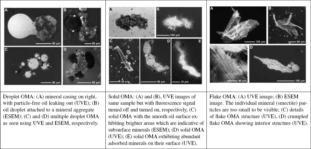
NOTE: Scale bars are shown in each image.
SOURCE: Adapted from Stoffyn-Egli and Lee (2002).
Mechanisms of Marine Oil Snow (MOS) Formation and Its Characteristics
Marine oil snow (MOS) forms when naturally or chemically dispersed oil droplets attach to marine snow and mineral particles (Brakstad et al., 2018c) (see Figure 5.29). MOS particles, defined as microhabitats <0.5 mm in size and rich in organic matter (Burd et al., 2020; Trudnowska, 2021), may form via two general mechanisms that are not mutually exclusive: (1) pre-formed aggregates interacting with oil, or (2) oil acting as a nucleus for microbial biofilm growth and floc formation (i.e., bacteria–oil aggregate or BOA) (Passow and Overton, 2021). Within these mechanisms are various processes and components that contribute to MOS formation including physical coagulation of marine particles, microbially mediated formation of marine snow, synthesis of biopolymers by algae and bacteria due to oil and dispersant exposure, and incorporation of oil into mucous feeding webs followed by ingestion of oil by zooplankton and/or attachment of oil to fecal pellets (MOSSFA, 2013). From the perspective of aggregation theory, oil droplets and marine particles collide and stick to form larger aggregates with the particle size and concentration determining the rate of particle collisions (Lambert and Variano, 2016).
The presence of non-biological particles such as suspended sediment from riverine sources or high-energy beaches, or black soot from in situ burning of surface oil also can contribute to MOS formation. Furthermore, application of chemical dispersants to oil slicks can stimulate EPS production and MOS formation (Passow, 2016). Dispersants allow oil to enter the water column as droplets by reducing the interfacial surface tension between the oil and seawater (see Section 5.3.1.2) so the presence of small but numerous oil droplets in water results in increased collision rates between droplets and marine particles and, therefore, increases the rate of MOS formation. However, experiments conducted with oil, diatoms, and the dispersant Corexit 9500A showed that Corexit inhibited the formation of MOS aggregates. Therefore, the net effect of Corexit 9500A on sedimentation rates of oil could not be quantified (Passow et al., 2017). Although the relative importance of dispersant, oil, and marine snow to the MOSSFA phenomenon observed during the DWH spill is difficult to ascertain in situ, controlled laboratory studies (Fu et al., 2014) noted that oil, Corexit EC9500A dispersant and suspended particulate matter, including living indigenous microbes, were all required to enhance MOS formation. Their hypothesis is that, when chemical dispersion increases the volume of small oil droplets in the water column compared with naturally or mechanically dispersed oil, the finely dispersed oil provides increased surface area and substrates for enhanced production of EPS and growth of microbial flocs, as well as facilitating physical interactions with natural suspended solids to form MOS having high oil content. Both sinking and rising of MOS were observed in the experiment (Fu et al., 2014); extrapolation to in situ conditions suggests that MOS sinking would generate a MOSSFA event. The importance of suspended matter in MOS production and growth suggests that deepwater oil plumes are less likely to generate MOS than surface waters. Note, however, that due to the inherent limitations of
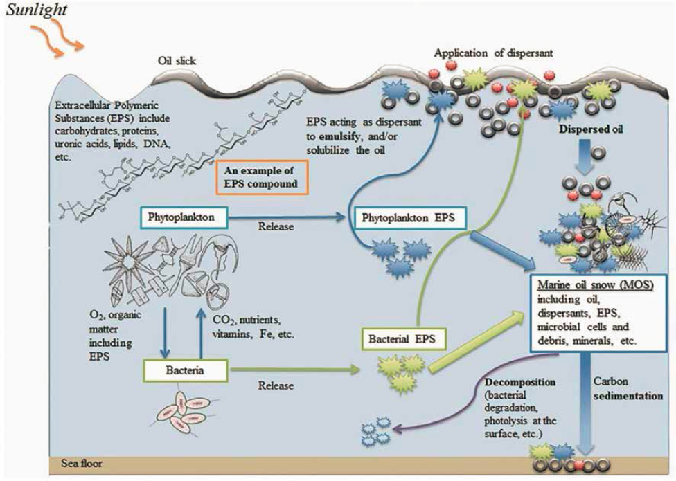
NOTES: EPS adsorbs and disperses oil, thus enhancing its solubility and bioavailability; provides a physical structure for microbes to assemble and degrade oil efficiently; and traps colloidal and particulate matter via coagulation, aggregation, and cross-linking processes. Thus, MOS aggregates may include EPS, oil, dispersant, cells or cellular debris, entrained solutes, particulates and other materials from the water column. Similar processes affect oil in the absence of dispersant when the oil is entrained by wind and waves into the surface water column.
SOURCE: Quigg et al. (2016). CC BY.
laboratory experiments, direct extrapolation to MOSSFA formation in the field may be challenging. The results should be viewed in the context of realistic concentrations, droplet size distributions, natural dilution rates, and other parameters relevant to field conditions.
Living organisms are a key component of MOS, affecting its formation and biochemical activity. Changes in the surface water microbial community composition that occur after oil spills (see Section 5.2.8.2) can affect the production of exopolymers and, subsequently, MOS formation and composition. Primary producers (phytoplankton) as well as heterotrophic bacteria that thrive in oiled water, such as strains of Alteromonas, produce large quantities of EPS that further enhance MOS formation, whereas strains of other hydrocarbon-degrading bacteria such as Pseudoalteromonas, and Cycloclasticus produce relatively small quantities of EPS (Gutierrez et al., 2018). Other biochemical activities also influence MOS characteristics: the patterns of polysaccharide- hydrolyzing enzyme activities in MOS differ significantly from the surrounding water matrix, and the enhanced lipase activity indicates increased biodegradation rates within the aggregates (Doyle et al., 2018; Kamalanathan et al., 2018). Oxygenation patterns in MOS extracts show degraded oil compounds similar to those of environmentally aged oil (Wozniak et al., 2019). That is, MOS aggregates include multifunctional microbial communities involved with oil biodegradation either directly as primary and secondary oil-degraders (e.g., by mineralizing, transforming, and/or assimilating hydrocarbons and degradation products), or indirectly (e.g., by emulsifying oil with EPS). In contrast to obligate hydrocarbon-degrading bacteria that specialize in biodegradation of petroleum components, most MOS species can utilize a broad range of substrates and do not depend exclusively on carbon sources originating from petroleum (Arnosti et al., 2016). Because the communities are dynamic, their composition can shift as the particles sink and oil components are biodegraded. Ultimately, the residual oil deposited with MOS on the seafloor is chemically different from the original spilled oil (Bagby et al., 2016), discussed in Section 5.3.3.6, and the diverse organic matter associated
with MOS can be further degraded in seafloor sediments, contributing to the benthic carbon cycle. Marine snow does not only occur in subtropical gyres but also has been reported in the continental shelf off North Carolina and in a fjord of the San Juan Islands (Washington), and in the Baltic Sea (Turner, 2015). Large accumulations of marine snow at a fjord in the San Juan Islands had discrete thin layers of diatoms. Photographs of dense marine snow accumulations in the Baltic Sea show copepods feeding upon particles of marine snow. There is ample evidence of the advances in the past two decades of in situ collection and visualization instrumentation that now facilitates documentation of the presence of marine snow/extracellular polymeric material as well as other particles accumulating on density gradients (Trudnowska et al., 2021). Dynamic interactions between the marine snow/extracellular polymeric organic material and other particles, feeding by some zooplankton, and microbial degradation of natural organic matter contribute to spatial and temporal variability of marine snow deposits.
Fundamental physical chemical properties of medium to higher molecular weight material predict adsorption/absorption to marine snow/extracellular polymeric organic material (see Chapter 2) and has been demonstrated in laboratory studies especially after DWH. It is important that future responses to oil spills, and consideration of the fate and effects of petroleum compounds from oil spills and other inputs, consider marine snow as a potentially important factor for fate of oil.
Environmental and Biological Controls on MOS Formation and MOSSFA Events
Formation of marine snow with incorporation of oil to generate MOS with subsequent settling to the seafloor (i.e., MOSSFA) is a mechanism proposed to explain the fate of some Macondo oil during and after the DWH spill (Quigg et al., 2020). However, it is difficult to quantify how much of the oil released during DWH was transported by MOS to sediments because some oil-containing flocculant material that settled was resuspended from the sediment–water interface and transported with underwater currents. Due to resuspension, sea floor sediment samples did not consistently detect oil but, conversely, oil-associated flocculant material indicative of MOS deposition was found in deep sea coral reefs during and after the DWH oil spill (Passow and Ziervogel, 2016).
Occurrences of MOSSFA events were reported in the literature at different geographical locations before the DWH spill (Quigg et al., 2020), although not by that acronym. However, pre-DWH literature mostly described shallow waters, near-shore environments (where there are high concentrations of mineral particles that promote formation of both MOS and OMA) and small-scale observations.
The phenomenon observed during DWH provided a new perspective for conditions that can result in a MOSSFA event due to (1) a very large quantity of oil entering the marine environment, (2) deep water (offshore) conditions, and (3) possibly the use of subsurface dispersants (Fu et al., 2014). Research efforts after DWH allowed better spatial and temporal resolution for observations and analyses of data to study the MOSSFA event (e.g., Romero et al., 2021).
Formation of MOS aggregates is affected by several combined factors including: timing and location of spill and of response measures, the state (i.e., degree of weathering) and chemical composition of oil, influences from the ocean and coastal environment (including interaction with riverine and shelf processes), and the type of marine biota present and their related processes (Daly et al., 2016; Gregson et al., 2021) (see Figure 5.30). Individually these conditions do not necessarily lead to significant oil deposition on the seafloor in MOSSFA events, such as that observed during the DWH oil spill (see Box 5.10). The deposition, accumulation and biogeochemical fate of oil and associated MOS on the seafloor are influenced by the dynamic interactions of benthic fauna (bioturbation, resuspension, feeding); presence of oil and dispersants (petrogenic hydrocarbons, smaller oil droplets, pyrogenic material generated from in situ burning processes); and riverine and terrestrial inputs of clays and organic matter (MOSSFA, 2013). For example, surface application of Corexit 9500A during the DWH spill was associated with unusually large in situ accumulations of MOS followed by MOSSFA events, described in Box 5.10 and Figure 5.29.
At present, the DWH oil spill is the most-studied example of MOSSFA contributing significantly to the fate of oil through sedimentation to the seafloor. Retrospective analyses suggest that MOSSFA events may have occurred during the 1979–1980 Ixtoc 1 spill in the Gulf of Mexico and other spills (Vonk et al., 2015; Schwing et al., 2020a), but currently it is unknown whether such large-scale events are common or significant outside the Gulf of Mexico and other temperate marine waters. The possible global significance of MOSSFA events should be examined so that, if relevant, they may be incorporated into response plans, oil spill budgets, and oil spill models, as needed.
5.3.2.3 Sorption to Plastics
Plastics are produced from petroleum hydrocarbons and enter marine environments; however, they are not considered in the same manner as oils (liquid or semiliquid) as their transport and fate are different from those associated with oil spills at sea. Plastics entering the marine environment and their fate are considered in a new study by NASEM (2021). Examples, as described by the Smithsonian Institution’s Ocean Portal Team,3 are provided in Box 5.11.
Plastics enter the marine environment through activities associated with fishing and aquaculture, intentional disposal
___________________
3 See https://ocean.si.edu/conservation/pollution/marine-plastics.
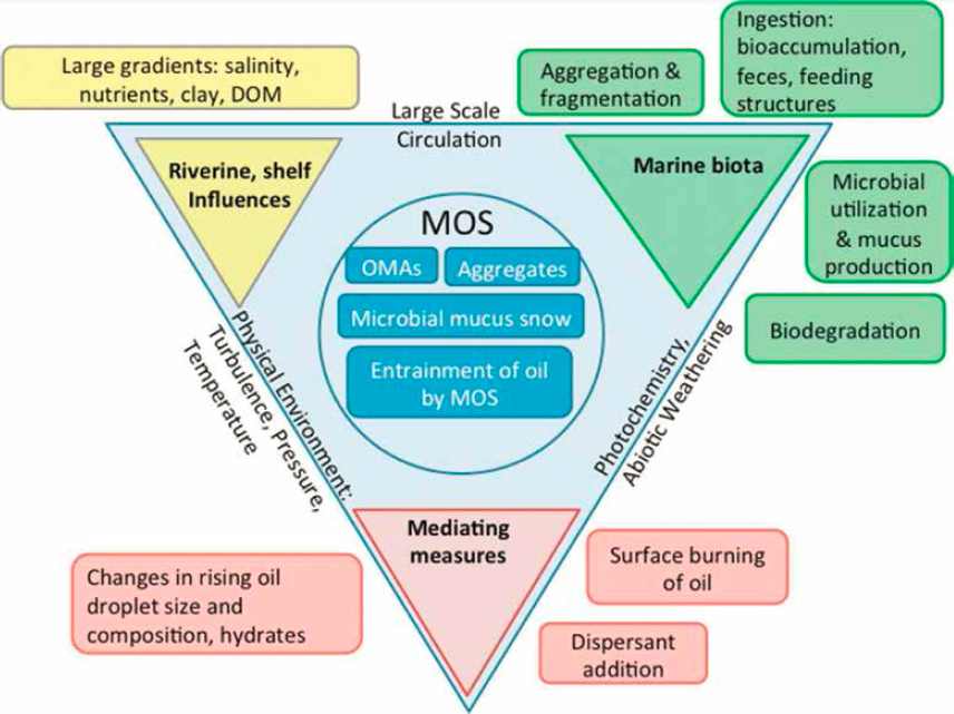
SOURCE: Daly et al. (2016). CC BY NC ND.
from vessels, and storm-related debris (Erickson et al., 2014; Hale et al., 2020). Plastics and construction debris are deployed in water bodies for the creation of artificial reefs to create habitats for finfish and shellfish. Episodic events such as storms and hurricanes in coastal areas result in floodwaters that carry significant quantities of plastics to coastal waters. Depending on the treatment processes used, wastewater discharges also may contain microplastics (MP). “Nurdles,” the preproduction building blocks for nearly all plastic goods, may enter the oceans through shipping mishaps. The pellets, weighing about 20 mg each, usually float or have neutral buoyancy. They absorb toxic chemicals from the water column and are often mistaken for food by animals.
Floating plastics in the marine environment are transported by wind, wave action, and ocean currents. Plastics can adsorb hydrophobic organic pollutants and metals, and the adsorption capacity increases with weathering and aging of the material (Yu et al., 2019; Li et al., 2020). Boom material used for oil absorption of oil spills is made of plastic compounds. As a result, once oiled, such booms may become another part of the plastics waste stream. Salinity, temperature, and pH can affect the adsorption characteristics of hydrophobic compounds on plastics. The petroleum-based hydrophobic compounds adsorbed on plastic debris also can be transformed and/or transported by photo-oxidation, biofouling of surfaces (microscopic, algae), marine growth (macroscopic), sinking/sedimentation, deposition on sediments, and consumption by marine organisms (e.g., fish, birds). It is estimated that atmospheric deposition of synthetic fibers (such as from laundering synthetic fleece) is between 3 and 10 metric tonnes each year, and on a 2,500 km2 area can deposit 355 particles m–2 day–1 with the majority consisting of small fibers 7–15 µm in diameter (Dris et al., 2016).
The circulation patterns in the oceans create accumulation zones on the ocean’s surface including plastic debris in subtropical gyres (Howell et al., 2012; Maximenko et al., 2018; Li et al., 2020). Physical oceanographic phenomena (e.g., Ekman transport, geostrophy) explain why plastic debris accumulates within the more calm areas of oceanic gyres, while more complex processes transport marine plastics in less obvious locales, including deep sea sediments and ice sheets (Hale et al., 2020).
Sedimentation rates and characteristics of microplastics are different from deposition characteristics of natural sediment. Microplastics have been found in deep-sea sediments cores from the Arctic Central Basin, North and South Atlantic, Southern Ocean, Mediterranean Sea, and Indian Ocean (Erni-Cassola et al., 2019; Kanhai et al., 2019). Microplastics are found in fish and other organisms, coastal sediments including beaches, shorelines (Browne et al., 2010), and coastal lagoons (Vianello et al., 2013). The most common polymers identified in the intertidal sediments from urban and semi-natural southwest Atlantic estuaries included polyethylene, polyethylene terephthalate/polyester, polyvinyl chloride, and polypropylene. Different microplastic characteristics among the estuarine environments suggests
TABLE 5.3 Fate and Transport Mechanisms of Plastics That Affect Fate and Transport of Oil in Marine Environments
| Sources of Plastics | Interactions of Plastics with Oil at Sea |
|---|---|
|
|
different anthropogenic sources (Díaz-Jaramillo et al., 2021). High concentrations of denser polymers (e.g., polyester, polyamide, and acrylic) are found in intertidal and subtidal sediments, as well as locations with periodic polystyrene inputs (Erni-Cassola et al., 2019).
At sea, these plastics can interact with oil and other hydrophobic compounds. Depending on the size of plastic particles and type of the polymer, different types of plastic particle–oil interactions can occur (see Table 5.3). Plastics can become covered by oil, microorganisms, algae, invertebrates, and other organic and inorganic materials that then secondarily are exposed to the oil. Biofilms on plastic debris may also support microorganisms that expel extracellular enzymes which may degrade oil and/or polymers (Dang and Lovell, 2016).
Oil adsorbed on macroplastics can be transported long distances with ocean currents. Microplastics can be incorporated into aggregates that form during coagulation of organic matter and oil droplets. Marine snow can transport microplastics of different shapes, sizes, and polymers and enhance their bioavailability to benthic organisms (Zhao et al., 2018). Mass sedimentation episodes of marine aggregates (e.g., MOS) can capture slowly sinking particles, including microplastics (Passow and Stout, 2020). Sinking rates of microplastics increased when incorporated into marine snow and also increased microplastic bioavailability for mussels (Porter et al., 2018).
Plastics are often ingested by marine organisms including micro- and nanoplankton species and oil adsorbed on the plastics can be metabolized (Andrady, 2011) (see Figure 5.31).
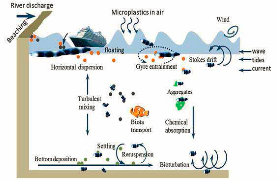
SOURCE: Modified from Li et al. (2020).
5.3.2.4 Submergence and Sinking of Heavy Oils and Semi-Solid Oils
Conventional oils are less dense than seawater and float or remain suspended in seawater even after weathering, whereas some unconventional oils have densities greater than that of freshwater (1.00 g/cm3) and therefore may sink in freshwater. Stated in terms of American Petroleum Institute (API) gravity, oils having >10° API will float and those of <10° API will sink in freshwater (NASEM, 2013). This behavior will differ in seawater, which has a typical density ≥1.02 g/cm3. Therefore, Bunker C (No. 6 Fuel Oil), ranging in density from 0.95 to ≥1.03 g/cm3 and with API gravity ~12° (see Chapter 2), may float or sink in seawater. Furthermore, interactions with mineral particles and/or organic aggregates as described in Section 5.3.2.1 may cause otherwise buoyant oil types to sink. For example, the inland Refugio pipeline spill in 2015 near Santa Barbara, California, released a diluted heavy crude oil that flowed over earth, sand, and gravel before entering the ocean. Much of the oil floated and oiled nearby beaches, but a portion submerged and sank, likely because it adhered organic and mineral particles from the beach and surf zone, and affected near-shore reefs and kelp beds (NASEM, 2016a).
Natural (undiluted) bitumen has a density of 0.977–1.016 g/cm3 and API gravity <10° (Fingas, 2015), in principle allowing it to sink in fresh or brackish water but not seawater. However, it is not transported (or spilled) as neat bitumen but rather as dilbit, a blend of bitumen and light hydrocarbon diluent (see Chapter 2). The diluent decreases the density of the blend sufficiently to enable spilled dilbit to float, at least initially, but floating results in rapid evaporation of a significant proportion of diluent, enabling the residual dilbit to sink in freshwater, as observed in laboratory studies (e.g., Stoyanovic et al., 2019) and in the Kalamazoo River spill in 2010 (NASEM, 2016a). The potential for sinking in seawater and brackish water has been debated and, in the fortunate absence of significant marine spills of dilbit, a variety of laboratory and ex situ tests using outdoor flumes and tanks has been conducted to gain insight into sinking potential under simulated spill conditions. The relevance of some observations has been criticized because some experiments failed to include one or more environmental factors such as solar irradiation (precluding photo-oxidation effects), in situ water temperatures (affecting oil viscosity and evaporation), relevant mixing energy (affecting dispersion of oil), oil confinement (slick thickness, affecting evaporation), and presence/absence of suspended sediments (OPA formation; see Section 5.3.2.1). Nonetheless, trends can be discerned from the combined results. In laboratory simulations, Hua et al. (2018) found that the weathering state of dilbit and the particle size and type were major factors influencing interaction and buoyancy in synthetic seawater. Sediment loads similar to seasonal maxima at coastal river outflows formed OPAs when mixed artificially with fresh or lightly weathered dilbit (0% or 16% mass loss) and subsequently sank, whereas heavily weathered dilbit (25% mass loss) had less interaction with sediment and formed submerged oil balls, some of which later resurfaced but did not sediment. Sand particles had almost no interaction with dilbit in comparison with clay and benthic sediment particles (Hua et al., 2018).
The general consensus appears to be that weathered dilbit can submerge (but not sink) as discrete oil balls in brackish water and even in sediment-free coastal seawater (King et al., 2014), especially in fjords or near river outfalls if heavy rainfall decreases the salinity of the upper 1–3 m of water (Johannessen et al., 2020). Light or mild weathering of dilbit could increase OPA formation, given sufficient sediment load and mixing energy, but would also maintain buoyancy so that lightly weathered dilbit should not sink in coastal seawater with seasonal densities of ≥1.02 g/cm3 (Ortmann et al., 2020) and therefore would not sink in higher salinity offshore seawater. Heavily weathered dilbit is more dense, but interacts less with suspended sediment and therefore is more likely to form suspended oil balls than to sink. The possible contribution of dilbit to MOSSFA events (see Section 5.3.2) has not been examined, but because weathered dilbit is poorly available, with only very selective biodegradation having been documented in situ (Schreiber et al., 2021), theoretically it should not support marine snow formation to enhance sedimentation. Although research into the fate of heavy oils and diluted bitumen in the ocean has accelerated in the past decade, some questions remain regarding weathering properties, behavior (particularly the sinking potential), and biodegradability of such oils in the sea; additional ex situ research under relevant conditions would help address this knowledge gap.
5.3.3 Deep Sea and Deep Sediment Processes
Accidental subsea releases of oil and gas include oil well blowouts, pipeline leaks, and releases from sunken ships. Near-surface processes (see Section 5.2.1) are mostly limited to the upper mixed-layer of the ocean. Here, we consider processes below 1,000 m depth, extending to the deep seabed. Leaks from accidental oil well blowouts or pipeline ruptures are expected to be localized, energetic inputs of oil, gas, or mixtures of oil and gas. The Ixtoc I and Deepwater Horizon oil well blowouts are historical examples. These may form an atomized spray of oil droplets and gas bubbles from the release orifice that combine with entrained seawater to form buoyant jets, which rise as buoyant plumes through the ocean water column, and depending on the depth, form lateral, subsurface intrusion layers (Socolofsky et al., 2011). Above an intrusion layer, individual bubbles or droplets may continue to rise by their own terminal rise velocity (Dissanayake et al., 2018). Alternatively, if the well failure causing an oil well blowout occurs subsurface, it is possible that oil and gas would flow into the sub-bottom geologic formation and percolate diffusely through the
seabed sediments. This may result in much less rigorous releases distributed over a larger area such that droplet and bubble formation follow different dynamics, and a buoyant plume stage of transport may not form. Similarly, releases from sunken ships would be expected to have much less energy at the source, forming oil droplets by sinuous-wave breakup (Masutani and Adams, 2000). Entrainment of ambient seawater and formation of a buoyant plume would not be expected. Like the bubbles or droplets escaping the intrusion layers of the more rigorous blowout plumes, droplets released from diffuse seabed leakage and sunken ships rise at their individual terminal velocities. Hence, the main differences among these types of subsea releases are in the droplet formation dynamics and whether or not a buoyant plume stage may be expected.
As noted earlier, most of the fate processes for oil in the sea depend on the interfacial area of the droplets or bubbles, which increases per unit volume of oil as the droplet size decreases. Smaller droplets also rise slower and are transported along different trajectories than larger droplets. One process that accelerates the vertical rise of droplets independent of their sizes is a buoyant jet or plume. When a plume forms, it can transport small oil droplets or gas bubbles at plume speeds of about 0.5 to 1.0 m/s (Gros et al., 2020). Eventually, oil and gas plumes transiting the ocean water column are arrested by the ambient density stratification and will form a lateral intrusion at a level of neutral buoyancy. Bubbles and droplets may rise out of this intrusion at their own terminal rise velocity, rising toward the surface without the assistance of subsequent plumes. Point-source releases from broken pipelines or a crippled oil well are expected to have a buoyant plume stage of transport. Releases from sunken ships or diffuse seepage over a wide region of the seabed leads to weak plume coherence; hence, the plume stage of transport would not be expected (Wang et al., 2019, 2020), and oil and gas would rise at their terminal velocity throughout their ascent from the source.
5.3.3.1 Plume Dynamics and Intrusion Formation
For an oil well blowout or pipeline leak through a localized orifice with sizes of order 1 m in diameter or smaller, the released oil and gas would be expected to mix with ambient seawater and form a buoyant jet at the release that would quickly transition to a vertically rising buoyant plume. The dynamics of this buoyant plume will depend on the total buoyancy flux of oil and gas released at the source, and droplets and bubbles engulfed within the plume would rise at the plume velocity plus their terminal rise velocity (Socolofsky and Adams, 2005; Dissanayake et al., 2018). To understand the breakup dynamics causing formation of oil droplets and gas bubbles, we need to consider the turbulent dynamics in the buoyant jet and plumes stages of transport. To predict the rise of these droplets and bubbles in the ocean water column, we must also understand the buoyant plume dynamics and its interactions with ambient ocean currents and density stratification.
There are three stages of turbulent dynamics moving from the release point to the buoyant plume. At the release, the turbulent properties may be characterized by the turbulence upstream of the release, normally some form of pipe-flow turbulence. Once released to the ocean, this stream of oil and gas rapidly mixes with seawater through a zone-of-flow-establishment (ZFE) to form a buoyant jet. When gas, which carries high buoyancy, is released the jet, which is dominated by the released momentum, quickly transitions to a plume, which is dominated by the released buoyancy. See Lee and Chu (2003) for a comprehensive review of these dynamics applied to single-phase (e.g., wastewater) discharges. For the DWH oil spill, the release at the end of the broken rise transitioned from the pipe flow to a buoyant plume (vertically rising) within one frame of the ROV camera, or a few pipe diameters downstream. Bubble and droplet breakup will follow different dynamics in the ZFE, jet, and plume stages of a blowout because the dissipation rate of turbulent kinetic energy follows different scaling laws within each of these regimes. Within the ZFE, the turbulent dissipation rate is constant and depends on the release velocity and orifice diameter. In the jet stage, the turbulent dissipation rate rapidly decreases, scaling with inverse distance from the source to the fourth power. The decrease in turbulent dissipation rate is less in the plume stage, scaling with inverse distance to the second power, owing to energy input from the buoyancy driving the plume. These scaling laws are likewise reviewed for single-phase releases in Lee and Chu (2003) and applied to breakup of oil droplets by Zhao et al. (2014).
In multi-phase flows, involving immiscible bubbles or droplets like releases of oil and gas into seawater, the behavior alters from that of single-phase plumes due to the slip velocity of the bubbles and droplets relative to the entrained seawater. Two main consequences are important here. First, bubbles and droplets are not required to follow the entrained seawater but instead may separate from the plume (see Figure 5.32). This may occur in lateral currents that bend over the plume in the downstream direction (see Figure 5.32a)—the vertical rise velocity of the bubbles or droplets then causes their trajectories to escape on the upstream edge of the entrained seawater plume (Socolofsky and Adams, 2002; Murphy et al., 2016). This may also occur when ocean density stratification prevents the entrained seawater from rising above a level of neutral buoyancy (see Figure 5.32b), where the entrained seawater plume would be expected to be arrested by the stratification and intrude laterally (Socolofsky and Adams, 2003, 2005). In the deep oceans, both currents and density stratification may be important. Figure 5.32c depicts the case of a stratification-dominated plume in a weak crossflow; separation dynamics and empirical equations for predicting the occurrence and scales are discussed in more detail in Socolofsky et al. (2011).
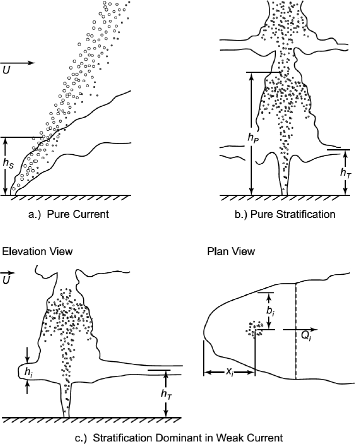
SOURCE: Adapted from Socolofsky et al. (2011).
Second, the presence of bubbles or droplets in the flow breaks down the assumptions used to derive solutions for single-phase buoyant; namely, self-similarity is no longer strictly valid (Socolofsky et al., 2008). This means that turbulence dynamics in the flow are altered somewhat from their single-phase analogues. Plume spreading may be affected by the breakdown in self similarity (Seol et al., 2009), and the classical entrainment coefficient is no longer constant along the plume trajectory (Milgram, 1983; Seol et al., 2007). This is important for the development of one-dimensional integral models based on the entrainment hypothesis; however, as for single-phase plumes in density stratification, models based on self-similarity remain robust even for significant deviations from the self-similarity requirements (Turner, 1986). An important consequence of this fact for understanding oil well blowouts is that the turbulent eddy dissipation rate may not follow correlations for classical jets and plumes, with important contributions to the turbulence production term arising from the wakes of the oil droplets and gas bubbles (Fraga et al., 2016; Zhao et al., 2016, 2017; Lai et al., 2019).
For more details on the plume dynamics as they relate to accidental oil well blowouts, see the reviews by Socolofsky et al. (2016) and by Boufadel et al. (2020a,b).
5.3.3.2 Bubble and Droplet Breakup from Subsurface Leaks
Since the 2003 Oil in the Sea report and following the DWH oil spill, there has been tremendous advancement in data and models to predict the droplet and bubble sizes of oil and gas released subsea. Here, we consider both slow or diffuse releases as well as oil well blowouts. Oil droplet size is important in subsea releases because it determines the rise velocity of the droplets and sets the interfacial area
for dissolution and biodegradation fate processes. For deep releases, these fate processes may represent a significant fraction of the overall release mass balance.
Oil droplet formation for subsea releases may occur by different mechanisms, depending on the flow rate and source geometry. Masutani and Adams (2000) reported on these breakup processes based on observations of different types of oil into water. They showed that at slow releases, droplet breakup is by pendent drop formation at the lowest release rates followed by sinuous wave breakup as the release rate increases. At higher flow rates, an atomization breakup regime is found. The boundary defining the onset of atomization occurs at a jet Weber number of 324 (Johansen et al., 2013). Droplet sizes for the pendent drop formation and sinuous wave breakup scale with the smaller of the orifice diameter or the maximum stable droplet size for a drop rising in a quiescent ambient fluid (Clift et al., 1978). Droplet sizes in the atomization stage depend on the turbulence dynamics at the release and in the ensuing jet or plume. Slow or diffused subsurface releases fall outside the atomization region; accidental oil well blowouts likely fall in the atomization region.
Slow or Diffused Subsurface Releases
For oil releases from sunken wrecks, natural seeps, or diffuse seepage through the seabed from a subsurface oil well blowout, the droplet formation process follows the pendent drop or sinuous wave breakup modes. For a wide range of oils, the maximum stable droplet size is about 10 mm in diameter (Li et al., 2017). Maximum stable gas bubbles sizes are more complicated to estimate, requiring an iterative solution to a stability analysis problem (Grace et al., 1978). For typical natural gases in seawater, maximum stable bubble sizes can be over 100 mm in equivalent spherical diameter. Hence, bubble sizes scale more often with the orifice diameter. For example, for a wide range of natural gas seeps in the deep Gulf of Mexico and for laboratory experiments using air in a 16 m deep tank, gas bubble size distributions ranged from 1 to 10 mm, with median diameters of about 5 mm and maximum sizes up to 15 mm (Wang et al., 2016, 2018, 2019, 2020). These sizes are similar to the expected oil droplet size from weak sources, assuming no chemical dispersants are used, which is reasonable for these slow or distributed sources. As a result, for diffuse or weak sources, millimeter-scale droplets and bubbles are expected to form via non-atomizing breakup processes.
Strong Buoyant Jet Releases
For releases from broken pipelines or accidental oil well blowouts, the droplet formation process is expected to follow dynamics in the atomization regime of breakup. There, the turbulence in the released fluids and entrained seawater act to achieve breakup, with breakup following the Weber number and viscosity number parameterizations given by Hinze (1955) and Wang and Calabrese et al. (1986) (see Section 5.2.2.3 and Box 5.3). To apply these scaling relationships in empirical equations for droplet size, the dissipation rate of the turbulent kinetic energy must be evaluated for the buoyant jet dynamics in the primary breakup regime of the release. As noted above, strong buoyant jet releases include a ZFE, jet, and plume stage of development, and different scaling relationships for turbulent dissipation rate apply within each of these zones. Approaches using empirical equations normally take the turbulence characteristics from relations valid within the ZFE (Johansen et al., 2013; Li et al., 2017; Brandvik et al., 2021). Population balance models, which can consider time-varying turbulence properties, may consider all three stages from the ZFE to the plume transport stage (Zhao et al., 2014; Nissanka and Yapa, 2016). Appendix F includes a brief summary of how these approaches arrive at their model equations. Whichever approach is used, the equations and models must be calibrated and validated to measured droplet size distributions for experiments involving localized releases into water.
When conducting laboratory experiments in fluid dynamics, it is normally required to identify the governing non-dimensional variables, here the Weber number and one of either the viscosity, Reynolds, or Ohnesorge numbers (see Box 5.3), and to match their values between the laboratory experiments and the field-scale prototype. This approach is called dynamic similitude. For oil jets into water using crude or refined petroleum products as the dispersed phase, it is not possible to match the Weber and viscosity numbers between the laboratory and the field without conducting the laboratory experiment at full scale or changing the scales of the jet to plume transition. As a result, existing observations must be extrapolated to the field scale.
Figure 5.33 shows an example of the laboratory and field data available during the Model Intercomparison Study reported by Socolofsky et al. (2015), extended with data at higher modified Weber number from Brandvik et al. (2021). The data are plotted using the modified Weber number, defined by Brandvik et al. (2013), which combines the Weber and viscosity numbers into a single parameter. Symbols show the laboratory and DeepSpill field observations. The parameter space of the DWH oil spill is also shown as the shaded region in the figure along with extrapolated predictions for the droplet size of untreated DWH oil using the empirical equations of Johansen et al. (2013) and Li et al. (2017) and the population balance prediction of Gros et al. (2017). These model predictions for the DWH span more than an order of magnitude in the non-dimensional droplet size: clearly, extrapolating the observations to the scale of the DWH is difficult. One solution might be to use different fluids with properties yielding the field-scale parameters, but to have an accurate physical effect of the potential subsea dispersant injection, real oils and dispersants must be used in the experiments. This difficulty in making relevant laboratory measurements at adequate scales has been noted
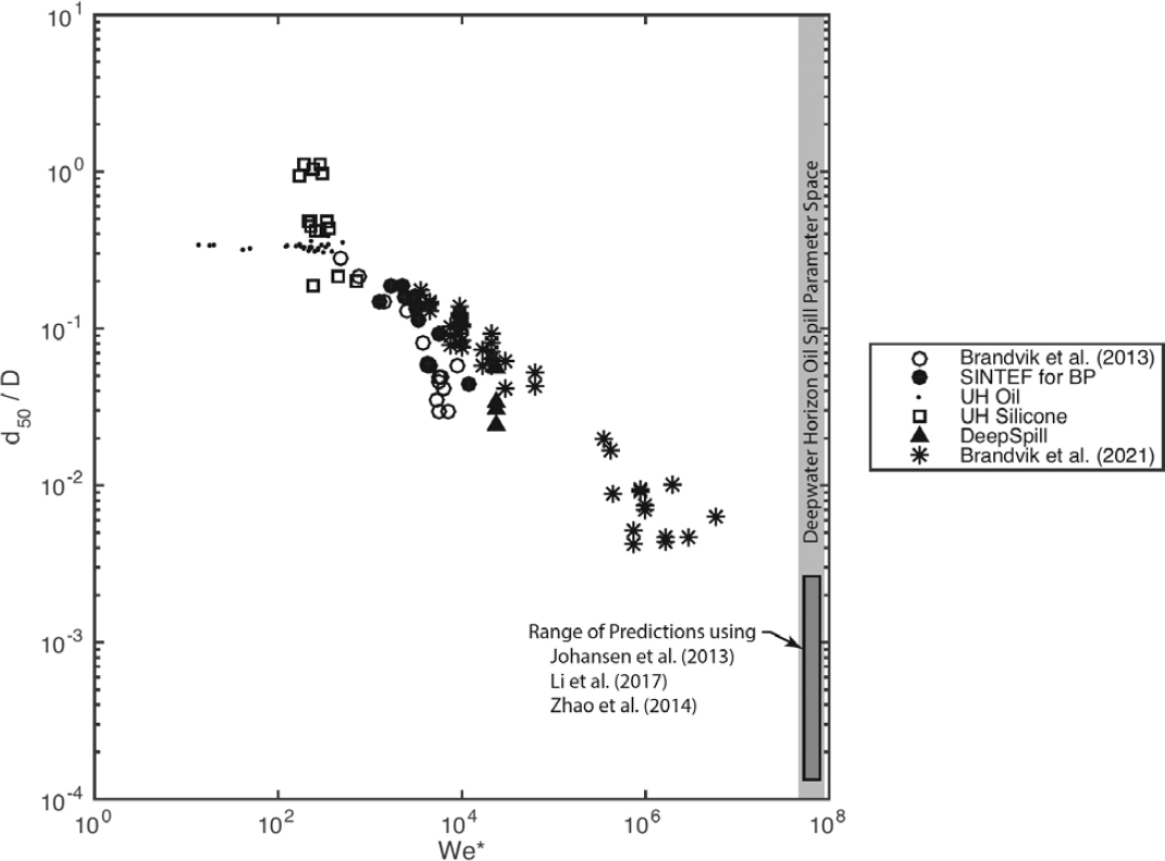
NOTES: Laboratory data include data published in Brandvik et al. (2013) using the SINTEF Tower Basin, additional data collected by SINTEF in the Tower Basin and provided to British Petroleum, data reported in Masutani and Adams (2000) for experiments at the University of Hawaii for crude oil and silicone oil, and data reported by Brandvik et al. (2021) for experiments in the Ohmsett facility. The results of the DeepSpill field experiment (Johansen et al., 2003) are also shown. The grey region on the right-hand-side of the figure depicts the parameter space relevant to the DWH using flow rate and property data reported by Gros et al. (2017) for June 8, 2010. The highlighted gray bar spans the range of droplet size predictions obtained using the empirical equations from Johansen et al. (2013) and Li et al. (2017) and the VDROP-J model (Zhao et al., 2014), each computed using the flow and property values reported by Gros et al. (2010) for June 8, 2010. Note that the field-scale parameter space is at nearly two orders of magnitude higher in the modified Weber number than the data; hence, extrapolation is required to make predictions. Moreover, the model predictions span a full order of magnitude. The smallest droplets are predicted by the Li et al. (2017) model; the largest droplets are predicted by VDROP-J (Zhao et al., 2014); and the Johansen et al. (2013) predictions using the update parameter calibration falls near the middle of the plotted span of data. Whether laboratory trends may be extrapolated linearly in log-log space to make the field-scale predictions requires additional data for validation.
SOURCE: Brandvik et al. (2013).
numerous times previously (NASEM, 2020) and remains a problem for validation of droplet size equations and models today. Because complete dynamic similitude is not achieved between existing jet break-up experiments and field prototypes, large-scale field or laboratory experiments are needed to demonstrate the reliability of existing droplet-size prediction equations to the field scale. This can be achieved either by full-scale experiments or by demonstrating the prediction results at smaller scales become independent of the non-matched scaling parameters. These data are needed for oil droplet breakup with and without co-flowing gas and with and without subsea dispersant injection.
One approach to bridge this gap is to utilize physics-resolving numerical models. Aiyer et al. (2019) developed a numerical approach that combines the population balance equations within a large eddy simulation (LES) fluid dynamics model to solve for the evolution of the droplet size distribution in space and time owing to the resolved and subgrid scale turbulent energy predicted by the LES. The population balance model follows the approach of Zhao et al. (2014a), but includes breakup within the viscous subrange; the LES
treats the dispersed phase using an Eulerian description (Yang et al., 2015). Aiyer and Meneveau (2020) adapted the coupled population balance and LES model to an oil jet into water, using a one-dimensional approximation of the model at the orifice to resolve the smallest scales of jet and breakup dynamics. This approach allows the ability to study the nonuniform and unsteady breakup dynamics. Importantly, they were able to quantify the evolution of characteristic diameters of the distribution, including the total surface area of the whole size distribution, given by the Sauter mean diameter of the simulated distribution. Although the actual size distributions showed strong dependence on the Weber number, the shapes of the lateral profiles of normalized properties of the size distribution did not depend on the Weber number. This indicates that the breakup process is largely self-similar and that the approach in VDROP-J, which uses uniform distributions of velocity and size distribution, is appropriate.
Other scaled experimental observations also study details of the breakup physics, including the effects of pressure, live oil, and the fine-scale details of droplet formation and turbulence in the immediate vicinity of an oil jet release. Malone et al. (2018) released dead and live oil mixtures of Louisiana sweet crude (LSC) and n-decane, using methane as the gaseous chemical species for creating the live oil liquids in the live oil experiments. They simulated the breakup of droplets from a circular orifice and measured the size distributions. For both LSC and n-decane, the measured droplet size distributions had larger median droplet sizes for the live oil cases than for the dead oils by about a factor of 2 despite the live oils having lower viscosities and only slightly higher interfacial tensions to the corresponding dead oils (Malone et al., 2018). Aman et al. (2015) also used live oil in high-pressure experiments for a mixing tank (i.e., not a jet into water). Although they did not observe dead oil, droplet sizes observed for the live oil experimental conditions agreed with predictions based on empirical models fit to literature data on water-in-oil mixing systems at atmospheric pressure. This suggests that the breakup of live oils can be predicted using equations fit to data for dead oils, provided the live oil properties are used with the prediction equations. Indeed, experiments reported by Brandvik et al. (2019) for live oil and gas jets into water at high pressure showed good agreement between predictions using the Johansen et al. (2013) equation with in situ live-oil properties. They found no effect of pressure. The effect of co-released gas was to reduce the oil droplet sizes compared to experiments with the same pure oil flow rate owing to the higher exit velocity of oil when released with gas. A mild effect of pressure in oil and gas releases was also observed due to the increased density of gas with higher pressure, resulting in greater momentum flux at the release. In summary, it appears that droplet size distribution models developed using experiments for dead oil at atmospheric conditions accurately capture the relevant physics and may be used for live oil at high pressure provided the relevant release dynamics, including in situ buoyancy, momentum fluxes, and oil and gas properties, are evaluated.
Laboratory experiments utilizing measurements at the droplet scale of droplet formation from a jet were reported by Xue and Katz (2019). They used a silicone oil jet into sugar water in order to match the index of refraction in the dispersed oil and continuous water phases; they visualized the breakup process immediately above the nozzle and to distances of 30 nozzle diameters using planar laser induced fluorescence (PLIF). Sample results for three different jet Reynolds numbers are shown in Figure 5.34. The experimental images clearly show the engulfment of ambient water by entrainment into the oil phase and the later breakup of the oil into droplets. A distinguishing feature of the formed droplets was the inclusion of smaller water droplets within individual oil droplets for the experiments with jet Reynolds numbers of 1358 and 2122. These compound droplets had been observed in previous droplet breakup studies, but not previously for jet breakup. The included water increases the bulk density of the oil–water mixture of a compound droplet compared to the density of pure oil. The included water also increases the total surface area of oil exposed to seawater. For some of the larger oil droplets, multiple water droplets were included, sometimes as a cascade of Russian dolls, with water inside oil inside water inside oil. The droplet breakup process was observed to continue to at least 30 nozzle diameters downstream, indicating that primary breakup occurs beyond the ZFE of the buoyant jet and out into the self-similar region of these multiphase plumes.
Similar fine-scale experiments were also reported by Xue et al. (2021), including also velocity measurements of the oil and water phases separately using high-resolution particle image velocimetry (PIV) simultaneously with PLIF. The final spacing between PIV velocity vectors was as small as 128.5 µm. From these data, Xue et al. (2021) could compute the time-average velocity and fluctuating statistics in both the oil and water phases, as well as the turbulent kinetic energy production. They found higher turbulence levels than in a single-phase jet, though this difference decreased with distance from the nozzle. They also found differences between the turbulence magnitude and characteristics for the oil-phase and water-phase turbulent fluctuations. The water had higher turbulent kinetic energy than the oil near the nozzle. At distances greater than six nozzle diameters from the release, the turbulent kinetic energy is higher in the oil than the water. These effects demonstrate the transfer of energy from the oil to the water via entrainment near the source and the subsequent production of turbulent kinetic energy in the oil by the water downstream of the jet orifice. Turbulent kinetic energy production is higher in the oil along the edges of the jet, and higher in the water along the jet centerline, both effects owing to the different mechanisms of turbulence production in the oil and water. These data will be important to further validate numerical models of oil jets into water and to evaluate the assumptions and turbulent quantities used
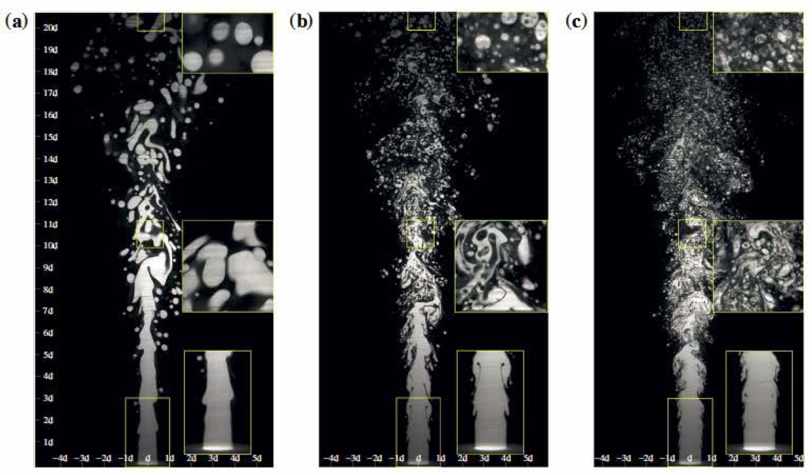
NOTES: Jet Reynolds numbers are (a) 594, (b) 1358, and (c) 2122. Insets on the right-hand side of each image correspond to the smaller, highlighted region in the main jet. These images show the entrainment of ambient water (black) into the oil jet (gray-scale), creating filaments and blobs of oil and subsequently break up into individual droplets. The insets show the details of the formed oil droplets, which include many compound droplets composed of water droplets suspended in oil droplets and sometimes cascading as in a set of Russian dolls. These data help to elucidate the mechanisms of droplet breakup and the structure of the formed droplets for different release conditions.
SOURCE: Xue and Katz (2019).
by equations and models to predict droplet breakup. High resolution imaging and data collection technologies are providing better insight for advancing our understanding of subsea oil release phenomena to develop and refine appropriate mathematical models.
5.3.3.3 Formation of Natural Gas Hydrates
Natural gas hydrates are crystalline structures of water and gas molecules that are thermodynamically stable at the high pressure and low temperature of the deep oceans (Sloan and Koh, 2008)—at depths of order 100 m or more, depending on the gas composition and temperature profile. Hydrates can cause problems in petroleum production by blocking pipelines and seizing equipment. During response to deepwater oil spills, hydrates may interfere with response equipment or form shells on released gas bubbles. Hydrate shells on bubbles may change their mass transfer coefficients.
In the laboratory, gas hydrates are observed to form at the interface of gas and water after the ambient water phase becomes saturated with dissolved gas relative to the hydrate solubility limit (Warzinski et al., 2014b). Anderson et al. (2012) used this criterion to assess the conditions within an accidental oil well blowout plume under which hydrates may be expected to form. Due to higher temperatures in the deep oil reservoir and the expected rapid rise time from the reservoir to the leak orifice, the released oil and gas are expected to be very warm. For example, temperatures measured during DWH were as high as 105°C (Reddy et al., 2012). Anderson et al. (2012) used an integral model to predict the evolving temperature and dissolved gas concentration in the plume resulting from oil and gas dissolution and entrainment of cold, ambient water. They concluded that by the time the plume cooled to a temperature favorable for hydrate formation, the dissolved gas concentration was diluted by entrained water adequately that hydrates were unlikely to form for the typical blowout cases simulated.
This is not to say that hydrates play no role in accidental subsea oil well blowouts. On the contrary, they were a major factor complicating the response to the DWH accident. As Anderson et al. (2012) also point out, hydrates do form rapidly wherever water and released gas collect, as under and
within subsea and response equipment. A good example is the failure of the coffer dam intervention during DWH, which rapidly became clogged with hydrates (McNutt et al., 2011). Hence, the top hat device used to eventually shut in the DWH leak was carefully engineered to avoid hydrate clogging. Hydrate formation has also been studied for natural gas releases from seafloor seeps; this is discussed in conjunction with dissolution in Section 5.3.3.4.
5.3.3.4 Gas Ebullition and Dissolution
Oil and gas released subsea, whether from an oil well blowout, pipeline leak, or diffuse seepage through the seafloor, is expected to enter the ocean water column as live petroleum droplets and bubbles. The soluble components within these fluid particles will immediately begin to dissolve and, depending on their initial conditions and rise speed, may experience phase changes. Gas bubbles may evolve out of the liquid petroleum phase via ebullition; gas bubbles may condense to liquids after dissolution of their lighter components. Whether these phase changes occur depends on the kinetics of dissolution and ebullition, the degree of initial supersaturation of gases in the liquid phase petroleum, the evolving mixture composition, local thermodynamic state, and the rise rate of droplets and bubbles.
For an accidental discharge directly from a crippled wellhead or pipeline leak, supersaturation of gas in the liquid phase may occur. As reservoir fluid is transported through the subsurface pipeline to the leak point, the pressure will be decreasing, and gas will be evolving out of the liquid phase. If the ebullition kinetics are not fast enough for the gas–liquid petroleum system to be at equilibrium with the temperature and pressure at the release, the liquid petroleum would be super-saturated with gas, in equilibrium with a higher, down-hole pressure and temperature. Observations of the in situ fluid phase equilibrium at a full-scale release of live petroleum fluids has not been made; hence, conclusions that may be drawn are tentative, based on limited laboratory observation and modeling.
For shallow releases, significant amounts of free gas may survive to the sea surface. When the gas arrives at sufficient atmospheric concentration, the gas may ignite and burn. This was the case for the gas released in the Ixtoc I blowout and for a recent gas pipeline leak in the Gulf of Mexico. Figure 5.35 shows a photo of the burning gas for that pipeline leak as it exited the water column near an offshore platform. Hence, predicting the fire hazard of gas released subsea requires accurate estimation of both the subsea gas plume dynamics and gas dissolution. If the majority of gas is dissolved subsea and is sequestered in a subsea intrusion layer, surface exposure or fire risk is low, as was the case for the DWH oil spill. When free or dissolved gas does reach the atmosphere in sufficient volumes, explosion and fire hazards are expected.
In oil and gas releases, the gas components must be tracked in both the gas and liquid phases of the petroleum. In a high-pressure water tunnel, Pesch et al. (2018) studied single, live-oil droplets under simulated deep-ocean conditions. They observed the droplet size evolution and considered

SOURCES: NOAA ORR, https://upload.wikimedia.org/wikipedia/commons/a/a6/IXTOC_I_oil_well_blowout.jpg.
cases with depressurization corresponding to high rise speeds, as may be experienced in an energetic plume of oil, gas, and entrained seawater, and slower rise speeds, closer to the rise rate of the observed droplets. Droplets remained of similar size over the majority of their depressurization, growing significantly in the final few tens of meters of simulated rise. Dissolution of methane from the droplet into the recirculating water was evident by gas bubbles that formed in the water below on the side-walls of the apparatus at system pressures below 5 bar.
Gros et al. (2020) applied the TAMOC model to simulate the dissolution and ebullition dynamics of the Pesch et al. (2018) experimental dataset. Gros et al. (2020) used the same model set up as for their hindcast of June 8, 2010, of the DWH and reported in Gros et al. (2017). In those simulations, phase equilibrium and dissolution are modeled simultaneously for each gas bubble and oil droplet. For the Pesch et al. (2018) data, only oil droplets were considered. If free gas is predicted to exist in equilibrium with the petroleum mixture at any stage of the experiment, the TAMOC model immediately creates an attached gas bubble—ebullition kinetics were, thus, ignored, and degassing was assumed instantaneous. Over the stage of the experiments where the droplet sizes remained steady, TAMOC predicted dissolution kinetics to be faster than degassing. That is, supersaturation was not observed due to the rapid dissolution of methane into the circulating water. Only in the final 5 bar of depressurization of the simulations did gas appear, and this occurred largely due to saturation of dissolved methane in the recirculation water, preventing further dissolution of methane from the oil droplet. Corresponding theoretical simulations in an open ocean with background methane concentration showed that degassing is a negligible process for oil droplets over a wide range of initial conditions for all but potentially the final few meters of rise through the ocean water column (Gros et al., 2020).
To understand the role of hydrate formation on dissolution from individual gas bubbles, Warzinski et al. (2014a) conducted experiments for suspended gas bubbles in a high-pressure water tunnel (HPWT) at the U.S. National Energy Technology Laboratory. The full suite of experiments is reported in Warzinski et al. (2014) and Levine et al. (2015). They used high-resolution and high-speed video imagery to identify hydrates. They observed that gas bubbles in the millimeter diameter size range initially formed thin hydrate shells, and that these shells became thicker and more rigid as hydrates are more thermodynamically favorable (i.e., at higher pressures and lower temperatures). The effect of the hydrate skins was observable in the high-speed imagery in which the wave oscillations on the bubble–water interface were damped and then frozen by the hydrate formation. As in previous laboratory experiments (e.g., Masutani and Adams, 2000), hydrates did not form in the HPWT until the background gas concentration reached saturation of the liquid–hydrate system. Once hydrate formed, it remained stable even for different dissolved gas concentrations as long as the hydrate was thermodynamically stable. Because the background gas concentration was high in their experiments and the experiment durations were relatively short, bubble shrinkage rates owing to dissolution processes could not be accurately quantified. Nonetheless, these experiments demonstrate the key phenomenology of hydrate effects of natural gas bubbles.
Wang et al. (2016, 2020) utilized a similar approach to Warzinski et al. (2014a) to observe natural gas hydrates on bubbles released from natural seeps in the deep Gulf of Mexico. They developed a high-speed, stereoscopic video system (Wang et al., 2015), which they integrated with a remotely operated vehicle (ROV) to observe bubble size distributions and hydrate effects. The high-speed imagery confirmed that hydrate shells were forming on the bubbles based on the immobilization of the bubble–water interface after formation, which generally occurred within the first few meters of rise from the seabed. Parallel measurements included analysis of the gas composition from the source and quantification of the dissolved gases in samples collected within the gas bubble column. Although dissolved gas concentrations in the bubble stream were low compared to hydrate solubility, hydrates rapidly formed. This may have been due to nucleation of the hydrate formation from solid hydrate present in the marine sediments, but no definitive mechanism for the rapid hydrate formation at low ambient dissolved gas concentration was determined.
Wang et al. (2020) observed the rise heights of bubbles from natural seeps using acoustic multibeam sonar, mounted both on the hull of the research vessel and on the ROV. They simulated the gas bubble evolution using the measured bubble size distributions at the sea floor using TAMOC and applied acoustic models to convert the simulated bubble properties to acoustic backscatter. By comparing the modeled acoustic behavior to the measured multibeam data, they could validate the model predictions for gas bubble dissolution. As explained in Section 5.2.2, they found that initially, gas bubbles dissolve at rates predicted by clean-bubble mass transfer coefficients. This was also corroborated by analysis of the isotopic signature of the dissolved gas samples (Leonte et al., 2018). After hydrate formation, the mass transfer switches to rates given by dirty bubble mass transfer coefficients. The hydrate formation time was predicted by an empirical equation using the hydrate subcooling and the initial surface area of the bubble and calibrated to data in Rehder et al. (2009). Dirty bubble mass transfer rates were appropriate due to the immobilization of the bubble–water interface by the hydrate. Wang et al. (2020) also found that it was the free gas inside the bubble and not the hydrate shell itself that was most responsible for the bubble shrinkage. This is consistent with the observation that hydrate skins crack and mend as bubbles expand due to the decrease in pressure with height (Warzinski et al., 2014b).
Gros et al. (2017) likewise simulated the effects of hydrate shells for a hindcast of June 8, 2010, of the DWH oil spill using dirty bubble mass transfer rates and dissolution kinetics given by the free gas solubility rather than that of hydrate. Gros et al. (2017) applied dirty bubble mass transfer coefficients directly from the release due to the fact that chemical surfactants were being applied subsea on June 8. For simulations assuming no surfactant injection, it was assumed that oil released with the gas would act as a contaminant, leading to dirty bubble mass transfer coefficients. The good performance of the Gros et al. (2017) model compared to the measured data (see Section 5.2.3.4) supports the conclusion that hydrate dynamics within accidental subsea blowout plumes may be modeled using dirty bubble mass transfer coefficients and dissolution related to the free gas and oil solubilities at the bubble- or droplet-water interface; hence, providing guidance for simulating potential future, deepwater oil spills.
5.3.3.5 Effects of Subsea Dispersant Injection
Like surface application of chemical dispersants, dispersants may be used subsea to affect the formation of oil droplets (NASEM, 2020). As explained in Chapter 4, this method is normally applied locally, near the release source, and is referred to as subsea dispersant injection (SSDI). The effect of SSDI is to reduce the interfacial tension between the treated liquid petroleum and seawater (Socolofsky et al., 2015). The amount of interfacial tension reduction depends on the properties of the released oil, the amount of injected dispersant, and the mixing between dispersant and oil. Depending on the oil and injection methods, interfacial tension reduction factors could span from 300 times (Brandvik et al., 2013, for Oseberg blend in the laboratory) to 5.4 times (Gros et al., 2017, for DWH oil under field conditions). Brandvik et al. (2013, 2018) tested different injection methods. The consensus to date is that dispersant injection near the release orifice is the most effective, achieving the greatest reduction in interfacial tension for a given dispersant volume. Hence, most SSDI contingency plans call for application by a dispersant wand at the end of a supply line and maneuvered into the released fluids by an ROV.
By reducing the interfacial tension of the released oil, smaller droplets may be generated. As explained in Section 5.2.2, turbulence in the seawater acts to break up droplets, and oil interfacial tension and viscosity resist droplet breakup. By reducing the interfacial tension, smaller droplets may form. This is especially true for SSDI when the dispersant is injected upstream of the high turbulence region of the release. For example, most of the oil droplet breakup occurs within 50 to 100 times the release diameter for a blowout or pipeline leak (Zhao et al., 2015). By treating the oil directly at the release, smaller droplets may be expected to form in this primary breakup region (Zhao et al., 2014, 2015). At some point, further reduction in interfacial tension no longer results in smaller droplets as the oil viscosity will dominate the breakup resistance, and viscosity is not affected by chemical dispersants. This was especially evident through experiments conducted on simulated SSDI for oil jets under diverse conditions in the laboratory (Brandvik et al., 2015). Hence, for each crude oil and spill release scenario, there may be a different optimal dispersant injection that will minimize the droplet size, though this dispersant to oil ratio is expected to be on the order of 1:100.
Droplets treated by dispersant through SSDI may further undergo breakup as they traverse the ocean water column. This secondary breakup results from a process called tip streaming. See Section 5.2.1.1. Depending on the amount of dispersant contained in a droplet and its rise time, a significant amount of oil may leave the droplet through this process, resulting in a dispersion of many, micron-sized droplets (Gopalan and Katz, 2010; Davies et al., 2019). As a result, SSDI affects droplet sizes by both reducing the average interfacial tension throughout the primary breakup zone near the source and by allowing some droplets to continue to break up into a chain of micron-size droplets through the process of tip streaming.
As has been carefully discussed in this chapter, the fate and effects of an oil droplet in the ocean are critically dependent on its size. This is the case because droplet size determines the available surface area for exchange (both for dissolution and biodegradation); sets the rise velocity, hence the residence time, of a droplet in the ocean water column; and dictates the trajectory of droplets rising through unsteady, non-uniform ocean currents. These processes critically determine the effects of the spilled oil in the ocean (see Chapter 6). Hence, if SSDI alters the droplet size, it will change the fate and effect of the spilled oil.
For example, by reducing the droplet size, SSDI acts to increase the total amount of dissolved hydrocarbons entering the deep sea, thereby reducing the amount of volatile compounds reaching the sea surface and the atmosphere (Gros et al., 2017; Zhao et al., 2021). When used effectively, SSDI may also result in droplets that spread out over wider areas, resulting in thinner sheens and slicks than for untreated releases. Gros et al. (2017) considered the effectiveness of SSDI during the DWH oil spill using a numerical simulation for June 8, 2010, a period for which intensive observations were available and SSDI was conducted at the end of the severed well head. Because of limitations in dispersant availability and application tools, the dispersant to oil ratio was not optimal on June 8, achieving an average dispersant to oil ratio of 1:250 and interfacial tension reduction estimated to be 5.4-fold. This resulted in oil droplets that were simulated to be 3.2-fold smaller than untreated droplets, though still having a volume median diameter of 1.3 mm. Because the droplets remained in the millimeter size range with SSDI application, the location of the surfacing oil and the total mass flux of liquid oil reaching the sea surface was minimally affected. However, this modest reduction in droplet size
significantly affected the dissolution of the light, soluble volatiles. For example, benzene mass fluxes to the atmosphere were reduced by over 2,000 times with this SSDI operation compared to simulations without SSDI. This resulted in significantly improved air quality within the response zone. This has recently been corroborated by an analysis of VOC alarm data for the entire DWH incident, which showed significantly improved air quality during times that SSDI was being used (Zhao et al., 2021). Hence, even when droplet trajectories are weakly affected, modest reductions in droplet size may have significant benefit to human health by reducing VOC emissions from subsea spills.
The increased dissolution promoted by SSDI will also result in higher hydrocarbon fluxes into subsea intrusion layers, such as the deep plume between 1,200 and 900 m water depth observed during the DWH spill. Gros et al. (2017) estimate that on June 8, 2010, 1.5 times as much dissolved petroleum fluids by mass entered the subsea intrusion as would have occurred without SSDI. This dissolved hydrocarbon is in an ideal form to be degraded by in situ bacteria, and several studies have documented the effectiveness of biodegradation for the dissolved methane, ethane, propane, and butane in the DWH subsea plume (Valentine et al., 2010; Kessler et al., 2011; Rubin-Blum et al., 2017). Depending on the location of a spill globally, this may have important implications for oxygen concentration in the deep ocean. Most of the biodegradation within the water column is by aerobic bacteria. Indeed, the subsea plume associated with the DWH oil spill could be identified by dissolved oxygen anomalies in the CTD profiles collected during the spill. For this region of the Gulf of Mexico, oxygen concentration remained above anoxic levels (Du and Kessler, 2012). However, at other locations around the globe, such as offshore western Africa, where background oxygen concentrations are already low, dissolved oxygen may fall to anoxic levels as the dissolved material from a subsea blowout is degraded.
Because the effects of SSDI depend on the oil, the application method, the release conditions, and the receiving environment, future applications of SSDI to subsea oil spills should be accompanied by in situ monitoring to demonstrate effectiveness. Section 4.2.3 summarizes three phases of SSDI sampling and monitoring, which includes observation of the source conditions and surface slicks, characterization of the oil droplet size distributions near the source, and chemical characterization of the source oil and affected water column and sediments. Measurement of the oil droplet size distribution is especially valuable for predicting and evaluating the fate of the released oil, and in situ observations will significantly reduce uncertainty in this important initial condition.
As explained in Section 5.3.3.2, data to validate droplet size predictions at field scale are currently lacking. This remains true for releases with or without SSDI and with or without co-flowing gas releases. Moreover, the U.S. Environmental Protection Agency has issued new monitoring requirements for oil droplet size distribution when SSDI is used. These requirements include observation of the oil droplet size distribution for sizes between 2.5 micron to 2 mm and quantification of the volume or mass median diameter (40 CFR Part 300). While technology exists to meet this requirement, some of it is experimental, and work is needed to integrate these observations with subsea response to maximize data quality and minimize impact of the response. Hence, it is important to ensure that tools to monitor oil droplet sizes in conjunction with SSDI are integrated with existing response infrastructure that will be deployed at future spills. Importantly, and in agreement with the recent National Academies dispersant study (NASEM, 2020), we conclude that there is a critical research need to collect large-scale experimental data to validate field-scale prediction of droplet sizes with and without SSDI, and to develop methods to assess the interfacial tension reduction for a spilled oil as a function of the dispersant to oil ratio and SSDI method.
5.3.3.6 Sedimentation and Burial of Oil
Very deep ocean basins contain cold waters that are older than surface waters and have ancient sediments comprising particles that have sedimented through thousands of meters of water column and are buried over time. The deep-sea sediments below these waters represent the Earth’s largest oxygen-depleted ecosystem: they cover ~65% of its surface (Danovaro et al., 2014, 2016) and harbor large numbers of living microbes, predominantly prokaryotes, to subsurface depths of several kilometers below the seafloor (Jørgensen, 2012; Orsi, 2018), highlighting the importance of understanding the fate of oil impacting deep sea waters and sediments.
Oil may impact the deep subsea through natural seeps (see Chapter 3) and by sedimentation in OMAs or MOS (see Section 5.3.2), eventually becoming buried when unoiled material subsequently covers the oiled material. There has been debate in the literature about the importance of MOSSFA in sedimentation of oil spilled during the DWH event. In part the divergent views may be due to a time lag of several years between initial entrainment of oil in suspended particles and their deposition in deep sea sediments, as well as sediment resuspension and transportation events (Diercks et al., 2021). Analysis of early sediment samples suggested that MOSSFA occurred during the first 4–5 months after the spill (Brooks et al., 2015), but that oil–particle sedimentation did not stabilize in the region until at least 2013–2016 (Larson et al., 2018). Thus, samples collected during and shortly after the spill may have underestimated the impact of mechanisms facilitating oil sedimentation such as MOSSFA. Romero et al. (2021) subsequently used a broad suite of chemical measurements from sediment samples collected in 2010–2011 to determine the source of hydrocarbons (i.e., subsea plume versus surface slick) and coupled them with data from samples collected in 2018 to understand biological
and physical changes in the oil composition. (The oil had diagnostic ratios of alkanes and biomarkers that matched the Macondo oil spilled from the DWH event.) The oil composition in sediments collected in 2018 enabled discrimination among different sources of oil: whether it traveled from the wellhead to the sea surface where it became entrained in MOS or OPA, then settled to the seafloor, or resulted from particles such as marine snow encountering oil as they settled through the deep-sea intrusion layer or through non-plume deep water containing dispersed oil. Each path would transport oil to the deep sea, with different degrees of weathering and biodegradation occurring before sedimentation. The Romero et al. (2021) analyses revealed different oil concentrations and proportions of surface areas impacted by these three sources of weathered oil.
Despite the physical and chemical limitations to biodegradation in deep sea waters (low temperature, high pressure, and patchy microbial density associated primarily with marine snow; see Section 5.1.7.4), oil biodegradation does occur as and after oil sinks. Thessen and North (2017) calculated or inferred first-order degradation rate constants for 54 selected hydrocarbons using data collected in situ during and after the DWH spill at >700 m water depths. They reported that biodegradation of the selected hydrocarbons in Macondo oil occurred in the order toluene > methylcyclohexane > benzene > C1-naphthalene, and the slowest hydrocarbons to degrade were long-chain n-alkanes (C26–C33), which are also the least soluble of those target compounds. Bracco et al. (2020) noted that the microbiome of the deep Gulf waters changed composition during this period of intense oil biodegradation, rapidly shifting from methane, ethane, and propane gas utilization during the active spill to biodegradation of liquid oil components post-spill. In addition to MOS that formed near the ocean surface, microbial biomass also increased in the deepwater plume (Hazen et al., 2010), generating MOS that incorporated water-insoluble hydrocarbons such as high molecular weight alkanes and PAHs from suspended droplets while sorbing soluble low-molecular weight aromatics (Wirth et al., 2018). OMA also contributed to oil sedimentation during the DWH spill, as flushing of the Mississippi River during the spill increased the suspended sediment load in the northern Gulf (Langenhoff et al., 2020). Thus, the chemical composition of oil deposited at the deep seafloor usually differs from the original oil and may depend on whether the oil sedimented as part of a mineral aggregate or in an organic MOS particle. In the first case, the oil will likely experience little biodegradation or abiotic weathering while settling through the water column, but in the latter case the oil may undergo substantial biodegradation during sedimentation, as noted above.
Oil that reaches deep sea sediments as a component of MOS is more likely to be recalcitrant to further biodegradation than oil in newly formed flocs for three reasons: (1) the most labile (biodegradable) components have already been depleted by bacteria in the MOS aggregates, leaving the more refractory compounds such as high molecular weight PAHs, resins, asphaltenes, and petroleum biomarkers (Stout and Payne, 2016; Romero et al., 2021); (2) onset of oil utilization by sediment microbes may be delayed by co-sedimentation of biological polymers (e.g., EPS and cell detritus from MOS particles) that typically are metabolized in preference to hydrocarbons and furthermore may alter the sediment biogeochemistry through redox reactions (Hastings et al., 2020) and metabolite production (e.g., carbon dioxide and organic acids) (Joye and Kostka, 2020); and (3) preferential utilization of the biopolymers may deplete dissolved oxygen (forcing slower anaerobic degradation) and sequester the nutrients and trace elements needed for hydrocarbon biodegradation in biomass, further retarding oil degradation (Shiller and Joung, 2012; Shiller et al., 2017).
Supporting these inferences, Bagby et al. (2016) determined that biodegradation of Macondo oil after the DWH spill occurred in two main phases: initially a rapid loss of suspended and settling oil components (presumably via aerobic biodegradation in MOS), followed by slower loss after deposition to the seafloor, but within 4 years of the spill (presumably predominantly via anaerobic biodegradation). Interestingly, the biodegradation patterns observed by Bagby et al. (2016) were analogous to those routinely observed in other environments: simpler compounds before larger complex chemicals, and parent PAHs before their alkylated series members. They even found evidence that numerous petroleum biomarkers had been extensively biodegraded, suggesting that abyssal microbes have evolved or been selected for the ability to utilize recalcitrant molecules.
Aerobic oil biodegradation may occur after deposition of OMA and MOS and during burial but will become limited by diffusion of dissolved oxygen to replenish that consumed during oxidation of hydrocarbons. Oxygen penetration into marine sediments can be on the order of millimeters to centimeters in shallow coastal areas with high microbial respiration (Revsbech et al., 1980) to tens of meters in oligotrophic areas such as deep sea sediments of the South Pacific Gyre (D’Hondt et al., 2015). Although bioturbation can replenish oxygen locally in anoxic sediments, this produces patchy and transiently aerobic conditions in near-surface sediments (Sørensen et al., 1979). Thus, the duration and depth of aerobic oil degradation is site-specific, generally being lesser in carbon-replete shallow sediments and greater in offshore deep sea sediments. Likewise, diffusive replenishment of soluble nutrients in buried sediments is limited, potentially leading to suboptimal conditions for hydrocarbon biodegradation unless biomass turnover occurs. As expected, the microbial communities and characteristic metabolic products in newly deposited aggregates and buried sediments reflect succession from aerobic to anaerobic metabolism (Kimes et al., 2014; Yang et al., 2016). Microbial sulfate reduction is the major anaerobic process in shallow (recently buried) seafloor sediments because of the relatively high concentration of sulfate in seawater but, once it is depleted, poor diffusion limits its
replenishment as a terminal electron acceptor. This leads to dominance of fermentation and methanogenesis deeper in the sediments. Sulfides (hydrogen sulfide gas, soluble hydrosulfide, and/or metal sulfide precipitates) that are end products of microbial sulfate reduction may accumulate and have toxic effects on benthic fauna. Recent studies applying ‘omics and biogeochemistry have raised the possibility of previously unknown biodiversity and hydrocarbon degradation potential in deep-sea sediments (Dong et al., 2019).
Anaerobic hydrocarbon biodegradation is often considered to be slower and more selective than aerobic processes (see Section 5.2.8), but long-term retention of oil in buried sediments can eventually lead to biodegradation of even some recalcitrant compounds including petroleum biomarkers like hopanes, as observed by Bagby et al. (2016). Furthermore, even slow biodegradation in sediments reduces the “reservoir” of residual oil that may be re-mobilized by bioturbation or currents. Whether or not anaerobic biodegradation significantly reduces toxicity to benthic organisms is not fully known, but likely will depend on the extent of biodegradation and production of metabolites. Notably, some high molecular weight, multiply-substituted components and petroleum biomarkers of Macondo oil were still detectable in surface seafloor sediments at least four years after the DWH oil spill (Stout et al., 2015; Bagby et al., 2016) whereas the microbial sediment communities had returned to nearly pre-spill composition within approximately 2 years (Overholt et al., 2019) showing that, in the short term, biodegradation leaves residues enriched in recalcitrant molecules.
5.3.4 Shorelines and Near-Shore Sediments
Oil-impacted shorelines can be categorized as supratidal, intertidal, subtidal, ice areas and on-water areas (NOAA, 2010). Each area has distinct air–water–land interaction characteristics and habitats that affect oil deposition and decomposition characteristics (see Appendix G). Coastal processes and landforms are affected by waves, tides, and wind. Ocean waves generated by wind blowing over the ocean surface provide about half of the energy to do work at the coastlines. In coastal zones, the beach morphology (or shape) is transformed through shoaling, breaking, and swash of ocean waves as they interact with the seabed (Short, 2012). In general, shorelines with coarse-grained sediments have a higher wave energy environment than shorelines with fine-grained sediments.
The tides and tidal currents also provide about half of the energy delivered to the coastlines as shown in Figure 5.36 (Short, 2012). High and low tides as well as tidal currents can shift the shoreline and transfer sediment. Tidal currents can run either parallel to the shoreline or perpendicular to inlets, creating current through coastal inlets.

NOTE: Cross-sectional schematic of a beach system including a swash zone backed by a “dry” beach; an energetic surf zone with breaking waves and currents; and nearshore subtidal zone extending to the wave base.
SOURCE: Short (2012).
5.3.4.1 Behavior of Oil in Shorelines
Weathering rates of oil in coastal areas depend on oil type, chemistry, and physical properties (e.g., viscosity and pour point), volume of oil spilled, weather and shoreline conditions, location of oil (on water or stranded, in surface or deep water), and physical energy levels of the shoreline (marine and coastal processes) (Etkin et al., 2007; Michel and Rutherford, 2014; Environment and Climate Change Canada, 2018).
The coastline represents a boundary to the ocean basin, and as such, ocean currents tend to deflect parallel to coastlines as they approach these boundaries. As a result, oil may only reach the coast under specialized conditions. Normally, this requires both an on-shore wind and a falling tide. Once in contact with the coastline, several new processes affecting oil transport and fate come into play.
Significant post-spill monitoring activities have documented the persistence of oil and recovery of ecosystems at shorelines that have been impacted by two major spills (Exxon Valdez and DWH). Characteristics and examples of different types of intertidal shorelines as categorized by NOAA (NOAA, 2017; Petersen et al., 2019) and predicted oil behavior at these settings are provided in Appendix G. At intertidal areas with exposed shorelines including rocky shores, rocky banks, solid man-made structures, and rocky cliffs with boulder talus bases, oil is generally held offshore by waves or rapidly removed from the exposed surface by wave action. However, oil can penetrate to the wet rock surface at shorelines with exposed wave-cut platforms, and shelving bedrock shores (NOAA, 2017; Petersen et al., 2019). Oil can accumulate and be buried in and on sand and gravel beaches. At tundra cliffs, oil can be stranded on-shore during summer months when there is no ice. At shorelines with tidal flats, oil moves with the tide; however, biological damage can be severe. Oil can remain stranded on shorelines with sheltered scarps and sheltered man-made structures. In salt and brackish water marshes, oil adheres to the intertidal vegetation, and especially light oils can penetrate and persist in the sediments. At shorelines with mangroves, oil can be trapped in the root zone, adhere to the roots, and penetrate into the sediments. The recovery of ecosystems in intertidal shorelines are discussed in detail in Chapter 6.
The persistence and character of stranded oil on coarse sediment beaches depend on oil character, oil amount, shoreline type, location with respect to tidal water levels, location with respect to mobile sediments, and interference by man and by nature (Owens et al., 2008) (see Figure 5.37). Washover events occurring during storm surge from cold fronts, high tides, tropical storms, and hurricanes can mobilize and deposit sand. Storm-driven transport of MC 252 oil released into the Gulf of Mexico from the DWH spill reaching low-relief beaches of sand and shell aggregates in Louisiana, United States, showed that these aggregates can be mobilized from the subtidal and intertidal zone of the beach during more energetic events such as storms and high tides (Curtis et al., 2018). Curtis et al. (2018) further showed
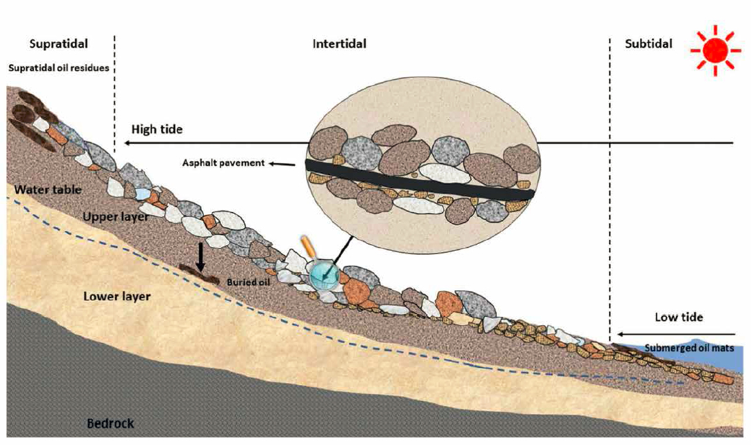
SOURCE: Wang et al. (2020).
that washover suspension of oil resulted “in the deposition within washover fans and channels in the supratidal portion of the beach.” These results show that crude oil aggregates could move across the beach by physical transport processes as well oil transport from intertidal and subtidal sediments.
On coarse sediment beaches, small amounts of oil can remain for decades in the intertidal zone. Oil that survives natural attenuation on the scale of weeks to months will likely remain on the beach in the form of tar mats, asphalt-like pavements, or as veneers on coarse particles or hard substrate until the environmental conditions shift (Curtis et al., 2018). Subsurface oil residues can penetrate into the pore spaces of the particles until it reaches limiting layers such as fine-grained sediment, the water table, or bedrock. Small fractions of the residual oil stranded within the protected residues can continue to degrade (Curtis et al., 2018).
The hydrodynamic conditions in coastal areas exposed to recurrent contamination result in long-term persistence of deep oil spills from wrecks by burying and resurfacing the oil in the intertidal zone (Bernabeu et al., 2013). Beach geomorphology contributed to the persistence of subsurface oil in a tidally influenced gravel beach of Prince William Sound (Alaska) polluted by the 1989 Exxon Valdez oil spill; the oil plume moved alongshore, which was attributed to the gradual slope and smooth substrate of the beach in that particular area (Xia and Boufadel, 2011). Oil biodegradation is sensitive to both nutrient concentration and biomass concentration (see Section 5.2.8). The surface area of sediments is a key parameter for microbial growth in sediments (Torlapthi and Boufadel, 2014): fine-grained sediments with little porespace for oxygen and nutrient diffusion can slow down the biodegradation processes in near shore environments (Pardue et al., 2014).
Residual oil from the DWH spill in the shallow surf-zone in the northern Gulf of Mexico was found primarily in two forms—as SOMs (Michel and Bambach, 2020) and surface residual balls (SRBs; see Box 5.10). Mats formed when weathered oil at the surface reached a shallow location that was energetic enough for waves to mix the sediment with the oil creating a sand and oil mixture (Plant et al., 2013). The mousse interacted with the sediment-oil mixture near the shoreline and sank to the bottom, forming SOMs. Over time, SOMs were buried, exposed, and broken apart through natural coastal process dynamics, and appeared as SRBs in the beach system, with sizes ranging from a few millimeters to several centimeters (Hayworth et al., 2015; Gustitus and Clement, 2017). SRBs (often referred to as “tar balls”) that formed after the DWH event, and found on northern Gulf of Mexico beaches, were different from traditional tar balls. DWH SRBs were a brownish, sticky substance with a strong odor of petroleum as opposed to the more extremely weathered tar ball (dark, either rubbery or hard, and without odor) more commonly seen (Hayworth et al., 2011; OSAT-2, 2011; Michel et al., 2013; Mulabagal et al., 2013; Yin et al., 2015).
Re-surveying the shoreline 13 years after the Exxon Valdez oil spill at 39 sites in Prince William Sound showed that, despite evidence of oil weathering, the natural weathering rates were slow both at the surface and in the subsurface (Taylor and Reimer, 2008; Li and Boufadel, 2010). The slow weathering was due to oil residue being mixed in with finer sediments and remaining sheltered on the shoreline from wave dynamics and other active weathering processes (e.g., the oil was isolated by boulders and outcrops or shallow bedrock formations). Persistence of subsurface Exxon Valdez oil extending into the biologically productive middle and lower intertidal zones after 12 years confirmed the potential for long-term biological effects on beaches most heavily impacted by the spill (Short et al., 2004, 2006). Surveys conducted after 16 and 20 years showed similar results, namely that stranded oil in subsurface sediments of exposed shores and subsurface oil may persist for decades with little change (Short et al., 2007; Boehm et al., 2014). In contrast, the half-lives of aliphatic and aromatic hydrocarbons in Macondo oil from the DWH spill that impacted Pensacola Beach (Florida) sands were 25 and 22 days, respectively, and aerobic biodegradation removed oil to background concentrations within one year (Huettel et al., 2018). Gros et al. (2014) determined that the dominant alkanes remaining 12–19 months after the spill were >C22, with the smaller alkanes presumably having been weathered and/or degraded in situ. Saturates in the C22–C29 range were partially depleted in the order n-alkanes > methylalkanes and alkylcyclopentanes + alkylcyclohexanes > cyclic and acyclic isoprenoids, consistent with other oiled aerobic environments. Even components of buried oiled sand patties, known to resist biodegradation, were being metabolized and incorporated into microbial biomass 5 years post-spill (Bostic et al., 2018). Bociu et al. (2019) estimated that golf ball–sized SOAs (see Box 5.10) embedded in sandy beaches were being weathered and aerobically degraded on north Florida beaches. They estimated that, although decomposition of the SOAs would take at least 32 years, in the absence of sediment contact the SOAs would persist for more than 100 years; therefore, incorporation of sand accelerated oil removal because of the porosity afforded by incorporated sand. Collins et al. (2020) similarly determined that the half-life of PAHs in Macondo oil buried in the intertidal zone depended on the flux of oxygen into the sediments and the permeability of the sediments. Nutrient permeation in some beach sediments may be augmented by natural microbial nitrogen fixation (Shin et al., 2019b), and the availability of nutrients (particularly nitrogen and phosphate) in oiled beach sand may influence which hydrocarbon-degrading species dominate—alkane-degrading Alcanivorax or PAH-degrading Cycloclasticus (Singh et al., 2014). Other factors in bioremediation on beaches are moisture and salinity: Elango et al. (2014) observed that PAH and alkane biodegradation rates were negatively affected in the intertidal zone where salinity was high and oxygenation was low, whereas in the supratidal zone nutrients and moisture limited biodegradation of stranded oil:sand aggregates.
The DWH spill posed challenging shoreline oiling characteristics (Michel et al., 2013). The normal erosional and depositional processes of the beach cycle and seasonal wind patterns caused the oil to become buried, exposed, and re-mobilized. Oil became stranded on beaches in three zones (i.e., supratidal, intertidal, and intertidal/nearshore subtidal zones). In the supratidal zone (see Figure 5.37), oil was stranded in patches by storm waves. In the intertidal zone, SRBs and SRPs became buried (0.1 m in places). Tropical storm Lee and Hurricane Isaac resulted in extensive beach erosion and release of oil residues. As described by Michel et al. (2013), two different patterns of oil accumulation occurred in the lowest intertidal/nearshore subtidal zone: (1) Along the more heavily oiled sand beaches along the northeast Gulf of Mexico, some of the oil/sand mixture accumulated in the nearshore subtidal areas, forming extensive SOMs (between the toe of the beach and the first offshore bar) which were recurrently buried and exposed by sand transport. As the SOMs broke up, they became persistent sources of SRBs/SRPs on the neighboring shoreline (see Figure 5.38); (2) Along most of the marshes, the stranded oil spread into the marsh with tidal currents due to high density of vegetation and the high viscosity residual oil (Michel et al., 2013). Salt marsh sediments are typically anaerobic below the surface and the presence of oil plus sulfate from tidal water supports anaerobic biodegradation through sulfate reduction (Natter et al., 2012), leading to production of high sulfide concentrations that can negatively affect marsh plants (Mills and McNeal, 2014). However, biodegradation of weathered Macondo oil was observed in sediment cores 18–36 months after the DWH oil spill, indicating that recovery of salt marsh sediments was occurring (Atlas et al., 2015). This observation was supported by detection of progressively oxygenated compounds assumed to represent metabolites from biodegradation of Macondo oil (Chen et al., 2016). ‘Omics surveys of marsh grass sediments suggested that the rhizosphere communities (microbes associated with plant roots) may have contributed to oil biodegradation in Gulf of Mexico salt marshes (Beazley et al., 2012). However, in coastal environments these oxygenated
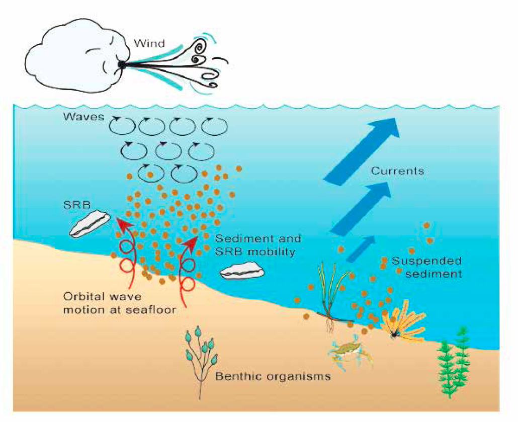
SOURCES: Plant et al. (2013); USGS.
hydrocarbons accumulate and may be recalcitrant to further degradation (White et al., 2016), emphasizing that simply monitoring the “disappearance” of parent hydrocarbons does not mean the partially oxidized metabolites or photochemical by-products have been removed from the environment. The fate of oxygenated hydrocarbon species and their effects in coastal ecosystems require additional study.
Beach oiling from the DWH spill showed oil contamination on the surface and buried below surface sands in the form of tar balls, tar patties, tar cakes, oil sheet, and stained sand (Wang and Roberts, 2013). The cross-shore distribution of surface oil was bound landward by the maximum high-tide wave run-up, which was, in turn, controlled by the incident wave condition. The dynamic and continual swash motion on the foreshore prevented preservation of surface oil deposition. The burial of oil contaminants was driven by the same processes as the initial surface deposition resulting in layers of oil contaminants that varied in both thickness (up to 15 cm) and depth (up to 50 cm). As the beach erodes, these buried oil contaminants can naturally resurface; alternatively, buried oil can also be removed through excavation.
The rate of PAH weathering decreases significantly once the oil becomes buried in sand or trapped within the SRBs. Chemical data indicate that submerged oil containing heavy PAHs (e.g., parent and alkylated chrysenes) can remain in the beach system for several years (Yin et al., 2015). Numerical analyses confirm that spatial distribution of infiltration flux due to waves was dependent on the large-scale hydraulic gradient at the beach and high landward water table reduced wave-engendered seawater infiltration. The decrease in seawater infiltration can have adverse effects on chemical transformation processes (e.g., nutrient recycle and redox condition) in beaches, and subsequently on receiving water bodies (Geng and Boufadel, 2015). Using measurements that integrated oil chemistry, hydrocarbon degrading microbial populations, nutrient and DO concentrations, and fundamental beach characteristics, Geng et al. (2021) found that “intrinsic beach capillarity along with groundwater depth provides primary controls on aeration and infiltration of near-surface sediments, thereby modulating moisture and redox conditions within the oil-contaminated zone.” Hypersaline sediment environments in beach pore water inhibited oil decomposition along the Gulf shorelines.
The knowledge gained since the Exxon Valdez and DWH spills on the interaction of mineral particles with stranded oil was a significant step in understanding the behavior and fate of oil in different coastal environments, particularly with low physical energy levels (Owens and Lee, 2003; Michel and Rutherford, 2014; Tarpley et al., 2014; Evans et al., 2017; Curtis et al., 2018; Owens et al., 2018). The interaction of especially fine mineral particles with stranded oil in coastal areas decreases the potential for oil to adhere to solid surfaces such as sediments or bedrock. The formation of stable, micron-sized oil droplets that disperse into the water column makes the oil more favorable for biodegradation, allowing the oil to be removed naturally in very sheltered coastal environments such as those with little to no wave action.
5.3.4.2 Tar Balls
Tar balls, tar mats, and tar patties are types of marine tar residues and can range in size from millimeters in diameter (tar balls) to several meters in length and width (tar mats) (Warnock et al., 2015; also see Figure 5.27). The term “marine tar residue” refers to different types of weathered oil conglomerates that can be found on beaches, the open ocean surface, and the seabed. Tar residues from the ocean surface or seafloor can be transported to the shore by waves and currents and deposited on sediments and beaches. Tar ball deposition on a beach depends on several factors such as a recent oil spill, ocean currents, winds, natural seeps, and tanker traffic. The appearance of new tar balls may indicate the occurrence of a recent oil spill.
Tar balls and patties can be transformed by several factors and it is difficult to determine how long they will retain form.4 Tar balls can break open from turbulence in the water such as beach activity, or directly though interaction with animals, exposing less weathered centers (more fluid and sticky). Tar balls also become more fluid and sticky as air and water temperatures rise. The amount of sediment present can have the opposite effect by adhering to the surface and hardening the tar ball, making it more difficult to break open.
5.3.5 Arctic Marine Systems and Sea Ice
Polar oceans historically have not been impacted greatly by accidental oil spills (see Chapter 3), but with decreased Arctic sea ice extent there has been increased shipping, tourism and interest in off-shore oil exploration, production and transportation in Arctic waters around Greenland, Canada, Alaska, Norway, and Russia (Brakstad et al., 2018a; Lewis and Prince, 2018). The possibility of increased frequency of oil spills coupled with vulnerability to global climate change (de Sousa et al., 2019), rapid ocean warming (Grossart et al., 2020), and a dearth of baseline information about the unique Arctic marine environment (reviewed by Lee et al., 2015) makes it imperative to consider the impact and fate of oil spills in this generally pristine environment. The U.S. Arctic Research Commission5 and the international Arctic Council6 are stakeholders in this endeavor. Studies conducted under the international Joint Industry Programme7; and SINTEF8 have included in situ mesocosm experiments
___________________
4 See https://response.restoration.noaa.gov/oil-and-chemical-spills/oil-spills/resources/tarballs.html.
5 See https://www.arctic.gov.
6 See https://arctic-council.org/en.
7 See http://www.arcticresponsetechnology.org/research-projects.
8 See https://www.sintef.no/projectweb/jip-oil-in-ice/publications.
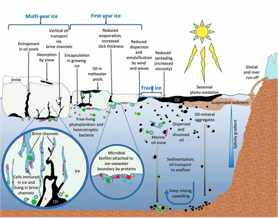
NOTES: Sea ice affects oil slick thickness by reducing surface spreading, by “herding” oil into pools and by encapsulating oil within ice masses; it also reduces mixing by waves and wind, decreasing natural dispersion of oil into suspended droplets. At the surface, oil can spread on meltwater pools or be absorbed by snow cover where it is subject to photo-oxidation. Glacial and river runoff provide fresh water, establishing a salinity gradient in the water column, and suspended sediments that may form oil-mineral aggregates (see Section 5.3.2) and sink to the seafloor. Deep mixing and upwelling can replenish nutrients from deep water. Seasonal solar irradiation photo-oxidizes floating oil and supports free-living phytoplankton and cyanobacterial communities that form marine snow and can interact with dispersed oil to form marine oil snow (MOS) that eventually sinks to the seafloor. Bacteria and plankton form biofilms on the underside of sea ice by attaching via extracellular polymers, and also may become entrained in brine channels. They may encounter oil in the water column, at the seawater:ice interface, or within ice masses. Bulk oil may migrate vertically through sea ice, especially during melting as it displaces brine in channels, and also may travel laterally when immured in drifting ice, and dissolved oil components may diffuse via brine channels.
SOURCES: Committee generated; adapted from NRC (2014) and Vergeynst et al. (2018).
and field trials addressing various aspects of Arctic oil spill research and response.
Most of the same factors that affect the fate of spilled oil at lower latitudes also affect polar marine environments, but some are magnified and some are unique to polar oceans (see Figure 5.39). Briefly, these include (1) seasonally low air temperatures and constantly low water temperatures that affect oil behavior and chemistry by increasing its viscosity; (2) seasonal ice cover that reduces mixing of water by wind and wave action, thus indirectly decreasing dispersion and emulsification of floating oil (see Sections 5.2.2 and 5.2.7), and also resulting in stratification of water layers by salinity (density) more so than by temperature; (3) extreme seasonal differences in solar input that directly affect oil photo-oxidation of oil (see Section 5.2.5) and also influence seasonal phytoplankton blooms that can accelerate oil sedimentation (see Section 5.3.2); (4) seasonally low dissolved nutrient concentrations affected by sequestration in phytoplankton blooms and salinity stratification; (5) seasonal increases in suspended sediment plumes from glacial and
river runoff that affect sedimentation of oil associated with particulates (see Section 5.3.2); and (6) generally pristine conditions in which hydrocarbon-degrading microbes are relegated to the “rare biosphere” (see Section 5.2.8.2) with some exceptions, such as natural bitumen seeps on the Mackenzie River that runs to the Arctic Ocean (Carey et al., 1990) and point-source natural sub-sea seeps (see Section 5.4.1). These factors and their consequences for oil properties and fates are discussed in greater detail below, first by describing the effects of temperature and sea ice on oil behavior and chemistry (see Section 5.3.5.1), their effects on biodegradation (see Sections 5.3.5.2 and 5.3.5.3), and other pertinent factors in the water column (see Section 5.3.5.4) and in Arctic seafloor sediments and shorelines (see Section 5.3.5.5).
5.3.5.1 Effects of Low Temperatures and Sea Ice on Oil Behavior and Chemistry
The most obvious characteristics distinguishing polar marine environments from temperate oceans are constant low temperature and presence of seasonal and permanent sea ice (frazil ice versus first- and multi-year ice). Notably, the Arctic water column is predominantly stratified by salinity rather than temperature. Wind and wave mixing of surface waters (which have low salinity due to river inputs, seasonal sea ice, and glacial melt runoffs) with denser, higher-salinity deep waters is reduced under ice cover. Thus, unlike the steep and seasonal temperature gradients characteristic of temperate oceans, the Arctic ocean temperature has a shallow temperature gradient that does not change markedly with either season or depth. Surface water temperatures typically range from -1.8°C in winter (the freezing point of seawater) to ~8°C in summer and from -1.2–4°C in deep Arctic waters (> 500 m depth) (Vergeynst et al. 2018b).
Temperature Effects
Low temperature affects oil behavior and chemistry (reviewed by Dickins, 2011; Lee et al., 2011a; Vergeynst et al., 2018) by increasing oil viscosity, with complicated consequences. Greater viscosity slows oil spreading on water and produces thicker films, resulting in a smaller impacted surface area than in temperate open waters. (Ice and snow further reduce oil spreading, as discussed below.) The thicker slicks have decreased photo-oxidation potential that may be offset by high seasonal insolation at high latitudes. Thicker slicks and cold air temperatures decrease evaporation rates, allowing toxic low molecular weight components to persist longer in the oil where they may be available to dissolve into the water column. However, dissolution is balanced by greater viscosity that reduces oil droplet size (a balance between dispersion and coalescence) and decreases both dissolution and biodegradation due to smaller oil:water interfacial area. Additional temperature effects on dissolution include the water solubility of hydrocarbons, which generally decreases until a critical temperature range is reached (usually between 0°C and 30°C), then slightly increasing. Temperature also affects molecular dispersion: a drop in water temperature from 10°C to 0°C decreases diffusion of low molecular weight alkanes (≤C5) by ~20% (Michalis et al., 2016). Crude oils with high wax content can gel at low temperatures, changing spreading and evaporative behavior (reviewed by Potter et al., 2012).
Thus, cold temperature overall decreases loss of bulk oil by physical weathering processes so that water temperatures near freezing may prolong exposure of local marine biota to toxic low molecular weight water-soluble oil components such as aromatic hydrocarbons compared with temperate waters. There has been speculation that dispersants would be ineffective in cold Arctic waters, but Lewis and Prince (2018) concluded that water temperatures as low as 0–2°C generally do not preclude dispersant effectiveness (see Section 4.2.3.4).
Ice Effects
Although transportation of both floating oil and ice are affected by the same driving forces of wind and currents, ice coverage affects oil behavior and chemistry in additional ways (reviewed by Fingas and Hollebone, 2003; Buist et al., 2008; Potter et al., 2012): (1) sea ice physically restrains oil from spreading on water (sometimes by orders of magnitude; Vefsnmo and Johannessen, 1994), and can concentrate oil in leads between floes, thereby reducing the area of slicks and decreasing evaporative losses of low molecular weight components from slicks; (2) sea ice decreases wave energy and surface water mixing (Brandvik and Faksness, 2009), which in turn decreases emulsification and dispersion, increases droplet size in the water and thereby decreases bioavailability; (3) sea ice, whether present as frazil, first-year, or multiyear ice, influences light penetration and photo-oxidation, with consequences for oil chemistry, toxicity, biodegradation, and algal growth; and (4) sea ice can entrain floating oil and transfer it both vertically through the ice, as described below, and horizontally with pack ice, often moving in a different direction from the underlying currents.
Sea ice comprises pure ice, gas bubbles, brine-filled channels, solutes and entrained particulates including living and dead microorganisms and their polymers (EPS), organic detritus and mineral particles (Meiners and Michel, 2017). Unlike freshwater ice, sea ice is porous, having an internal network of fluid-filled channels as a consequence of brine exclusion while the ice is forming. The bottommost pores are directly in contact with the underlying seawater and permit exchange of fluids (including oil) between the water column and ice. As described by Wang et al. (2017), sea ice acts as “a dynamic and porous ‘lid’ between the atmosphere and the ocean [acting] as both a temporary storage and an effective transporter for contaminants, moving them in space (vertically between the atmosphere and the ocean, and laterally
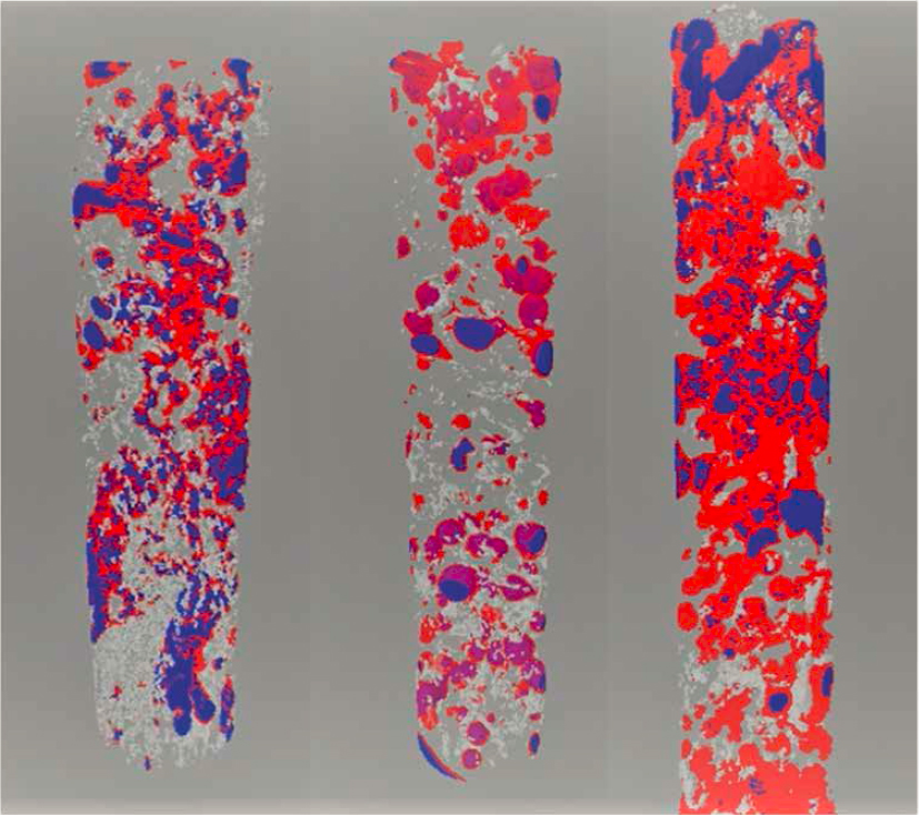
SOURCE: Desmond et al. (2021b), supplementary information.
as ice drifts) and in time (seasonal storage and release via freeze and melt).” The extent of oil movement within the ice differs according to the age and temperature of the ice. Recent x-ray micro-computerized tomography (CT) studies of oil, air and brine distribution in artificial sea ice cores revealed that bulk oil injected beneath the ice migrated toward the surface and became occluded within the ice, sometimes as pockets and often surrounding the perimeter of air inclusions (Desmond et al., 2021b; see Figure 5.40). In contrast, the oil had minimal interfacial contact with brine, suggesting that oil progressively displaced and replaced brine as it percolated through the channels and became encapsulated in the ice. If this mesocosm study translates to natural sea ice, physical separation of oil and brine likely has consequences for biodegradation, since bacteria are associated with the brine. Microbial contact with oil then would primarily occur at the base of the ice or in melt ponds rather than within the ice mass, or in warm ice (> -5°C) when channels are larger. The separation of oil and brine also reduces dissolution of hydrocarbons into water due to their reduced interfacial areas, affecting biodegradation potential within cold ice (Desmond et al., 2021a). In addition to movement of bulk ice, dissolution and diffusion of oil components also occurs: in an in situ mesocosm study in Svalbard, Boccadoro et al. (2018) noted that PAHs, as opposed to alkanes, in a light crude oil applied to first-year ice surface migrated to the underlying water column via dissolution. The commissioning of the new Ocean–Sea Ice Mesocosm (OSIM) facility at the Churchill Marine Observatory (CMO) on Hudson Bay9 in 2022 will provide infrastructure for examination of oil–sea ice interactions.
Frazil ice comprises newly forming, randomly oriented ice crystals, occurring usually in supercooled water under turbulent conditions and often where pack ice meets open ocean and where microbial primary productivity is greatest (Lofthus et al., 2020). In the process of consolidation of frazil into first-year ice, solutes, cells, and particles can become encapsulated rapidly—within hours to days (Potter et al., 2012)—as can floating oil or suspended oil droplets near the surface. Floating oil can also penetrate the bottom of pre-existing first-year ice. Petrich et al. (2013) estimated from field samples that < 2 L crude oil might be entrained per square meter of cold first-year ice in winter, and 5–10 L/m2
___________________
9 See https://umanitoba.ca/environment-earth-resources/earth-observation-science/marine-observatory.
entrained in warmer ice in spring. The oil overridden by ice can then be transported vertically via brine channels to the ice surface and atmosphere during spring melt. Oil spilled under multi-year ice can be retained by the rough ice at the water:ice boundary, creating relatively thick pools (reviewed by Potter et al., 2012) with little penetration into the ice. Conversely, oil that is encapsulated during ice growth subsequently can be exposed and released to seawater during ice melt (ablation) as brine channels drain (Oggier et al., 2020). The extent of entrainment and transport depends on the type and thickness of ice and particularly its porosity (percent of volume occupied by brine channels), both of which are influenced by ambient air temperature (Faksness and Brandvik, 2008a). Warmer ice is typically more porous and, as the ice deteriorates in spring, the channels within may exchange brine for floating oil. Colder ice may simply encapsulate oil until seasonal warming enables migration, or may transport oil vertically as much as 30 cm (Oggier et al., 2020). Oil may persist in multiyear ice for up to 5 years or seasonal melting may release the oil from first-year ice to impact the food web at a distance from the original location, since sea ice movement can be a major pathway for long-distance cryptic transport of entrained oil (Wang et al., 2017). Recent modeling of the transport and weathering fates of the PAH naphthalene predicted a low potential for incorporation into a hypothetical Arctic food web (Oliveira et al., 2019), but the authors caution that there is limited knowledge of the ecological effects of oil spills in ice-covered waters.
Oil incorporated into sea ice contacts hyper-saline brine, which decreases water solubility of aliphatic and aromatic hydrocarbons by 3- to 60-fold (reviewed by Vergeynst et al., 2018; Table 2 in Saltymakova et al., 2020) and influences the hydrocarbon content of brine released to the ocean during ice melt. This can lead to chromatographic separation of water-soluble oil components as oil migrates through brine channels and air bubbles in the ice (Faksness and Brandvik, 2008b; Desmond et al., 2019; Saltymakova et al., 2020) and may also affect biodegradation (see Section 5.2.8). Boccadoro et al. (2018) additionally determined experimentally that PAH migrated through the sea ice more effectively when dispersant was present, likely improving the otherwise-limited bioavailability. Sea ice cover thus serves as a reservoir for retention and migration of oil as well as particulates and solutes that support microbial activity, discussed below.
While the studies cited above provide detailed understanding of the fine-scale interactions of oil and ice and the possible breadth of these interactions and their impact on oil fate processes, predicting response-scale transport of oil within ice-infested waters is exceedingly difficult at present. Accurate predictions would require knowledge of the detailed under-ice topology, the ice porosity, density of surrounding seawater, and many other small-scale aspects of the ice. This is especially difficult since ice and the surrounding seawater may be moving at different velocities and because the ice is dynamic, undergoing a myriad of changes over time. Current models for oil transport assume that oil transports with the drift ice field when ice coverage is 70% to 80% or greater, that oil moves as it would be in open water at drift ice coverages of 20% to 30% or less, and the oil moves at a linear interpolation of these two extremes for intermediate ice coverages. Some models also use these percentages to scale fate processes for interaction with the atmosphere. The real situation may be much more complex, dependent on the actual in situ ice properties and coverage and their interactions with local currents. Hence, though there is a good understanding of the fine-scale interaction of oil with ice, models have imprecise ice predictions and must average over large scales so that simplified approaches are required to predict oil–ice behavior. Development of these algorithms require validation data and will likely rely on real-time data integration of observing systems during future spills.
5.3.5.2 Effect of Low Temperature on Oil Biodegradation
In the event of an oil spill, the remoteness of some Arctic regions would delay and alter spill response options some of which, furthermore, would be less effective due to local conditions (see Chapter 4). Biodegradation (via natural attenuation) might then be the primary or the only feasible fate of spilled oil, and onset of that activity might be delayed because most Arctic sites are historically pristine. The Arctic Monitoring and Assessment Programme (2010) has estimated that 95% of hydrocarbons in Arctic oceans (~4 × 10⁴ tons crude oil per year) are associated with point-source natural seeps rather than with spills. Therefore, aside from localized exposure to hydrocarbons at seeps (Cramm et al., 2021; see Section 5.3.5.5) and associations with hydrocarbon-synthesizing phototrophs (see Section 5.2.8), there is little selective pressure to enrich or maintain hydrocarbon-degrading bacteria for recruitment to spilled oil, and they are typically part of the “rare biosphere” (see Section 5.2.8.2). This paucity might increase the lag time before biodegradation becomes significant, although the rates of biodegradation may then be relatively fast, as discussed below. In addition to their importance for oil removal, microbes are at the base of the Arctic food web (reviewed by Kellogg et al., 2019) and any effects on their metabolism will impact higher organisms. Unfortunately, due in part to the difficulty of accessing remote northern sites for scientific sampling, until recently the application of ‘omics techniques to polar marine regions has lagged behind studies of temperate marine environments, and further research effort is needed to augment understanding of Arctic ecosystem responses to oil (Lauritano et al., 2020; Zhong et al., 2020). Current Canadian endeavors in Arctic ‘omics include GENICE (Microbial Genomics for Oil Spill Preparedness in Canada’s Arctic Marine Environment) and the MPRI (Multi-Partner Research Initiative; Lee, 2021).
Temperature affects all biological processes although, surprisingly, it may have less impact on Arctic oil biodegradation
than expected because (1) O2 solubility increases with decreasing water temperature and (2) the temperature gradients observed in temperate water columns are not as steep in polar oceans and the native microbiota are adapted to constant cold temperature throughout the water column. Broadly accepted terms describing microbes adapted to cold are: “psychrotolerant” or “psychrotroph” for those that grow optimally at temperatures >15°C but tolerate and grow at lower temperatures; and “psychrophile” for organisms that die at >20°C, grow optimally at ≤15°C, and can be metabolically active below 0°C (Moyer and Morita, 2007). Psychrotrophs are quite common in diverse environments and many of the recognized oil-degrading microbes in Arctic oceans are psychrotolerant, whereas true psychrophiles are rarer and restricted to constantly cold environments such as deep oceans and polar regions. Oil-degrading genera that are commonly detected by polar marine studies during low-temperature biodegradation include members of the family Oceanospirillaceae such as the psychrophilic obligate hydrocarbon-degraders Oleispira antarctica, Oleiphilus, and Thalassolituus; psychrotolerant heterotrophs Polaribacter, Colwellia, and Cycloclasticus and the recently detected Zhongshania and Paraperlucidibaca (see Appendix I). ‘Omic surveys of microbiomes in Canadian Arctic seawater, sediment, shorelines, and deep seeps have revealed ubiquitous distribution of hydrocarbon-degrading species in the rare biosphere (C. Hubert, personal communication) that are enriched when incubated with oil in vitro. Comparison of sequences to the global Tara Oceans database (Sunagawa et al., 2015) indicates that some key hydrocarbon-degrading taxa, such as the latter two listed above, are endemic to polar marine environments but rare in lower latitudes (Murphy et al., 2021); conversely, other keystone species are more common in temperate marine environments. Recognition of key endemic species could inform response decisions and interventions might be tailored to enrich polar-specific oil-degrading species.
When temperature is invoked as a limiting factor for microbial metabolism, the concept of Q10 based on the Arrhenius equation is often applied to whole organism (or community) metabolism. Briefly, the Q10 rule of thumb states that, below the optimum temperature for an activity (an individual enzyme or microbial cell growth), a reduction of 10°C results in a 2–3-fold reduction in the rate of that activity. This generalization is incorporated into some numerical models for the fates of oils. However, cold-adapted microbial communities may not conform to this rule, which was developed primarily to describe in vitro enzyme reaction rates at moderate temperatures. Therefore, the relationships between temperature and rate of oil biodegradation or pattern of susceptibility to biodegradation are not straightforward. Because temperatures are low but constant in Arctic marine waters, the magnitude of the Q10 effect is dampened because the microbiota are adapted to low temperature; therefore, extrapolating Q10 values from temperate water data may be invalid (Vergeynst et al., 2018). Furthermore, applying a universal Q10 factor to different oil spill conditions is questionable because the metabolic rates of key genera (e.g., Alcanivorax and Cycloclasticus) have not been determined experimentally under temperature and nutrient concentrations relevant to cold marine environments (Bagi et al., 2014). Meta-analysis of 10 published datasets indicated that models using correction factors based on the Arrhenius equation underestimated in situ oil biodegradation rates and that lag time before onset of biodegradation (which is accommodated differently by different models) was inversely influenced by temperature (Brown et al., 2020). More specifically, Nordam et al. (2020) examined Q10 scaling for biodegradation of individual oil components at four temperatures spanning –2°C to +13°C. They found that conventional Q10 scaling was adequate for predicting biodegradation rates for the more water-soluble, lighter oil components, but were less accurate for poorly water-soluble, higher molecular weight oil components, possibly because Q10 does not capture temperature effects on oil behavior (e.g., increased viscosity and decreased water solubility of PAHs at low temperature; reviewed by Margesin and Schinner, 2001). Based on these and other reports, best practices would then require that experiments be conducted at temperatures relevant to in situ conditions, rather than being extrapolated from data collected at moderate temperatures, and that alternative approaches be developed to predict low-temperature biodegradation rates.
Unsurprisingly, there are numerous reports that oil biotransformation rates are slower at cold than at moderate temperatures (e.g., Prince et al., 2013) but there are also reports of unexpectedly rapid biodegradation at low temperature. Laboratory and in situ experiments using cold deep waters and warmer surface waters collected near the DWH site found that PAHs degraded slightly faster at 4°C than at 24°C and n-alkane degradation was only marginally faster at the higher temperature (Liu et al., 2017). Interestingly, the deep-sea microbial community outperformed the surface community at both temperatures. Thus, temperature may not be as important in cold ecosystems as co-existing factors like seasonal nutrient concentrations (see Section 5.3.5.4) and oil bioavailability (see Box 5.5). However, even this generalization is inadequate, as temperature may affect degradation of aliphatics differently than aromatics in some cases. Kristensen et al. (2015) examined crude oil biodegradation in cold Arctic and warmer North Sea water samples and found that the order of biodegradation of oil classes differed at the two sites, with aliphatics being preferentially degraded before PACs in Greenland seawater incubated at 5°C versus the opposite pattern of faster PAC biodegradation in Danish seawater incubated at 15°C. That is, preferences were site-specific, providing a cautionary lesson about generalizing hydrocarbon biodegradation susceptibility in cold waters. Scheibye et al. (2017) also observed biodegradation of n-alkanes (C13–C30) in deep Greenland seawater at 2°C, but losses of (alkyl) PACs were attributed to abiotic dissolution rather than biodegradation. Lofthus et al. (2018) incubated
thin films of oil adsorbed to a support fabric in seawater at temperatures from 0°C to -20°C and found that the n-alkane biotransformation rate decreased at lower temperature, likely due to physical changes in the oil. Biodegradation has been observed in seawater even at sub-zero temperatures: chemically dispersed diesel fuel was incubated with seawater from Norway (after enhancing salinity to depress the freezing point) at -2°C and -6°C (Dang et al., 2020). Although chemical dispersion of diesel would not be a response option in situ, the experimental observation of significant degradation of n-alkanes (nC10–nC36), decalin, and 2–5-ring PACs at these low temperatures expands the permissive temperature range for hydrocarbon biodegradation.
5.3.5.3 Biodegradation Within and Below Sea Ice
Sea ice, and particularly liquid brine channels within the ice, presents an extreme habitat for microbial life, imposing combinations of stressors including limited diffusion of nutrients, seasonally fluctuating salinity from near freshwater to hypersaline (200 ppt) and fluctuating low temperatures from -1 to < -20°C. Nonetheless, sea ice harbors communities of microbes and viruses recruited from, yet distinct from, those in sea water (Fernández-Gómez et al., 2019; Zhong et al., 2020) and provides a niche for assembly of microbial biofilms both within and under the ice (see Figure 5.41). Furthermore, sea ice is not merely a refuge for dormant microbes: bacterial metabolism has been detected within Arctic sea ice at temperatures as low as -20°C (Junge et al., 2004), particularly in microbes physically associated with other cells such as algae or with inorganic particles or ice crystal faces. Because of these physicochemical stressors, microbial communities in bulk sea ice are less dense and less diverse than in sea water (Yergeau et al., 2017) whereas microbes, solutes, and other particles are concentrated in brine channels by exclusion as ice forms from seawater (Zhong et al., 2020), during which cold-adapted microbes are enriched (Deming and Collins, 2017). Reported densities of bacteria in sea ice range from 103 to 107 per mL of bulk ice, or up to 108 cells per mL of brine fluid, although not all of the cells may be active at sub-zero temperatures. Cooper et al. (2019) visually counted ~105 cells per mL of sea ice brine, ~5% of which were dividing; virus-like particles were also noted at virus:cell ratios of 0.7–3. Yergeau et al. (2017) used metagenomics (see Section 5.2.8.1 and Appendix H) to determine that distribution of microbes and genes was uneven in sea ice, with greater microbial numbers being detected at the bottom of the ice columns near the ice:water boundary. Virus (particularly bacteriophage) densities range from 104 to 108 units per mL in bulk ice (Deming and Collins, 2017) but their activity in situ is not well known. Notably, most studies to date have been conducted in frazil and first-year ice rather than multi-year ice (reviewed by Deming and Collins, 2017), highlighting another knowledge gap.
The value of in situ experiments is demonstrated by a pair of Arctic field studies examining the fates of aliphatic and aromatic components of three oils: marine gas oil (a diesel distillate), a blended North Sea crude oil, and a high-sulfur intermediate fuel oil. In the first study (Vergeynst et al., 2019a) the oils were sorbed to mesh supports and incubated in Greenland fjord water during the summer months. The oil was depleted by a combination of evaporation,
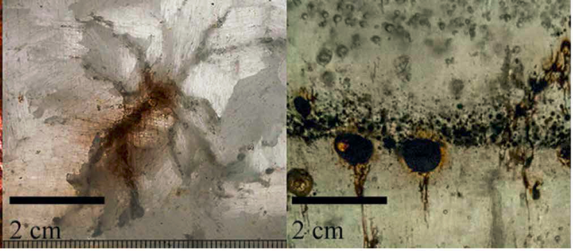
SOURCE: Adapted from Oggier et al. (2020).
photo-oxidation, dissolution and biodegradation, with the latter being the dominant fate for alkanes and PACs concurrent with development of an enriched bacterial biofilm on the mesh. Among the abiotic fates, evaporation accounted for early losses of short-chain alkanes, dissolution accounted for early depletion of two- and three-ring PACs and photooxidation depleted high-molecular weight PACs. Overall, dissolution and photo-oxidation of PACs were more important fates for marine gas oil and the crude oil, whereas dissolution and biodegradation processes dominated PAC depletion from the fuel oil. In the companion study (Vergeynst et al., 2019b), mesh supports with sorbed marine gas oil were frozen into first-year ice, extending into the underlying sub-zero Greenland fjord seawater. Rapid biodegradation of n-alkanes in the sub-zero seawater occurred at rates comparable to those in temperate waters but degradation within the sea ice was negligible. Genomic analysis of the biofilms revealed that Oleispira antarctica (see Appendix I) was present in 25–100-fold greater abundance in seawater than in sea ice and likely contributed to the different n-alkane biodegradation outcomes. PAC depletion differed in seawater and sea ice, with dissolution occurring 3–6.5 times faster in seawater. Photo-oxidation was important in ice and the upper water column, increasing with increasing PAC alkylation and ring number. The experiment showed that sub-zero temperatures permit oil biodegradation in seawater, but severely limit biodegradation in sea ice at a similar temperature. The two studies highlight the need to measure oil weathering fates and rates in different compartments of ice-covered marine systems and to study different oil types separately.
Total microbiological activity associated with sea ice occurs primarily along the bottom of the ice (Boccadoro et al., 2018), and is dominated in spring and summer by photosynthetic microalgae (reviewed by Lee et al., 2011a; Bowman, 2015). Microbes attached to and living in ice near the ice-water contact zone produce metabolites that “sculpt” the ice, enhancing biofilm attachment and growth of the algae, and facilitating access to nutrients in brine channels. Thus, sea ice is a dynamic reservoir of active microbes, both photosynthetic and heterotrophic, and their associated viruses, originally sourced from seawater then concentrated and selected during brine channel formation.
Due to their location in the ice and water column, algae are likely to be adversely affected by floating oil, although the susceptibility of different species varies and some diatoms are more resistant to the effects of oil (Lee et al., 2011a); zooplankton that graze on the algae may be affected secondarily. Arctic phyto- and zooplankton experienced sub-lethal effects when exposed to water-soluble oil components at concentrations of 0.07–0.55 mg L–1 both with and without additional photo-oxidation (Lemcke et al., 2019) (see Section 5.2.5). Seawater below melting ice during the winter-summer transition in the Greenland Sea was found to harbor a naturally high abundance of hydrocarbon-degrading bacteria (Marinobacter and Alcanivorax; see Appendix I), perhaps sustained by biofilms on the underside of sea ice that comprise bacteria and marine algae, some of which synthesize alkanes. Thus, the underside of ice and the water in contact with it may enrich hydrocarbon-utilizing microbiota.
Microbial biofilms associated with the underside of sea ice (inset, Figure 5.39) are likely mediated by ice-binding proteins (IBP) that have been identified in various polar eukaryotic algae, fungi and bacteria. These extracellular microbial IBPs, unlike the intracellular antifreeze proteins of higher organisms, alter the structure and behavior of ice crystals, protect the cells against freeze-thaw damage, and facilitate attachment of secreting cells to ice surfaces and to IBP-free cells such as diatoms and microalgae, thus promoting the formation of symbiotic photosynthetic biofilms at the sea ice:seawater interface (Guo et al., 2017). By sequestering the cells near the top of the water column, they are optimally placed to access oxygen and nutrients from photosynthesis (Bar Dolev et al., 2016) and/or to contact floating oil or newly ice-embedded oil. Biofilm formation on the ice under-surface may also facilitate close interactions between alkane-synthesizing cyanobacteria and hydrocarbon-degrading bacteria as a source of competent microbes for recruitment in the event of an oil spill.
Within bulk sea ice, ‘omics has revealed the presence of putative hydrocarbon-degrading bacteria and associated genes (Bowman and Deming, 2014) even in the absence of oil, and exposure of ice to oil shifts the microbial community composition as key species increase in abundance (e.g., Garneau et al., 2016). In a winter field experiment at Svalbard designed to demonstrate emergence of selected species in response to oil, Brakstad et al. (2008) overlaid an oil slick with an ice slurry, which froze in place. The presence of oil increased the total microbial abundance 5-fold compared with unoiled ice, and the community composition of the clean and oiled ice diverged over several months as the key hydrocarbon-degrading bacterium Colwellia was enriched. Analysis of oil recovered from the ice did not conclusively demonstrate biodegradation in situ but did suggest slow biotransformation where the oil concentration was low (Brakstad et al., 2008). This field study demonstrated that bacterial communities exposed to oil could become enriched even in ice at sub-zero temperatures, even if biodegradation within the ice was slow or negligible.
The latter observation is interesting. Despite the presence of appropriate species and apparent community shifts in response to oil exposure, Lofthus et al. (2020) noted that no experiments to date have demonstrated substantial biodegradation of bulk oil within sea ice. Instead, losses of specific oil components have been detected in the bottommost portions of ice that are in contact with seawater; such losses might be attributed to a combination of dissolution and biodegradation (Boccadoro et al., 2018; Vergeynst et al., 2019a). The extent and pattern of losses also depended upon the type and concentration of oil in the ice and whether the oil had been weathered before becoming embedded,
thereby removing the most water-soluble and bioavailable components such as short-chain alkanes and monoaromatics; that is, perhaps only hydrocarbons dissolved in liquid brine channels are bioavailable in ice. Another factor proposed by Garneau et al. (2016) is that oil biodegradation in sea ice might be limited by a combination of low nutrient concentrations and relatively higher concentrations of labile dissolved organic matter, such as exopolymers produced by algae in the sea ice, which might be degraded in preference to the oil components. Yet another factor potentially limiting oil biodegradation in bulk ice might be access to the oil itself rather than survival, since Garneau et al. (2016) observed good biodegradation of oil by melted sea ice (indicating that appropriate organisms and sufficient nutrients were present in the ice), and in agreement with speculation by Desmond et al. (2021a,b) about partitioned distribution of oil, air, and brine in ice (see Section 5.3.5.1). Frazil ice with its high water:ice contact area differs physically from first- and multi-year ice, and might provide greater opportunity for oil biodegradation if it entrained floating oil while forming. Lofthus et al. (2020) examined the fate of weathered, chemically dispersed North Sea crude oil in frazil ice formed from seawater and held at -2°C. Over 125 d the presence of frazil ice enhanced n-alkane degradation and decreased two- to three-ring PAH degradation compared with parallel ice-free seawater controls. Despite depletion of some oil components, there was negligible loss of total oil regardless of ice because the biodegradable fraction of hydrocarbons represented only a small proportion of the bulk North Sea oil applied.
Thus, selective biodegradation of oil components may occur within cold sea ice at very slow rates that are difficult to distinguish from dissolution and evaporation. Given that biodegradation can occur at moderate rates in seawater at the same temperature, it is clear that other factors reduce biodegradation rates within the ice, such as decreased surface area (oil bioavailability); limited nutrient and/or oxygen diffusion; the presence of alternate labile carbon sources like exopolymers from biofilms; limited diffusion of substrates and/or metabolic products in brine channels for efficient distributed metabolism; and possibly hypersaline brine. However, as the ice warms, melts, and liberates the microbes and oil, biodegradation can occur in near-surface seawater or meltwater ponds on the ice or in expanded brine channels. Further laboratory and in situ studies are needed to examine this possibility.
5.3.5.4 Other Factors Affecting Biodegradation in the Arctic Water Column: Bioavailability and Nutrient Concentrations
As discussed in Section 5.3.5.1, low temperature increases oil viscosity and makes dispersion more difficult, leading to larger droplet sizes with smaller total oil:water interfacial surface area that in turn affects biodegradation rates by limiting bioavailability. As noted in Section 5.2.8.3, Brakstad et al. (2015a) showed shorter lag times and faster degradation of n-C10–21 alkanes and 2–3 ring PACs in 10 µm oil droplets than in 30 µm droplets at 5°C, whereas biodegradation of higher molecular weight alkanes (n-C22–36) and 4- to 5-ring PACs was slower but comparable in both droplet sizes. That is, as expected, greater surface area increased bioavailability of the more water-soluble oil components. Besides affecting dissolution, the interfacial area of droplets affects microbial community dynamics. In one experiment, larger droplets exhibited delayed succession of oil-degrading species in biofilms associated with the oil (Brakstad et al., 2015b). In another study, biodegradation proceeded only after biofilms had formed on the surface of the oil droplets; in fact, agitating the culture to decrease adherence delayed microbial growth. Once biofilms had formed, droplet size decreased and droplets disappeared with longer incubation time and disappeared (Deppe et al., 2005). Therefore low temperature, in addition to presence of sea ice damping surface mixing in Arctic waters, can indirectly affect oil biodegradation by influencing oil behavior.
Another parameter particularly affecting biodegradation in many Arctic waters is insufficient concentrations of nutrients (e.g., nitrogen) required for effective oil biodegradation. There are several reasons for this phenomenon. First, stratification occurs when low-salinity meltwater at the surface is not effectively mixed with underlying layers due to density and the seasonal damping effect of sea ice that decreases mixing by wind and waves: nutrients may remain at depth rather than at the surface where oil is spilled and degraded. Second, seasonal phytoplankton blooms may sequester nutrients in cell biomass during photosynthesis, even if they fix nitrogen (N2). As an example, total nitrogen (mainly nitrate) concentrations in deep Greenland waters (>100 m depth, below the photic zone) are commonly 10–18 µM year-round (reviewed by Vergeynst et al., 2018), but in the surface waters nutrient concentrations undergo a yearly cycle. In the photic zone (surface to 25–50 m depth), phytoplankton deplete dissolved nitrate to concentrations of ~0–5 µM in the spring and summer. In winter nitrate is replenished from below. This cycle may be amplified in polynyas and marginal ice zones (Vergeynst et al., 2018). Despite such sequestration, nutrient concentrations in seawater may be adequate to enable biodegradation of low concentrations of oil in the water column: McFarlin et al. (2014) incubated Alaska North Slope crude oil with Alaskan seawater at -1°C, without nutrient amendment but also with or without chemical dispersion, and measured significant biodegradation within 60 d. Subsequently, McFarlin et al. (2018) reported that surface seawater collected from the Chukchi Sea and amended with low concentrations of nutrients (approximating natural background conditions) not only aerobically biodegraded 36–41% of North Slope oil within 28 d at 2°C, but also significantly biodegraded the surfactant component of Corexit 9500. Colwellia, Polaribacter, and Oleispira were implicated in both oil and Corexit biodegradation and may in fact
have degraded dispersant components in preference to oil under the study conditions. Similarly, Gofstein et al. (2020) determined that crude oil components (in the order n-alkanes > iso-alkanes > PAHs) and the surfactant component of Corexit 9500 were degraded by Arctic seawater microbes, with some taxa specializing in one or the other substrate and others apparently able to degrade both.
5.3.5.5 Arctic Seafloor Sediments, Deep Seeps, and Shorelines
In a survey of seafloor sediments from a transect of the Arctic Ocean, Dong et al. (2015) detected 16 U.S. EPA priority PAHs in all assayed cores. The concentrations decreased with sediment sample depth and with location from southernmost to northernmost sites. Taxonomic analysis of 16S rRNA genes revealed the widespread presence of known hydrocarbon degraders commonly detected at lower latitudes, including Cycloclasticus, Alcananivorax, Colwellia, and Dietzia (see Appendix I), with the latter being most abundant. Notably, these genera degrade oil aerobically, whereas subsurface sediments typically are anaerobic; it is therefore unclear whether these cells were active or dormant in situ, even though they were still viable and could be isolated and/or enriched in the laboratory. Ferguson et al. (2017) incubated subarctic deep-sea sediments at 0°C and 5°C with a model oil comprising 20 hydrocarbons (representing saturates, monoaromatics, 3–4 ring PAHs and resin components >C8) in the presence and absence of the marine oil dispersant SuperDispersant 25. The sediment microbial community composition shifted during hydrocarbon degradation at both temperatures, and the dispersant had variable effects on biodegradation, from insignificant effects at 5°C to enhanced biodegradation at 0°C. The research concluded that the effect of dispersant was ambiguous, needing further investigation under cold conditions. In contrast to the aerobic PAH study, Gittel et al. (2015) specifically surveyed cold marine sediments for the presence of anaerobic alkane degradation genes, which are represented by some marker sequences in databases. They found the genes to be ubiquitous, along with nanomolar concentrations of short-chain alkanes even in sediments considered pristine. Taken together, the studies suggest that the potential for both aerobic and anaerobic alkane biodegradation is widespread in cold seafloor sediments, and there is cosmopolitan distribution of species and genes associated with oil degradation.
Cold hydrocarbon seeps support cold-adapted hydrocarbon-degrading bacteria that may be recruited to Arctic marine oil spills. A hydrocarbon seep recently sampled in Scott Inlet, Baffin Bay in the high Arctic, supported seafloor microbial mats and colonies of higher organisms, and the water column above and down-current of the seep were enriched in putative methane- and hydrocarbon-oxidizing bacteria, the latter including the genera Polaribacter and Colwellia (Cramm et al., 2021) commonly enriched during oil spills in cold seawater. Both aerobic and anaerobic methane-consuming microbes can exist at gas seeps. An Arctic cold gas seep in the Barents Sea harbored macroscopic biofilms, located at the sulfate–methane transition zone, comprising a single anaerobic methane oxidizer and several members of sulfate-reducing bacteria (Gründger et al., 2019). Thus, key hydrocarbon-degrading species may be sustained by natural hydrocarbon inputs at pristine sites to be recruited in the event of an oil spill.
Oil degradation on Arctic shorelines has been studied by applying oil directly to the intertidal zone or by using solid surfaces as a proxy for a rocky substratum. For example, Gustavson et al. (2020) applied crude oil or heavy fuel oil to slate tiles placed throughout the tidal zone, with or without sunlight, on a West Greenland shoreline in the summer. Because the petroleum biomarker ratios were nearly constant during the 95-day experiment, biodegradation was deemed to be “fairly unimportant” in the field trial. This may have resulted when biofilms forming on the oiled surfaces were sloughed off due to wave action and/or inhibited by solar irradiation at the high latitude. In contrast, results from the Baffin Island Oil Spill (BIOS) long-term shoreline study in the Canadian Arctic, summarized in Box 5.12, illustrate that effective shoreline bioremediation can occur slowly at high latitudes.
In conclusion, it appears that temperature is likely not the most important factor controlling oil biodegradation in Arctic oceans compared with other limitations such as nutrient supply and replenishment and oil bioavailability. Key microbial oil-degrading species are present in Arctic marine environments as members of the rare biosphere, but combinations of limiting environmental factors may slow or restrict their response to and subsequent biodegradation of spilled oil, requiring prolonged time for oil removal. Whereas oil biodegradation may not be significant within cold bulk ice, microbes are present and can begin to degrade the oil once the ice is warmer or in the ocean surface when the ice melts.
5.4 FATES IN SPECIFIC MARINE ENVIRONMENTS: CHRONIC INPUTS
In addition to the episodic oil spills described in Section 5.3 that have a defined onset and finite duration of oil input, there are numerous long-term sources of oils that enter the marine environment (see Chapter 3). The inputs may be intermittent or uninterrupted, and may be diffuse or point sources; often they comprise small volumes released over a long time. Continuing inputs include natural sources such as oil and gas seeps as well as anthropogenic inputs arising from resource development and use, such as wastes from offshore drilling, commercial shipping, wrecks, recreational boating, and urban runoff or discharges into rivers. In many cases the concentration of oil entering the ocean from such releases is more dilute and more diffuse than in an acute oil spill, making it more difficult to monitor and ascertain the
ultimate fates of the contaminants in the sea. For the most part, the fates of oil from continuing inputs are assumed to be similar to those of episodic spills (refer to Section 5.3 for episodic inputs and Section 5.2 for fundamental hydrocarbon fate processes in the oceans).
5.4.1 Fates of Oil and Gas from Natural Seeps
Natural seeps are ubiquitous on the continental margins and are sources of natural gas and liquid-phase petroleum to the ocean water column (Ruppel and Kessler, 2017; see also Chapter 3). Natural seep sources discharge through cracks
and fissures on the seafloor, and petroleum fluids enter the water column as oil droplets or gas bubbles. Because of the low turbulence normally associated with weak natural seep discharge, droplets and bubbles are in the millimeter diameter size range (Wang et al., 2016, 2020; Romer et al., 2019).
The fate of oil and gas discharged from natural seeps is controlled by droplet and bubble processes, notably advection and dissolution (see Sections 5.2.2 and 5.2.5), and by biodegradation of dissolved compounds (see Section 5.2.8). Oil from seeps is mostly present in the ocean water column, following processes similar to those for episodic spills (see Sections 5.3.2 and 5.3.3), but with lower overall inflow rates. Natural gases are predominantly methane; biogenic sources may be exclusively methane, and authigenic sources may include fractions of other, light hydrocarbons, including ethane, propane, and butane, along with atmospheric gases, including nitrogen and carbon dioxide (Wang et al., 2016, 2020; Ruppel and Kessler, 2017; Leonte et al., 2018). Because of their slow seepage through the marine sediments before release allowing solute equilibrium with the subsurface water, liquid oil is not expected to contain significant amounts of gaseous compounds (e.g., methane, ethane, or propane).
Because the natural gases are quite soluble at depth, dissolution is a major process altering the composition of natural gas bubbles released from natural seeps (Rehder et al., 2002, 2009). Because natural seep bubbles are normally depleted in some of the atmospheric gases, they may also strip dissolved gases from the ocean water column (McGinnis et al., 2006). Wang et al. (2020) showed that, although bubbles remained on the order of 1 mm in diameter after 400 m of rise from the seafloor, their model simulations predicted that over 99.9% of the initial methane had dissolved out of the bubbles, and that the bubbles were dominated by atmospheric gases, stripped from the surrounding seawater. Hence, the presence of bubbles in the water column above a natural seep is not proof that hydrocarbon gases remain an important component of these bubbles.
Because of the large density difference between gas bubbles and seawater, even at deep ocean depths, they can be easily observed by long-range acoustic multibeam sonar (Römer et al., 2012, 2019; Skarke et al., 2014). This observation is possible because gas bubbles resonate and have high backscatter levels at sizes of order 1 mm in diameter or greater for acoustic excitation down to 18 kHz; higher frequency multibeam penetrates less deep into the ocean water column, but can visualize smaller bubbles (Weber et al., 2014). This has led to many new discoveries of natural gas seeps through analysis of the water column backscatter of multibeam bathymetric surveys.
By contrast, dead oil released at natural seeps undergoes little dissolution on transiting the ocean water column. The oil often reaches the sea surface and, depending on the sea state, may form a distinct slick that extends many kilometers from the seep source. Unlike gas bubbles, the similar density of oil to seawater makes oil droplets acoustically transparent to most common multibeam sonar frequencies. Hence, oil droplets are seldom identified in multibeam surveys. Instead, their surface floating oil signatures are visible in satellite imagery, which is a major means of discovering new oil seep sites (MacDonald et al., 2015).
Aerobic and anaerobic biodegradation of methane from natural seeps has been documented (see Section 5.2.8.8) and recent studies applying ‘omics and biogeochemistry to hydrocarbon seep sediments revealed a diverse community of microbes that are inferred to use a range of electron accepting processes including sulfate reduction and methanogenesis (Dong et al., 2019, 2020). Such microbes support diverse communities of higher organisms including bivalves, tube worms, corals, and crustaceans, some as symbionts (Rubin-Bloom et al., 2017) and others as the base of the food chain at natural seeps (Cramm et al., 2021).
5.4.2 Offshore Produced Water
Produced water from offshore production facilities, described in detail in Section 3.4.1.2, comprises various volume ratios of oil, gas, and water containing dissolved chemicals; its composition varies between oil fields and with time. Oil, gas, and water are separated at the surface facilities and may undergo chemical and/or physical treatment before being discharged to the ocean (Ahmadun et al., 2009). The discharge includes unrecovered finely dispersed oil and dissolved hydrocarbons plus, commonly, other water-soluble organic compounds such as volatile fatty acids and naphthenic acids, biocides, corrosion inhibitors, metals and inorganic solutes (Barman Skaare et al., 2007; Neff et al., 2011; Harman et al., 2014). Produced water also often harbors viable microbes that survived the injection, production and separation processes or were displaced from biofilms that developed in the reservoir and/or within production infrastructure (Gieg et al., 2011).
The unrecovered oil in discharged produced water is assumed to be subject to the same sub-surface physicochemical and biological fates discussed in Section 5.2.2, including dispersion, dissolution, biodegradation, and sedimentation (the fates of other chemical additives is beyond the scope of this report) and may form sheens at the surface (King et al., 2016) where it would undergo evaporation and photo-oxidation. Dilution is a major factor in determining local concentrations of produced water hydrocarbons in the water column (see Section 3.4.1.2) and would also lessen any deleterious effects of biocides discharged with the produced water. Localized enrichment of native hydrocarbon-degrading bacteria and/or introduction of hydrocarbon-degraders with discharged water (Yeung et al., 2011) might amplify aerobic biodegradation by free-living and MOS microbes in the water column, in addition to serving as living markers of produced water plume movement via ‘omics (see Appendix H). Similarly, oil transported to the seafloor by MOS sedimentation and subsequently buried eventually would be subject to anaerobic conditions. In either case, in theory hydrocarbon biodegradation kinetics would be
affected by nutrient availability, temperature, depth, and oil composition (see Section 5.2.8), but there are few published studies supporting these assumptions.
A rare laboratory study of produced water biodegradation potential incubated in a North Sea oilfield produced water with Norwegian fjord seawater in the dark (Lofthus et al., 2018b). Measured PAH half-lives ranged from 8 to >100 d (median 16 d) after lag periods of 6–12 d; other organic solutes (alkylated phenols) likewise were biodegraded. Significant growth and attachment of bacteria to OMAs and depletion of dissolved oxygen during incubation in closed containers were observed, indicating that components of produced water from this offshore field are biodegradable relatively rapidly under simulated in situ conditions. Additional studies of oil fields from different geographical regions are needed to capture the scope of produced water biodegradability and its consequences, especially since produced water discharge can continue for many years during offshore well operation. Such surveys might indicate whether biological “polishing” of produced water at surface facilities prior to discharge would be beneficial (Nilssen and Bakke, 2011; Camarillo and Stringfellow, 2018; Deng et al., 2021; Nepstad et al., 2021).
Few models that describe the dispersion, physico-chemical fates, and transport of produced water include biodegradation parameters (e.g., Reed and Rye, 2011; Nepstad et al., 2021). Questions that arise include direct effects on MOS formation (either positively by supplying viable microbes and cell detritus, or negatively through inhibitory solutes) and indirect ecosystem effects of contributing particulate and dissolved organic carbon to the biological pump, thereby increasing transport of biomass and oil to seafloor sediments in the long hydrocarbon cycle (see Box 5.6) and potentially depleting dissolved oxygen locally. A report by Klaise et al. (2014) found that offshore platform structures enhance local biodiversity and marine heterotrophic productivity by providing habitable surfaces, but the contribution of produced water to productivity was not addressed. A recent study detected hydrocarbon-degrading microbiota associated with the infrastructure of decommissioned offshore production wells (Vigneron et al., 2021), indicating the widespread effects of offshore oil production on local biodiversity. Research is needed to quantify the fates and effects of prolonged produced water discharge particularly in areas with concentrated off-shore oil production such as the Gulf of Mexico and North Sea. Models describing the physicochemical fates of produced water should include factors for biodegradation and MOS sedimentation, which would require acquisition of laboratory and field data.
5.4.3 Fates of Oil from Ship Discharges
Discharges of oily wastes from oil tankers have been described in Section 3.4.2, and discharges from recreational vehicles and facilities in Section 3.2.3. Because these discharges take place at or near the surface, oil components will be subject to the same physico-chemical and aerobic biodegradation fates described for the water column in Sections 5.3.1 and 5.3.2. As with riverine sources (see Section 5.4.4 below), these discharges often contain other chemicals such as metals and organic chemical co-contaminants that may influence the specific fates of the discharges. As discussed in Chapter 3, operational discharges from tankers have been reduced with the evolution of the regulatory requirements for the operation, design and construction of tankers, which has gradually reduced or eliminated mixing water with cargo. In contrast, oil from sunken wrecks (described in Section 3.5.4) may impact the water column as the oil rises and/or the sediment, depending on the position of the wreck. In this case the fate of the oil could also include aerobic and anaerobic seafloor processes described in Sections 5.2.8.8 and 5.3.3.6.
In harbors and marinas, small oil spills from commercial and recreational boating incrementally become entrained in anaerobic fine-grained sediments. In this case, anaerobic biodegradation prevails (typically via sulfate reduction and/or methanogenesis; see Section 5.2.8.8), but may be positively or negatively influenced by co-contamination with other organic wastes.
5.4.4 Fates of Oil from Riverine Sources
The contributions of oil to the ocean via runoff are described in Chapter 3. Many of the urban inputs via stormwater runoff and water treatment plant effluents, discussed below, are complex mixtures (e.g., include non-hydrocarbon fat, oils, and greases [FOG] in addition to petroleum components), and furthermore their concentrations have a range of uncertainty of four orders of magnitude (see Section 3.3.1), making it difficult to quantify their fates during transport and upon reaching the sea. In general, the assumption is that the fates of any oil-related compounds in river outflows will be similar to those from oil spills and natural seeps described earlier in this chapter, being dependent on the physical and chemical properties of the compounds themselves and of the coastal areas receiving the inputs, including salinity gradients, suspended sediment loads, nutrient concentrations, co-contaminants, water temperature, mixing energy, and so on.
Particulate and dissolved contaminants that intermittently wash from the atmosphere, soil, and urban surfaces into rivers via stormwater constitute a constant but relatively dilute source of hydrocarbons (see Appendix B). The low concentrations of hydrocarbons in these dilute inputs may have decreased bioavailability (e.g., through sorption to particulates; Alexander, 1985) and furthermore may be insufficient to induce microbial biodegradation.
FOG, which includes animal fats and oils as well as petroleum, in wastewater streams originate from food processing and cooking activities, oil mills and refineries, as well as runoff or direct disposal to sewer lines (Collin et al., 2020).
Although >90% of the FOG entering wastewater treatment plants is removed through physical, biochemical, and chemical processes (e.g., gravity separation and skimming, dissolved air flotation, de-emulsification, coagulation, flocculation, biodegradation), the effluents still contain some oil and grease composed of animal and vegetable origin that will biodegrade quite rapidly in the marine environment and do not require the presence and activity of specialized microbial species, unlike some petroleum components. Vegetable oils, animal fats, and some greases are mainly non-hydrocarbons, containing only minor amounts of biogenic hydrocarbons such as plant waxes, n-alkanes, and carotenes. They differ chemically from petroleum oils and can be distinguished from petrogenic and pyrogenic hydrocarbons using routine chemical analyses described in Chapter 2. However, the typical analyses conducted on wastewater treatment plant effluents do not readily distinguish oils and greases originating from food sources (plant- or animal-based oil and grease) from those with petrogenic origin; such methods should be updated to enable discrimination of the categories.
5.4.5 Fates of Oil in Coastal Ecosystems: Monitoring PAH Profiles in Sediments and Bivalves
One of the fates of petroleum and other hydrocarbon inputs, such as pyrogenic PAH (see Section 2.1.5), in the sea is accumulation in muds (mainly silt-clay and organic matter) and surface sediments, which are impacted by oil that sediments from the water column or is re-mobilized from beaches. Direct measurement of hydrocarbons in surface sediments is useful for assessing the current status and longer term trends of contamination of coastal and estuarine ecosystems, but is subject to three main limitations: (1) bottom-dwelling organisms stir (bioturbate) the sediments, smearing the time record over many years for typical coastal and estuarine muddy sediments; (2) physical processes resuspend, transport, and redeposit oil-impacted sediments and are another factor smearing the record in space and time; and (3) chemical extraction of sediments and analyses of those extracts yield hydrocarbons that might be sequestered in, or tightly adsorbed to, sediment particulates (NRC, 2003) and thus do not necessarily provide an accurate assessment of hydrocarbon bioavailability to higher organisms. For this latter purpose, bioavailability can be assessed by analyzing the hydrocarbon content of various water column and benthic organisms. To assess geographical trends, it is best to utilize cosmopolitan species inhabiting a significant geographical range of coastal and estuarine areas. Bivalves, specifically mussels and oysters, have been the species of choice not only for petroleum hydrocarbons and pyrogenic PAH, but also for other chemicals of environmental concern such as chlorinated pesticides, PCBs, mercury, lead, and tributyltin. Bivalves bioaccumulate such chemicals from their surrounding habitat by factors of several orders of magnitude up to 106 compared to concentrations in water, depending on the chemical involved, and are good indicators of PAH persistence.
The need for regional, national, and international monitoring programs to assess the status and trends of chemicals of environmental concern, including the fates of petroleum hydrocarbons, was recognized in the late 1960s and early 1970s. The use of mussels and oysters in such programs on a wide geographic scale was proposed in 1975 (Goldberg, 1975). Examples of progress in various regions, countries, and internationally, and the advantages and limitations of bivalve mussel monitoring programs noted since then have been reviewed by Farrington et al. (2016). That review, references therein, and citations below are the source of the following information. Bivalves bioaccumulate hydrocarbons such as PAH from their surrounding habit, rapidly taking up hydrocarbons within hours to a day after exposure. If the exposure source is removed rapidly by shifting currents or other means, resulting in decreased water concentrations, the bivalves release hydrocarbons back to the surrounding water. If the exposure is prolonged, then there is evidence that hydrocarbons are distributed to various tissues within the bivalve. Once the source of hydrocarbons is reduced, release of hydrocarbons back to the water will proceed, often in a multi-step process with more rapid release of some followed by slower release of others. This is best explained by considering that different tissues within the bivalves have different uptake and release rates and are interconnected by the bivalve’s circulatory fluids. The longer the exposure, the longer the release time once the exposure is reduced or eliminated. The uptake and release are mainly via filter feeding of particulate matter and from or to water via the gill surfaces. There may be some hydrocarbon metabolism by the bivalves themselves or biodegradation by microbes associated with the gills and other tissues, but this is small compared to enzymatic activity induced in various species of fish and crustacea by the uptake, for example, of PAHs (NRC, 1985, 2003; Chapter 6 herein).
The U.S. NOAA National Status and Trends Program (NS&T) (Kimbrough et al., 2008) annually has measured a suite of PAHs in sediments and mussels and oysters sampled in U.S. coastal areas, beginning with 145 sites in 1986 and increasing to nearly 300 sites as the program progressed. The last comprehensive reporting on a national basis for the Mussel Watch portion of the NS&T Program was by Kimbrough et al. (2008). As noted in Chapter 2, PAHs enter the coastal environment from various sources such as combustion of fossil fuels; forest and grass fires; creosote on wood pilings; and oil inputs from spills; and chronic inputs from rivers, municipal and industrial effluents, land runoff, and natural oil seeps. The NS&T Mussel Watch Data provided both contemporary geographic (i.e., Status) and long-term assessments (Trends) for mussel species at 108 sampling stations in the Northeast, Southwest, Northwest, and Alaska coastal areas and for oyster species at 105 sampling stations in the Southeast and Gulf of Mexico
coastal areas (plus freshwater mussel species at 23 sampling stations in Great Lakes coastal areas).
There was a significant decreasing trend for the sum of measured PAH concentrations at 33 of 236 sampling stations and increasing concentrations at only 2 of 236 sampling stations (Kimbrough et al., 2008). Generally, the highest concentrations were in samples near urban areas and included both pyrogenic and petrogenic PAHs. A rich data set of individual PAH measurements remain to be explored further that may disclose separate trends for petrogenic and pyrogenic PAH. In comparison, data for total PCBs, a class of chemicals of environmental concern that has properties similar to PAHs, showed decreasing trends at 46 of the 236 sampling stations and only one sampling station with an increasing trend.
To illustrate the importance of the NS&T Mussel Watch Program, baseline data from the program were important in assessing coastal contamination of several geographical locations as a result of the DWH oil spill (Apeti et al., 2013). Regional and local programs of baseline monitoring and trends assessments have built around the NS&T Program, such as the Gulfwatch Contaminants Monitoring Program in the Gulf of Maine that involved sampling and measurement of a suite of PAHs by Canadian and U.S collaborators from 2005 to 2010 (Chamberlain et al., 2018). A more local example built on the NS&T model is a program based in Puget Sound, Washington, using mussels from an aquaculture source transplanted to various stations in Puget Sound that measured a suite of PAHs plus other chemicals of environmental concern. (Lanksbury et al., 2017). Such long-term analyses provide insight into the persistence of PAHs in marine sediments.
The NOAA NS&T Program transitioned about 10 years ago from being a national collection and analysis program that included measurements of a suite of PAHs to a program that seems to emphasize joint funding collaborations with regional and local government entities. This program, proven useful for assessing the status and trends of PAHs in the coastal environment, appears to be at an end with respect to U.S. nationwide sampling and analyses on an annual basis.
5.5 MODELING THE TRANSPORT AND FATE OF SPILLED OIL
Many different models have been developed to predict and study the fate and effects of oil spilled in the marine environment, including governmental, commercial, and research models. These models normally include similar types of components, with the degree of model complexity depending on the model type and intended usage. The most common model application is for contingency planning; models used for real spills include forecasting models to help direct the response and injury assessment models to help understand the impacts of different response decisions and the ultimate injury to the environment resulting from the spill. Here, we summarize these aspects of models and review some of the major advancements that have occurred since the previous NRC report on Oil in the Sea III.
5.5.1 Model Components
Oil spill models simulate different processes of oil transport, fate, and effects through various sub-models that handle each process. Many of the algorithms used in these sub-modules are described in Chapters 5 and 6 of this report. Here, we briefly describe the chain of processes simulated by most oil spill models and some of the strategies used to include these algorithms within realistic oil spill simulations.
Models simulating the transport, fate, and effects of oil in the oceans must solve a coupled set of differential equations, which predict the time-evolution of the spill dynamics. These equations rely on boundary conditions to provide the external forcing and source initial conditions to provide the release information. As explained in Section 5.2.9.1, many of the inputs required by these models have large uncertainties, especially early on during a spill; hence, model predictions should be viewed as being only as certain as the certainty of their inputs.
Boundary conditions in oil spill models include the hydrodynamic motions, density profiles, and background chemical concentrations of the oceans and atmosphere. Because the atmospheric and ocean fluid dynamics are normally considered to be independent of, or unaffected by, the oil spill, models to predict the coupled ocean–atmosphere dynamics are run separately from the oil spill model. There are a wide number of operational ocean, atmosphere, and coupled ocean-atmosphere models (Ainsworth et al., 2021). We define an operational model to be one that regularly runs and posts model results on web servers that may be accessed either publicly or by spill modelers during an actual oil spill. Most of these models simulate historic data up to the current date and then make model forecasts for several days into the future. To predict the true ocean–atmosphere dynamics most accurately, these models assimilate measured data up to the real-time simulation point. In the oceans, these assimilated data include satellite observations of ocean temperature and water level (i.e., altimetry), which allow the models to predict the meso-scale eddy dynamics (rotating vortices of order 10 km in diameter and larger) and, in the Gulf of Mexico, to also predict the Loop Current. Where available, full and partial water-column profiles of temperature, salinity, and currents have also been assimilated. Since assimilation data are not available for future times, forecasts are limited to a few days in the coupled ocean–atmosphere models, or for the ocean-side alone, a week to a month. Some models handle uncertainty of future model predictions by running several ensemble forecasts, each forecast assuming a slightly different set of model initial conditions or parameter values. To predict the trajectories and fates of spilled oil, the currents, temperature, and salinity dynamics of these ocean–atmosphere hydrodynamic models are used.
Initial conditions for an oil spill include the flow rate, composition, and location of the spilled fluids, and the
geometry of the release. These values may be known at varying levels of certainty during a real or simulated spill event. This information is normally synthesized by an initial conditions sub-model that predicts the bubble and droplet size distributions for subsurface spills or the initial spreading of a surface slick for a surface spill. The oil spill model then tracks the evolution of the spilled petroleum fluids as they are transported by the ocean currents.
The oil transport models are normally composed of different modules for the near- and far-field dynamics of the spill. The spill near-field is a region close to the spill in which the source geometry and the spill momentum and buoyancy affect the transport. For a subsea oil well blowout, this includes the orifice, rising plume of oil droplets, gas bubbles, entrained seawater, and the fate and transport of this plume, including dissolution, until it is no longer controlled by the collective buoyancy of the spilled oil and gas. For a surface spill, this includes the release geometry, potential droplet formation, and initial spreading to form a slick on the sea surface. The near-field is normally contained within a radius of order 1 km or smaller around the spill source. Because these are localized, small domains of the ocean, the hydrodynamic ocean boundary condition data can be provided either by operational hydrodynamic models or measured ocean profiles—there is no need to know the full dynamics of the ocean basin. Once oil droplets, gas bubbles, dissolved components, or floating slicks leave the near-field, their subsequent transport is modeled by far-field trajectory models.
Far-field transport models solve the governing advection–diffusion equation, or transport equation, with the advection of oil and gas given by the superposition of the ocean currents and the rise velocity of individual oil droplets or gas bubbles. Generally, two modeling approaches are available to solve the transport equation. Ocean circulation models use the Eulerian approach to simulate the transport of temperature and salinity. This results in model predictions made at each grid-cell of the model domain. This works well for these variables where high concentration gradients are not expected—the temperature and salinity fields are fairly smooth at the resolution of the numerical model. Pictures of spilled oil show a different characteristic: oil slicks can be highly localized compared to the kilometer-scale resolution of ocean circulation models, breaking up into slicks a few 100 meters in diameter to patches of dispersed oil droplets on scales set by the surface breaking wave dynamics and Langmuir cells (around 1 to 10 m). If the Eulerian approach were used in oil trajectory modeling, oil slicks could not be resolved at scales less than several grid cells—or of several kilometers for most operational spill models. To avoid this problem, oil spill models use a Lagrangian approach to solve the transport equation. There, numerical particles called Lagrangian parcels are initialized in the model at the end of the near-field.
The Lagrangian transport approach uses numerical parcels that contain information about the amount of oil present and its distribution in the water column, either as droplets or a surface slick. The model then interpolates the gridded hydrodynamic data from the ocean circulation model to the exact location of the Lagrangian parcel and then solves for the transport using a deterministic advection step that depends on the ocean currents and oil droplet rise velocity and a random walk component, calibrated to the expected local turbulent diffusion in the ocean. Where the turbulent diffusivity is varying in space, as near the ocean surface, random displacement models that accurately include spatially varying diffusion are required. Using the random-walk or random-displacement approach to spreading, Lagrangian transport models avoid numerical diffusion and can predict sharp gradients in oil concentration and fine-scale spill structures (order a tens to hundreds of meters). The end-result of the far-field model is a simulation tool capable of tracking the individual, time-varying trajectories of hundreds to thousands of Lagrangian parcels, each initialized at the end of the near-field region and each tracking the unique state of the oil for that parcel within the ocean water column.
Oil fate and effects processes are simulated along the trajectories of each Lagrangian parcel. Historically, fate processes were termed oil weathering since they were mainly considered for surface spills, where oil fate is dominated by processes linked to the weather. However, any process that alters the mass or composition of oil within a Lagrangian parcel is a fate, or weathering, process. The dominant processes include dissolution, evaporation, biodegradation, and photo-oxidation. One may also consider sedimentation or formation of OMAs as types of fate processes as they affect the properties of the oil within a Lagrangian parcel.
To predict the effects of oil on the environment, models must convert the Lagrangian parcel data into composition and concentration information (i.e., the exposure level) and this must be coupled to models predicting the distribution of biological resources and an estimate of the effects, or toxicity, that would be experienced by these biological resources if encountering these predicted exposures. Toxicity and effects modeling is summarized in Chapter 6. To estimate concentration, Lagrangian parcels usually contain information about the total amount of oil considered, its centroid location, and its spatial extent. Because oil may be transported in different directions from the surrounding ocean water, concentrations of dissolved chemical species within a Lagrangian parcel are not directly predicted. Moreover, since the Lagrangian parcel is not considered to occupy a fixed volume of seawater, the concentration of liquid oil represented by a Lagrangian parcel is not a normal model state variable. Hence, a concentration sub-model is needed to convert the Lagrangian parcel information into field exposure levels.
For oil spill models to accurately track the evolving mass of oil in the ocean water column, they must also include submodels for different response options, such as skimming, in situ burning, aerial application, and subsea use of chemical dispersants, or other response actions that change the amount or dispersion of oil in the environment. Techniques to keep
sensitive resources away from injury, such as bird hazing, are also used. These processes are normally represented as sink and transformation terms in the oil transport models and in modeling the oil spill response itself, with simulated booms, skimmers, dispersants, etc. Moreover, to improve accuracy, models require a feedback look from real-time observations to reset model predictions and improve the next output time series.
Oil may also leave the ocean-domain of the model by deposition on the shoreline or seafloor or by evaporation or transport into the atmosphere. Once deposited on the seafloor, further transport of the oil is normally ignored, and only fate and effects processes would be considered. As volatile and gaseous compounds leave a surface slick and enter the atmosphere, they may be simulated by atmospheric dispersion models. These models work similarly to the Lagrangian parcel models of the ocean-side transport except that the volatilized compounds are miscible in the air; hence, there is no longer a need to track liquid droplets separately from the atmospheric dynamics. As a result, atmospheric dispersion models do track component concentrations and can be directly used to estimate air quality.
5.5.2 Types of Models
Although nearly every oil spill model is unique, most are built using well-known numerical algorithms in computational fluid dynamics. Recent advances in oil spill models include better sub-models for the fate and effects algorithms and, because of the increase in computing power available in recent years, the application of more complex modeling tools to oil spill scenarios.
Here, we arbitrarily separate models by their speed and domain size. We consider integrated oil spill models to be those that can simulate the full extent of the spill and run at speeds adequate to inform spill response or injury assessment. Typically, responders must make forecasts in a matter of a few hours. Likewise, injury assessment must consider the full model domain and must be efficient enough to consider many spill scenarios. This class of models generally covers all response models, injury assessment tools, and contingency planning models. The other class of models we consider are research models. These have a greater diversity of model algorithms, but their main characteristic is that at present time they are largely limited to simulating a smaller domain than the full-scale spill. Research models are normally used to study high-resolution dynamics of specific aspects of the spill dynamics, such as the release conditions, the near-field plume, oil slick dynamics in the ocean mixed layer, or other regional domains of a spill.
5.5.2.1 Integrated Oil Spill Models
Because integrated oil spill models must be efficient, their algorithms are more limited. Initial conditions are normally predicted using either empirical equations for bubble or droplet size distributions or by running population balance models to predict the equilibrium size distribution at the end of the primary break-up zone. If a near-field buoyant plume forms, as for a subsea blowout, integral models are used to solve a one-dimensional set of conservation equations along the bent trajectory of the plume. An important aspect of all integral models is that they are steady-state models, which means they do not consider time-varying dynamics. To obtain an unsteady result, these models must be run successively under different conditions for each time-step—but the solution obtained for each model run is a steady-state solution. In the far-field, operational models all utilize Lagrangian parcel models, with model differences stemming from the way ocean circulation data are interpolated and the numerical algorithm used to solve the advection step. Models also differ by the random walk algorithm used, with the most flexible models using random displacement algorithms appropriate for non-uniform diffusivity fields. Because these models keep track of the oil mass and its characteristic state within the ocean water column (i.e., number and size of oil droplets), operational models easily include all fate and effects processes through sub-models that utilize algorithms normally expressed at the droplet or slick level (see the wide array of mechanisms discussed in Chapters 5 and 6 that support this model development). Hence, integrated oil spill models are mostly differentiated by the number of fate and effects processes they consider and the particular algorithms available within the model to simulate each process.
The main advances occurring recently for operational models are through the development of new and improving sub-models for each of the processes considered in these models. The overall skeleton of a droplet-size model feeding an integral model linked to a far-field Lagrangian parcel model has not changed much in the past 20 years. It is the key advances in the understanding of the fate and effects processes, detailed throughout Chapters 5 and 6, that have contributed the most to the ongoing development of integrated spill models. At the same time, there remains an urgent need to convert our new insights into operational algorithms for oil fate and trajectory modeling, to include these algorithms in models, validate their predictions, ideally to field-scale observations, and to integrate oil spill models with the enormous stream of observation data that may be part of a spill response. Some of these new insights include new findings (warranted by spill observations) such as photo-oxidation, MOSSFA, temperature effects on biodegradation kinetics, and anaerobic biodegradation, among others. While some companies may make model improvements as part of their competitiveness profile, research is needed to define and test algorithms and funding is needed to allow this work to be completed ahead of the next spill scenario.
5.5.2.2 Research Models
Research models have a much greater diversity since each model is normally built to investigate a different process.
However, only a few canonical model types are available for the three-dimensional simulation of multiphase flow. In our definition, research models are computational fluid dynamics (CFD) models that solve either a two- or three-dimensional version of the governing fluid dynamics equations, the Navier–Stokes equations. Because oil spills and ocean currents are turbulent, these models must address the turbulent nature of the flow. And, because oil and gas are immiscible, these models must consider more than one phase (gases and liquids) in the simulation.
There are two major branches of numerical modeling approaches for turbulent flow. The earliest, and most common approach is the Reynolds-Averaged Navier–Stokes (RANS) solution. In this approach, the governing equations are time-averaged, and the model only solves for the time-average, mean velocity profile. The model state variables are the time-average velocity components and the pressure. None of the turbulent motions are resolved by the model. In the process of taking the time-average of the governing equations, several new unknowns are also generated. These are various products of the turbulent velocity and pressure fluctuations and are commonly expressed in terms of Reynolds stresses. The algorithm used to relate these new unknowns to the time-average velocity and pressure field is called the turbulence closure model. Several closures are available, including algebraic and dynamic closures. Many commercial CFD codes provide the common turbulence closures. Because turbulence is a property of the flow field and not a property of the fluid, however, whenever a RANS model is applied to a new flow type, the turbulence closure model must be calibrated and validated to observations.
The other major approach to modeling turbulent flow is large eddy simulation (LES). In this approach, instead of applying a time-average to the model governing equations, a spatial average, or filter, is applied. This filtering has the effect of removing turbulent motions that occur below the filter scale, but allowing the model to resolve turbulent motion above this scale. Like the RANS approach, new unknowns are introduced in the model equations for products of the fluctuating velocity and pressure below the filter scale, and another type of turbulence closure is required. Ideally, the filter scale is set so that the production scales of turbulence and much of the turbulent cascade is resolved so that the closure model handles turbulent scales within the inertial sub-range, where the behavior approaches a universal law. Like RANS models, several closure models have been developed, and some are now available within commercial and open-source LES codes.
A third approach to turbulence modeling has been used in fluid dynamics studies, but has little application thus far in oil spills. This method of dynamic numerical simulation (DNS) does not apply any time- or spatial-averaging to the governing equations and instead solves for all of the turbulent motions in the flow. To date, model domain sizes are limited to be too small to have practical applications in oil spill modeling. Hence, in an oil spill research model, the continuous, or water, phase of the flow field is simulated using either RANS or LES methods.
There are also two major approaches to including the multi-phase nature of oil and gas flows in the oceans within a RANS or LES model. One approach treats the dispersed oil or gas as continuous distributions, and the equations are modeled using Eulerian transport equations. Because the RANS or LES model of the water is already an Eulerian model, this approach is called the Eulerian–Eulerian approach. The other major approach tracks each oil droplet or gas bubble separately using a Lagrangian particle approach, in models using an Eulerian–Lagrangian approach. Both methods couple the particle motions to the water dynamics by force coupling between the continuous-phase water and dispersed bubbles or droplets. And, both methods must deal appropriately with low concentrations of bubbles or droplets within each computational grid cell for the water flow.
As for turbulence models, there is also a third common approach to multiphase dynamics in CFD modeling that has had little application in oil spills. These are models that fully resolve the fluid dynamic motions in both fluid phases (e.g., water and oil) and then track the fluid interface. Because oil droplets and gas bubbles are small compared to the domains they are transported within, fully resolved multi-fluid models with interface tracking have not been effectively applied to oil spills.
Some of the largest advances in research modeling that has occurred in recent years is in development of new LES models for oil spill simulations. These advances have been made for both Eulerian-Eulerian (e.g., Yang et al., 2015) and Eulerian-Lagrangian (e.g., Fraga et al., 2016) approaches. The Eulerian-Eulerian models of oil spills have been applied to oil transport in the upper, mixed-layer of the ocean (Chor et al., 2018; Chamecki et al., 2019; D’Asaro et al., 2020), including the interactions of oil droplets with Langmuir circulations (Yang et al., 2014, 2015), and more recently to subsea oil well blowouts plumes (Yang et al., 2016; Daskiran et al., 2020), including the effects of subsea and aerial dispersant applications (Chen et al., 2018). These models have also integrated population balance models to dynamically track the oil droplet size distribution (Aiyer et al., 2019; Aiyer and Meneveau, 2020), and have developed numerical methods to include fate algorithms for aerosolization and atmospheric transport (Li et al., 2019), dissolution (Peng et al., 2020), and photo-oxidation (Xiao and Yang, 2020). Eulerian–Lagrangian models have been applied to simulate laboratory-scale bubble plumes (Fraga et al., 2016) and are helping to understand the detailed turbulent dynamics of multiphase plumes (Fraga and Stoesser, 2016), which in turn will aid calibration and validation of turbulent closure for integral and RANS models.
Though these research models may not simulate full-scale oil spills spanning the ocean basin scale, they are exceptional tools to study the detailed dynamics of oil spill processes within numerical domains that approach field scale. To the
extent these simulations are validated, they can help bridge the gap between laboratory experiments, which are necessarily at reduced scale and contain idealized conditions, and field experiments, which are generally not permitted with oil at the present time. Even when field experiments are permitted, obtaining reliable and detailed observations is difficult. Hence, insights from LES research models on multiphase oil spill dynamics are critical to help further our understanding of the behavior of oil in the sea. Research submodels are often the precursors for advancing operational and natural resource damage assessment models. These are especially valuable to making prototype-scale simulations where field trials are either prohibitively expensive or not permitted. Hence, the ongoing development of physics-based research models for understanding the complex behavior of oil fate in the real ocean is key to advancing response and injury assessment models, thus also benefiting decision making during and following real spills.
5.5.2.3 Uses of Models
As inferred in the previous discussion, there are many different uses for oil spill models. Some require none or only a few sub-models related to oil fate; others require fully integrated operational models; and others involve specific, purpose-build research models. Here, we briefly summarize the most common uses of oil spill models for simulating the behavior of oil in the sea.
As an example of using just a selection of sub-models, weathering analysis studies the weathering properties of an oil assuming it is on the surface of the ocean and subject to idealized, constant weather forcing. Such models can predict the mass partitioning of oil for a surface spill into different fate categories, including natural dispersion, dissolution, evaporation, and emulsion formation. The U.S. NOAA Automated Data Inquiry for Oil Spills (ADIOS) model is a typical example. These models help establish the general weathering characteristics of an oil and are important for contingency planning and development of oil property databases. They are also useful in oil budget calculations, as described in Section 5.2.8.1.
During an actual oil spill, models are run to forecast the dynamics of the oil spill and help to direct the response. These types of model runs may include deterministic runs (single model scenario using the best available information) for two-dimensional surface fate and transport, deterministic runs for fully three-dimensional fate and transport, or stochastic runs of two- or three-dimensional fate and transport. For stochastic simulations, multiple simulations, or ensembles, are run, each potentially initialized with different conditions, each using potentially different circulation model output data, and each potentially based on different choices for the calibration parameters of the sub-models. Model output from several ensemble simulations is combined into a single forecast that can include uncertainty bands, such as maps with different probabilities of oil occurrence. Overlaying these trajectories over environmental sensitivity index (ESI) maps helps responders prioritize the daily needs of a response, for example, bird rookeries or coral reef areas may be prioritized for protection before more easily cleaned sand beaches. The Incident Command System brings together a variety of experts to work together to develop consensus for trajectory modeling and prioritize areas for protection and cleanup. The main feature of response model runs is that they involve forecasting future oil distributions based on the best available information on present oil amounts and locations and forecasted ocean currents. Rapid return of field observations to the response modelers is key for this to work well. Ideally, models should predict both the location and state of the oil (e.g., what response strategies may still be effective after a given amount of weathering) as well as predict the atmospheric air quality using atmospheric dispersion models.
Both during and after an actual oil spill, injury assessment models are also run to understand environmental and human health trade-offs of response options (e.g., during a spill response), and to quantify the environmental injury (e.g., after a spill and during the Natural Resource Damage Assessment [NRDA]) (refer to Chapter 6). Injury assessment modeling may rely on very similar simulations of fate and transport to those used in spill response modeling, but these simulation results are further analyzed to compute exposure and injury to organisms throughout the ocean environment.
Although models are often developed to help guide oil spill response and understand the impacts of an oil spill, the main way models are used is in contingency planning. Here, no actual oil spill has occurred, and models are used to understand the potential outcomes of a set of hypothetical oil spills, and these results are used to guide response planning and responder tabletop exercises.
Modeling activities could be integrated into contingency planning in several ways. A probabilistic modeling could evaluate possible trajectories of a worst-case discharge (typically a scenario with the largest potential release volume) under variable environmental conditions obtained from a historic dataset for that region. This modeling can indicate any preferential directions for oil spreading, illustrate seasonal differences in slick transport, determine minimum time for oil to reach sensitive areas, and identify worst case deterministic scenarios that could be considered for planning purposes.
Another form of modeling is directed at understanding the best response options for a given location or spill scenario. This type of modeling can support net environmental benefit analysis (NEBA), spill impact mitigation assessment (SIMA), or comparative risk assessment (CRA) (see Chapter 4 for details on NEBA, SIMA, and CRA). In this case, a selected deterministic spill trajectory is modeled with and without the use of various spill response techniques to evaluate their effect on changes in oil transport, and potential
cultural, economic, human health, and environmental impacts. This provides a scientific basis for the analysis of response options tradeoffs for a given spill scenario.
5.5.3 Model Validation and Uncertainty
5.5.3.1 Model Validation
By definition, models are approximations for the real physics, chemistry, and thermodynamics controlling oil fate and transport. Hence, the accuracy of their approximations should be evaluated. Model validation is the process by which model predictions are compared to accepted, and true values are assessed in terms of the model appropriateness. These accepted values may be results of laboratory, mesocosm, or field experiments or observations of real events, such as the DWH oil spill. Each of these types of data are important, and each present different modeling challenges. For example, laboratory experiments are often better controlled, with more precise knowledge of inputs and outputs, but they are themselves approximations of field-scale events. On the other hand, field observations are made within the prototype system but are limited in their extent and often have forcing fields (e.g., wind, waves, currents) that are partly unknown. As a result, the observation databases against which models are compared have their own uncertainties in terms of the system dynamics (what processes were active to what degree during the experiment or event) and their outputs (how comprehensive is the database of observations). In some jurisdictions, open sea experiments involving oil are currently not permitted, and the only means to obtain prototype data is either during an accidental spill or at a natural oil or gas release. Spills of opportunity are rare and are controlled by the response; natural sources or oil or gas usually have slow release rates, not matching typical spill dynamics. Hence, there are many challenges first in obtaining relevant data to conduct model validation.
Assessment of model appropriateness should be done by comparing model predictions to these observations. Models should be run with inputs and conditions that match as closely as possible the conditions of the experiments. The model output data should be processed to create predictions that also most closely match the observations. Because the ocean is a turbulent, dynamic system and observations are rarely comprehensive in terms of spatial and temporal coverage, care must always be taken to compare values that accurately reflect the processes being evaluated. As an example, concentration measurements made in the field integrate both the fate processes that have altered concentration from the source to the sample (e.g., dissolution, biodegradation, emulsion formation) and the mixing that has occurred as a result of ocean currents (e.g., advection, turbulent diffusion, dispersion). One means to isolate fate processes from mixing processes is the use of fractionation indices (Gros et al., 2017). There, model predictions for the relative composition changes of modeled compounds are compared to similar fractional (i.e., percentage) changes in the sample. Whether a large amount or a little amount of dilution has occurred makes no difference in the fractionation indices.
A very important aspect of model validation is to quantify the degree of model correspondence with the data. Often, model validation is characterized by qualitative metrics, such as the terms good or acceptable. To the extent possible, these evaluations should be based on some quantitative metric. This is often difficult to achieve because natural processes undergo periodic variability over large ranges of absolute values. For example, daily solar insolation varies from a peak around noon to zero at night. Model processes that depend on sunlight will similarly range from high to low values. A single absolute error level may appear small during daytime predictions and very large during the night. Several model goodness-of-fit metrics are designed to handle large amplitude, periodic oscillation in model output, and these should be used where appropriate. Yet model validation using quantified metrics is critical to assessment of model performance, including model intercomparison and the evaluation of the appropriateness of individual models.
5.5.3.2 Model Uncertainty
While model validation may be used to determine whether a given model or algorithm adequately approximates a real system, model uncertainty remains. Model uncertainty arises due to approximations of the model algorithms and due to incomplete or uncertain knowledge of the model inputs or the algorithm parameters. Uncertainty due to errors in the model algorithms is usually uncovered and assessed through model validation (see previous sections). Even perfect models, though, will produce uncertain results because of uncertain inputs, both in terms of environmental data and model algorithm parameters.
In oil spill modeling, there may be large uncertainties in the environmental forcing (wind, waves, currents, density stratification, etc.), the spill location and volume, and the composition of the spilled fluids. Each of these uncertainties will contribute to an overall uncertainty in the model predictions. Model uncertainty tends to be ignored for two main reasons. First, model algorithms are rarely designed in such a way to propagate uncertainties in model inputs through to the equivalent uncertainty in model outputs. A 20% uncertainty in a model input may result in an output uncertainty that could vary from negligible to enormous, depending on the mathematical form of the model algorithm. Hence, models need to be built with explicit error propagation to make accurate predictions of model uncertainty. This is itself a field of study (probability and statistics), and few modelers have the expertise and time available to devote to this aspect of model performance. Second, it is generally assumed that accurate models (i.e., those that pass validation tests) will give the correct central tendency of the result. Models that
deviate from the central tendency are considered biased. Hence, despite input uncertainties, an unbiased model would be expected to accurately predict the mean output field. Error bounds would then be symmetric about the mean, and the model estimate would be viewed as the most likely predicted value.
Unfortunately, models are rarely unbiased, and uncertainties in some input data (e.g., the spill flow rate, location, or composition) themselves introduce bias to the model predictions. One relatively easy method to estimate model uncertainty in this case is by means of computing several ensemble simulations. An ensemble is a set of simulations, each utilizing slightly different forcing or input data within the range of expected input values. Ensembles may also be constituted by running multiple models with the same set of inputs. The IPCC predictions for global temperature rise under different atmospheric CO2 scenarios are a familiar example for ensemble simulations (IPCC Sixth Assessment Report, Summary for Policy Makers, 2021). Model uncertainty is then quantified by the spread in model results given this uncertainty in inputs and algorithms. Ensemble analysis can be time consuming when models are slow to produce results, but they are a robust means of estimating the uncertainty in model predictions. However model uncertainty is assessed, it is critical that decision makers have an understanding of the sources and levels of model uncertainty and the degree of certainty present in model predictions.
5.6 CONCLUSIONS AND RESEARCH NEEDS
Conclusion—Insights afforded by the DWH oil spill: The majority of oil spill observations and research prior to 2010 focused on the fate of oil spilled at the surface, but the DWH oil spill in the deep subsurface focused attention on additional processes affecting oil behavior and fate. Although future observations may establish that these insights pertain to the specific circumstances of a subsea blowout of light crude oil treated with subsurface dispersant injection in subtropical waters with historically high microbial activity, proximal to coastal systems that input nutrients and sediments, currently they highlight oil behaviors and fates that may warrant consideration in other circumstances.
- Appreciation of the physics of “dead oil” versus “live oil,” when oil with dissolved gas is released from the deep subsurface. This phenomenon has led to significant research into interactions of live oil droplets and gas bubbles with the sea over a wide range of temperatures and pressures, and revealed the dynamic properties and behaviors of subsurface bubbles and droplets. Methods to connect equations-of-state with analyzed oil properties and models describing bubble and droplet breakup have evolved tremendously and laboratory data have been used to calibrate and validate these new models.
- The effects of subsurface dispersant injection (SSDI) during the DWH oil spill. Implementation of this response method led to better understanding of deep-sea oil dispersion dynamics and demonstrated that SSDI can reduce VOC emissions at the sea surface. Further demonstration of its efficacy and suitability remains to be determined through laboratory research and modeling exercises under different conditions of well pressure, depth, type of gas–oil mixture, type and dosage regime of dispersant, and physical oceanography conditions.
- The importance of oil-mineral aggregates (OMAs) in submergence and sinking of Macondo 252 oil from the DWH oil spill. Although the role of oil–particle interactions in causing oil to submerge has been known for decades, light oils have been considered to be non-sinking. The presence of high concentrations of suspended sand particles in the nearshore Gulf of Mexico and their interaction with weathered Macondo oil led to a significant proportion of oil being sedimented to the seafloor in the shallow nearshore waters.
- The role of marine snow in transporting spilled oil to the seafloor. Although marine snow is a common natural phenomenon in the sea, the estimated magnitude of MOS formation associated with the DWH spill and the subsequent sedimentation and flocculant accumulation (MOSSFA) was unexpectedly large. This process potentially has implications for both surface and subsurface oil spills elsewhere, as it has not previously been considered to be a significant fate for oil. Its global importance and the role of subsurface dispersant injection on MOSSFA remain to be quantified.
- The magnitude of oil biodegradation in cold, deep ocean water. Samples from the deep dispersed oil plume from the DWH spill revealed that the natural Gulf microbiota were capable of significant biodegradation of several low- to medium-molecular weight oil components under in situ conditions, including those of low temperature and high pressure.
Conclusion—The significance of photo-oxidation of oil at or near the ocean surface has received renewed appreciation. DWH oil spill observations and related experiments, rediscovery and reinterpretation of pre-2003 research, recent international studies and availability of sophisticated chemical methods for analyzing and quantifying photo-oxidation reaction products have led to a paradigm shift in appreciating the quantitative importance of photo-oxidation as a major factor early in the fate of slicks on water or oil coating sand and rocks on shorelines and vegetation in marshes, and has generated new questions about the quantity, identity, fate and toxicity of photo-oxidation reaction products.
Conclusion—“Big data” management and inter-disciplinary research: New analytical techniques, particularly in petroleum and environmental chemistry and in ’omics (both microbial
and higher organisms) are generating enormous amounts of information or “big data.” Although some federally funded data repositories already exist, long-term funding is essential for recruitment of personnel (e.g., discipline-specific curators) and for maintenance of infrastructure (e.g., computational ability, data storage) to archive data in repositories that are universally accessible. Concomitant with this support is the need to develop standards for data classification, quality control and reporting formats for each technique and ‘omics-associated metadata that provide context for the analytical information, perhaps incorporating data and information using the geographic information system (GIS) for compiling location-specific data that can be accessed, mapped, and analyzed. Furthermore, meaningful interpretation of the data must include integration of large datasets, which is not currently achieved easily. This goal requires training of informaticians familiar with the different scientific fields generating the big data and associated metadata, as well as long-term funding to ensure that the software is constantly updated and the data are perpetually archived in accessible form. An adjunct to big data acquisition and integration is the need for a central data repository of oil properties, beginning with defining standard measurements and the appropriate cataloging platforms that are required for such an archive.
Conclusion—Baseline knowledge and data: After a spill has occurred, assessment and research efforts often do not have appropriate or requisite pre-spill environmental data for comparison with post-spill observations and assessment measurement of remediation. This limits the conclusions that can be drawn and affects prediction of spill recovery trajectories as well as recognition of ecosystem recovery in comparison to pre-spill conditions. Several programs have been reviewed by the National Academies, and others, over previous decades with accompanying recommendations for improvements. We applaud ongoing efforts to collect environmental data from marine sites, such as those supported by the U.S. Bureau of Ocean Energy Management, the U.S. Department of the Interior, the NOAA Coastal Ocean Observing System, and research programs funded by the Environment and Climate Change Canada, the U.S. National Science Foundation, the NOAA Sea Grant, and U.S. EPA.
Conclusion—Arctic studies: Marine traffic in Arctic waters is increasing with seasonal decrease in ice cover, and off-shore oil production is a possibility in the future, yet examination of the fate of oil in Arctic waters and shorelines has lagged behind study of more temperate and accessible marine ecosystems. Field experiments in Norway, Canada, and Alaska, and increasing international interest in the Arctic have uncovered many complex processes affecting oil in Arctic environments. However, utilizing this information in modeling or response still requires additional work.
Conclusion—Laboratory and mesocosm experiments, field studies, and modeling: Oil spill science relies on small-scale laboratory (in vitro) research, larger outdoor mesocosm (ex situ) experiments, in situ field studies, and modeling. Each contributes to our understanding of the behavior and fate of oil. All four types of research have strengths and limitations that should be acknowledged and considered when comparing measurements and conclusions; ideally, the results from all scales and approaches should be used to synthesize our understanding of the fate of oil in the sea. Despite adhering to “best practices” (see Box 6.4), laboratory and mesocosm experiments designed with the advantage of controlled conditions and replicated sampling may have shortcomings such as: inherent inaccuracy of scaling up results from lab flask to ecosystem scale; lack of agreement about environmentally relevant concentrations (see Box 6.4) and ratios of oil and/or chemicals (e.g., dispersants), along with inability to replicate dilution and concentration mechanisms that exist in the field; omission of natural illumination regimes (simulated daylight irradiation and exposure) to incorporate photo-oxidation effects or phytoplankton contributions; lack of representative source breakup dynamics resulting in bubble and droplet size distributions that may not scale to in situ behavior; spatial inability to accommodate multiple trophic levels of natural marine biota; short incubation times that cannot capture seasonal changes; and technical inability to simulate in situ wave and tidal action, hydrostatic pressure, temperature gradients, and suspended sediment loads, among others. Conversely, in situ studies during accidental oil spill studies and field trials are limited by ability to simultaneously and repeatedly sample the environment sufficiently to capture the dynamics of the system, and inherently lack the control afforded by in vitro and ex situ experiments. These potential limitations may explain in part why the literature sometimes presents and perpetuates conflicting conclusions compared to in situ observations. This sometimes leads to incorrect extrapolations of data for inappropriate spatial and time scales, or ignoring essential processes that were not measured. As well, field studies experience regulatory hurdles in some countries and are extremely expensive.
Models of various types are useful and important in connecting results from laboratory, mesocosm, and field studies, and projecting fates and effects of inputs. They can also assist in identifying processes or phenomena needing further study in situ or ex situ. At the same time, they are limited by our understanding of the processes simulated, the environmental conditions present during an event or experiment, and uncertainty in the oil and gas composition, among others (see Section 5.5). Moreover, models for some processes disagree in the literature, and models can only be as good as the data to which they are validated (see previous paragraph). Hence, though models are imperfect, they are an important tool for guiding response and damage assessments for oil spills.
Conclusion—Microbial ecology: The development and application of ‘omics has revolutionized microbial ecology and
understanding of the microbes that respond to and biodegrade oil in the sea. ‘Omics techniques provide insight into the composition of microbial communities, their succession patterns, and both individual and composite biochemical activities which, together, influence the fate of oil in the sea.
Conclusion—New fuel types: New requirements for low sulfur fuel oils (LSFOs), came into effect in 2020 but studies on these oils are currently extremely limited. The few very low and ultra-low sulfur (VLSFO and ULSFO) samples studied to date differ chemically from traditional marine fuel oils and from each other. To date, insufficient research has been conducted to determine transport and weathering behavior, biodegradability, and toxicity of different LSFO formulations under diverse environmental conditions.
Conclusion—Oil spill budget shortcomings: Calculating and reporting on the mass balance/oil budget from mitigation activities and natural processes is often required during an oil spill response. These spill accounting volumes help estimate the percent of cleanup completed and how much oil remains to respond to. It helps measure the pace of response activities and gives a sense of how long the incident will take to resolve. Reported amounts include Volume Spilled/Released, Recovered Oil, Evaporation/Airborne, Natural Dispersion, Chemical Dispersion, Burned, Floating Contained, Floating Uncontained, Onshore, and Total Oil accounted for. As a matter of practicality, it must be recognized that some of these numbers are modeled, some are measured, and some are estimated using different approaches. In addition, each of these volume categories has a wide range of potential values and generally is not an accurate number. The parameters comprising an oil budget are generally represented by a range of values with varying degrees of accuracy and do not lend themselves to a precise breakdown of 100% of the originally spilled volume, especially as this volume changes over time as a result of weathering processes. The focus on these numbers without proper understanding of associated uncertainties has created issues, misunderstandings, and delays during past responses and exercises. Describing a changing spill situation through objective and verifiable numbers important for response and impact assessment would eliminate some of these issues. For example, surface area affected by the spill, which can be estimated and documented using remote sensing techniques or the length of the affected shoreline that could be estimated and documented by SCAT programs assisted with remote sensing if needed. The use of field-derived or modeled values should always be referenced with appropriate caveats and caution and used to glean insights into general trends rather than to obtain precise numbers.
Conclusion—Monitoring PAH profiles in sediments and bivalves: The NOAA National Status and Trends Program (Kimbrough et al., 2008) has provided a unique, nationwide assessment of the geographic status and trends over time of a suite of PAH concentrations in coastal sediments. Advances in chemical methods of analyses for an expanded suite of PAHs within this program would provide valuable data about petroleum contamination in the nation’s coastal areas and could be expanded to a cooperative program with Canada as was the case with the Gulfwatch Contaminants Monitoring Program in the Gulf of Maine.
Research Needs to Better Understand Fates of Oil in the Marine Environment
Continued research to better understand and model the fate of oil in the marine environment is encouraged; more specifically, the research included in Table 5.4 would continue to advance this important component of oil spill science.
TABLE 5.4 Research Recommended to Advance Understanding of the Fate of Oil in the Sea
| 5.1 | Physical mechanisms affecting the fate of oil: With new laboratory facilities and methods, significant progress has been made in measuring droplet size distributions for oil jet breakup and dispersion of floating oil. These data can be used to develop and test models for oil droplet size distribution; however, because the reduced-scale laboratory experiments do not match the field-scale parameter space, field scale data for oil and gas breakup and dispersion remains an important need. Experiments utilizing SSDI are particularly important to test dispersant mixing at field scale and because treated oil at the field scale falls further outside the parameter space of existing measurements than does untreated releases (see Sections 5.2.3.2, 5.2.3.3, 5.2.5.2, 5.3.1.3, 5.3.3.2, and 5.3.3.5). |
| 5.2 | Chemical reactions affecting the fates of oil: With the renewed appreciation of photo-oxidation as a significant process affecting oil chemistry, more research is needed to focus on interactions of photo-chemical products with the physical and chemical properties of oil, its behavior in the water column and on shorelines (e.g., emulsification and adherence to mineral surfaces), and its effect on biodegradation. The fate and effects of oxygenated hydrocarbons especially in coastal regions should be examined, as well as the effect of surface or subsurface dispersant addition on photo-oxidation and subsequent processes such as marine oil snow formation (see Sections 5.1.4 and 5.2.5.1). |
| 5.3 |
Biological effects on the fates of oil: Aerobic biodegradation of oil components has been well studied for decades, but the range and kinetics of anaerobic hydrocarbon biodegradation, relevant to seafloor and estuarine sediments and fine-grained shoreline sediments, are less well known. Furthermore, it is not known how the phenomenon of the “lag phase” often seen in laboratory studies of anaerobic biodegradation is manifested in situ; this would affect the time scale of natural attenuation in anaerobic sites. Thus, further research is needed to better understand the kinetics and range of anaerobic biodegradation of oil in the sea (see Sections 5.2.8.5 and 5.2.8.8) as a component of natural attenuation assessment.
A physical factor that is not well studied is high hydrostatic pressure, especially when combined with low temperature and limited nutrients such as in deep sea sediments, where it likely affects persistence of sedimented and buried oil. Because such conditions are difficult to achieve in the laboratory, technological developments are needed to conduct in situ experiments and/or to collect samples from the deep sea and subsequently manipulate them in the laboratory without depressurization (see Section 5.2.8.8). The effect of chemical dispersant addition on biodegradation of oil has been controversial in the literature, due at least in part to diverse laboratory conditions that do not mimic in situ spill response circumstances. This controversy should be addressed by adopting “best practices” for designing experiments relevant to spill conditions under which dispersant might be used, such as whether the oil type being evaluated is suitable for dispersion, the weathered state of the oil, oil concentration, dispersant-to-oil ratio and the mixing energy applied (see Section 5.2.8.3). MOSSFA was recognized as a significant transport mechanism for oil spilled during the DWH event (and possibly, in hindsight, during the Ixtoc I spill). However, parallel cases of extreme marine snow sedimentation and flocculation outside the Gulf of Mexico have not yet been documented. Possible reasons for the currently novel DWH observation include (1) DWH was a high-volume offshore spill in water having low concentrations of suspended mineral particles than previous, more common near-shore smaller-volume spills with more suspended particles; (2) DWH response involved an unprecedented magnitude of SSDI; and (3) in recent decades significant advances in field sampling and monitoring techniques and instruments (e.g., sediment traps/particle interceptor traps, core sampling of undisturbed surface sediments, underwater imaging) have provided means for observing MOS occurrence. It will be important to tap the potential of these techniques and instruments for future oil spills in areas where marine snow is a natural phenomenon that could lead to MOSSFA events. The presence of natural (oil-free) marine snow in marine ecosystems argues that MOS and MOSFFA may be found to be important at other locations, although the combined roles of deep sea oil release and implementation of SSDI in fostering other MOSSFA events needs to be ascertained. Because MOS formation involves physical, chemical, and biological processes (e.g., evaporation, adsorption and enzymatic reactions), such study should be interdisciplinary. Observation of “spills of opportunity” should include measurements of MOS abundance and consider the contribution of MOSSFA to oil sedimentation. If globally significant, oil budget models should incorporate MOSSFA terms (Ross et al., 2021; also see Section 5.3.2.2). The process of natural attenuation implies that no intervention is required to enable the native microbiota to biodegrade oil in situ. However, continued research is necessary to evaluate the efficiency and extent of natural attenuation of various hydrocarbon mixtures and response products in diverse environments (e.g., in Arctic versus temperate waters, at different water column depths, in various types of shorelines, benthic sediments, etc.). Such inquiries will provide better insight into the applicability of natural attenuation in different scenarios and will generate additional data for assessing oil fate and biodegradation potential. The power of ‘omics techniques has not yet been fully implemented in oil spill research, but could contribute to baseline studies, prediction of natural attenuation potential, and monitoring of bioremediation trajectories. Considerable research is needed to translate ‘omics data into meaningful information as a bioremediation tool for modeling oil fate and monitoring natural attenuation progress (see Section 5.1.7.2). |
| 5.4 | Fates of oil in remote sites: Some ecosystems have been under-studied due to their inaccessibility, such as the Arctic and deep sea; regarding the technical difficulties of Arctic research, see Chapter 6. Within the Arctic, there is a critical research need to collect new data to validate oil-in-ice transport algorithms; to correlate predictions of ice evolution models with mechanisms controlling oil fate and transport; to develop new, more process-oriented models of oil interaction with ice; and to propose observing systems that can be used during oil spill response to collect the data needed to make accurate oil fate and trajectory predictions. Interactions of oil with ice are complex, and determining how oil is dispersed under partial or complete ice coverage remains a major challenge for predicting oil trajectories during response. The new OSIM facility on Hudson Bay will provide opportunities to study these processes. Furthermore, the application of ‘omics techniques to polar marine regions has lagged behind studies of temperate marine environments, and further research effort is needed to augment understanding of Arctic ecosystem responses to oil (see Section 5.3.5). A better appreciation of the relationship between oil biodegradation kinetics and temperature would benefit both Arctic and deep-sea studies. |
| 5.5 |
Behavior and fates of new or unconventional oils: Two classes of unconventional oils are due to be transported by ship in increasing volumes within the next decade: diluted bitumen products and LSFO and VLSFO fuel oils. Whereas some research has been conducted on the submergence and sinking potential of dilbit in various environments, there has not yet been a major marine spill of this two-component blend and the fates of the diluent versus the weathered dilbit warrant further large-scale open-air experimentation to provide insight into potential behavior and fates (see Section 5.3.2). The newly mandated marine fuel oil classes are known to be highly variable in composition but very little is currently known about evaporation, gelling, dispersion, shoreline adherence, and so on. Because the fuels will be used globally, it is essential that laboratory and in situ experiments be conducted under different environmental conditions to increase knowledge and awareness of their potential fates (see Sections 5.2.8.4 and 5.3.1.4).
A third possible class is biofuels, which have not been discussed extensively in this report but could become a significant transportation fuel. Within this broad category of fuels, the fate of individual components could be inferred from other knowledge but currently little is known about their composite fate in the sea. |
| 5.6 | Refining models of oil behavior and fate: As our understanding of oil fate and transport in the sea improves, the need to convert our new insights into operational algorithms for oil fate and trajectory modeling also emerges. This includes the need to develop new modeling algorithms, add these algorithms to models, and validate their predictions, ideally using in situ observations. Some of the new insights that are currently being developed or still need to be parameterized for oil spill models include photo-oxidation, MOSSFA, temperature effects on biodegradation kinetics, and anaerobic biodegradation, among others. There is also a present need to integrate oil spill models with the enormous stream of observation data that may be part of a spill response (see Section 5.5.2). |


