
Appendix F
Technical Aspects of Equations and Models for Droplet Breakup in Turbulent Flows
F.1 THEORY OF DROPLET BREAKUP IN TURBULENT FLOWS
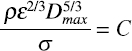
Empirical equations for droplet breakup stem from the theoretical arguments of Hinze (1955). He developed an expression for the maximum stable droplet size Dmax by assuming it would be small enough to lie within the inertial subrange of a turbulent flow, where the turbulent dynamics are isotropic and depend on the dissipation rate ε and kinematic viscosity ν of the turbulent, continuous phase. Because pressure fluctuations in the turbulent field generate the forces causing breakup, Dmax also should depend on the density ρ of the continuous phase. The forces resisting breakup are represented by the interfacial tension σ between the dispersed and continuous phases and on the dynamic viscosity μp and density ρp of the dispersed phase. Hinze (1955) arranged these parameters into a non-dimensional Weber number Wep and viscosity group (see Box 5.3). For the limiting case of a dispersed phase with low viscosity relative to interfacial tension, Hinze postulated the maximum stable droplet size would be given by a constant value of the Weber number group,
 |
(F.1) |
where C is an empirical constant. Hinze arrived at this form of We by recognizing that the dynamic pressure fluctuations in a turbulent flow scale as ρu′u′ and that it would be fluctuations on the scale of Dmax that would be responsible for breakup. Here, the prime indicates velocity fluctuations of the turbulence, and the overbar is an average in time. Within the inertial subrange, Batchelor (1951) had shown for isotropic turbulence that at a scale given by Dmax, then u′u′ = 2.0(εDmax)2/3.
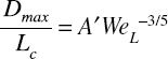
If we solve Equation F.1 for Dmax and then divide by a characteristic length scale Lc describing a given flow field, we obtain the general equation
 |
(F.2) |
where A′ is another empirical constant and WeL is the Weber number defined by length scale Lc, namely, WeL = ρε2/3L5/3/σ.
For the case where viscosity becomes an important resistive force relative to surface tension, Wang and Calabrese (1986) proposed a new viscosity number Vi based on experimental data in Calabrese et al. (1986) to replace Hinze’s original viscosity group. This new, non-dimensional group is given by
 |
(F.3) |
where U is a characteristic velocity scale of the turbulence. For the case of droplet breakup within the inertial subrange of the turbulence and following the same scaling arguments as in Hinze (1955) for the Weber number, the characteristic velocity scale would be U = (εDmax)1/3. Furthermore, it can be shown that any characteristic droplet size Dn can be related to Dmax by a numerical constant (Calabrese et al., 1986; Boxall et al., 2012). Here, Dn represents the droplet size for which n percent by volume of the other droplets in the flow are smaller than Dn; similar behavior holds for number size distributions. Hence, the breakup dynamics of an immiscible droplet in a statistically stationary turbulent field is generally described by
 |
(F.4) |
Equation F.4 is the basis for all empirical equations predicting characteristic droplet sizes of dispersions in turbulent flow, and the theoretical arguments underpinning this equation describe the dynamical processes responsible for droplet breakup: turbulent pressure fluctuations on the scale of a droplet and that scale with the dissipation rate ε break up a droplet until these forces can be resisted by the droplet interfacial tension and viscosity.
Empirical equations such as these predict one characteristic droplet size of the distribution. Hinze (1955) focused
on the maximum stable droplet size; other popular sizes are the volume median diameter, the size for which half of the volume is contained in smaller sizes, and the Sauter mean diameter, the size for with the surface area would represent that of the whole distribution if all droplets were of this size. To predict the whole distribution, this characteristic size should be related to an assumed probability density function. Common choices for the distribution of droplet sizes are the log-normal distribution and the Rosin–Rammler distribution, which are similar in their central tendency but differ in the shapes of their tales (Johansen et al., 2013; Wang et al., 2016, 2018; Li et al., 2017). Though some experimental studies show the width of fluid particle size distributions to be consistent across several experiments, Wang and Calabrese (1986) demonstrated that it depends on both the surface tension and viscosity of the dispersed phase through a resistance-to-breakup formulation. Falliettaz et al. (2021) also showed recently that even using the same median droplet sizes and distribution widths, the fate of oil in the water column and sea surface remained sensitive to the choice of analytical distribution when comparing Rosin–Rammler, log-normal, and one distribution from the viscous breakup model for oil droplets, VDROP. Hence, additional experiments and model calibration are required for empirical equations to predict the whole fluid particle size distribution.
F.2 APPLICATION OF TURBULENT BREAKUP FOR MULTIPHASE JETS
The equations and parameterizations in the previous section can be used to predict droplet sizes for different multiphase flows by relating the large-scale flow and turbulence production to the dissipation rate of turbulent kinetic energy at the small scales. Because turbulence is a property of the flow field, this yields a unique parameterization and different fit coefficients for different flow types. This section considers the case of breakup for turbulent jets, which resemble the flow from pipeline leaks or oil well blowouts, using both the empirical equations and population balance modeling approach to predict droplet sizes. Refer to Section 5.2.3.2 for more details, applications, and a discussion of available data for model validation.
Johansen et al. (2013) and Li et al. (2017) apply empirical equations to predict the characteristic droplet sizes for oil and gas jets. Johansen et al. (2013) handle the viscosity limitation on droplet formation using a modified Weber number that combines the normal Weber and viscosity numbers, similarly to that used by Johansen et al. (2015) for surface breaking waves. Li et al. (2016) follow the parameterization in Hinze (1955), using the Weber and Ohnesorge numbers. Johansen et al. (2013) take the turbulent eddy dissipation rate as that of the potential core in the zone-of-flow-establishment in turbulent jets, or the ZFE, of the jet release, ε = U03/D, together with the characteristic length scale LC = D to define the Weber and viscosity numbers. U0 is the jet exit velocity, and D is the jet orifice diameter. Li et al. (2017) take a different approach for the characteristic length scale, setting LC equal to the smaller of the orifice diameter D or the maximum stable droplet size d0, given by analytical stability analysis (Clift et al., 1978). Likewise, they assume ε = U03/LC so that there is only one length scale used to define the Weber number. When the orifice is small, the Weber numbers in Li et al. (2017) and in Johansen et al. (2013) would be the same. As the orifice diameter exceeds the maximum stable droplet size, the Li et al. (2017) model switches to a parameterization based on d0. Because the droplet size scales with the nozzle diameter for smaller nozzles, the Li et al. (2017) parameterization retains consistency in which the parameterization scales with droplet size despite the apparent discontinuity in switching from D to d0 as the nozzle size increases.
Both the Johansen et al. (2013) and Li et al. (2017) equations require calibration with data. Johansen et al. (2013) take the power-law relationships in their equations from the theoretical arguments in Hinze (1955) and Wang and Calabrese (1986), only fitting a coefficient multiplying the Weber and viscosity number to data measured in a series of experiments for oil jets into water. Brandvik et al. (2018) updated the fit coefficients to their current accepted values and summarized the complete datasets used to calibrate and validate the equation fit. Li et al. (2017) take both the power-law and proportionality constants as unknown. They fit the power-law relationship to experimental data for oil slick breakup under breaking waves and argue that these scaling laws should be universal. The fit coefficient multiplying the Weber and Ohnesorge numbers for jet breakup of oil are fitted to the field measurement from the DeepSpill experiment only (Johansen et al., 2003), thus having perfect agreement with these field data. They then validate the fit to other experiments in the laboratory, including those by Brandvik et al. (2013). In this way, both models are calibrated and validated to laboratory data for oil jets into water.
Other researchers have proposed alternative empirical equations to predict droplet size. The equations used by Paris et al. (2012) and Aman et al. (2015) use correlations from Boxall et al. (2012) to predict droplet sizes from the Deepwater Horizon (DWH) accident. Boxall et al. (2012) evaluated the effect of viscosity on droplet breakup by using different oils in the place of water as the continuous phase and observed the breakup of water droplets in a mixing tank using a Rushton-type, six-blade turbine. Mixing tanks are often used to evaluate oil and water emulsions because their turbulence characteristics have been well characterized and parameterized in terms of the blade diameter and rotation rate of the blades. Boxall et al. (2012) found both Weber number and Reynolds number scaling, where the viscosity of the continuous phase is used to define the Reynolds number. Because relatively inviscid water was the only dispersed phase used, they did not find a dependence on the viscosity number. However, they did demonstrate that for We4/5/Re > 0.1, droplet breakup continues below the Kolmogorov scale and
into the dissipation range of the turbulence. Although these physics and scaling laws likely are universal for droplet breakup in turbulent flows, the fit coefficients of Boxall et al. (2012) are only applicable to steady, constant turbulent dissipation rate, unlike that in a blowout jet, and should be used only for within-pipe flow where these turbulent conditions are present.
Zhao et al. (2014) used an experimentally derived expression for turbulent eddy dissipation rate in single-phase jets to adapt the VDROP population balance model to predict droplet evolution in subsea blowouts, yielding the jet-version of the model, VDROP-J. The original VDROP model solves for the unsteady evolution of the droplet size distribution under constant turbulent conditions of a mixing tank. The evolution of the turbulent eddy dissipation rate along the jet centerline was incorporated into the model following the classical Lagrangian integral model approach (Lee and Chu, 2003) in which a well-mixed control volume propagates along the jet centerline, advected at the mean jet velocity. Hence, the eddy dissipation rate variation with distance becomes a variation with time in the VDROP-J model. Coalescence was considered negligible, and the breakup parameter Kb, which sets the breakup efficiency, was calibrated to experiments on oil jets in water. A non-dimensional, universal calibration for Kb was not found; instead, the best-fit Kb depended on the initial dynamic momentum flux of the source. Zhao et al. (2015) apply the VDROP-J model to scenarios typical of the DWH accident. Zhao et al. (2016) adapt the model to bubble breakup, and Zhao et al. (2017) consider breakup of combined oil and gas releases. Predictions from VDROP-J for DWH were also used by Gros et al. (2017) to hindcast the fate of oil and gas released on June 8, 2010.
This page intentionally left blank.


