
8
Predictive Modeling
Corrosion is a process that, in theory, could be accurately predicted if sufficient information about the corrosion/infrastructure system is available. An engineering model, in general terms, is a simplified physical or mathematical representation of a system that can be used to predict system behavior and engineering performance, and can be used to influence engineering design. Models differ in complexity and scale, but they may be used to better understand how characteristics of the steel or subsurface will affect metal loss or inform choice of corrosion protection. The corrosion process is dependent on the details of the corroding interface including surface and environment composition and structure. Variations in these factors at the micrometer scale can have a controlling influence on corrosion and can also change with time. However, it is rarely possible to obtain sufficient information to accurately predict exactly when, where, or by what mechanism corrosion will occur. Ultimately, the goal in the field of the corrosion of buried steel structures is related to understanding the reliability of the structures. Community experts in structural reliability have developed methods to estimate the integrity and reliability of structures (e.g., Melchers and Beck, 2018). However, the effects of corrosion are generally not considered in detail (see Box 8.1).
The modeling approaches used by the geo-civil and oil and gas pipeline industries differ greatly, as do other aspects of engineering practice. The geo-civil industries tend to use models prior to design to predict metal loss with time and therefore to determine the additional steel necessary in design to compensate for that metal loss due. The oil and gas pipeline industries tend to emphasize modeling of the steel infrastructure during operations and maintenance, using data collected from indirect or in-line inspection (ILI) monitoring (see Chapter 7). Table 8.1 provides examples of current and evolving model types. The models are classified as deterministic and nondeterministic and are listed in order of increasing complexity and computational resources. Deterministic models are those that do not include randomness and will always produce the same output from given starting conditions. Nondeterministic models, in contrast, can exhibit different behaviors on different runs from the same starting conditions because these models consider different possibilities among the variations of input parameters (e.g., soil properties, initial zinc thickness, metal loss model parameters). Models used for geo-civil applications are generally deterministic and often involve empirical or semiempirical estimates of metal loss. These empirical and semiempirical approaches historically have dominated in corrosion engineering due to limited databases and computing power, but nondeterministic models may be better suited to situations that have a large number of variables and uncertainties. Only those conducting academic research and those in the oil and gas pipeline industry commonly use nondeterministic models.
While multiple model types are used in corrosion management practice, the most common, especially in the geo-civil industries, are empirical models. These models assume the same corrosion behavior at sites with similar characteristics and properties. Empirical models are most powerful when informed by laboratory and controlled field test data and combined with observations from in-service performance. However, in practice the data that form the basis for empirical models are limited in terms of breadth, quantity, and quality. Other types of models, including analytical, numerical, and statistical models, also may be used in practice, especially in the oil and gas industries. The next few sections describe models applied commonly in practice related to corrosion management. The final section of this chapter describes emerging trends in corrosion-related modeling.
EMPIRICAL MODELS FOR CORROSION RATE BASED ON SUBSURFACE PROPERTIES
One type of empirical model estimates corrosion rates based on subsurface characterization measurements (see Chapter 6). King (1977) described an American nomogram based on soil resistivity and pH that provides average corrosion rates for burial times of greater than 2 years. That nomogram can be used to predict rates of weight loss over time and corrosion due to pitting. Using corrosion data from field surveys, King checked the accuracy of the nomogram and found that the model was able to predict corrosion rates with ±10 percent accuracy for 30 percent of cases tested, but the remaining cases were accurate to only ±50 percent. He noted that the nomogram generally predicted lower corrosion rates than indicated by field measurements of corrosion, but corrosion rates in sandy soils predicted by the nomogram appeared slightly more reliable. This indicates that this nomogram provides only rough estimates of corrosion rates and is not dependable for use in design. Models similar to this nomogram have been produced by various state transportation agencies for galvanized steel and by NACE (2001). NACE modeled corrosion rates of steel piles above the water table correlating data from Romanoff (1957) and from seven other
TABLE 8.1 Types of Models Applied to Problems Related to Corrosion of Buried Steel
| Model Type | Definition | Typical Use | Example Outputs for Corrosion Applications | Example Inputs for Corrosion Applications |
|---|---|---|---|---|
| Deterministic Models | ||||
| Empirical | Directly relate input to a database of observations or experimental data | Research and the geo-civil industries | Corrosion rate | Measured soil resistivity and pH |
| Metal loss | Experimentally derived estimates describing corrosion rate in 1 year and a time constant describing change of corrosion rate over time | |||
| Semiempirical | Use simplified calculations to relate input to a database of observations or experimental results to obtain an answer | Academia and industry use | Metal loss due to galvanic corrosion | Difference in the respective corrosion potentials; kinetics of the electrochemical reactions on each metal, areas of each metal, and the ohmic resistance of the electrolyte to which they are exposed |
| Analytical | Mathematical models that describe an exact change in a system through solution of a mathematical analytic function | Used in research and rarely in oil and gas industries | Effectiveness of cathodic protection and the likelihood of corrosion | Measurements of a corrosion defect and of potential, current, and impedance profiles |
| Corrosion rate | Measured electrochemical potential at surface, measured or calculated thermodynamic and kinetic parameters | |||
| Numerical | Computation of a large number of mathematical equations to find an approximate solution | Used in research and rarely in oil and gas industries | Finite element modeling to predict corrosion anomalies for cathodic protection systems | |
| Predictions of galvanic corrosion for components with complex shapes | Electrical or thermal field given conductivity and appropriate boundary conditions | |||
| Nondeterministic Models | ||||
| Statistical | Mathematical model incorporating set of statistical assumptions about sampling of corrosion processes or corrosion damage | Used in research and in oil and gas industriesa | Probability of pipeline failure, uncertainty of corrosion rate, uncertainty of corrosion depth | Defect measurements |
| Stochastic | Mathematical model to estimate spatial/temporal variation of possible outcomes; variation usually based on historical data | Used in research and in oil and gas industriesb | Spatial distribution or occurrence of corrosion defects or events, temporal fluctuation of corrosion rate or current | Historical inspection data; soil survey results; climate, geological, and geotechnical data |
| Model Type | Definition | Typical Use | Example Outputs for Corrosion Applications | Example Inputs for Corrosion Applications |
|---|---|---|---|---|
| Machine learning: Supervised (artificial neural network, linear regression, support vector machine); Unsupervised (clustering) | Data-driven modeling paradigm for constructing machine learning algorithms | Used in research and emerging in oil and gas industriesc | Predicting corrosion depth and location with quantified uncertainty, estimating similarity of corrosion environments among different sites | Historical inspection data, soil survey results, domain knowledge, and engineering experiences |
a Examples include Aziz, 1956; Caleyo et al., 2007; Evans et al., 1933; Gong and Zhou, 2017a,b, 2018a,b; Greene and Fontana, 1959; Gumbel, 1954, 2004; Ji et al., 2017; Mears and Evans, 1935; Melchers, 2003, 2004, 2005a, 2008; Shibata, 1991, 1996; Shibata and Takeyama, 1976; Zhou et al., 2017.
b Examples include Bazán and Beck, 2013; Caleyo et al., 2009; Dann et al., 2015; Engelhardt et al., 1999; Hong, 1999; Kamrunnahar and Urquidi-Macdonald, 2010, 2011; Laycock et al., 1990; Maes et al., 2009; Martín et al., 2010; Melchers, 2010, 2015; Provan and Rodriguez, 1989; Rodriguez and Provan, 1989; Shibata, 2013; Shibata and Takeyama, 1977; Valor et al., 2007; Velázquez et al., 2009, 2010; Zhang and Zhou, 2015; Zhang et al., 2013; Zhou, 2010.
c Examples include Dann and Birkland, 2019; Kamrunnahar and Urquidi-Macdonald, 2006; Rosen and Silverman, 1992; H. Wang et al., 2015a,b,c, 2016, 2019, 2021; X. Wang et al., 2021; Wen et al., 2009; Yajima et al., 2014, 2015.
sites. NACE (2001) concluded that corrosion rate is a function of pH and resistivity (ρ), with lower resistivity and pH correlating with higher corrosion rates:
| Corrosion rate ∝ (pH*log (ρ))−1 | Equation 8.1 |
The same relationship does not hold true for galvanized reinforcements because both acidic and alkaline conditions result in elevated zinc corrosion rates (Pourbaix, 1974). The regression presented by NACE is based on limited data, and the correlation is not high. However, it is an example of a multivariate model that estimates corrosion rate based on subsurface properties.
EMPIRICAL MODELS FOR METAL LOSS (ROMANOFF MODELS)
Another type of empirical model is that which uses experimental datasets (e.g., Romanoff, 1957) to derive equations and calculate metal loss over a specific number of years. Romanoff (1957) concluded that buried steel corrosion rates attenuate with time, depending on the degree to which the soil is aerated, which, in turn, is dependent largely on drainage. He found this observation applied to general corrosion as well as localized corrosion from pitting. He observed an approximately linear relationship over timescales of 10 to 20 years after plotting the logarithm of maximum pit depths or weight loss (uniform loss of thickness) versus the logarithm of time, such that they conformed to
| P = k1tn1 | Equation 8.2 |
and
| X = k2tn2 | Equation 8.3 |
where P and X (both in micrometers) are the maximum pit depth and uniform loss of thickness, respectively, after time t (years); k1 and k2 (both in micrometers per year) are the maximum pit depth and loss of thickness after the first year, respectively; and n1 and n2 are exponents that are less than 1. The values of n1 and n2 are related
to the aeration of the soil, with well-aerated soils corresponding to lower values of n1 and n2. Well-aerated soils with an abundant supply of oxygen have a high scaling tendency—the oxidation and precipitation of iron as ferric hydroxide occurs close to the metal surface to produce a protective scale. The protective scale formed in this manner tends to decrease corrosion rates with time, and this is modeled using lower values of n1 and n2. In poorly aerated soils, the products of corrosion remain as ferrous ions with a lower oxidation state and tend to diffuse outward into the soil, offering little or no protection to the buried steel, such that the initial corrosion rates decrease slowly with respect to time, if at all. The formation of a protective scale and attenuation of corrosion rates may also be affected by the corrosivity of the soil. Even in a well-aerated soil, high concentrations of soluble salts may prevent precipitation of protective layers of corrosion products. The rate of corrosion would not decrease over time, and the corresponding value of the time constants would be closer to 1.
An iteration of the Romanoff model was presented by Darbin et al. (1988) and is applicable for galvanized steel in constructed earth fills. This study provides additional data from a 20-year study that evaluated the corrosion of galvanized steel elements in free-draining granular soils. This is important as fewer than 10 percent of the original Romanoff (1957) data come from free-draining granular soils such as those used in constructed earth applications, and not many include galvanized steel samples. Using these data, Darbin et al. (1988) proposed that metal loss of galvanized steel in free-draining fills could be described with a constant exponent “n2” equal to 0.65 and a coefficient of k2 equal to 25 μm/yr or 20 μm/yr when fills have laboratory-measured resistivities of 1,000–3,000 or >3,000 ohm-cm, respectively. The constants k2 and n2 correspond to an upper bound of corrosion data instead of a best fit. In this sense, there is an unquantified margin of safety inherent to the Darbin model (see Box 8.2). The Darbin model is used commonly in the geo-civil industries and forms the basis for metal loss modeling, calculation of the amount of steel needed to compensate for corrosion losses, and simplified forms that consider corrosion rates to be constants over specified time intervals. The accuracy of the model varies with respect to soil parameters, and considerable scatter exists between predictions and observation for higher corrosion rates. In general, the model is applied as an envelope to the data and is conservative. The model cannot be applied to the behavior of soils or metal types that were not included in the original database.
However, there are other mechanisms of corrosion than the uniform and pitting corrosion described by Equations 8.2 and 8.3 (see Chapter 4). The effects of other localized corrosion mechanisms are often incorporated into Equation 8.3 using a “correction factor,” also referred to as an “aggravation factor.” For example, Darbin et al. (1988) and Elias (1990) incorporated a factor of 2 to the steel corrosion rate after zinc is consumed (Equation 8.5) to account for macrocell corrosion processes in galvanized steel that may occur along with general corrosion. This is expressed as
| Equation 8.4 |
but
| Equation 8.5 |
where zi is the initial thickness of zinc coating (μm), X (μm) is the loss of base steel thickness after a certain number of years (t), k2 is the loss of thickness after the first year (μm/yr), and n2 is an exponent that is less than 1. This factor is strictly applicable to mechanically stabilized earth (MSE) wall reinforcements and is not necessarily applicable to describe the corrosion processes inherent to other systems.
A subsequent modification of this model was proposed by Bastick and Jailloux (1992) to describe how the corrosion of galvanized steel is affected by the salt content of fill. They demonstrated that the effects of chloride and sulfate species can be added together to render values of “k2” as a function of salt content such that
| Equation 8.6 |
where [Cl−] and [SO4] are the concentration of chloride and sulfate ions (ppm) in the fill.
In contrast to the above equations, other models approximate steel loss using a linear extrapolation of a constant steel corrosion rate that is multiplied by design life. One example is the American Association of State Highway and Transportation Officials (AASHTO) model that is specific to the design of galvanized reinforcements in MSE walls with noncorrosive or “mildly” corrosive fill.1 This model can be calculated as
| Equation 8.7 |
where X is the loss of metal thickness (µm), tf is the design life (years), C describes the time for zinc depletion, t1 is the duration for which the initial corrosion rate for zinc prevails (2 years for the AASHTO model), zi is the initial thickness of zinc, k2a is the initial corrosion rate of zinc for the time (t1), k2b is the subsequent corrosion
___________________
1 According to AASHTO, MSE fill must comply with the following electrochemical criteria: pH = 5 to 10, resistivity ≥3,000 ohm-cm, chlorides ≤100 ppm, sulfates ≤200 ppm, organic content ≤1 percent.
rate of zinc until exhaustion, and k2c is the corrosion rate of steel after zinc depletion. The AASHTO metal loss model defines values for “k2” at which first zinc, then steel, will be lost from the galvanized steel cross section:
| k2a: Loss of zinc during first 2 years (t1 = 2) | 15 µm/yr |
| k2b: Loss of zinc after first 2 years to depletion | 4 µm/yr |
| k2c: Loss of steel (after zinc depletion) | 12 µm/yr |
Both the AASHTO and Darbin et al. (1988) models compute the same metal loss with respect to a service life of 65 years. But for longer service lives (e.g., 75 or 100 years), the linearized AASHTO model renders more metal loss compared to the power law implemented for the Darbin model (Fishman and Withiam, 2011). The AASHTO model is the most popular metal loss model applied to the design of MSE reinforcements. However, this model should only be applied for fills that meet the limits and ranges of electrochemical parameters specified by AASHTO and is only applicable to galvanized steel.
Subsequent developments that have built off of Romanoff (1957) include those by Melchers and Petersen (2018) in which they reinterpreted the data presented by Romanoff (1957) and proposed a bimodal model for estimating corrosion rates and service life. That bimodal model considers the progression of corrosion and is useful for recognizing the effect of soil type on the time-dependant performance of buried steel.
ANALYTICAL AND NUMERICAL MODELING FOR GENERAL AND LOCALIZED FORMS OF CORROSION
The general corrosion rate of metals in the subsurface can be predicted using mixed potential theory if the kinetics of the anodic and cathodic reactions on the metal surface are known. Mixed potential theory is based on the notion that the rates of the anodic and cathodic reactions must be equal under open-circuit conditions (i.e., no electrical connection to another metal or measuring instrumentation) to uphold charge conservation. The anodic and cathodic electrochemical reaction kinetics are assumed to follow the well-accepted Tafel equation that relates the rate of the reaction to the electrochemical potential at the surface (see Chapter 4) or mass transport limitations. The corrosion potential and rate (current density) can then be determined from the point where the lines representing the kinetics for the two reactions intersect (see Figure 4.2). Thermodynamic (equilibrium potential) and kinetic (exchange current density and Tafel slope) parameters are required as parts of the Tafel equation. As described in Chapter 7, these parameters can be determined empirically, but commercially available software uses thermochemical principles to estimate them. One example of commercially available software is OLI Studio from OLI Systems, Inc. (Anderko et al., 2001). A comprehensive thermodynamic database is used to provide a detailed speciation of the local environment including ion activities, transport properties, and fractional surface coverage of adsorbed species, which then allows for determination of the required parameters in the Tafel equation using other models. The software also contains models for the prediction of passive oxide film formation and the stability of localized forms of corrosion such as pits and crevices.
Localized forms of corrosion can be modeled given advances in the understanding of the physicochemical process involved (Frankel et al., 2017; Li et al., 2018a,b, 2019a,b, 2021; Oldfield and Sutton, 1978). Models for pitting corrosion focus primarily on pit growth. The ability to predict initiation events is less developed. Galvanic corrosion (see Chapter 4) can also be modeled using this approach. Several factors will control the extent of the galvanic interaction: the difference in the respective corrosion potentials, the kinetics of the electrochemical reactions on each metal, the areas of each metal, and the resistance of the soil to which they are exposed. If these factors are known, then it is possible to accurately predict the extent of galvanic corrosion. Furthermore, it is possible to make predictions for components with complex shapes using finite-element approaches to solve the Laplace equation, which describes an electrical or thermal field given a conductivity and appropriate boundary conditions (Palani et al., 2014).
Commercially available software exists specifically for the prediction of galvanic corrosion. Some examples include CorrosionMaster (Elsyca, 2022), Galvanic Corrosion Simulator (BEASY, 2022), Corrosion Djinn (Corrdesa, 2022), and OLI Studio (OLI Systems, 2022). These software tools are used primarily in the research
community but are increasingly being used by infrastructure designers to predict corrosion rates and galvanic corrosion susceptibility. The U.S. Department of Defense has just approved a new standard practice (MIL-STD-889D, 2016) that “defines and classifies galvanic compatibility of electrically conductive materials and establishes requirements for protecting electrically conductive materials in a dissimilar couple against galvanic corrosion.” The standard replaces an older standard based only on corrosion potentials, which can result in incorrect recommendations. The new standard is based on polarization curves using predictions of the sort provided by the commercial software listed above. These programs require a reliable and robust database and struggle to predict variations in conditions over time, including the metal surface conditions and local electrolyte composition, which can have large effects on corrosion rate.
NUMERICAL MODELS FOR PREDICTING STRAY CURRENT
As described in Chapter 4, stray current is commonly produced by the electromagnetic inductance of a high-voltage alternating current power line, direct current (DC)-powered transit systems, or cathodically protected structures. Numerical modeling can be used to understand variables that affect the magnitude of the stray current (Finneran et al., 2015). For stray current produced from a power line, a transmission line model is used to calculate the propagation direction parallel to the electric field vector. The routing of the steel infrastructure and transmission line networks are incorporated into the numerical model colocations represented with connected finite sections and nodes. The model renders the potential, current, and current density for each colocation. For DC-powered transit systems, numerical models can be used to estimate how well the design of the transit system complies with allowable stray current (Flounders and Memon, 2020). Corrosion engineers can use those data to calculate the stray-current leakages and determine the level of track-to-earth resistance needed in the design. The utility of the software is limited by the accuracy of the input data. Often the uncertainty in critical input variables such as the current load, electrochemical properties of soils and fill, and the effects from transients (e.g., formation of scale from corrosion products) limits the benefits of a more complex model.
MODELING CATHODIC PROTECTION POTENTIAL AND CURRENT PROFILES, POLARIZATION, AND CURRENT DENSITY
Chapter 5 describes how buried steel forms a natural electrochemical system that can be altered to protect the buried steel by installing a cathodic protection (CP) system, and Chapter 7 describes how the CP effectiveness can be monitored. Modeling of the electrochemical processes in these systems is often useful both in design and during monitoring of the CP system. Before CP installation, modeling can help establish the current density necessary to properly protect the steel (typically in units of milliamperes per square foot). This current density may change due to the distance from the CP source and the local subsurface conditions (e.g., resistivity). Another parameter commonly modeled during design is the polarization of the buried steel infrastructure. Subsurface conditions can have a strong impact on polarization, which can change the overall effectiveness of the CP.
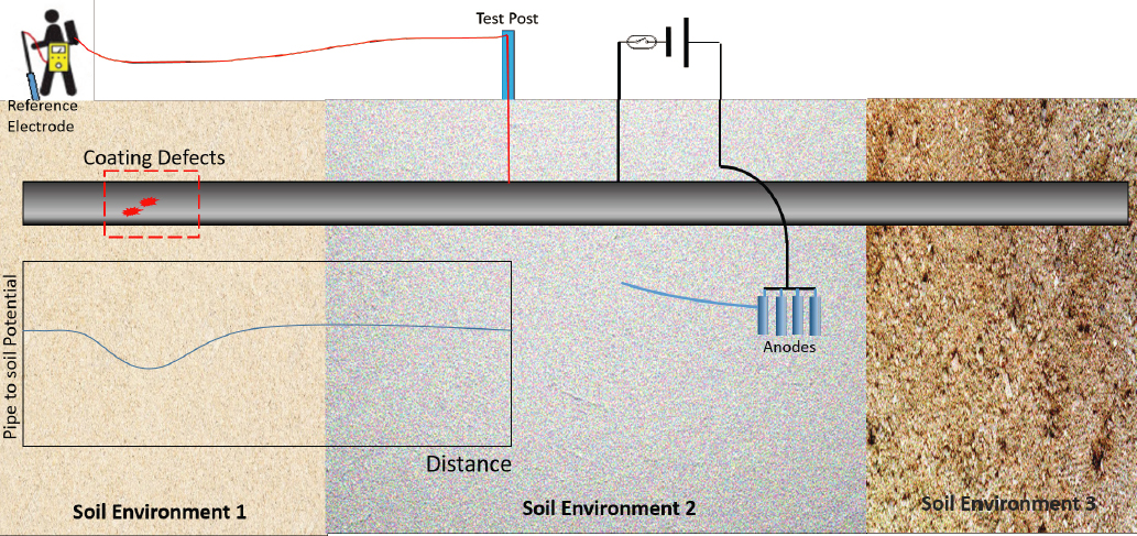
After installation of infrastructure, current and potential distribution models are commonly used to monitor cathodically protected steel. The distance from the CP source and the local conditions of the buried structure and subsurface often leads to different current distributions that are measured during monitoring with methods such as close interval potential surveys (CIPSs). Modeling the potential and current profile distribution locates the sites where the steel might not be protected (see Figure 8.1). Kennelley et al. (1993) and others have quantified potential and current distribution of CP-protected pipelines for several conditions, including inhomogeneous soil, with “holidays” or coating defects and with varying anode distribution. These data have been used reactively to adjust CP conditions and respond to corrosion concerns. Commercial software exists specifically for the prediction of CP characterization. Some examples are Comsol (Fontes and Nistad, 2019), Elsyca (2022), and BEASY (2022).
EMERGING AND EVOLVING TRENDS
Many of the emerging or evolving trends in corrosion modeling use probabilistic modeling and machine learning (ML) to calculate statistics instead of relying on factors of safety. However, these types of models often require larger datasets than are currently available. Other emerging trends attempt to use basic materials parameters on the atomic scale to produce models predicting the lifetime of macroscale steel infrastructure. The next sections describe aspects of these modeling techniques.
Probabilistic Modeling for Corrosion Rate and Severity
Recent efforts in corrosion science have attempted to try to implement probabilistic reliability-based models, instead of “go/no-go” models that are based on factors of safety. This has been more successful in recent years in the oil and gas pipeline industries that utilize ILI data from “smart pigs” to measure size, shape, and locations of defects (see Chapter 7). Models can help determine the corrosion rate and whether the defect should be repaired or replaced. One of the earliest and most practical probabilistic models in corrosion science is the burst prediction model (ASME B31G-2012 (R20170), 2017), which takes the measurements of a corrosion defect and determines if and at what pressure the pipe is likely to fail. However, this model does not truly model corrosion but rather models the pressure that can be sustained by a corroded pipe. Additionally, this model uses a factor of safety instead of true probabilistic modeling to determine failure probability. More complicated probabilistic analysis can categorize the severity of the corrosion and the rate of corrosion using multiple different ILI technologies and soil measurements (Yajima et al., 2015). Whereas the technologies utilized in ILI and subsurface characterization are standardized, the analysis and computer tools are not.
Another type of probabilistic model that can be applied to corrosion science is the application of extreme-value statistics, which use statistical approaches to focus on the tails of a distribution. Aziz (1956) was the first to recognize that the deepest pit in a distribution of corrosion pits will be the likely cause of an eventual failure, which led to the application of extreme-value statistics to model such data (Melchers, 2005b,c, 2008; Shibata, 1991, 1994). Asadi and Melchers (2017) applied extreme-value statistics to the corrosion of buried cast iron water pipes. The deepest pits were found to follow a Gumbel distribution, which is a mathematical function used to
describe the maximum values in a dataset. Another approach for predicting pitting corrosion is based on comparing the distributions of the corrosion (Ecorr), pitting (Epit), and repassivation (Erp) potentials. One study (Cong and Scully, 2010) concluded that “pitting can occur once the maximum [open-circuit potential] rises up to within three standard deviations of Epit (99.7 percent) and exceeds Erp.”
Machine Learning
Few large and comprehensive datasets exist in corrosion science and corrosion engineering. The Romanoff (1957) data are limited in scope, which reduces the predictive ability of any analysis of his data. However, if a sufficiently large dataset were available (e.g., on the order of thousands of data points), then sophisticated new analysis methods could be applied. In recent years, approaches that simulate human thinking—known generically as artificial intelligence—have been applied in numerous fields such as handwriting and speech recognition, marketing, economics, robot locomotion, and search engines. ML is a subset of artificial intelligence that uses computer algorithms to seek and analyze trends and patterns in datasets and create predictive relationships or assign categories. ML approaches are classified as either supervised or unsupervised. Supervised learning uses a training sample set with predetermined outputs to build a model capable of predicting the output of unknown samples. In contrast, unsupervised learning uses a training set without preassigned outputs or labels with the goal of allowing the algorithm to find patterns and clustering. Effective ML requires large, high-fidelity datasets to allow accurate training as well as validation and testing of the algorithms.
The oil and gas pipeline industries have generated large volumes of data as a result of regulatory requirements for active integrity programs and the ability to collect pipe corrosion data using sensors in smart pigs. Those data combined with the need to maintain the integrity of hundreds of thousands of miles of pipeline have stimulated the use of ML in the pipeline industry. Pipeline operators must assess the risks and consequences of failure (e.g., as a result of a leak). Recent papers have summarized the use of ML in pipeline integrity management (Ossai, 2020; Rachman et al., 2021; Soomro et al., 2022) as well as for the detection of defects in inspection data (Rachman et al., 2021).
Different ML methods exist, some of which are available as simple laptop-based software or libraries (Paszke et al., 2019; Pedregosa et al., 2011). A common approach, artificial neural network (ANN) analysis, attempts to mimic the behavior of the human brain, which is skillful at sensing patterns (Bishop and Nasrabadi, 2006). ANN utilizes a connected array of nodes, similar to neurons, including input nodes (data descriptors), output nodes (desired predictions), and intermediate hidden nodes that connect them. Mathematical expressions form the connections between the nodes. ANNs have been applied to corrosion data in recent years. For example, Birbilis et al. (2011) used ANN to model the effects of composition on corrosion rate and strength of 68 different magnesium alloys. The model predicts the properties of untested alloys, possibly accelerating the development of new alloys with improved properties. Neural networks have also been used to assess images of steel structures to determine, by ML only, if they were corroded (Atha and Jahanshahi, 2018). Almost 70,000 images of both corroded and noncorroded regions were used for training, validation, and testing. The precision was found to be greater than 90 percent.
Other ML methods employ decision-tree analysis and regression approaches such as ordinary linear regression (Weisberg, 2005), ridge regression (Arashi et al., 2019), kernel regression, and logistic regression (which is commonly used in biostatistics to sort out the efficacy of drugs or other medical treatments; Johnell and Klarin, 2007). Bayesian networks are useful for capturing the knowledge of human experts and the rules they use for relating causes and outcomes (Heckerman, 2008). This approach of knowledge-based analytics is particularly useful in areas—such as corrosion—where data are often scarce but experts have deep understanding. ML can also integrate stochastic models with explicit consideration of uncertainty, which is suitable for complex heterogeneous soil distribution environment (H. Wang et al., 2015a,b, 2016, 2019, 2021; X. Wang et al., 2021; Yajima et al., 2015). It has become a tool used in the pipeline industry to characterize and quantify damage, risk, and integrity (Kim et al., 2021).
Whereas the oil and gas pipeline industries have generated large volumes of data and have applied ML techniques, those databases are often proprietary, or their use is restricted for homeland security reasons. ML could be applied more commonly to predict corrosion of buried steel in geo-civil infrastructure given a sufficient dataset
representing corrosion rates of buried steel over a range of conditions and including a variety of soil types, groundwater levels, moisture contents, resistivities, pH, and chloride and sulfate concentrations.
Atomistic Modeling and Density Functional Theory
Fundamental first-principles modeling of corrosion has been a focus of research in recent years. One approach, known as density functional theory, solves an equation similar to the Schrodinger equation for a small cluster of atoms to determine factors such as the electron density distribution, system potential energy, band structure, and the equilibrium atomic structure. These parameters can be used for a variety of fundamental applications relevant to corrosion, such as assessing chemical bond strength, reaction mechanisms, activation energies and reaction kinetics, and mechanical properties (Ke and Taylor, 2019). These are basic materials parameters, which would need to be fed into larger-scale models to arrive at practical predictive models of corrosion. The goal is a multiscale model that starts with electronic configuration and ends up with a prediction of a component lifetime. Practical application of atomistic modeling will not be achieved without considerable resources and time.


