
Appendix G
Data Analysis Report
DATA ANALYSIS REPORT
Data Analysis for the Committee to Review the DRIs for Energy
October 19, 2022
Indiana University, School of Public Health – Bloomington
Dean David Allison, Dean and Distinguished Professor, Provost Professor, Department of Epidemiology & Biostatistics
Dr. Carmen Tekwe, Associate Professor, Department of Epidemiology & Biostatistics
Dr. Roger Zoh, Associate Professor, Department of Epidemiology & Biostatistics
Stephanie Dickinson, Executive Director, Biostatistics Consulting Center
Lilian Golzarri Arroyo, Biostatistician II, Biostatistics Consulting Center
Aaron Cohen, Biostatistician I, Biostatistics Consulting Center
Jocelyn Mineo, Research Associate, Biostatistics Consulting Center
1. INTRODUCTION
1.1 Introduction and Summary of Work
The team at Indiana University (IU), School of Public Health-Bloomington, was engaged to perform statistical analysis to derive equations for the estimation of energy expenditure in the general human population, including pregnant and lactating women in the USA and Canada, based on data collected across multiple studies using the doubly labeled water (DLW) method for measuring Total Energy Expenditure (TEE) under free-living conditions.
Four primary sources of data were sought:
- Institute of Medicine (IOM)’s 2002/2005 Report1 for Dietary Reference Intakes (DRIs) for Macronutrients,
- International Atomic Energy Agency (IAEA),
- Study of Latinos: Nutrition and Physical Activity Assessment Study (SOLNAS) data from the National Heart, Lung and Blood Institute (NHLBI) Biologic Specimen and Data Repository,
- Harvard Men’s Lifestyle Study.
Data were obtained from IOM, IAEA, and SOLNAS as described below; however, data were not obtained from Harvard Men’s Lifestyle Study in time for inclusion in this report. An additional data source was added for pregnancy data from the Children’s Nutrition Research Center (CNRC) to increase the sample sizes for pregnant and lactating women.
The first task was to request data from the relevant sources, preparing Data Use Agreements (DUAs) as needed, including lists of the specific variables requested, including TEE, Basal Energy Expenditure (BEE; or basal metabolic rate [BMR]), age, sex, height, weight, body composition, physical activity, health status, athletic status, and country codes. The IU team then worked diligently to harmonize variable names, recode classifications, and combine these across data sets, resulting in 8,600 observations (cases) in the pooled data set.
Multiple tables of descriptive statistics and visualizations were provided for each dataset to allow Workgroup 1 (WG1) of the DRI energy committee to thoroughly inspect the data.
One challenge for the IU team was to consider how to perform predictive modeling of TEE based on physical activity level (PAL) while PAL (=TEE/BEE) was missing for 54.2% of the data (4,662 out of 8,600) where BEE was unavailable. Multiple Imputation was selected as the best method to impute the data rather than simple estimates of BEE (or more
___________________
1 IOM (Institute of Medicine). 2002/2005. Dietary Reference Intakes for energy, carbohydrate, fiber, fat, fatty acids, cholesterol, protein, and amino acids. Washington, DC: The National Academies Press.
accurately, BMR) based on age, sex, and weight in equations such as that published by Schofield2 or others.
Additional work between IU and WG1 involved physical activity data and to consider how PAL should be included in predictive equations of TEE. Initial models used the same cutoff criteria and model forms used in the 2002/2005 IOM report, but methods were revised to use different PAL criteria, which vary by age groups per discussion with WG1, as described below.
Prediction equations were then developed by fitting linear models on TEE based on sex, age, PAL, weight, height, and body composition. Multiple imputation was used to estimate PAL across 20 versions of imputed data, where models were fit to each of the 20 imputations, and the results were pooled to identify final parameter estimates and standard errors (SEs) as defined by Rubin.3
Models were fit for the overall sample and were then separated by including different Body Mass Index (BMI [kg/height or length]2) groups: BMI 18.5 to 40 (removing extremes); BMI 18.5 to 25 (“healthy” only); and BMI 25+ (overweight/obese only) to compare how regression slopes may differ by weight status groups.
The prediction of TEE with models using height and weight were also compared to those with height, fat-free mass (FFM), and fat mass (FM).
Models were fit separately in 7 strata:
- Infant/Toddler Boys (0–2.99 years old),
- Infant/Toddler Girls (0–2.99 years old),
- Boys (3.0–18.99 years old),
- Girls (3.0–18.99 years old),
- Men (19 and over),
- Women (19 and over),
- Pregnant
Model validation was performed on the external data (described below) provided by WG1 as summary data extracted from the literature. Parameter estimates from the TEE equations developed on the main data set were used to calculate predicted values of TEE on the external data, and those predicted values were compared to the observed TEE values using measures such as R-squared and correlation as a measure of model fit and performance.
2. IAEA DATA PREPARATION
IAEA data were obtained by submitting an application to the database manager (Dr. John Speakman) for the IAEA’s doubly labelled water
___________________
2 Schofield, W. N. 1985. Predicting basal metabolic rate, new standards and review of previous work. Hum Nutr Clin Nutr 39(Suppl 1):5-41.
3 Rubin, D. B. 1987. Multiple imputation for nonresponse in surveys. New York: John Wiley & Sons.
database (https://doubly-labelled-water-database.iaea.org/). After the proper procedures and approval process from the database manager group, the data were transferred to Dr. Allison and his team in an Excel file “IAEA DLW database 3.6.1 abbreviated for DRI group (allison).xlsx”.
Additional documents used for the data preparation of the IAEA data:
- “IAEA publications description IU 060722 - LGA notes.xlsx”—A list of studies to include or remove as indicated by WG1
- “CLASS 2022-06-13.xlsx”—Categories of Income by Country to indicate high-income countries for inclusion, provided by WG1
- Growth charts downloaded from https://www.cdc.gov/growthcharts/index.htm:
- Weightolength_WHO.xlsx”—Percentiles for weight-for-length for infants (0–2) per World Health Organization (WHO)
- BMIcharts.xlsx”—BMI percentiles for children (2–18) per Centers for Disease Control and Prevention (CDC)
The first step in preparation of the data was to apply the exclusion/inclusion criteria defined by WG1:
- The International Organization for Standardization (ISO) codes found in the “CLASS 2022-06-13.xlsx” file were used to exclude all studies being done in non-high-income countries.
- The codes under the column “Health” in the DLW database were used to include subjects who were healthy, labeled as H. Subjects with a code beginning with a D, such as D1 or D15 were excluded.
- Professional athletes were removed from the data set by excluding those listed as PA in the ‘ath’ column.
- Ineligible studies were removed according to the Excel file “IAEA publications description IU 060722,” which WG1 highlighted yellow or indicated in workgroup meetings, for which IU coded as “1” in the Excel file in a column “Remove” to remove via SAS code. Those coded as “2” indicated special cases, which were inspected manually to exclude low-income countries or non-healthy participants.
After ineligible studies were removed, pregnant and lactating females were identified in order to be analyzed separately from other females in the study and coded for trimester and number of weeks of gestation or in the postpartum period, as follows:
Reproductive Status for Females (rep_statF)
- L=Lactating
- P1=Pregnant, 1st trimester (This did not exist in IAEA data after preparation steps above.)
- P2=Pregnant, 2nd trimester
- P3=Pregnant, 3rd trimester
Next, while fat mass percentage (FM_pct) was provided in the IAEA data, fat mass (FM) was calculated as:
FM=(FM_pct/100*FFM)/(1-FM_pct/100).
TABLE 1 Inclusion and Exclusion Criteria and Sample Size for the IAEA Data Set
| IAEA Inclusion/Exclusion | N |
|---|---|
| Read in the data | 7,696 |
| Only keep High-Income Countries | 6,989 |
| Remove any subject with a Health Code beginning with D | 6,744 |
| Remove Professional Athletes (PA) from PA category | 6,706 |
| Remove other ineligible studies | 5,966 |
| Remove those without age or sex | 5,805 |
| Remove participants with PAL < 1 or > 2.5 as defined in section 6.3. | 5,717 |
Based on the above, two analysis-ready data files were created:
- one including the 5,805 participants for preliminary descriptive statistics and visualizations before PAL exclusions (“IAEA”), and
- one with the 5,717 for final analysis (“IAEA_clean”).
3. IOM DATA PREPARATION
IOM data were obtained by extracting data from the pdf versions of the data listed in the appendix of the IOM’s 2005 publication6 and then converting into Excel.
___________________
4 Most, J., A. D. Altazan, M. St Amant, R. A. Beyl, E. Ravussin, and L. M. Redman. 2020. Increased energy intake after pregnancy determines postpartum weight retention in women with obesity. Journal of Clinical Endocrinology and Metabolism 105(4):e1601-1611.
5 Matsiko, E., P. J. M. Hulshof, L. van der Velde, M. F. Kenkhuis, L. Tuyisenge, and A. Melse-Boonstra. 2020. Comparing saliva and urine samples for measuring breast milk intake with the 2H oxide dose-to-mother technique among children 2-4 months old. British Journal of Nutrition 123(2):232-240.
6 Institute of Medicine. 2005. Dietary Reference Intakes for energy, carbohydrate, fiber, fat, fatty acids, cholesterol, protein, and amino acids. Washington, DC: The National Academies Press. https://doi.org/10.17226/10490.
The following data sets were read in for IOM data:
- “IOM2005_AppendixI_Tables_JM_LGA.xlsx” extracted from “IOM.2005.DRIs for Macronutrients.pdf”
- TABLE I-1 Infants and Very Young Children (0 Through 2 Years of Age) Within the 3rd to 97th Percentile for Body Mass Index (BMI)
- TABLE I-2 Normal Weight Children, 3 Through 18 Years of Age with Body Mass Index (BMI) > 85th Percentile
- TABLE I-3 Normal Weight Adults with Body Mass Index (BMI) from 18.5 up to 25 kg/m2
- TABLE I-4 Pregnant Women with Prepregnancy Body Mass Index (BMI) from 18.5 up to 25 kg/m2
- TABLE I-5 Lactating Women with Prepregnancy Body Mass Index (BMI) from 18.5 up to 25 kg/m2
- TABLE I-6 Overweight/Obese Children, 3 Through 18 Years of Age, with Body Mass Index (BMI) > 85th Percentile
- TABLE I-7 Overweight/Obese Adults with Body Mass Index (BMI) > 25 kg/m2
Gestation weeks in IOM Table I-4 were grouped into trimester (P_ stage), and lactation months in I-5 were grouped into 1–3 and 4–6 months postpartum.
TABLE 2 Inclusion and Exclusion Criteria and Sample Size for the IOM Data Set
| IOM Inclusion/Exclusion | N |
|---|---|
| Read in Table I-1 | 320 |
| Read in Table I-2 | 525 |
| Read in Table I-3 | 407 |
| Read in Table I-4 | 22 |
| Read in Table I-5 | 35 |
| Read in Table I-6 | 319 |
| Read in Table I-7 | 360 |
| Additional Combined Pregnancy Lactation Data | 382 |
| Merge all tables together | 2313 |
| Remove participants with PAL < 1 or > 2.5 as defined in section 6.3 | 2283 |
Based on the above, two analysis-ready data files were created:
- one including the 2,313 participants for preliminary descriptive statistics and visualizations before PAL exclusions (“IOM”), and
- one including the 2,283 for final analysis (“IOM_clean”).
4. CNRC DATA PREPARATION
The following data set was provided by WG1 and read in for the Children’s Nutrition Research Center at Baylor College of Medicine (CNRC):
- “CNRC Pregnancy w weeks 2022-08-20.xlsx”
Data include the number of weeks pregnant and weeks of lactation postpartum. Non-pregnant and non-lactating (NPNL) are also included, which were coded as weeks=0 for analysis.
The data set included 222 observations across 60 women (with three or four time points per women at preconception, second and third trimesters and six months postpartum)
TABLE 3 Inclusion and Exclusion Criteria and Sample Size for the CNRC Data Set
| CNRC Inclusion/Exclusion | N |
|---|---|
| Source data from CNRC | 222 |
| Remove participants with PAL < 1 or > 2.5 as defined in section 6.3 | 220 |
Based on the above, two analysis-ready data files were created:
- one including the 222 participants for preliminary descriptive statistics and visualizations before PAL exclusions (“CNRC”), and
- one including the 220 for final analysis (“CNRC_clean”).
5. SOLNAS DATA PREPARATION
DLW and physical activity data were obtained for Hispanic adults (19+) from The Study of Latinos: Nutrition & Physical Activity Assessment Study (SOLNAS) from the National Heart, Lung, and Blood Institute (NHLBI) BioLINCC site (https://biolincc.nhlbi.nih.gov/studies/hchssol/).
The following SAS data sets were read in for SOLNAS data:
- mysolnas.dlwa_lad1.sas7bdat
- mysolnas.vsea_lad1.sas7bdat
- mysolnas.biea_lad1.sas7bdat
- mysolnas.csea_lad1.sas7bdat
For the DLW data set (DLWA), only urine data were kept for TEE. The following variables were renamed according to the SOLNAS codebook.
TEE = DLWA33
BMI = DLWA34
FFM = DLWA35
FM = DLWA36
FM_pct = DLWA37
Height and weight were obtained from the main study visit 1 and visit 3 forms (VSEA) data set, and renamed as follows:
Height = VSEA3A
Weight = VSEA3B
For the body image (BIEA) data, data were only kept from the main study for gender, and the following variables were defined according to the codebook:
For the calorimetry summary (CSEA) data, data were kept from the main study for age and calorimeter weight, and the following variables were renamed:
Weight_calorim = CSEA2
Age = CSEA3
EE_mean_kcald= CSEA4D1
EE_SD_kcald= CSEA4D2
EE_CV_kcald= CSEA4D3
The variable ‘EE_mean_kcald’ was relabeled as ‘BEE.’
The ethnicity for all participants in this study was coded as ‘Hispanic,’ and none of the participants were pregnant or lactating.
Physical activity data were also explored where 69 subjects had physical activity data from Actical. We used the “Actical derived variables at the participant level” data set for minutes per day of sedentary, light, moderate, and vigorous activity to correlate with PAL from DLW data.
TABLE 4 Inclusion and Exclusion Criteria and Sample Size for the SOLNAS Data Set
| SOLNAS Inclusion/Exclusion | N |
|---|---|
| Merge data sets for DLW, VSEA, BIEA, CSEA | 393 |
| Remove those without age or sex | 382 |
| Remove participants with PAL < 1 or > 2.5 as defined in section 6.3 | 380 |
Based on the above, two analysis-ready data files were created:
- one including the 382 participants for preliminary descriptive statistics and visualizations before PAL exclusions (“SOLNAS”), and
- one including the 380 for final analysis (“SOLNAS_clean”).
6. COMBINED DATA
The data sets from IAEA, IOM, SOLNAS, and CNRC pregnancy were harmonized to use consistent variable names and then combined. Variables are described in Appendix N: DLW Data Codebook.
SID, Age_cat, Age, Life_Stage, Ethnicity, Sex, BMI, BMIcat, Height, Weight, TEE, BEE, Percentile, Percentile_group, Percentile_infant, Lactating, Pregnant, P_stage, Weeks, PAL, PALCAT, BMR_kcal_Schofield, PAL_est, PALCAT_est, FFM, FM, FM_pct.
The combined data set included 8,722 participants for preliminary descriptive statistics and visualizations before PAL exclusions and 8,600 observations after removing participants with PAL < 1 or > 2.5 as defined in section 6.3.
Data coding and preparations were performed as follows:
6.1 Age Categories
Age categories were defined as follows for descriptive statistics reports, according to “Life Stage” as indicated by WG1:
- Infants are 0 to 11.99 months
- Children are 12.0 months to 8.99 years
- Teenagers are 9.0 to 18.99 years
- Adults are 19.0 years to 101 years
However, the following age categories were used for strata for the final TEE models:
- Infants are 0 to 2.99 years
- Children are 3.0 to 18.99 years
- Adults are 19.0 years and above
6.2 PAL Categories
The IOM 2005 report previously classified people into physical activity categories using roughly 25th, 50th, and 75th quartiles of PAL values uniformly across all age groups:
If 1.0=<PAL<1.4 then PALCAT=Sedentary7
If 1.4=<PAL<1.6 then PALCAT=Low Active
If 1.6=<PAL<1.9 then PALCAT=Active
If 1.9=<PAL<2.5 then PALCAT=Very Active
Here, we used the same quartiles (25th, 50th, 75th) to group people into the four categories, where the workgroup decided to calculate quartiles separately within age groups: 3 to 8.99 years, 9 to 13.99 years, and 14 to 18.99 years. For adults, PAL categories were defined by the quartiles for 19 to 70 years, but these PAL categories were applied to all adults, including those aged 71 and greater.
PAL percentiles as calculated on the raw data (before imputation) are shown in Appendix P §4.10 as well as after multiple imputation as shown in Appendix Q §2.1 and also in results section below.
After inspecting the PAL percentiles by age groups (shown below), PAL categories were defined by WG1 accordingly, and categories (PALCAT) were calculated in the SAS code as follows:
___________________
7 Note that the term “Sedentary” and PALCAT=”S” is used in this report as well as the analytic code and output, according to the labels in the 2005 IOM report before the committee relabeled the lowest level as “inactive.”
>6.3 Data Screening
Because a PAL > 2.5 is considered unsustainable, participants with PAL > 2.5 were removed from analysis. A PAL < 1 is considered unphysiological, as it’s not possible for BEE to be larger than TEE. Where data
for BEE and PAL were missing, BEE and TEE were estimated using the Schofield equations8 for the purpose of data screening.
The SAS code for calculating BMR according to Schofield equations is as follows:
___________________
8 Schofield, W. N. 1985. Predicting basal metabolic rate, new standards and review of previous work. Hum Nutr Clin Nutr 39(Suppl 1):5-41. PMID: 4044297.
The following decision criteria were used to screen high or low values of PAL:
Note that while BEE and PAL estimates from Schofield were not used in TEE models, they were retained in the data set during multiple imputation as a “proxy” (or “auxiliary variables”) that correlated with the variable to be imputed, which improves the precision of estimates.9,10
TABLE 5 Sample Sizes for Final Analysis Data Set, after Exclusions, by Data Source
| Data source | N |
|---|---|
| IAEA | 5717 |
| IOM | 2283 |
| CNRC | 220 |
| SOLNAS | 380 |
| Combined data for analysis | 8600 |
___________________
9 Ejima, K., R. Zoh, C. Tekwe, D. Allison, and A. Brown. 2020. What proportion of planned missing data is allowed for unbiased estimates of the association between energy intake and body weight using multiple imputation? Curr Dev Nutr 4(Suppl 2):1167. doi: 10.1093/cdn/nzaa056_014. PMCID: PMC7258036.
10 Cornish, R. P., J. Macleod, J. R. Carpenter, et al. 2017. Multiple imputation using linked proxy outcome data resulted in important bias reduction and efficiency gains: a simulation study. Emerg Themes Epidemiol 14(14). https://doi.org/10.1186/s12982-017-0068-0.
Based on the above, two analysis-ready data files were created:
- one including the 8,722 participants for preliminary descriptive statistics and visualizations before PAL exclusions (“ALLDATA”), and
- one including the 8,600 for final analysis (“ALLDATA_clean”).
7. STATISTICAL METHODS
7.1 Multiple Imputation
PAL is a predictor in the TEE equations but was missing for 54.2% of the data (4,662 out of 8,600). Others in the field have estimated PAL using BEE (or actually, BMR) as estimated by equations such as Schofield (1985)11 based on age, height, and weight. However, Dr. David Allison and the IU team preferred to use multiple imputation (MI) to estimate a variety of possible values of PAL using the information available in the other variables and maintaining the variability of the true data.
Note that PAL estimates from Schofield were retained in the data set during multiple imputation as a “proxy” (or “auxiliary variables”) that correlated with the variable to be imputed, which improved the precision of estimates.12,13,14
The SAS procedure ‘Proc MI’ was used for imputation with Markov Chain Monte Carlo (MCMC) methods with multiple chains, using 20 imputations.
The combined clean data set (n = 8,600), including all ages and weights and pregnant and lactating women, was entered into the procedure with
___________________
11 Ejima, K., R. Zoh, C. Tekwe, D. Allison, and A. Brown. 2020. What proportion of planned missing data is allowed for unbiased estimates of the association between energy intake and body weight using multiple imputation? Curr Dev Nutr 4(Suppl 2):1167. doi: 10.1093/cdn/nzaa056_014. PMCID: PMC7258036.
12 Schofield, W. N. 1985. Predicting basal metabolic rate, new standards and review of previous work. Hum Nutr Clin Nutr 39(Suppl 1):5-41.
13 Cornish, R. P., J. Macleod, J. R. Carpenter et al. 2017. Multiple imputation using linked proxy outcome data resulted in important bias reduction and efficiency gains: a simulation study. Emerg Themes Epidemiol 14(4).
14 Li, P., and E. A. Stuart. 2019. Best (but oft-forgotten) practices: Missing data methods in randomized controlled nutrition trials. Am J Clin Nutr 109(3):504-508. doi: 10.1093/ajcn/nqy271. PMID: 30793174; PMCID: PMC6408317. https://www.ncbi.nlm.nih.gov/pmc/articles/PMC6408317/.
all variables in the data set. All missing data for all variables in the data set were simultaneously imputed (e.g. PAL, FM, FFM) providing 20 versions of a complete data set.
PAL data were then evaluated again in the imputed data for unrealistic values, where PAL values < 1.0 (unphysiological) were truncated (Winsorized) at 1.0, and observations with values > 2.5 (unsustainable) were removed from that version of imputed data before analysis. Because there were 20 imputed data sets, these values were only removed in that specific imputation, and that person would remain in the other imputations where the values remained < 2.5.
7.2 Statistical Modeling
TEE models were fit separately for each strata:
- Infant/Toddler Boys (0–2.99 years old),
- Infant/Toddler Girls (0–2.99 years old),
- Child/Teen Boys (3.0–18.99 years old),
- Child/Teen Girls (3.0–18.99 years old),
- Men (19 and over),
- Women (19 and over),
- Pregnant Women
Within each stratum, the linear models were fit separately on each version of the imputed data set, obtaining the relevant regression equations in each iteration.
TEE is estimated as a function of a person’s age, height and weight, and PAL, as a categorical measure “PALCAT”: Sedentary/Inactive, Low Active, Active, Very Active as described above based on PAL (=TEE/BEE). Interaction terms are used to fit separate slopes for the effect of height and weight within each PALCAT.
Because the raw parameter estimates for the model with interactions are not easily interpretable to a non-statistical audience, the IU team used ‘estimate’ statements in SAS15,16 to calculate the estimates (and Standard Errors) for slopes of weight and height within each PALCAT.
___________________
15 SAS Institute Inc. 2013. SAS/STAT 13.1 User’s Guide. Cary, NC: SAS Institute Inc., page 3459. https://support.sas.com/documentation/onlinedoc/stat/131/glm.pdf
16 Introduction to SAS. UCLA: Statistical Consulting Group, from https://stats.oarc.ucla.edu/sas/faq/how-do-i-write-an-estimate-statement-in-proc-glm/
The SAS code is pasted here, where &agecat. is a macro variable representing each age/sex strata. Also note that when reading the code below, the levels of PALCAT occur in alphabetical order in SAS (Active, Low Active, Sedentary, Very Active).
Coefficients obtained from the ‘estimate’ statements can then be presented more simply, to display an equation within each PAL category as:
where ‘A’, ‘B’, and ‘C’ are the model-based coefficients for slopes of Age, Height, and Weight, respectively, for each PAL category.
Parameter estimates are then pooled across the 20 imputations using ‘proc mianalyze’ in SAS to provide final parameter estimates and standard errors.
SAS code is pasted here, where &agecat. is a macro variable representing each age/sex strata.
Children 0 to < 3 years old did not have separate models by PAL category; all data were pooled.
Analysis of pregnancy data included longitudinal data for women by trimester. Non-pregnant and non-lactating (NPNL) were included, coded as weeks=0 for analysis. Linear mixed models were performed with Proc Mixed in SAS using a repeated statement to account for the correlation of data over time within women. A variable was also added to the model for weeks of pregnancy.
7.3 Model Performance and Evaluation
Model performance is calculated as:
- R2
- Adjusted R2
- Shrunken R2 (Browne formula)17
- Pearson r correlation
- MAPE (Mean Absolute Percentage Error)
- MAE (Mean Absolute Error)
- Mean squared error (MSE)
- Root mean squared error (RMSE)
using the following equations18:
___________________
17 Yin, P., and X. Fan. 2001. Estimating R2 shrinkage in multiple regression: A comparison of different analytical methods. J Experiment Educ 69(2), 203–224. http://www.jstor.org/stable/20152659.
18 Tibshirani, R., T. Hastie, G. James, and D. Witten. 2021. An introduction to statistical learning: With applications in R. United States: Springer US.
Let y1,…,yn be the observed values and ![]() be the predicted values; let the mean of the observed values be ; the mean of the predicted values be
be the predicted values; let the mean of the observed values be ; the mean of the predicted values be ![]() ; the residual sum of square be SSres = Σ(ŷ1 – ŷ1)2 and the total sum of squares be . Finally, let k be the number of predictors in the model. Then,
; the residual sum of square be SSres = Σ(ŷ1 – ŷ1)2 and the total sum of squares be . Finally, let k be the number of predictors in the model. Then,
These are calculated in R code as follows, where ‘TEE’ is the true observed data (yi), and ‘TEE_pred.o’ is the predicted value for TEE (ŷi). In the code below, the ‘o’ in TEE_pred.o is for the overweight/obese model, and the same is done for each BMI classification.
Note that both the RMSE and MAE are in the same units as the original TEE (kcal/day).
7.4 Model Validation
An out-of-sample model validation was performed on an external data set provided by WG1 (“Data extraction combined FINAL 081122”), which contained summary data (Means and SD) of DLW studies extracted from the literature and not in the combined DLW database.
Parameter estimates from the TEE equations developed on the main data set were used to calculate the predicted values of TEE on the external data, and those predicted values were compared to the observed (Mean) TEE values in the external validation data using the same measures described above, such as the R-squared and Pearson correlation of observed vs predicted values, as a measure of model fit and performance.
8. RESULTS
All statistical output was stored as HTML (.html) files created in R markdown (.Rmd). Additionally, to include results in the NASEM online appendix, the html output was also converted to PDF (.pdf) format.
Four pieces of output (each in html and pdf) are:
- “DRI-energy-data-prep-and-prelim-stats”
- “DRI-energy-clean-analysis”
- “DRI-energy-MI-glm”
- “Performance-Report”
Key findings are presented below.
8.1 Descriptive Statistics and Plots
Summary tables and descriptive plots are provided in:
- “DRI-energy-data-prep-and-prelim-stats” for all eligible data before excluding or truncating based on PAL < 1 or > 2.5 (as described in section 6.3) (n = 8,722), and
- “DRI-energy-clean-analysis” from final data for analysis (n = 8,600)
TABLE 6 Sample Sizes for Final Analysis Data Set, by Data Source and Age Group (Appendix P §2.1)
| CNRC | IAEA | IOM | SOLNAS | TOTAL | |
|---|---|---|---|---|---|
| Infants | 0 | 378 | 177 | 0 | 555 |
| Children | 0 | 432 | 689 | 0 | 1121 |
| Teenagers | 0 | 425 | 279 | 0 | 704 |
| Adults | 0 | 4309 | 767 | 380 | 5456 |
| Preg/Lac/NPNL19 | 220 | 173 | 371 | 0 | 764 |
| TOTAL | 220 | 5717 | 2283 | 380 | 8600 |
Detailed descriptive statistics for the 8,600 observations included are presented in Appendix P, Section (§)3.
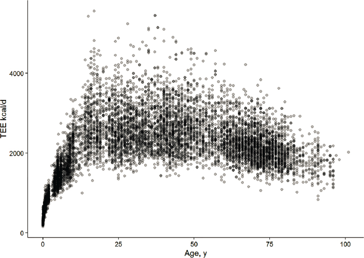
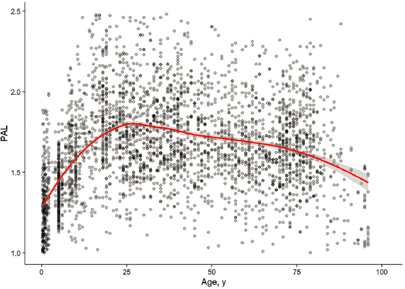
The non-linear relationship of TEE over age is shown in Figures 1 and 2 below (as well as in Appendix P §4).
___________________
19 NPNL is non-pregnant non-lactating but were women included in the studies of pregnant or lactating.
8.2 PAL Percentiles
PAL percentiles calculated from the imputed data were used to inform the quartiles by age group to use in classifying PAL levels. Bold numbers in Table 7 below were used to define the new age-dependent PAL categories as described above (Appendix Q §2.1).
TABLE 7 PAL Percentiles from Imputed Data by Age Categories (Appendix Q §2.1.1)
| Percentile | 0–2.99 y n = 750 | 3–8.99 y n = 926 | 9–18.99 y n = 704 | 19–70.99 y n = 4299 | 71+ y n = 1281 | Lactating n = 203 | Pregnant n = 431 | |||
|---|---|---|---|---|---|---|---|---|---|---|
| 10% | 1.00 | 1.20 | 1.34 | 1.39 | 1.31 | 1.34 | 1.30 | |||
| 25% | 1.11 | 1.31 | 1.50 | 1.53 | 1.46 | 1.50 | 1.46 | |||
| 50% | 1.27 | 1.44 | 1.66 | 1.68 | 1.62 | 1.69 | 1.60 | |||
| 75% | 1.44 | 1.59 | 1.85 | 1.85 | 1.79 | 1.83 | 1.77 | |||
| 90% | 1.61 | 1.75 | 2.04 | 2.03 | 1.95 | 2.05 | 1.97 | |||
| Percentile | 0–6 mo n = 443 | 7–11 mo n = 112 | 1–3 y n = 243 | 4–8 y n = 878 | 9–13 y n = 304 | 14–18 y n = 403 | 19–30 y n = 1,417 | 31–50 y n = 1,994 | 51–70 y n = 1,519 | ≥ 71 y n = 1,281 |
| 10% | 1.00 | 1.08 | 1.06 | 1.20 | 1.29 | 1.40 | 1.35 | 1.39 | 1.39 | 1.31 |
| 25% | 1.07 | 1.19 | 1.17 | 1.32 | 1.44 | 1.56 | 1.50 | 1.53 | 1.52 | 1.46 |
| 50% | 1.23 | 1.31 | 1.33 | 1.44 | 1.59 | 1.73 | 1.67 | 1.69 | 1.67 | 1.62 |
| 75% | 1.40 | 1.47 | 1.49 | 1.60 | 1.77 | 1.92 | 1.85 | 1.86 | 1.82 | 1.79 |
| 90% | 1.58 | 1.65 | 1.64 | 1.76 | 1.92 | 2.11 | 2.05 | 2.03 | 1.99 | 1.95 |
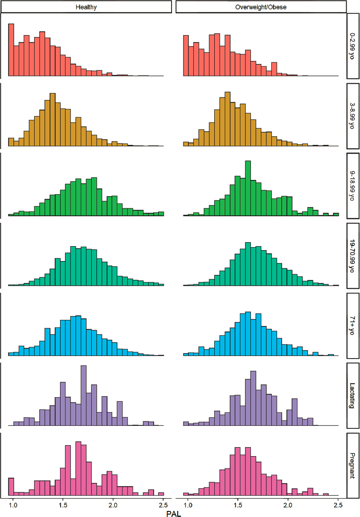
The distribution of PAL within age group is shown in Figure 3 (and Appendix Q §2.2).
8.3 TEE Equations
Final TEE models with coefficients for age, height, and weight by PAL category (Sedentary, Low Active, Active, Very Active) and age/sex strata are as follows (from Appendix Q §11):
Women, 19 years and above
- Sedentary: 584.90 – 7.01 Age (y) + 5.72 Height (cm) + 11.71 Weight (kg)
- Low Active: 575.77 – 7.01 Age (y) + 6.60 Height (cm) + 12.14 Weight (kg)
- Active: 710.25 – 7.01 Age (y) + 6.54 Height (cm) + 12.34 Weight (kg)
- Very Active: 511.83 – 7.01 Age (y) + 9.07 Height (cm) + 12.56 Weight (kg)
Men, 19 years and above
- Sedentary: 753.07 – 10.83 Age (y) + 6.50 Height (cm) + 14.10 Weight (kg)
- Low Active: 581.47 – 10.83 Age (y) + 8.30 Height (cm) + 14.94 Weight (kg)
- Active: 1004.82 – 10.83 Age (y) + 6.52 Height (cm) + 15.91 Weight (kg)
- Very Active: –517.88 – 10.83 Age (y) + 15.61 Height (cm) + 19.11 Weight (kg)
Girls, 3 to 18 years old
- Sedentary: 55.59 – 22.25 Age (y) + 8.43 Height (cm) + 17.07 Weight (kg)
- Low Active: –297.54 – 22.25 Age (y) + 12.77 Height (cm) + 14.73 Weight (kg)
- Active: –189.55 – 22.25 Age (y) + 11.74 Height (cm) + 18.34 Weight (kg)
- Very Active: –709.59 – 22.25 Age (y) + 18.22 Height (cm) + 14.25 Weight (kg)
Boys, 3 to 18 years old
- Sedentary: –447.51 + 3.68 Age (y) + 13.01 Height (cm) + 13.15 Weight (kg)
- Low Active: 19.12 + 3.68 Age (y) + 8.62 Height (cm) + 20.28 Weight (kg)
- Active: –388.19 + 3.68 Age (y) + 12.66 Height (cm) + 20.46 Weight (kg)
- Very Active: –671.75 + 3.68 Age (y) + 15.38 Height (cm) + 23.25 Weight (kg)
Girls, 0 to 2 years old
- –69.15 + 80.00 Age (y) + 2.65 Height (cm) + 54.15 Weight (kg)
Boys, 0–2 years old
- –716.45 – 1.00 Age (y) + 17.82 Height (cm) + 15.06 Weight (kg)
Pregnant women
- Sedentary: 1131.20 – 2.04 Age (y) + 0.34 Height (cm) + 12.15 Weight (kg) + 9.16 Weeks pregnant
- Low Active: 693.35 – 2.04 Age (y) + 5.73 Height (cm) + 10.20 Weight (kg) + 9.16 Weeks pregnant
- Active: –223.84 – 2.04 Age (y) + 13.23 Height (cm) + 8.15 Weight (kg) + 9.16 Weeks pregnant
- Very Active: –779.72 – 2.04 Age (y) + 18.45 Height (cm) + 8.73 Weight (kg) + 9.16 Weeks pregnant
Model coefficients are shown here for the primary models, including all BMI levels. Coefficients for sensitivity analyses removing high and low BMI or separated for “healthy” or “overweight/obese” are included for each strata in Appendix Q §3 (Women 19+) through §9 (Pregnant).
8.4 Model Performance
Model performance and validation is outlined in the “Performance-Report.” A summary of model fit measures for the primary models including all BMI levels are listed here in Table 8 (Appendix R §1.8).
TABLE 8 Model Fit for Each Age/Sex Stratum (Appendix R §1.8)
| Strata | n | R2 | R2 adj | R2 shr | r | MSE | RMSE | MAPE (%) | MAE |
|---|---|---|---|---|---|---|---|---|---|
| Adult Women 19+ | 1342 | 0.71 | 0.70 | 0.70 | 0.84 | 60393.43 | 245.75 | 8.67 | 190.89 |
| Adult Men 19+ | 1016 | 0.73 | 0.73 | 0.73 | 0.86 | 114615.05 | 338.55 | 9.35 | 265.54 |
| Girls 3–18 | 477 | 0.84 | 0.84 | 0.83 | 0.92 | 56049.24 | 236.75 | 8.19 | 165.44 |
| Boys 3–18 | 250 | 0.92 | 0.92 | 0.92 | 0.97 | 66831.33 | 258.52 | 7.11 | 163.25 |
| Girls 0–2 | 432 | 0.83 | 0.83 | 0.83 | 0.91 | 9059.24 | 95.18 | 12.80 | 73.51 |
| Boys 0–2 | 317 | 0.83 | 0.83 | 0.83 | 0.91 | 10732.61 | 103.60 | 13.56 | 79.47 |
| Pregnancy | 413 | 0.63 | 0.62 | 0.61 | 0.80 | 79769.92 | 282.44 | 8.80 | 222.10 |
R2 adj = adjusted R2, R2 shr = shrunken R2, as described in methods above, along with MSE, MAPE, and MAE.
Table 9 shows the mean and standard deviation of the difference in observed TEE – predicted TEE (i.e., the error) from the primary models in each stratum (Appendix R §1.10). The mean of the error is useful as a measure of bias, indicating a general tendency for whether the true val-
ues tend to be above or below the predicted values. Bland-Altman plots20 are displayed in Appendix R §1.10 to visually display the differences in observed – predicted values
TABLE 9 Mean (Bias) and Standard Deviation of the Difference in Observed TEE – Predicted TEE, by Stratum (Appendix R §1.10)
| Strata | n | Mean | Std Dev. |
|---|---|---|---|
| Adult Women 19+ | 1342 | 0.611 | 245.842 |
| Adult Men 19+ | 1016 | 29.387 | 337.437 |
| Girls 3–18 | 477 | 11.452 | 236.718 |
| Boys 3–18 | 250 | 43.162 | 255.400 |
| Girls 0–2 | 432 | 0.510 | 95.289 |
| Boys 0–2 | 317 | 0.059 | 103.762 |
| Pregnancy | 413 | 39.593 | 279.986 |
Prediction Error was calculated to show the precision of estimates if a new person’s TEE was predicted based on their age, height, weight, and PAL. We first calculated the predicted TEE and Standard Error (SE) based on a person at an average level of age, height and weight, with an “Active” PAL level within each strata (Table 10A, Appendix Q §10.1) and then also for someone above average (2 standard deviations above the mean) (Table 10B, Appendix Q §10.2).
TABLE 10A Prediction Error for Estimating a New Person’s TEE at Average Levels of Age, Height, and Weight, with “Active” PAL level (Appendix Q §10.1)
| Strata | Age | Height | Weight | Weeks preg | Predicted TEE | SE of the predicted value |
|---|---|---|---|---|---|---|
| Adult Women 19+ | 53.87 | 162.34 | 71.87 | — | 2,280.94 | 240.93 |
| Adult Men 19+ | 50.25 | 175.92 | 83.10 | — | 2,930.26 | 342.37 |
| Girls 3–18 | 9.58 | 135.02 | 37.63 | — | 1,872.65 | 221.06 |
| Boys 3–18 | 8.65 | 134.03 | 37.06 | — | 2,098.77 | 257.61 |
___________________
20 P. S. Myles, J. Cui, I. 2007. Using the Bland–Altman method to measure agreement with repeated measures, BJA: Brit J Anaesthesia 99(3):309–311. https://doi.org/10.1093/bja/aem214.
| Strata | Age | Height | Weight | Weeks preg | Predicted TEE | SE of the predicted value |
|---|---|---|---|---|---|---|
| Girls 0–2 | 0.72 | 68.31 | 7.81 | — | 592.58 | 95.87 |
| Boys 0–2 | 0.69 | 68.46 | 8.03 | — | 623.81 | 104.42 |
| Pregnant | 29.40 | 164.13 | 74.89 | 19.86 | 2,679.76 | 302.35 |
TABLE 10B Prediction Error for Estimating a New Person’s TEE at 2 SD above Average Levels of Age, Height, and Weight, with “Active” PAL level (Appendix Q §10.2)
| Strata | Age | Height | Weight | Weeks preg | Predicted TEE | SE of the predicted value |
|---|---|---|---|---|---|---|
| Adult Women 19+ | 53.87 | 169.43 | 87.99 | — | 2,526.23 | 241.28 |
| Adult Men 19+ | 50.25 | 183.46 | 99.55 | — | 3,241.22 | 343.32 |
| Girls 3–18 | 9.58 | 157.71 | 57.12 | — | 2,496.52 | 223.35 |
| Boys 3–18 | 8.65 | 161.26 | 58.34 | — | 2,878.92 | 262.99 |
| Girls 0–2 | 0.72 | 78.81 | 10.36 | — | 758.52 | 96.96 |
| Boys 0–2 | 0.69 | 79.06 | 10.76 | — | 853.83 | 105.88 |
| Pregnant | 29.40 | 170.72 | 95.07 | 19.86 | 2,931.34 | 306.19 |
8.5 External Validation
Model fit statistics were used to evaluate the out-of-sample data as described above. Tables 11A and 11B show the model fit from the predicted values after applying the TEE models to the study-level data extracted from the literature (Appendix R §4.2). The analyses were performed first for the studies with PAL available, with the second imputing PAL using Schofield equations based on the study averages for age, height, and weight.
TABLE 11A Model Fit from External Validation with Complete Data for PAL (Appendix R §4.2.1)
| Strata | n | R2 | r | MSE | RMSE | MAPE (%) |
|---|---|---|---|---|---|---|
| Boy | 8 | 0.90 | 0.96 | 95,651.47 | 309.28 | 7.90 |
| Girl | 7 | 0.82 | 0.97 | 56,812.37 | 238.35 | 10.38 |
| Man | 14 | 0.85 | 0.93 | 45,699.40 | 213.77 | 6.00 |
| Woman | 25 | 0.85 | 0.94 | 44,940.87 | 211.99 | 6.83 |
TABLE 11B Model Fit from External Validation with PAL Imputed for Schofield Equations (Appendix R §4.2.2)
| Strata | n | R2 | r | MSE | RMSE | MAPE (%) |
|---|---|---|---|---|---|---|
| Boy | 21 | 0.92 | 0.96 | 61,755.86 | 248.51 | 7.72 |
| Girl | 20 | 0.87 | 0.97 | 35,342.89 | 188.00 | 8.01 |
| Man | 32 | 0.82 | 0.92 | 49,684.74 | 222.90 | 5.57 |
| Woman | 71 | 0.82 | 0.93 | 28,833.66 | 169.80 | 5.46 |
9. APPENDICES21
| Appendix | Description |
| Appendix N | DLW Data Codebook |
| Appendix O | Data Preparation and Preliminary Descriptive Statistics |
| Appendix P | Clean Analysis |
| Appendix Q | Multiple Imputation GLM Results |
| Appendix R | Performance Report |
| Appendix S | List of IAEA Studies with Inclusion/Exclusion |
___________________
21 All appendixes to this IU report are provided in Supplemental Appendixes N through W and are available at: https://nap.nationalacademies.org/catalog/26818.
| Appendix T | IOM Data Extracted from 2002/2005 Report |
| Appendix U | External Validation Data |
| Appendix V | SAS Code for Importing, Harmonizing, and Merging Data |
| Appendix W | SAS Code for Multiple Imputation and Models |
Addendum to Appendix G
Details of Redefining of the TEE Model
As described in Chapter 5, a general model of TEE used age, height, weight, and PAL category as predictors and also included interactions of the PAL category with height and weight. The model performed to predict TEE used the following format:
where PALCATi represents 3 indicator variables for PAL category (Active, Low Active, Inactive) that are coded as 0 or 1; ‘A’, ‘B0’, ‘C0’, and ‘Di’ are the model coefficients for the main effects of age, height, weight and the 3 PAL categories, respectively; and ‘IBDi’ and ‘IBCi’ are the model coefficients for the interaction of the 3 PAL categories with height and weight, respectively. (The full model output including all the coefficients for interaction terms of height and weight by PAL category are provided in supplemental Appendix Q1). Moving the main effect of PAL category, and regrouping the terms by height and weight yields:
___________________
1 Supplemental appendixes are available at: https://nap.nationalacademies.org/catalog/26818.
In this model, the intercept represents the mean TEE level when Age, Weight, and Height are all 0. Obviously, this does not occur, and therefore it is not meaningful by itself, and, could even be negative. The coefficients for Age, Height, and Weight may be thought of as slopes—i.e., positive slopes represent increasing energy expenditure and negative slopes decreasing energy expenditure for a change in the corresponding variable holding the other values constant (e.g., for adult females, there is on average a decrease of 10.83 kcal/d for each 1-year increase in age, for women of the same weight, height, and physical activity level). The interaction terms allow the height and weight effects to differ for each PAL category, and the interaction coefficient (IBDi for height, ICDi for weight) represents the deviation from the referent group (Very Active).
Recognizing that PALCATi represents 3 indicator (0 or 1) variables (i=Active, Low Active, Inactive) and that Very Active is the reference category (all 3 are 0), we can write the predicted value for each category by substituting the 0 or 1 for PALCATi. For example, for the Active group:
which, after multiplying by the indicator values of 0 or 1, simplifies to:
where InterceptActive = Intercept0 + DActive.
This equation can be written simply as:
where ‘A’ is the same as above, ‘Intercept’ represents the sum of the intercept in the full model (Intercept0) and the ‘Di’ coefficient for the indicator for the PAL category, ‘B’ is the sum of the ‘B0’ coefficient from the full model and the ‘IBDi’ coefficient from the full model for the corresponding
PAL category, and ‘C’ is the sum of the ‘C0’ coefficient from the full model and the ‘ICDi’ coefficient from the full model for the corresponding PAL category. All PAL levels could be predicted in the same manner. For the special case of the referent group (Very Active), all indicator variables are 0, so the prediction is simply:
which also simplifies to the equation directly above.
DIFFERENCE IN EQUATIONS COMPARED TO THE 2005 EER:
For the 2005 EER, the following prediction of TEE was used:
where ‘A’, ‘B’, and ‘C’ are the coefficients for age, height, and weight respectively, and ‘PA’ is a coefficient for each PAL category that is multiplied by both height and weight. By substitution of the four coefficients for PA, this prediction could also be written separately for each PAL category, as above. Also, similar to the TEE prediction equation above, the coefficient for Age remains constant for each PAL category. However, in contrast to the TEE prediction equation above, the intercept also remains constant, and, although the coefficients for Height and Weight vary by PAL category, they are mutltiplied by the same PA coefficient, whereas in the equation above, the parameters represent a deviation from the overall slope, which is not restricted to be the same for height and weight. A comparison of the EER values from 2005 and 2023 is presented in Chapter 7.


