Possible Health Effects of Exposure to Residential Electric and Magnetic Fields (1997)

This chapter provides an overview of various aspects of exposure to electric and magnetic fields that are considered relevant to the understanding of biologic interactions evaluated in other chapters. No attempt was made to be comprehensive; rather the goal was to provide a brief introduction to the tools necessary for exposure analysis. References to published comprehensive reviews and reports are given.

The following general conclusions are derived from the review of the literature presented in this chapter:

• Ambient levels of 60-Hz (or 50-Hz in Europe and elsewhere) magnetic fields in residences and most workplaces are typically in the range of 0.01-0.3 µT (0.1-3 mG). Higher levels are encountered directly under high-voltage transmission lines and in some occupational settings. Some appliances produce magnetic fields of up to 100 µT (1 G) or more in their vicinity.

• Exposure levels of electric fields and other characteristics of magnetic fields (harmonics,¹ transients,² spatial, and temporal changes) have received relatively little attention in the studies of possible biologic and health effects.

• Indirect estimates of human exposure to magnetic fields have been commonly used in epidemiology (e.g., calculations, ''wire codes" (see Glossary and Appendix B for definitions of wire codes), distance, and contemporary measurements).

• Wire codes, the most commonly used estimates of possible exposure to electric and magnetic fields, are not strong predictors of magnetic-field strengths in homes. Within a given geographic region, however, wire codes to tend to distinguish relatively well between the higher and lower field strengths in homes.

• Exposure of humans and animals to 60-Hz electric and magnetic fields induces currents internally. The density of these currents is nonuniform throughout the body. Also, the spatial patterns of the currents induced by the magnetic fields are different from those induced by the electric fields.

• The endogenous current densities on the surface of the body (higher densities occur internally) associated with electric activity of nerve cells (as measured by electroencephalograph) are of the order of 1 milliampere per square meter (mA/m²) and are chiefly of even lower frequency than 60 Hz, peaking at 5-15 Hz. Human exposure to a 60-Hz field of 100 µT (1 G) is needed to produce an equivalent current density in the body. The induced current densities caused by typical residential fields (about 1 mG) are therefore about 1 µA/m², or 1,000 times less than endogenous current densities.

• Microscopic heterogeneity has not been accounted for in evaluations (experimental or theoretic) of local current densities within tissues and in and around cells and cell assemblies.

• Several features are required for laboratory field-exposure systems to help eliminate potential experimental artifacts. Relatively few experimental studies have reported using systems that satisfy all these requirements. One requirement, obtaining and analyzing the data blind to the status of the exposure conditions, is extremely important. A large fraction of the published reports either do not provide sufficient information or do not satisfy many of the requirements for appropriate exposure-system design and operation.

Electric and magnetic fields are produced by electric charges and their motion. A static electric field is produced by electric charges whose magnitude and position do not change in time. A static magnetic field can be produced either by a permanent magnet or by a steady flow of electric current (moving electric charges). The magnetic field produced by the latter means is frequently called a direct-current (dc) magnetic field. Alternating-current (ac) magnetic fields are produced by electric currents alternating in time. Electric and magnetic fields are vector quantities and thus are characterized by their magnitude and direction at every point in space and time. The behavior of electric and magnetic fields and their interrelationship are comprehensively described by Maxwell's equations

(see Peck 1953; Kraus 1992; Iskander 1993; or other general texts on electromagnetic theory). One of the primary features of electric-and magnetic-field behavior is that a time-varying electric field produces a magnetic field and vice versa; therefore, reference is often made to the electromagnetic field. This field behavior, and simultaneous existence of both field components, occurs at all frequencies. However, for slowly varying fields (low frequencies), either the electric field or the magnetic field can predominate (i.e., much stronger in terms of the energy associated with it). Frequencies associated with power lines and their common harmonics are low enough for electric fields and magnetic fields generated by them to be considered separately (i.e., uncoupled). The physical reason for this simplification is that the electric field induced by the magnetic field (or vice versa) is proportional to the time rate of change. Quantitatively, one can consider the fields separately, if the magnetic field produced by the original magnetic field via the induction of the electric field is only a very small fraction of the original field. Furthermore, the common sources of the fields of low frequencies are generally separated from the exposed person, experimental animal, or cells by distances much smaller than the wavelength of the exposure field. (The electric and magnetic fields are not related through the plane wave intrinsic impedance, because no such waves are formed.) At frequencies above a few kilohertz, more careful consideration needs to be given to the coupling of the electric and magnetic fields.

An electric field is described by its strength (designated ) (a bar over the field symbol indicates a vector) and its displacement vector (), also called the electric flux density. The two vectors are interrelated by the electric properties of the medium:

where ∈ is the medium permittivity; for free space î = î₀. For biologic materials, the permittivity is a complex number consisting of a dielectric constant and a loss factor (related to the conductivity). The electric field is measured in volts per meter (V/m), and the electric flux density in coulombs per square meter (C/m²).³

A magnetic field is described by its strength () and the magnetic flux density (). The two vectors are related by magnetic properties of the medium:

where µ is the medium permeability; for free space µ = µ₀. For most biologic materials (except magnetite found in small quantities in some tissues), µ = µ₀. The most commonly used magnetic-field descriptor is its flux density presented either in units of tesla (T), an internationally approved (SI) unit, or an older and

more common unit of gauss (G), (1 G = 10^-4 T; also 1 T = 1 Wb/m², where Wb = weber). The magnetic-field strength has units of amperes per meter (A/m).

One of the characteristics of an ac electric or magnetic field is its waveform (i.e., the change in amplitude and phase with time). Sinusoidal (harmonic) fields of 50 or 60 Hz are the most commonly encountered ac fields in the environment, and they are often used in biologic experiments. They can also contain small distortions resulting in harmonics (multiples of the fundamental frequency, e.g., 120 Hz, 180 Hz, etc., for the 60-Hz fundamental frequency). Another common waveform used in the laboratory is a "rectangular" pulse or a time series of pulses either bipolar or unipolar. A whole range of frequencies are associated with a pulse or a series of pulses. The exact frequency spectrum depends on the pulse characteristics, such as its duration, repetition rate (for multiple pulses), the rise time (of the leading edge), and the fall time (of the trailing edge). In technical terms, these frequencies are determined by Fourier analysis. A brief discussion of the spectra of simple waveforms is given in a report by ORAU (1992). Waveforms associated with some phenomena, such as lightning and on and off switching of electric devices, are frequently referred to as transients and are very complex and unique for a given event. Their frequency spectra are broad and extend into the megahertz range.

A parameter characterizing the field and related to its frequency (for harmonic fields) is the wavelength. The wavelength in free space is related to frequency in free space as

where c is the velocity of light (c = 3 × 10⁸ m/sec). In media, such as biologic tissues, the wavelength is shorter than that in free space and equal to

where ∈ is the permittivity of the tissue in question; it should be noted that various tissues have different permittivities.

The range of frequencies in which the power-line fundamental frequencies of 50 or 60 Hz fall is referred to as extremely low frequencies (ELF). ELF are generally considered to extend from 3 Hz to 3 kHz.

The electric field at power-line frequencies produced by specific voltages on high-voltage transmission lines can be accurately evaluated by analytic or numeric methods. Similarly, for distribution lines and any other known configuration of wires and other shape conductors, it is possible to evaluate the strength and direction of the electric field in any point of the surrounding space. Simple cases, such as a plate, a single straight wire (in free space), a wire above ground, two wires (infinitely long), three phase wires, and similar configurations, can be

solved analytically. Several examples are given in the ORAU (1992) report. It is important, however, to realize that the electric field is significantly perturbed by any conducting or dielectric object that is placed in it. Thin objects placed perpendicularly to the direction of the field introduce only a minimal field perturbation. That feature of electric fields has a significant bearing on correct measurements of the fields. People and animals greatly affect the field (Kaune and Gillis 1981). Therefore, the measured field in the presence of a person is significantly different from the exposure field without the person present.

Similarly to the electric field, the magnetic field can be accurately evaluated (analytically or numerically) for various configurations of current-carrying conductors. Examples of simple calculations are given in the ORAU (1992) report. For any arbitrary but known configuration of conductors, the magnetic field can be computed numerically. In cases of motors and other devices of complex geometry, particularly those containing magnetic materials, theoretic evaluation of the exposure field is impractical. Unlike the electric field, the ELF magnetic field is not affected by the presence of humans and animals. Therefore, the measured field represents the actual exposure field.

Electric and magnetic fields at 60 (or 50) Hz can be calculated or measured in practically any environment. Even their more complex characteristics (e.g., harmonics and temporal and spatial changes) can be determined. Similarly, transients can be measured, albeit only with sophisticated instrumentation. Determination of human exposure and, in particular, determination of human exposure as it relates to epidemiologic studies is much more difficult. An average adult or child encounters a variety of environments of electric and magnetic fields in a day, not to mention in a month or a year.

The original interest in possible health effects of power-line fields was precipitated by an epidemiologic report (Wertheimer and Leeper 1979), which suggested that the strength of 60-Hz magnetic fields, as classified or estimated by a wire code, correlates with increased rates of childhood cancers, including leukemia. In subsequent studies, wire codes, or other presumed indicators of the average root-mean-square (rms) strength of the 60-Hz magnetic field, have been used.

Various characteristics of electric and magnetic fields, other than their rms magnitude at 60 Hz, might be responsible for their interaction with biologic systems (e.g., harmonics, transients, and temporal and spatial changes). Knowledge of which characteristic (if any) of the exposure fields is important in the interaction would permit reliable exposure assessment in epidemiologic studies. Lack of knowledge of the relevant field characteristic makes comprehensive

human exposure assessment nearly intractable. Nevertheless, a majority of studies have been conducted with the tacit assumption that the 60-Hz magnetic field (rms averaged and cumulative over time) is directly related to the exposure of interest.

Exposure can be assessed by direct measurements or by indirect modeling and estimation of the electric and magnetic fields present in the spaces occupied by humans or experimental animals. In most cases, such evaluations have been made at 60 (or 50) Hz only.

Without any clear guidance about what aspect of a field is biologically relevant, most commonly available field-measurement devices today have been designed to determine the average rms field strength (magnetic flux density or electric-field strength) over a specific time. The minimum averaging time is usually about 1 sec, and some instruments can average for hours. More elaborate equipment has the capability to measure the detailed time variation or frequency spectrum of a field, but analyzing or choosing a simple metric from the enormous amount of information collected is difficult.

As a compromise, some of the more popular field-measurement devices today are able to record many samples of the magnetic field over a long period; for example, they can be set to record a sample every 10 sec for 24 hr. The resulting amount of data is manageable and permits the calculation of a limited range of summary metrics (such as average rms field, peak field, median field, difference between successive measurements, and time above a specific threshold).

Most of the monitoring devices for electric and magnetic fields use filtering to limit the range of frequencies measured. Such a device can measure a narrow band of frequencies from 50 to 60 Hz or cover a broad band of frequencies from 20 to 2,000 Hz. Regardless of the frequency range measured, the instruments report a single number reflecting the sum of all fields in that frequency range.

The most common method used to determine the electric field is to measure the voltage between two conductors. In one popular instrument, the two conductors are the upper and lower halves of the device case. Because the presence of the instrument user can alter the electric field, the sensing probe of the measurement device must be held away from the body by means of a long nonconducting rod. To make a reading, the user rotates the probe until its axis is parallel to the direction of the electric field (the maximum reading).

The most common method used to determine the magnetic field is to measure the voltage induced in a coil of wire by the alternating field. To make a reading, the coil must be rotated until its axis is parallel to the direction of the magnetic field. Some devices use a coil that is separate from the instrument electronics package; others incorporate the coil in the instrument case so that the entire

device must be rotated. More expensive devices for the measurement of magnetic fields use three orthogonal coils in the instrument case. Instead of having to rotate a single coil, the devices sense the three mutually perpendicular components of the field by these coils and calculate the vector sum of the fields. Procedures for measuring electric and magnetic fields in the environment are described in detail by ANSI/IEEE (1987).

For well-defined sources, magnetic flux densities can be calculated accurately, and measurements support the accuracy of such calculations. Electric fields can also be calculated, but because the fields are perturbed by conducting objects, calculations are often of limited value unless the perturbations by such objects can be modeled. Electric-and magnetic-field calculations, when properly performed, are more accurate than measurements; in fact, field-measuring devices are frequently calibrated against the calculated field of a simple geometric arrangement of conductors.

For most environments (in the home or workplace), conductor geometries are complex or unknown, so measurements must be used. For distribution lines, even though the geometry is relatively simple, the currents are not the same in each wire (not balanced) and are generally not known accurately enough to rely on calculations. For transmission lines, however, the amount of power transmitted is generally recorded, and the line currents are usually balanced sufficiently to be estimated accurately; therefore, the field can be calculated accurately, assuming no other sources or shielding materials are near.

Exposure to electric fields in the home and workplace environments can be attributed primarily to electric equipment used in those environments. Because of the ease with which very-low-frequency 60-Hz electric fields are shielded or perturbed, electric fields in the home and workplace have not been characterized satisfactorily. Attempts have been made to measure personal exposure to electric fields (e.g., by the Electrical Power Research Institute (EPRI 1990)), but the measurements are heavily dependent on where the exposure meter is worn, the orientation of the exposure meter, and the presence of any conductors near the exposure meter. With that caveat, EPRI found that the mean personal exposure to 60-Hz electric fields in the home or office typically ranges from 5 to 10 V/m.

Power-line electric fields have been well characterized; depending on line voltage, ground-level electric fields under a line might be as high as 10 kV/m, which is sufficient to cause fluorescent tubes to glow and to induce noticeable

shock currents in a person who touches a vehicle parked under a high-voltage line. Mean personal exposure to electric fields for substation, distribution-line, and transmission-line workers ranges from 50 to 5,000 V/m (EPRI 1990).

The three most common sources of residential 60-Hz magnetic fields are electric appliances, the grounding system of the residences (most often, water pipes), and nearby power lines (most commonly, low-voltage distribution lines). Normally, unless there are wiring anomalies, internal residential wiring is not a significant source of personnel exposure. Although high-voltage transmission lines produce relatively high magnetic fields directly under them, they contribute relatively little to the residential and environmental levels at distances greater than 100 m, as illustrated in Table 2-1.

The background magnetic fields in the center of the rooms (away from most appliances) of the home are most likely caused by power lines, grounding systems, or some combination of the two. In an EPRI (1993a) study in which extensive magnetic-field measurements were taken in the center of the rooms of 992 homes, only 5% of the homes had average magnetic fields exceeding 0.29 µT (2.9 mG).

The distribution of fields observed for selected rooms in the homes and the all-room averages are shown in Table 2-2. Assuming people's activity patterns are uniformly distributed within the residence living space, the all-room average field shown in Table 2-2 should provide a slightly better characterization of exposure than the all-room median field (not shown in the table) (EPRI 1993a). Household energy consumption and the presence of electric heating did not explain variations in the measured magnetic fields between homes (EPRI 1993a).

In the EPRI study, the power-line fields were found to be the dominant source of average and median fields. For most low-voltage power lines, the load current on the three wires is not always balanced. To analyze the effect of the imbalance, the load current can be mathematically divided into the balanced and unbalanced parts; the balanced part of the current produces a field that decreases approximately as the inverse square of the distance from the power line; the unbalanced part (the zero-sequence current) causes a field that decreases with the inverse of the distance. Therefore, at greater distances, the field associated with the zero-sequence current dominates. When the median field in a house is greater than 0.16 µT (1.6 mG), the home in question is usually near a power line and the main field source is usually the balanced part of the power-line load current.

The strongest magnetic fields in homes are generally caused by appliances. However, the fields usually decrease rapidly with distance. When the main source of a magnetic field in an appliance is a coil of wire, the field decreases approximately as the inverse cube of the distance. Some of the magnetic-field values measured near household and other appliances are shown in Tables 2-3 and 2-4. The values show the range of all the measurements made (e.g., 95% of the color television sets measured emitted magnetic fields less than 0.33 µT at a distance of 56 cm). The values are based on measurements of the rms fields averaged over time from about 1 sec or more for the spot measurements to 24 hr for long-term and personal exposure measurements. Different appliances of the same type can produce different magnetic fields because of differences in their design. Important differences are the amount of current they use, the size and shape of conducting parts, the number of turns of wire in coils, and whether shielding or field-canceling technology was used.

In addition to the appliances listed in Tables 2-3 and 2-4, magnetic fields from electric blankets might contribute a large part to the magnetic-field exposures in the home. When measured about 5 cm from the surface of the blanket, approximately the distance of internal organs, the magnetic fields average about 2.2 µT (22 mG) for conventional electric blankets and about 0.1 µT (1 mG) for positive-temperature-coefficient blankets.

Because the subject moves around the house during personal-exposure measurements, personal exposures include contributions from electric appliances as well as from power lines and grounding systems. The contribution of appliances to total exposure can be seen in Table 2-5. The values shown include personal exposures and long-term stationary measurements made using the same instrumentation. The personal-exposure measurements are consistently higher than the measurements made at fixed positions in the rooms. The fixed-position measurements were made in a frequently used room, other than the bedroom, and away from any identifiable local magnetic-field source (EPRI 1993b).

Several studies have examined the personal exposures of children (e.g., Kaune et. al. 1994). The personal exposures were approximately log-normally distributed with both residential and nonresidential geometric means of 0.1 µT (1 mG). The correlation between log-transformed residential and total personal-exposure levels was 0.97. This close correlation might be due to the fact that children spend most (two-thirds to three-fourths) of their time at home.

In the EPRI residential study (EPRI 1993b), short-duration measurements were made in the center of the rooms and outdoors around the perimeter of the

house. The two sets of measurements were similar; both included contributions from the grounding system and nearby power lines. At greater distances from a home, the magnetic field is controlled primarily by components of the power-delivery system, including distribution-system primary and secondary wires and transmission lines.

Transformers and substations are usually not important sources of magnetic fields in a community (beyond the substation boundary). However, because substations represent a point of convergence for power lines, residences near substations have a greater chance of being near power lines and, therefore, have a greater chance of exposure to higher magnetic-field levels from the power lines. Also, some power lines might be closer to the ground near the substation, thus causing the ground-level fields to be greater. In addition, there might be higher ground-level return currents in the earth near substations and therefore higher field levels in the area.

For homes near transmission rights-of-way, transmission lines can be important sources of magnetic fields. Typical values for the magnetic fields from transmission lines were illustrated in Table 2-1 (EPA 1992). At peak usage, the magnetic fields could be double the average figures shown in the table. Note that the fields fall off roughly as the inverse square of the distance from the line, and the magnetic field is greater for the higher-voltage lines. There are two reasons the magnetic field is greater for the higher-voltage lines: higher-voltage lines generally have thicker wires to carry more current (magnetic field is directly proportional to current); and higher-voltage lines have a greater separation between wires to avoid arcing. The magnetic fields produced by the three conductors of a three-phase transmission line tend to cancel one another. Greater wire spacings result in less cancellation; closer spacings result in more cancellation. If the three phases could occupy the same space, the fields would exactly cancel each other and a balanced (in current and phase angle) three-phase transmission line would produce zero magnetic field. That situation is approximated when the wires are insulated and placed together in an underground pipe.

The electric power lines commonly observed in neighborhoods are usually not transmission lines as described above, but are lower-voltage distribution lines. The magnetic fields near distribution lines are generally around 0.5 µT (5 mG), but in some densely populated areas, field levels as high as 5.0 µT (50 mG) have been measured.

There are two major types of underground power lines: direct burial (the individual wires are buried separately) and pipe-type cables (all the wires are placed in a single metal pipe). Direct-burial underground power lines can produce ground-level magnetic fields as large as equivalent capacity overhead lines (but over a more limited area). Although the underground wires might be closer

together than overhead wires (tending to decrease the field), they are buried at a depth of only about 5 ft and, therefore, are much closer to the surface of the ground than overhead lines (a fact that tends to increase the field). In underground pipe-type transmission lines, the close spacing of the wires in the pipe and the metal pipe itself decrease the magnetic field, so that the resulting ground-level field is typically less than 0.1 µT (1 mG).

The magnitude of the magnetic field for the office environment is similar to that for the home; however, differences might exist in the extent and pattern of exposure to electric devices. Typical magnetic fields from workplace equipment are illustrated in Table 2-6 (EPA 1992). Note that the fields for a particular type of device (e.g., copy machines) vary greatly from one machine to another because of the amount of current used and other design features. The data are missing for the lowest-field fluorescent light because its field was less than the background field. Compact fluorescent lights, which are being used extensively in the workplace as a more efficient replacement for incandescent lights, produce negligible magnetic fields at 2 ft because of their compact size and low current use.

In a study of occupational exposures (EPRI 1990), personal-exposure measurements were performed in the home and workplace. As Table 2-7 shows, the home and office are similar magnetic-field environments; however, office exposures are somewhat higher, possibly reflecting more frequent (or continuous) and proximal use of electric equipment. Measurements of the home environment provided in Table 2-7 are somewhat different from those in Table 2-5, because

the protocols of the two studies were different. Those differences make it difficult to make detailed comparisons between the studies.

In work environments involving high currents and large distances between the current-carrying conductors, such as substations and generating stations, magnetic fields are at high levels over large areas. In the occupational project by EPRI (1990), which included such utility-specific environments as substations, generating stations, and work areas involving transmission and distribution lines, the highest exposures were of workers in substations.

In another study that focused on the home exposure of adults (Kavet et al. 1992), the average exposure while away from home was relatively uniform at about 0.2 µT (2 mG) for the study population. That amount is consistent with the data for office workers shown in Table 2-7. However, the subjects spent a large fraction of their time at home, so their total exposures were similar to their at-home exposure.

Some transportation systems, including subways and intercity trains, operate on alternating current and generate ac electric and magnetic fields. As shown in Tables 2-8 and 2-9, magnetic fields in transportation environments are extremely variable. The temporal and spatial variations are great, and for some trains, large frequency variations occur as the speed of the trains changes.

Transients are present in all environments where switched equipment is used. A recent study of transients (EPRI 1994a) found that transients within the home can be random, originating from manual and automatic switching devices (such as those associated with lights and appliances), or repetitive, originating from electronic controllers (such as dimmer switches that produce transients twice per

power-frequency cycle). The rate of occurrence of transients is greater in industrial areas than in residential areas.

The frequencies associated with switching transients range from less than 60 Hz to about 500 MHz. Switching transients begin with high-frequency components radiated directly from the vicinity of the switch, followed by low-frequency components resulting from currents in residential and distribution wiring. Repetitive transients typically have a single dominant frequency component.

The measured amplitude of the magnetic flux density ranged from 0.001 µT (0.01 mG) to 10 µT (100 mG), depending on source, frequency, and position. Transients can propagate in residential wiring through secondary distribution lines to neighboring residences and along ground pathways (conductive plumbing pipes). Switching operations in primary distribution lines can generate transients within the residences (EPRI 1994a).

Personal exposure to transient fields is extremely complex because of their strong spatial dependence. Exposure to high-frequency fields is typically due to switching operations within the residence (e.g., light dimmer switches), but exposure to low-frequency fields can also be due to external sources in the neighborhood. The frequency and strength of the fields are such that transients can induce currents that are larger than thermal noise; thus, magnetic fields associated with

transients to which individuals might be frequently exposed could be considered in future research.

The primary hypothesis tested in most residential epidemiologic studies of electric-or magnetic-field effects is that the presence of power lines near the home is related to occurrence of disease. With few exceptions, the studies have focused on indirect estimates of the magnetic fields rather than electric fields. At low frequencies, such as 60 Hz, electric fields are substantially shielded by the shell of a house and by surrounding trees, so that residential exposure to electric fields is difficult to describe and nearly impossible to model with any accuracy. In the study by London et al. (1991), nearby power lines appeared to have no influence on indoor electric fields.

On the other hand, magnetic fields are largely unaffected by intervening structures and therefore might reflect more directly the operation of nearby power lines. Exposure assessments in the residential studies (e.g., wire codes and distance to power lines) have been viewed as estimates or indirect measurements of some aspect of magnetic-field exposure experienced by the subjects before their disease was diagnosed. Because of limitations in instrumentation or available data, the magnetic-field characteristic examined is usually a short-or long-term rms average field. Each of the exposure assessment methods has its strengths and weaknesses. The following sections briefly describe the major types of exposure assessment used.

This indirect measure was used in the first epidemiologic study of presumed exposure to magnetic fields and cancer risk (Wertheimer and Leeper 1979). This means of exposure quantification was subsequently used in later studies with several refinements and modifications. Categories of wire codes and how they relate to the high-voltage transmission and distribution lines are illustrated in Figure 2-1. Detailed information on wire codes can be found in Appendix B, and more details on their use in epidemiology are given in Chapter 5.

The use of the wire code illustrated in Figure 2-1 and its modifications has a qualitative physical rationale but also significant quantitative limitations. Its use in previous epidemiologic studies was based on the assumption that the wire code reflects the average exposure to 60-Hz magnetic fields. The rationale of this assumption is that larger power lines with thicker wires, which serve more residences and other consumers of electricity, carry more current and therefore provide a measure of exposure in the past and over a prolonged period. The

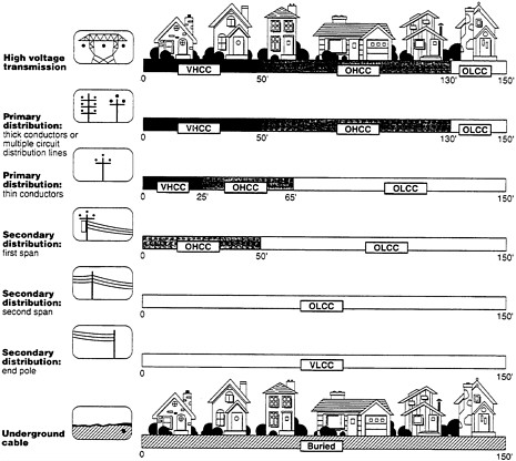
FIGURE 2-1 A simplified schematic of the basic features of the differences in the wire codes as defined to support epidemiologic studies. VHCC, OHCC, OLCC, and VLCC stand for very high, ordinary high, ordinary low, and very low current configurations. Figure provided courtesy of Robert S. Banks Associates, Inc. (originally prepared for EPRI and revised for this report).

merit of this rationale is that it considers (albeit in a qualitative manner) several of the factors used to calculate power-line magnetic fields; however, the reliability of the wire codes as a quantitative measure of exposure to 60-Hz magnetic fields is very limited. The following is a summary of some of the findings in a review of the characteristics of the wire codes as used in the epidemiologic studies:

• Although the rank ordering of fields in homes is predicted reasonably well by wire codes, the wire code accounts for only 15-20% of the variance in magnetic-field measurements.

• A large overlap exists between the estimated ranges of the magnetic fields for various categories (e.g., very high current configuration and ordinary high current configuration). There are large differences between the magnetic fields for different studies in different geographic locations for the same categories of the wire code. For instance,

•  In a comparison of Los Angeles, California, and Denver, Colorado, the differences between the cities within one category are greater than the differences between categories.

•  Total exposure to 60-Hz magnetic fields in single-family residences is affected by other factors (appliance fields and grounding system fields). The field from a power line adjacent to the residence is a dominant factor for high wire codes but not for low wire codes.

Figure 2-2 compares mean residential magnetic-field measurements by wire-code category for different studies (EPRI 1994b). The data were obtained by several different procedures. Indoor spot measurements were usually taken with hand-held meters for a brief time at a limited number of locations in the residence (usually at the center of rooms, where the fields from appliances and house wiring are not very significant). Stationary measurements were made with instruments left in the residence for an extended time (usually 24 hr or more); appliances and house wiring might contribute somewhat to the measured field. For personal-exposure measurements, the meter is always near the subject (either worn or placed on a bedside table); the contribution of appliances to the measured field is usually significant.

Six studies are represented in the graphs—three are epidemiologic studies, and three are exposure assessment studies. The author of the EPRI (1994b) report cautions that Figure 2-2 includes multiple data points of the same type of measurement from several studies to show some of the variation possible in arithmetic mean measurements under different conditions (e.g., spot measurements

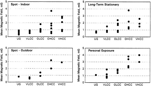
FIGURE 2-2 A comparison of mean residential magnetic-field measurements by wire-code category for six studies. Source: EPRI 1994b.

under low-and high-power usage conditions or personal exposures for children and adults in the same homes). Several studies using different methods are shown in Figure 2-2; therefore, some of the differences between measurements are undoubtedly due to the differences in study populations or study methods.

The possibility that wire codes better represent another characteristic of magnetic fields rather than their magnitude at 60 Hz is relatively unexplored so far. For instance, they might reflect the numbers and magnitude of transients. If laboratory studies had clearly indicated that 60-Hz magnetic fields were carcinogenic at such low levels as those considered in the epidemiologic studies, then there might be less concern about the limitations of the wire codes as measures of exposure.

Magnetic fields from power lines can be calculated accurately if the relevant variables are known. The most important variables for calculations are wire spacing and height, current in each wire, and distance to the residence. Utilities rarely have records of the current in each wire of a power line for past years (the prediagnosis period). More often, there is a record of power-line load from which current in each wire can be calculated, if it is assumed that the currents are balanced. Balanced current is usually a good assumption for high-voltage transmission lines but not for the more common low-voltage distribution lines. Because of these limitations, calculations are not often used. Historical records of power-line loads are sufficiently complete in Sweden, however, for Feychting and Ahlbom (1993) to use the calculated magnetic fields in their study.

Because the magnetic field decreases with distance from an operating power line, distance can be used as a crude predictor of the field. The utility usually has records showing whether a particular line was operating during the prediagnosis period. Because the actual field also varies with line load and the geometric configuration of the power line, the use of distance can result in significant misclassification, particularly if a study involves power lines of several different designs. Because of its simplicity, distance is frequently used as an exposure metric to assign subjects to two or more exposure groups.

Two types of measurements are used most often: spot measurements (the rms average magnetic field over a period of seconds or minutes), and a long-term rms average (a measurement extending 24-48 hr). The long-term average is frequently called the time-weighted average. A personal-exposure measurement

is a long-term average recorded by a measuring device worn by a subject. Other measurements, such as the peak field or field exceeded 10% of the time, are used occasionally.

Transmission-line measurements correlate well with calculated fields, but they only reflect line currents during the measurement period, which might or might not be typical for the power line. Measurements are the only practical way to determine the field from complex sources, such as distribution lines, appliances, and ground currents. A major criticism of contemporary magnetic-field measurements is that they might not reflect conditions accurately that prevailed years before—during the period the disease developed.

Occupational studies typically rely on job title as an indicator of a subject's magnetic-field exposure or on magnetic fields measured at representative work locations (either personal exposure or spot measurements) and combined with each subject's work history. Both methods are likely to result in misclassifications because of the large overlapping range of fields measured for a given job title (e.g., see the measurements reported by Theriault et al. 1994).

Electric Fields The most commonly used exposure apparatus consists of parallel plates between which an alternating voltage (50 or 60 Hz, or other frequencies) is applied to produce the electric field. Typically, one of the plates (bottom) is grounded. When proper dimensions of the plates are selected (large area in comparison to their separation), a uniform field can be produced within a reasonably large volume between the plates. Distribution of the electric-field strength within a volume of interest can be calculated. The field uniformity deteriorates close to the plate edges.

Electric fields of up to 100 kV/m have been used in experiments with animals. This field strength for a rodent corresponds to about 10 kV/m for a human, as described in the following section on in vitro studies.

The original reasonably uniform field in an animal-exposure system can be significantly perturbed by two factors. One factor, which is unavoidable but controllable, is due to the presence of test animals and their cages. A considerable amount of information is available on proper spacing of animals to ensure the same exposure field for all test animals (Kaune 1981a) and to limit the mutual

shielding of test animals (Kaune 1981b; Creim et al. 1984). Animal cages, drinking bottles, food, and bedding cause additional perturbation to the electric field (Kaune 1981a,b). Particularly, any metallic or other highly conductive objects or substances (e.g., animal excrement) must be eliminated or kept to a minimum. One of the most critical problems resulting in artifactual results of some studies is induction of currents in the nozzle of the drinking-water container. If the induced currents are sufficiently large, animals experience electric microshocks while drinking. Corrective measures have been developed to deal with this problem (Free et al. 1981; Kaune 1981b). Perturbation of the exposure field resulting from nearby metallic objects is easy to prevent.

Improper design, construction, and use of the electric-field-exposure facility can result in unreliable measurements. Therefore, unless sufficient information is given about the exposure system or an independent expert evaluates the system, the results of the studies might not be given full weight in this assessment. Table 2-10 summarizes essential specifications for any animal or in vitro experiment, whether exposure is to electric, magnetic, or combined electric and magnetic fields. The critical and desirable specifications that should be reported for each animal experiment in electric fields are listed in Table 2-11.

Magnetic Fields A magnetic field in an animal-exposure apparatus is produced by current flowing through an arrangement of coils. The apparatus can vary from a simple set of two Helmholtz coils (preferably square or rectangular because of the geometry of cages), to an arrangement of four coils (Merritt et al. 1983), to more complicated coil systems (Stuchly et al. 1991; Kirschvink 1992; Wilson et al. 1994; Caputa and Stuchly 1996). The main objectives in designing exposure apparatus for magnetic fields are (1) to ensure the maximal uniformity of the field within the largest volume encompassed by the coils, and (2) to minimize the stray fields outside the coils, so that sham-exposure apparatus can be placed in the same room. Square coils with four windings arranged according to the formulas of Merritt et al. (1983) are optimal in satisfying the field-uniformity requirement. Limiting the stray fields is a challenge, as shielding magnetic fields is much more complex than shielding electric fields. Nonmagnetic metal shields provide only a small reduction in the field strength. Only properly designed multilayer shielding enclosures made of high-permeability materials are effective. An alternative solution relies on partial field cancellation. Two systems of coils placed side by side or one above the other form a quadrupole system that results in a substantially faster decrease of the magnetic field as distance from the system is increased (Harvey 1987; Stuchly et al. 1991). An even greater decrease is obtained with a doubly compensating arrangement of coils. Four coils (each consisting of four windings) are arranged side by side and up and down; coils placed diagonally are in the same direction as the field, and the neighboring coils are in the opposite direction (Caputa and Stuchly 1996).

Common potential artifacts associated with magnetic-field-exposure systems are heating, vibrations, and audible or high-frequency (nonaudible for humans) noise. These factors can be minimized but not entirely eliminated with careful design and construction, which can be costly. The most economic and reliable way of addressing and solving these problems is through essentially identical design and construction of the field-and sham-exposure systems except for the current direction in bifilarly wound coils (Kirschvink 1992; Caputa and Stuchly 1996). This solution provides for the same heating in both systems. Vibration and noise are usually not exactly the same but are similar. To limit the vibration and noise, the coil windings should be restricted mechanically in their motion.

Furthermore, the animal-cages support system must be physically separate from the coils and their support system. Vibration and noise are inherently limited but not eliminated in a plate type of exposure system (Miller et al. 1989). In general, the higher the desired magnetic flux density in the exposure system and the larger the required volume of the uniform field, the more severe the problems of heating and vibrations become.

Another important feature of a properly designed magnetic-field system is shielding against the electric field produced by the coils. Depending on the coil shape, the number of turns in the coil, and the diameter of the wire, a large voltage drop can occur between the ends of the coils. That produces exposure to the electric field in addition to the magnetic field. The electric-field strengths are different in the sham-exposure systems from those in the field-exposure systems. The electric field can be eliminated easily by electrostatic shielding of the coil windings. Shielding of the connecting wires is also recommended. Additional specifications for animal exposures to the magnetic field are listed in Table 2-12. The critical specifications listed, as well as those listed in Table 2-10, must

be clearly described for a study to be considered reliable from the point of view of appropriateness of the exposure systems. Typical magnetic flux densities used in animal studies range from 10 µT to 1 Mt, and densities up to 5 or 10 mT have been used in a few studies. The rationale for selecting a high flux density in some studies is given in terms of interspecies scaling of the induced current values from human to rodent.

Electric Fields Theoretically, exposure of cell and tissue cultures can be accomplished by placing them in an electric field produced between parallel plates identical to those used for exposures of animals. In practice, this procedure is hardly ever followed, because the electric fields in the in vitro preparation produced this way are very weak, even for strong applied fields. For instance, an externally applied field of 10 kV/m at 60 Hz results in only up to a fraction of a volt per meter in the culture (Tobey et al. 1981; Lymangrover et al. 1983). Furthermore, the field strength is usually not uniform throughout the culture, unless the culture is thin and placed perpendicularly or parallel to the field. A viable practical solution involves a placement of proper electrodes in the cultures. A comprehensive review of various systems has recently been published (Misakian et al. 1993). The most essential characteristics, in addition to those applicable to other exposure systems (Table 2-10), are related to the properties of electrodes. Two types of problems with electrodes are critical. First, electrode polarization causes most of the applied potential difference between the electrodes to occur within an ion layer adjacent to the electrodes. Use of special electrodes (e.g., silver or silver chloride), platinum black, and a very low resistance current source can partly alleviate the problem. Second, the chemical reactions taking place at the electrodes can affect the culture. Agar or other media bridges can be used to eliminate the contamination problem (McLeod et al. 1987).

Shape and size of the electrodes define the electric-field uniformity and associated spatial variations of the current density. Either accurate modeling or measurements, or preferably both, should be performed. Additional potential problems associated with this type of exposure system are the medium heating and accompanying induced magnetic fields. Both of these factors can be evaluated (Misakian et al. 1993).

Additional critical and desirable specifications for experiments involving electric fields are listed in Table 2-13.

Magnetic Fields Similar types of coils to those used for animal studies can be used for in vitro studies (Misakian et al. 1993). However, illumination is generally not important in cellular experiments, so the investigator can use solenoidal coils

(which can interfere with illumination), rather than Helmholtz coils (which are more open and do not interfere with illumination).

In addition to the specifications listed in Tables 2-10 and 2-12, in vitro exposures need to be characterized with respect to chambers, such as a Petri dish, flask, or tubes, holding the preparation and their placement in the field (orientation with respect to the direction of the applied magnetic field). This information is required for evaluation of induced electric fields and currents. These field and currents can be calculated for simple chamber geometries provided that the medium conductivity is known and the cell density is low (Misakian et al. 1993). The evaluation of the induced currents and fields is more complex for high-density cells in a monolayer, a confluent monolayer, or a tissue preparation.

In in vitro studies, special care has to be devoted to ambient levels of 60 Hz and to other magnetic fields. It is not uncommon that magnetic flux densities in incubators exceed the desired ambient level of approximately 0.1 µT by 10-fold or more. Similarly, some other laboratory equipment with electric motors might expose biologic cells to high, but unaccounted for, magnetic flux densities. The potential problems with exposures that are unaccounted for or that are at incorrect levels, as well as the critical influences of temperature and CO₂ level on some cell preparations, can result in unreliable findings in laboratory experiments.

The differences between the actual sham-exposure conditions and the assumed ''no-exposure" conditions, as well as differences in cell density, suspending medium, and treatment of the cell preparation, quite likely explain the difficulties in reproduction of the test results by other laboratories and in corroboration of various experiments.

In some of the studies, simultaneous exposures to alternating and static magnetic fields are used. That procedure is used to test the hypothesis of possible "resonant" effects. All requirements for controlled exposure to the alternating field have to be applied to the static field. Some requirements, for example,

vibration prevention, do not apply to static field systems, which have no vibrations, with the possible exception of on and off switching. In experiments involving static magnetic fields, the earth's magnetic field needs to be measured and controlled locally. Depending on the hypothesis to be tested, the earth's magnetic field might need to be controlled for sham-exposed cells and for the field-exposed cells. In addition to the exposure specifications listed in Tables 2-10 and 2-12, Table 2-14 lists the specifications needed for in vitro exposures.

Placement of a biologic system or a cell preparation in an ELF electromagnetic field induces internal electric currents and fields and surface charges at the interfaces of electrically dissimilar media. That behavior is described by Maxwell's equations. In the case of ELF fields, major simplifications to the solution of the equations can be made. The solutions are quasi-static. Because of the size of the objects and the electric properties of biologic tissue, consideration of penetration depth can be neglected. Furthermore, when electric permittivity of tissues is evaluated, it becomes apparent that, for frequencies up to a few kilohertz, the induced conduction current is much greater than the induced displacement current, because σ/we >> 1, where σ is the volume conductivity, ε is the media permittivity, and ω is given by 2π times the frequency of the radiation (consult Foster and Schwan (1986) for the dielectric properties of tissues and cells). Therefore, an ELF electromagnetic field produces currents and electric fields in the exposed biologic system and causes oscillating (at ELF) charges at interfaces (i.e., for the interface between the external biologic body and air and for internal interfaces, such as those between different tissues and the cell and cell medium). The magnitudes and spatial patterns of those currents and fields depend on the type of exposure field, its characteristics (frequency, magnitude,

orientation, etc.), and the size, shape, and electric properties of the exposed system. There is an important difference between the physical interaction of the electric field with a biologic system and the interaction of the magnetic field with a biologic system.

Fundamental analyses (e.g., Kaune and Gillis 1981; Polk 1986) indicate that biologic bodies produce considerable perturbation of the external electric field. The internal fields induced by exposure to 50- and 60-Hz electric fields are typically 10^-6-10^-7 times lower than the external fields for a conductive body, such as a culture medium or an animal. The charge density at the tissue-air interface is substantial, and the external electric field is approximately perpendicular to the surface of a biologically conductive body. Local higher-than-average electric fields, but about 10^-5 lower than the exposure field, can occur at sharp edges within biologic objects.

Induced electric fields and currents have been computed, as well as measured, for simple and more realistic animal models, including humans. The early analyses of grossly simplified models of humans and animals represented as spheres (Spiegel 1976) or spheroids (Shiau and Valentino 1981) provide only order-of-magnitude estimates. More reliable information is obtained from analysis of more realistic models as conducted by several investigators (Spiegel 1981; Chiban et al. 1984; Chen et al. 1986; Dimbylow 1987, 1988; Hart 1990). Results of several measurements of people and animals and their models are also available (Deno 1977; Kaune and Phillips 1980; Kaune 1981a,b; Kaune and Forsythe 1985; Hart 1992a,b; Gandhi and Chen 1992). Recent reviews of these topics are available (Tenforde and Kaune 1987; Bracken 1992; Misakian et al. 1993). Collectively, these investigations confirm quantitatively the general features of the physical interaction between biologic bodies and externally applied electric fields. Predictably, they also indicate that the induced internal fields and external field perturbation depend on whether and how the conductive body is grounded. For grounded humans and animals, the total induced current (short-circuit current) can be reliably evaluated using a simple formula (Deno 1977; Kaune and Phillips 1980). For this report, the most important aspect of these dosimetric investigations is the differences among various animal species in various parameters (e.g., body-surface electric field, average induced electric field or current density, or maximum-induced current density). To illustrate, scaling factors based on some parameters are shown in Table 2-15 (Kaune and Phillips 1980; Kaune 1981a; Kaune and Forsythe 1988; Bracken 1992).

It must be noted that the scaling factors provide only approximate guidance, if at all, for drawing conclusions from animal and in vitro studies. The values are approximate, and they are for homogeneous models. An analysis using more refined models and considering the different positions a person might assume in the

exposure field shows large differences in induced current densities (Dimbylow 1987). More important, it has not been determined what characteristics of the exposure field or the internal field are responsible for the biologic interaction. Nevertheless, the induced current densities and the corresponding induced electric fields are used and are likely to be useful for comparing various species and in vitro preparations. In some experiments, they are also used as guidance on the magnitude of the exposure field. Use of such scaling and reference to the induced electric field and current density are not unreasonable. This is a well-established physical-interaction mechanism that might well aid in developing hypotheses and, eventually, in understanding the biophysical interactions involved.

Induced electric fields and currents from exposure to 50-60 Hz and other ELF magnetic fields can be found by solving Maxwell's equations under the same simplifying conditions as those for the electric field (i.e., quasi-static case, large penetration depth). The main difference is that currents induced by ELF magnetic fields form closed loops. They are frequently referred to as "eddy currents" (Polk 1986). For simple geometries and uniform magnetic fields, current densities or electric-field strengths can be easily found from analytic expressions derived from Faraday's law. The induced voltage (electromotive force) around a closed path in a conductive medium is

where is the induced electric-field vector, is a vector incremental length along the closed contour l enclosing surface s, is a unit vector perpendicular

to the surface element ds, and is the magnetic-flux-density vector. If the surface s is perpendicular to and is uniform, then the induced electric field for a circular path of radius r is

where ω = 2πf and the induced electric field is in the direction of _l, a unit vector along the closed circular path. The electric-current density is then given by

with σ being the volume conductivity; σ is a scalar quantity for isotropic conducting media and a second rank tensor for anisotropic conducting media.

The secondary magnetic field induced by the current in the conductive medium (given by Eqs. 2-2 to 2-7) is neglected. The error due to this simplification is less than a small fraction of a percent as long as the following condition is satisfied (Polk 1986):

where L is the largest dimension of the biologic body.

Simplified analyses have been used to estimate the order of magnitude of induced currents and fields in experimental animals and humans. They have also been used to evaluate the induced currents and fields in various cell preparations used in laboratory studies. Although useful in many cases, such simplified analyses might be misleading under some conditions.

Homogeneous spheroids and ellipsoids of sizes and shapes representing humans and rodents have been analyzed (Spiegel 1977; Hart 1992a,b). Numerical analyses have also been applied to a heterogeneous representation of a human body in a uniform field (Gandhi and Chen 1992; Xi et al. 1994), and calculations with high spatial resolution have been conducted for the head (Xi and Stuchly 1994). Limited measurements have been performed on rats that generally confirm the results of rodent models (Miller 1991). Tissue heterogeneity, however, significantly alters the analysis (Polk 1990; Polk and Song 1990). Representative data for a heterogeneous human model with calculations conducted on a grid of 1.3 cm³ cells and similar calculations for homogeneous rodents are given in Table 2-16 to provide a reference for scaling and a comparison with the currents and fields induced by exposure in the electric field. In all cases, the magnetic-field orientation is selected to give maximum values of induced current densities. These conditions mean that the magnetic field is directed front to back (and vice versa), which translates into a horizontal magnetic field for a person and a vertical magnetic field for a rodent in its usual position. The interspecies scaling values are different from those frequently used and are based on the estimated maximum currents paths for various species. For instance, comparing maximum currents,

a ratio of 1:9 is obtained for humans versus rats from the modeling results and 1:6 from the weight-to-volume ratios (maximum current path).

Induced current densities have also been computed for a lineman working near power lines (Stuchly and Zhao 1996). Predictably, both average and maximum values are much greater in this case than in environmental exposures. A comparison is given in Table 2-17. A range of maximum current densities induced locally by hand-held appliances is also given in the same table (Cheng et. al. 1995).

It is interesting to compare the induced currents for human exposure to 60-Hz electric versus magnetic fields. Referring to Tables 2-15 and 2-17, approximately the same maximum current densities (of 2 µA/m²) are obtained for an exposure to a 4-V/m electric field and a 0.1-µT (1-mG) magnetic field. (These results are for equal current densities in the head for the magnetic-field exposure and in the neck for the electric-field exposure.) Another comparison can be made by considering the average and maximum induced electric fields. For the electric-field exposure, the reduction factor is about 10 ^-7 for the average field and 10^-5 for the maximum field as compared with the external electric field. Therefore,

for the average electric field, exposures to 14-18-V/m electric fields and 0.1-µT (1-mG) magnetic fields are equivalent, and for the maximum induced electric fields, 3-V/m electric fields and 0.1-µT (1-mG) magnetic fields are equivalent. In comparing the maximum values of either the induced current density or the electric fields, very close environmental levels of electric (4 V/m and 3 V/m) and magnetic (0.1 µT) fields are obtained.

Endogenous current densities associated with action potentials of excitable tissues are of the order of 1 mA/m² or an electric field of approximately 1 mV/m. To obtain similar induced current densities from exposure to external 60-Hz fields, human exposures of about 2-kV/m electric fields or 100-µT (1-G) magnetic fields would be required. Those fields are considerably larger than are commonly encountered in the residential environment.

The induced currents and fields have been evaluated so far for a grossly simplified structure of tissues by considering only its bulk electric properties. Inclusion of cellular structure, including anisotropies, presents a formidable task, so far unsolved (McLeod 1992; Polk 1992a,b).

Evaluation of induced current and electric fields is also important in quantifying and interpreting results of in vitro laboratory studies. It is especially important when determining whether the biologic effect observed is due to the magnetic field or the electric currents and fields induced in the test sample by the magnetic field. When results of a study in one laboratory are not corroborated by other data from other laboratories, evaluation of induced fields might also be useful in finding the differences in apparently identical experiments.

For low-density biologic cells placed in a conductive medium, the induced current density can be computed solely on the basis of geometry of the medium contained in the exposure dish and the magnetic-field characteristics (Misakian et al. 1993). Methods of calculation for several dish shapes, including an annular ring, have been published (McLeod et al. 1983; Misakian and Kaune 1990; Misakian 1991; Misakian et al. 1993; Wang et al. 1993). Some dish configurations and magnetic-field orientations facilitate obtaining the same current density in most of the medium volume occupied by cells. However, even at low densities, the presence of biologic cells affects the spatial pattern of the induced currents and fields because of the low conductivity of the cell membranes. The effect of cell density is much more pronounced when density is high and when cells form a confluent monolayer (Hart et al. 1993; Stuchly and Xi 1994).