
Appendix B The Complementary Cumulative Distribution Function: The Risk Curve
Risk assessment, including performance assessment, has created the ubiquitous complementary cumulative distribution function (CCDF). Although some advocate a less imposing label such as ''the risk curve," CCDF seems to have found its place in the risk literature as the preferred name. As shown below, the words do have mathematical meaning.
What is a CCDF? One answer is that the CCDF is an aggregated response to the triplet definition of risk noted in Chapter 2 of this report. In particular, for the Waste Isolation Pilot Plant (WIPP) performance assessment, the CCDF consists of plots on log-log graph paper of exceedance probability versus consequence. There may be several CCDFs to cover several different consequences of interest. There may also be several CCDFs for a particular consequence to indicate the range of uncertainty involved.
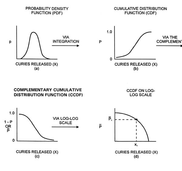
Most people are familiar with the concept of a bell-shaped curve as a way to convey confidence, or probability, in the value of a parameter, such as the number of curies released from an inventory of radionuclides. Such a curve tells how much of the probability is associated with intervals of curies released. This curve, called the probability density function, is the probability per unit interval of curies released. Of course such curves can be discrete, as in a histogram, or smooth, as in a continuous function (see Figure B.1[a]).
A more interesting question than the probability per release interval is referred to in risk assessment as "the exceedance question." This is the probability that the release will exceed a certain value (in the above example, exceed a certain number of curies of a particular radionuclide). This question can be answered by a summing, or integration operation, on the probability density function (Figure B.1[b]). The result of such a summation is called the cumulative distribution function. The complement—that is, one minus the parameter (here, the cumulative probability)—and the log-log scale are the additional steps taken to achieve the desired form (Figures B.1[c] and [d]). These steps result in a compact form for representing parameters that cover an extremely wide range of values.
Suppose, in the spirit of the triplet definition of risk, that a performance assessment has been conducted and a set of scenarios has been developed, each with its own probability density function of the number of curies of a particular radionuclide released. To cast the results in complementary cumulative form, the scenarios are structured in order of increasing release fractions and the probabilities are cumulated from the bottom to the top as a function of the different release fractions. Plotting the results on log-log graph paper generates a curve of the form shown in Figure B.1(d).
Figure B.1(d) does not represent reality, because it suggests that the outcome of a consequence is known with complete certainty. In practice, there are no absolutes; rather, there is significant uncertainty, starting with the uncertainties of the many individual inputs that are used to calculate a CCDF for a typical risk assessment. Thus, it is impossible to specify a single CCDF as the unambiguous outcome of a risk assessment. Instead, there are many possible CCDF curves (Figure B.2), each with its own likelihood of being correct. The spread of these CCDF curves provides a measure of the confidence with which the CCDF, for the consequence under consideration, can be estimated.
The uncertainty that gives rise to the CCDF curves in Figure B.2 is typically characterized by developing a probability distribution for each imprecisely known
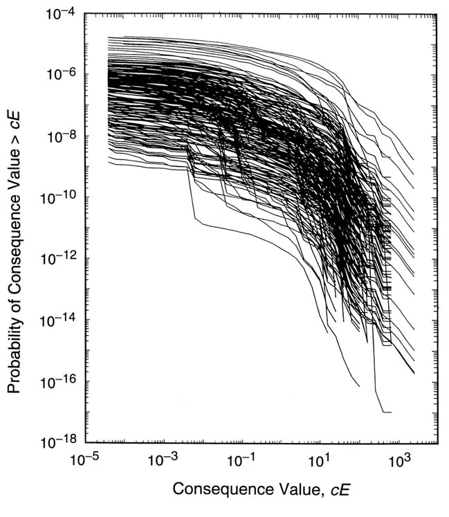
input used in the analysis. These distributions mathematically describe a degree of belief, based on all the available evidence (e.g., data, background knowledge, analyses, experiments, expert judgment), of the range and weight, in terms of likelihood, of the input values used in the analysis. An example of an input might be a distribution coefficient for a radionuclide transport calculation. Such distribution coefficients cannot be assigned a fixed number because of the uncertainty of what that number should be. Thus, the input has to be in the form of a probability distribution that expresses the analyst's state of knowledge about what the number should be. It tells a much fuller story than would be provided by a single number. The CCDF curves in Figure B.2 arise from the distributions assigned to the individual inputs.
The usual computational procedure is to generate a sample (e.g., random or Latin hypercube1) from the uncertain inputs according to their assigned distributions and then to construct one CCDF of the form appearing in Figure B.2 for each element of this sample. With this procedure, each CCDF is constructed from a set of input values (sometimes referred to as a "realization") that is consistent with all available information. Further, the assignment of distributions to individual inputs, and the propagation of these distributions through to the distribution of CCDF curves in Figure B.2, provide a representation of the uncertainty in the final outcome of the risk assessment, where this outcome is a CCDF. Put another way, the distribution of CCDF curves in Figure B.2 provides a measure of the confidence with which the outcome of the risk assessment can be estimated. A tight grouping of CCDF curves in Figure B.2 indicates a high confidence in the estimated location of the CCDF of interest; conversely, a wide spread in the CCDF curves indicates a low confidence in the estimated location of this CCDF.
Although Figure B.2 provides a complete summary of the distribution of CCDF curves obtained by propagating the uncertainty in the individual analysis inputs, it is rather crowded and difficult to read. A less crowded summary can be obtained by plotting the mean value and selected percentiles for each consequence value on the abscissa. For example, the mean plus the 5th, 50th (i.e., median), and 95th percentile values might be used (Figure B.3). The percentile curves then provide a measure of confidence as to the location of the exceedance probabilities for individual consequence values (e.g., there is a degree of belief probability of .9 that the exceedance probability for a particular consequence value is located between the 5th and 95th percentile curves). Further, the mean CCDF, obtained by vertically averaging the individual CCDF curves in Figure B.2, provides a measure of central tendency; the 50th percentile curve provides a related, but different, measure of central tendency. However, it is the distribution of CCDF curves that provides the overall measure of confidence that can be placed in the results of the risk assessment.
The distribution of CCDF curves in Figure B.2, and hence the mean and percentile curves in Figure B.3, are typically obtained by sampling-based techniques and therefore are approximate. However, if a robust sampling procedure is used, these results should show little variation from one sample to the next (Figure B.4). In concept, the mean and percentile curves in Figure B.3 can be specified uniquely by approximately defined integrals; in practice, these integrals have to be approximated by sampling-based techniques.

FIGURE B.3 Example summary curves derived from an estimated distribution of CCDF curves. The curves in this figure were obtained by calculating the mean and the indicated percentiles for each consequence value on the abscissa in Figure B.2. Source: Helton et al. (1991).

FIGURE B.4 Example of mean and percentile curves obtained with two independently generated samples for the results shown in Figure B.3. Source: Helton et al. (1991).


