From Scarcity to Visibility: Gender Differences in the Careers of Doctoral Scientists and Engineers (2001)

This chapter describes the data sets, variables, and methodology used for the analyses in the next five chapters. While the substantive chapters are largely self-contained, there is some critical information that was too detailed to include within each chapter. Accordingly, we encourage all readers to at least quickly review the information presented in this chapter.

The Ahern and Scott study examined career differences for women and men in mathematics, physics, chemistry, the biological sciences, psychology, the social sciences, languages and literature, and other humanities. Since the current study panel was charged with examining career outcomes for Ph.D.s only in science and engineering, we examined five broad fields:

• Mathematical Sciences: Mathematics, computer science, probability and statistics (including biometrics and biostatistics, psychometrics, econometrics, and social statistics), and other fields of mathematics.

• Physical Sciences: Astronomy, physics, chemistry, oceanography, and geosciences.

• Engineering: Biomedical engineering, chemical engineering, electrical engineering, industrial engineering, material sciences, and other fields of engineering.

• Life Sciences: Agriculture, biological sciences, and medical sciences.

• Social and Behavioral Sciences: Anthropology, economics, geography, political science, psychology, sociology, and other social and behavioral sciences.

Further details on these fields are given in Chapter 3 on Ph.D. production.

While our study examines both science and engineering, for simplicity we sometimes use the shorter term “science” rather than “science and engineering” to refer to the fields combined. Similarly, the term “scientists” is sometimes used as shorthand for “scientists and engineers,” and “scientist” for “scientist or engineer.”

Analyses are based on scientists and engineers who participated in the 1973, 1979, 1989, or 1995 Survey of Doctorate Recipients (NSF1973–1995). In this section we describe this survey, referred to as the SDR, along with other data sources that were used to supplement this key data source.

The scientists and engineers studied in our report were respondents to the Survey of Doctorate Recipients (NSF 1973–1995). Since 1973, with support from the National Science Foundation and other federal sponsors, the National Research Council (NRC) has conducted a biennial survey of doctoral scientists, engineers, and humanists who completed the Survey of Earned Doctorates (discussed on page 17). The sample for the SDR is stratified by year and broad field of Ph.D., gender, and other demographic variables. Responses to the survey are weighted to represent the science and engineering doctoral population. Sample weights are computed as the inverse of the probability of a case being selected from the population with adjustments based on the response rate from that stratum. Currently the SDR samples about 10 percent of the doctorates from U.S. universities who remain in the United States after they receive their degree. In earlier years of the survey, the sample was larger and included some individuals with doctorates from foreign institutions. In 1995 computer assisted telephone interviews (CATI) were used to increase the response rate and two weights were computed to account for differences

from earlier survey procedures. In our study the CATI weights were used. For technical details on the SDR, see NSF (1997).

For a given year, the SDR provides demographic characteristics and the current employment status of those with doctoral degrees awarded between 1930 and the present. Our analyses are based on data from four years of the SDK: 1973, 1979, 1989, and 1995. The 1973 survey was selected since it was the first year that data were available. The 1979 survey was used since this year was the primary data for the Ahern and Scott study. The 1989 survey provided information on changes in the decade since the 1979 survey. And, the 1995 survey was the most recent available when our analyses began.¹

The sample used for the SDR is based on the Survey of Earned Doctorates (NSF 1920–1995),² referred to as the SED. The SED is an annual survey that provides a nearly complete roster of recipients of doctoral degrees from American universities. For each respondent there is information on the year, field, and institution of bachelor’s, master’s, and doctoral degrees; elapsed and enrolled time from the bachelor’s to the doctorate; graduate support; plans for postgraduate employment; and the level of education of the respondent’s mother and father. The data from the SED become part of the Doctorate Records File (DRF), which is a virtually complete database on doctorate recipients from 1920 to the present. Since some of the information from the SED was not included in the SDR, data from the SED was merged with the SDR.

For the 1979 and 1989 panels of the SDR, data on publications were obtained by merging the SDR data with publication data from 1982 through 1992 from the Institute for Scientific Information (ISI). The ISI data covers over 16,000 international journals, books, and proceedings in the sciences, social sciences, and arts and humanities. In 1995, the SDR asked respondents to provide the number of publications they had since 1990. For the 1973 SDR, no data on publications were available.

Information on the quality of a scientist’s Ph.D. program was obtained by matching the SDR data to the NRC’s 1982 and 1995 studies of research-doctorate programs in engineering, humanities, life sciences, mathematics, physical sciences, and social/behavioral sciences in the United States (Goldberger, Maher, and Flattau 1995; Jones, Lindzey, and Coggeshall 1982). The scholarly quality of program faculty, also known as “reputational rating,” was used to measure the quality of the program from which the doctorate was received and the quality of the employing program in academia. This measure is the mean response to the survey after dropping the two highest and two lowest scores. The resulting means were converted to a scale from 0 to 5, with 0 denoting “Not sufficient for doctoral education” and 5 denoting “Distinguished.” The 1982 quality ratings for both the Ph.D. and employing program were matched with the 1973, 1979, and 1989 SDR data; the 1995 quality ratings were used for the 1995 employing program and for individuals who received their Ph.D.s between 1989 and 1994.

For each year of the SDR, data were analyzed for those with degrees from 1949 until the year of the survey. Those with degrees before 1949 were excluded due to the small number of cases. Table 2–1 is helpful for explaining the type of information provided by this research design. The left column indicates the year in which the SDR survey was conducted. The year of a respondent’s Ph.D. is listed at the top of the table; for simplicity the table only lists every fifth year. The body of the table contains the year since the Ph.D., referred to as the career year. The career year

is simply the year of the SDR survey minus the year in which a scientist received her Ph.D. For example, consider those with degrees in 1959 (the values have been underlined). For this cohort, we have information on their careers at four different times: when they were 14 years from the Ph.D. in 1973 (i.e., 1973–1959=14); 20 years from the degree in 1979; 30 years in 1989; and 36 years in 1995. Thinking of years since the Ph.D. as a scientist’s professional age (thus excluding any work activities before the Ph.D.), those with degrees in 1969 would have an age of 4 in 1973, 10 in 1979, 20 in 1989, and 26 in 1995.

We used this information to examine both changes that occur as a scientist ages through the career and changes in the climate of science over time.³ To illustrate the issues involved in using this type of panel data, consider a hypothetical analysis of promotion to the rank of full professor. By tracing the same cohort at different career stages, we can examine changes as a scientist ages. Consider scientists who received their degrees in 1959:

• Using the 1973 SDR, we can compute the percent who were full professors 14 years into their career; using the 1979 SDR we can compute the percent of this cohort who are full professors 20 years into the career; using the 1989 SDR, 30 years; and using the 1995 SDR, the percent 36 years after the Ph.D.

While the same scientists do not respond to each survey, the sample weights for those in each year’s sample are adjusted to represent the population as a whole. Accordingly, we interpret the sample data as if we are observing the same group of scientists as they age.

This design also allows us to compare the career outcomes of individuals who had the same career ages in different calendar years. For example:

• Table 2–1 shows that the 1959 cohort was 20 years from their Ph.D. in 1979, while the 1969 cohort was 20 years from the degree in 1989. By comparing the two groups, we can see the consequences of changes in the climate of science over the ten years from 1979 to 1989.

This example also illustrates the gaps in our data. We do not know the percent of the 1959 cohort who were full professors 15 years into the career since we do not have data collected in 1974. To fill in these gaps, we

use the method of synthetic cohorts. This idea can be explained by extending our example.

• Since we do not have data on the 1959 cohort 15 years after the Ph.D., we use data from the 1958 cohort collected in 1973, corresponding to 15 years after their degree. Data for the 1958 cohort in year 15 of the career are used to “synthesize” what would have happened to the 1959 cohort in their 15th year.

The degree to which a synthetic cohort is a good representation of the aging process depends on how close in time the cohorts are and the degree to which conditions facing scientists have changed. In later chapters, we are careful to qualify the degree to which this approach can be used to approximate changes over the course of the career.

While the same sample of scientists is not used for each year of the SDR, by chance some scientists are selected into the SDR sample in more than one year. We can use scientists who respond to two or more waves of the SDR to trace the same individuals at different times. Such analyses are used when there are a sufficient number of individuals responding to the same question in multiple years of the SDR.

This section describes the variables used in later chapters. We begin with the career outcomes and then consider the independent, antecedent, and control variables.

The report is organized around the metaphor of the pipeline (Berryman 1983; U.S. Congress, Office of Technology Assessment 1988:11–12), with Chapters 3 through 6 considering increasingly selective outcomes. Chapter 3 begins with the most general and inclusive outcome, obtaining the Ph.D. Women are less likely to obtain a doctorate, and those women who do not obtain a doctorate are necessarily excluded from consideration in Chapter 4, which examines labor force participation. Chapter 4 shows that female doctoral scientists are less likely than men to be in the fulltime labor force. Women who are not working full time are excluded from Chapter 5, where gender differences in sector of employment and primary activity are examined. Chapter 6 further limits analyses to those in the academic sector and within the chapter progressively restricts analyses to those with tenure-track positions, those with tenure, and finally those who are full professors. In reading later chapters, it is essential to

keep in mind that those scientists who are “filtered out” in earlier chapters, who are more likely to be women, are not considered in the next chapter. The specific outcomes considered in each chapter are as follows:

• Doctoral Degree Attainment. How has the percentage of doctoral degrees received by women changed since 1973?

For those with doctorates in science and engineering:

• Employment Status. Is the Ph.D. scientist employed full time, part time, unemployed, or underemployed?

For those in the full-time science and engineering labor force:

• Employment Sector. Does the scientist work in academia, business or industry, government, or the nonprofit sector?

• Primary Work Activity. Within each sector, is the scientist’s primary work activity teaching, basic research, applied research, development, management, or some other activity?

For scientists and engineers working in academia:

• Type of Institution. In what type of educational institution does a scientist work?

• Tenure-Track Positions. Does the scientist have a tenure-track position or is the scientist working off-track?

• Tenure. Is the scientist tenured?

• Rank. What is the faculty member’s academic rank?

• Productivity. How many publications does a scientist have?

Considering all full-time doctoral scientists and engineers:

• Salary. What is the respondent’s 12-month salary?

Male and female scientists and engineers differ in nearly every career outcome. To understand these gender differences, a wide variety of control variables were considered. These variables include:

• Field. Is the doctoral degree in engineering, mathematics, physical science, life science, or the social and behavioral sciences? In some analyses, medical science is split out from the broad field of the life sciences.

• Year of Survey, Year of Ph.D. and Career Year. As noted above, each of these measures of time is essential for understanding the changes in the status of women and men in science and engineering. Career year or career age is defined as years since the Ph.D., where employment prior to the Ph.D. is not counted.

• Race/Ethnicity. Is the respondent white, African American, Hispanic, or Asian?

• Citizenship. Is the respondent a U.S. citizen?

• Level of Parents’ Education. What is the highest level of education of the respondent’s mother and father?

• Marital Status. Is the respondent married?

• Children. Does the respondent have young children living at home?

• Type of Baccalaureate Institution. From what type of baccalaureate institution did the respondent obtain an undergraduate degree?

• HBCU. Did the respondent receive a baccalaureate degree from a Historically Black College or University (HBCU)?

• Women’s College. Did the respondent receive a baccalaureate degree from an institution belonging to the Women’s College Coalition?

• Time to Doctorate. How long did it take a scientist to complete the Ph.D.? Both time enrolled in graduate study and elapsed time from the undergraduate degree to the doctorate are considered.

• Type of Doctoral Institution. What is the Carnegie type of the

institution from which a respondent received her/his degree? Details on the Carnegie Classification are given below.

• Quality of Doctoral Department. What was the prestige of the doctoral department? This is measured on a scale ranging from 0 to 5, with 0 denoting “Not sufficient for doctoral education” and 5 denoting “Distinguished.” Further details are given below.

• Sources of Financial Support. What types of financial support did the respondent receive during graduate school? Did the respondent receive a research assistantship and/or teaching assistantship? How much debt was incurred during graduate school?

There is immense variation among the over 3,000 colleges and universities in the United States. To distinguish among these universities, we have used the well-known Carnegie Classification of Higher Education (Carnegie Commission on Higher Education 1973, 1976, 1987, 1994). The 1994 Carnegie Classification includes all colleges and universities in the United States that are degree-granting and accredited by an agency recognized by the U.S. Secretary of Education. For purposes of analysis, we simplified the classification to the following categories (the full classification is given in Appendix A).

• Research I institutions offer a full range of baccalaureate programs, are committed to graduate education through the doctorate degree, give high priority to research, and receive substantial federal support.

• Research II institutions are similar to Research I institutions, but receive a smaller amount of research support.

• Doctoral institutions include baccalaureate, master’s, and doctoral programs, but produce a smaller number of doctoral degrees in a more limited number of areas than Research I and II schools.

• Master’s institutions (also referred to as Comprehensive institutions) offer baccalaureate programs and usually have graduate education through the master’s degree. More than half of their baccalaureate degrees are awarded in two or more occupational or professional disciplines.

• Baccalaureate institutions (also known as Liberal Arts institutions) are primarily undergraduate colleges with a majority of degrees in arts and science fields.

• Medical institutions include medical and health related universities. We consider medical institutions to be Research I institutions except for some analyses of the life sciences.

• Engineering institutions include schools of engineering. We have classified these schools as Research I institutions.

• In addition, there are a variety of other types of institutions that include theological seminaries, bible colleges, law schools, business and management schools, schools of art, music, and design, teachers colleges, and corporate-sponsored institutions. Since these institutions employ only around 1 percent of our sample, divided proportionately between men and women, they have been excluded from the following analyses.

The Carnegie classifications are neither absolute nor invariant over time. First, within a given class there is substantial variation. For example, a university that barely meets the requirements to be a Research I university may be very similar to institutions at the upper range of Research II universities. Second, the Carnegie classifications was revised in 1976, 1987, and 1994 (Carnegie Foundation for the Advancement of Teaching 1973, 1976, 1987, 1994), leading to different classifications for the same institution over time. This could occur both because the institution changed, but also because of changes in the classification scheme. For example, a school that did not quite meet the criteria to be Research I in 1987 might satisfy those criteria in 1994 or may have grown into the new category. To avoid artifacts caused by institutions changing classifications, we used the classification of institutions from the 1994 report for all years of the SDR.

Data on the quality of the Ph.D. institution and the employing institution of the doctorates were obtained from the 1982 and 1995 NRC studies of research doctorate programs (Goldberger, Maher and Flattau 1995; Jones, Lindzey and Coggeshall 1982). Thirty-two fields were studied in 1982 and 41 fields in 1995. Programs within each field were evaluated on a range of objective and subjective measures. In our analyses, we used the rating for the “Quality of the Program Faculty.” On these ratings, scores less than 2 are classified as adequate programs; those from 2 through 2.99 as good programs; from 3 through 3.99 as strong; and those above 4 as distinguished.

The measure of quality used for the doctoral department depended on the year in which the degree was received. For degrees before 1988, ratings from the 1982 study were used. For those with degrees from 1989 to 1994, ratings were taken from the 1995 study. To assign quality measures to the Ph.D. program, a crosswalk was developed between the fields in the research-doctorate study and the Ph.D. fields in the DRF taxonomy. Data on the quality of the employing institution was based on the study that would most nearly represent the 1979, 1989, and 1995 employment data. For 1979 and 1989, the same crosswalk was used for employment as for the Ph.D. field since the SDR for those years used the same taxonomy

for field of employment as for Ph.D. field. For the 1995 SDR, field of employment was not collected, so we assumed that individuals worked in the field of their Ph.D. and assigned the quality rating of the Ph.D. program at their employing institution.

The Ahern and Scott (1981: Appendix B) study was based on a matched sample. This involved constructing triads of two men and one woman that matched as nearly as possible on selected background characteristics, such as education and years of experience. Matching was designed to control for the differences in characteristics between male and female Ph.D.s in the population. Comparisons of men to women from the matched sample allowed an assessment of the difference in outcomes after controlling (through matching) for key differences in background characteristics. For example, in comparing the academic rank of women to men, it was possible to show gender differences after controlling for those characteristics that were used to match the samples. The advantage of this approach was that once the matching was done, comparisons were simple since descriptive statistics and cross-tabulations could be used.

There are two limitations of matching that justify an alternative strategy. First, men and women can only be matched on a few characteristics due to limitations in the number of cases that are available. For example, in comparing rank it is not possible to control through matching for the productivity of the scientist or the quality of the employing department. Second, to the degree that men and women in the population of scientists and engineers differ on the variables used to match, matching resulted in a sample that was not representative of the population. Since male and female scientists differ on the characteristics used for matching, statistics based on the matched sample should not be used to represent the distribution of characteristics in the population. We note, however, that some readers of the Ahern and Scott report appear to have incorrectly used the study’s results to generalize to the populations responding to the 1973 and 1979 SDRs.

In response to these concerns, we used statistical analyses of all cases in selected years of the SDR, rather than a matched subsample. Consequently, the descriptive statistics reported can be taken as being representative of the population of scientists (to the extent that the SDR is representative, of course). Moreover, this approach allowed us to introduce a larger number of controls as independent variables in regression models. The greatest cost of this strategy is that the analyses and interpretation of

results were more complicated than those required for the earlier study. These methods are discussed below.

The regressions are not used as causal models; rather they are sophisticated descriptions of the association between background characteristics and career outcomes. For example, if women with children are more likely to leave science, this is not conclusive evidence that the cause of these women leaving science is having children. Drawing such conclusions requires far more detailed analyses based on complete career histories and the measurement of variables that were not available. Further, the panel recognized that: 1) we did not have a simple random sample; 2) response rates to the surveys varied from 79 percent of those contacted in 1973, to 71 percent in 1979, to 63 percent in 1989, and 85 in 1995; 3) not all variables that we wanted were available; and 4) missing data were a problem for some variables (especially race and ethnic origin). Still, we firmly believe that our analyses provide useful and accurate information about differences in the careers of male and female scientists.

Loglinear regression was used to analyze salaries, while logit analysis was used for binary and nominal outcomes. These methods are now described.

Salary was treated as a continuous variable, which allowed the use of multiple regression. Data from 1973, 1979, and 1989 were converted to 1995 dollars using adjustment factors for inflation from the U.S. Census Bureau (1999). Given the skewed nature of the salary distribution, we used the standard practice of taking the natural log before estimating the regression. To explain the model used, we assume only three independent variables, although many more were included in the actual regressions. Let y indicate salary and let x₁ through x₃ be the independent variables, which can be either binary or continuous. The effects of the independent variables were allowed to vary by sex. Consequently, the estimated model was:

Given the loglinear specification, the effects of variables can be interpreted by transforming the β coefficients. Consider the effect of x₁ for

women. The transformation exp(β_1,W) is the factor change in the expected value of y for a unit increase in x₁, holding all other variables constant. Or, 100[exp(β_1,W)—1] can be interpreted as the percentage change in salary y for a unit increase in x₁, holding all other variables constant. For example, if the coefficient for the quality of the doctoral program was 0.049, then 100[exp(.049)—1]=5.02 indicates that for every unit increase in the prestige of the doctoral department, salary is expected to increase by 5 percent, controlling for all other variables.

We also compared men and women by computing predicted salaries under various conditions. Since the model is loglinear regression, we could not compute the expected value as:

Rather, we need to estimate:

To compute this quantity, Duan (1983) proposed a nonparametric smearing estimator which he described as “a low-premium insurance policy against departures” from the usual assumption regarding the distribution of the errors. If e_i is the ordinary least squares residual, then define:

The smearing estimate, which is a consistent estimator of the expected outcome, was used for computing predicted salaries:

For binary and nominal outcomes, the logit model was used. The logit model specifies a nonlinear relationship between the probability that some event occurs and a set of independent variables. To interpret the effect of an independent variable, we compute the change in the predicted probability of some outcome when one of the independent variables changes by a given amount. The levels of all other variables are held

constant at their mean or at some level that is substantively interesting. To explain this method, we consider the case of a binary outcome. Further details and generalization to nominal outcomes can be found in Long (1997).

Let y be a dummy variable equal to 1 if an event occurred and 0 if not. For example, y=1 if a scientist has tenure and y=0 if not. Let x₁ through x₃ be the independent variables, which can be either binary or continuous. The logit model uses the x’s to predict the probability that y=1 according to the equation:

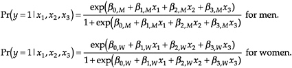
These equations describe a nonlinear relationship between the x’s and the outcome probabilities. The problem in presenting results from the logit model is that the expected change in the probability for a unit change in a variable differs depending on the current level of all variables in the model.

To summarize the effect of a variable, we examined how a unit change in a variable affected the outcome probability when all variables were held constant, usually at their mean. For a continuous variable x_c, we computed:

This is simply the difference in the predicted probability when x_c moves from .5 below its mean to .5 above its mean, holding all other variables at their means. In the text, we interpreted this as: when x_c changes by one unit, the probability of the event changes by ∆p_c. For binary independent variables, we computed the effect of a change from 0 to 1:

In some cases we focused on predicted probabilities and changes in predicted probabilities at levels of the variables other than the mean. For example, in Chapter 6 we were interested in the predicted probability of being a full professor. Given that promotion to full professor rarely occurs early in the career, we computed the predicted probability holding years of experience constant at 15 years while other variables were held constant at their mean.