Motion, Control, and Geometry: Proceedings of a Symposium (1997)

Richard M. Murray

Department of Control and Dynamical Systems and Department of Mechanical Engineering California Institute of Technology

The earliest robots consisted of simple electromechanical devices that could be programmed to perform a limited set of tasks. They were a cross between numerically controlled milling machines and the master-slave teleoperators developed for handling radioactive material. These robots are the

precursors to the automated machines used for painting, welding, and pick-and-place operations in today's factories. For these types of automation and manufacturing tasks, the complexity of the robot can be minimized since the workspace of the robot can be carefully controlled and the robots are not required to perform particularly dextrous manipulation of objects. However, many future applications of robotics are moving toward more autonomous operation in highly uncertain environments. The robots being developed for these applications are increasingly complex and have a high degree of interaction with their environment.

Examples of the next generation of robots range from miniature robots for medical inspection and manipulation inside the human body to mobile robots for exploration in hazardous and remote environments. All these robots will require sensing, actuation, and computational capabilities that were unheard of just a few years ago. However, as we seek to design robots that can act with increasing autonomy, we move closer to endowing robots with human-like capabilities. And we begin to become limited by our own ability to understand and analyze the highly complex systems that we are trying to control.

As the complexity of robots increases, so does the importance of abstraction and theory in understanding and analyzing robot motion. One approach that has begun to yield new insights is the use of differential geometry, in the context of both geometric mechanics and nonlinear control theory. Two specific areas where progress is being made are locomotion and manipulation in robot systems.

Locomotion is defined as the act of moving from one place to another. For robots, there are several mechanisms by which this movement can occur. The use of wheels and of legs are the two traditional methods, but other possibilities, such as undulatory gaits in snake-like robots, have also been proposed and implemented. Each of these mechanisms has certain advantages over the others, but all of them fundamentally involve interaction with their environment. Locomotion is achieved by pushing, sliding, rolling, or a combination of all of these.

Robotic manipulation involves motion of an object rather than motion of the robot itself. The prototypical example is a multifingered hand manipulating a grasped object. Once again, the fundamental mechanisms that govern motion involve pushing, rolling, and sliding. The motion of a set of fingers grasping an object is constrained in much the same way as the motion of a legged robot is constrained by the contacts between its feet and the ground. Indeed, many of the tools that are used to analyze manipulation and grasping problems are easily adapted to analyze locomotion.

The most basic problem in all locomotion and manipulation systems is to devise a method for generating and controlling motion between one configuration and another. The common feature is that motion of the robot is constrained by its interactions with the environment. For example, in wheeled mobile robots the wheels must roll in the direction in which they are pointing and they must not slide sideways. In grasping, the motion of the fingers is constrained by the object being held in the grasp: motion of one finger affects the others since forces are transmitted between the fingers by the object. Even in legged robots, one usually assumes that the feet do not slip on the ground, allowing the robot to propel itself. These constraints on the motion of the system are the defining features for how locomotion and manipulation work in these systems.

Furthermore, in most locomotion and manipulation systems, the range of the actuators is small, while the desired net motion for the system may be large. A good example of this is using your fingers to screw in a light bulb: repeated grasping and twisting of the bulb is required in order to fully insert it into the socket. A large motion of the light bulb (multiple revolutions) is accomplished by repeated (i.e., periodic) small motions in your fingers.

In this paper we consider locomotion and manipulation using the notion of geometric phases as a central theme. Intuitively, geometric phases relate the motion of one parameter describing the configuration of a system to other parameters that undergo periodic motion. A simple example of geometric phase is the motion of an automobile performing a parallel parking maneuver. By moving the car backwards and forwards and turning the steering wheel in a periodic fashion, a driver is able to achieve a net sideways motion of the car even though the car cannot move sideways directly. This net sideways motion is the geometric phase associated with this choice of the car velocity and steering wheel angle.

The role of geometric phases as a means of analyzing locomotion is a relatively new perspective. One of the earliest works is that of Shapere and Wilczek (1989), who studied the motion of paramecia swimming in a highly viscous fluid. They show that periodic variations in the shape of an organism can be used to achieve net forward motion. This is very reminiscent of the type of motion present in parallel parking and this similarity can be made precise by using geometric phases.

There has also been an increased interest in the use of geometric phases for understanding motion in other biological systems, such as snakes and insects. Here again, periodic changes in one set of variables, which describe the shape of the system, are used to obtain net motion. The phasing of the inputs plays a central role, generating different gaits for achieving different types of motion. The interpretation of locomotion in terms of geometric phases is still far from complete, but it is providing a unifying view of locomotion and manipulation that has already yielded new insights and has impact on several challenging applications.

Locomotion involves movement of a mechanical system by appropriate application of forces on the robot. These forces can arise in several ways, depending on the means of locomotion used. The simplest form of locomotion is to apply the forces directly, as is done in a spacecraft, where high-energy mass is ejected in the direction opposite to the desired motion. A similar technique is the use of jet engines on modem aircraft.

For ground-based systems, a much more common means of locomotion is the use of forces of constraint between a robot and its environment. For example, a wheeled mobile robot exerts forces by applying a torque to its drive wheels. These wheels are touching the ground and, in the presence of sufficient friction, are constrained so as not to slip along the ground. This constraint is enforced by the application of internal forces, which cause a net force on the robot that propels it forward. If no constraints existed between the robot and the ground, then the robot would just spin its wheels. Similarly, for legged and snake robots, the parts of the robots in contact with the environment are used to exert net forces on the robot. In fact, for a large class of robotic systems we can view constraints as the basis for locomotion.

A second common feature in robot locomotion is the notion of base (or internal) variables versus fiber (or group) variables. Base variables describe the geometry and shape of the robot, while fiber variables describe its configuration relative to its environment. For example, in a snake robot the fiber variables might be the position and orientation of a coordinate frame fixed to the robot's body, while the base variables would be the angles that describe the overall shape of the robot. These base and fiber

variables are coupled by the constraints acting on the robot. Hence, by making changes in the base variables, it is possible to effect changes in the fiber variables.

In this paper we concentrate on a particular type of constraint on the configuration variables of the robot, known as a Pfaffian constraint. Consider a mechanical system with configuration space and configuration . A Pfaffian constraint restricts the motion of the system according to the equation

where ω(q) is a row vector that gives the direction in which motion is not allowed. Pfaffian constraints arise naturally in wheeled mobile robots: they model the ability of a wheel to roll along the ground and spin about its vertical axis but not slide sideways. Pfaffian constraints typically do not provide a complete model of the interaction with the environment, since frictional forces are present in both rolling and spinning, but they do capture the basic behavior of the system.

As an example, consider a simple kinematic model of an automobile, as shown in Figure 3.1. The constraints are derived by assuming that the front and rear wheels can roll and spin (about the center of the axle) but not slide. Let denote the configuration of the car, parameterized by the xy location of the center of the rear axle, the angle of the car body with respect to the horizontal, Θ, and the steering angle with respect to the car body, Φ. To simplify the derivation, we model the front and rear pairs of wheels as single wheels at the midpoints of the axles. The constraints for the front and rear wheels are formed by setting the sideways velocity of the wheels to be zero. A simple calculation shows that the Pfaffian constraints are given by

FIGURE 3.1 Kinematic model of an automobile. The configuration of the car is determined by the Cartesian location of the back wheels, the angle the car makes with the horizontal, and the steering wheel angle relative to the car body. The two inputs are the velocity of the rear wheels and the steering velocity.

For simplicity we take l = 1 in the sequel.

To study the motion of a system subject to a set of Pfaffian constraints {ω₁,. . .,ω_k, it is convenient to convert the problem to a control problem. Roughly speaking, we would like to shift our viewpoint from describing the directions in which the system cannot move to describing those in which it can. Formally, we choose a basis for the right null space of the constraints, denoted by . The locomotion problem can be restated as finding an input function, , such that the control system

achieves a desired motion. The g_i's can be regarded as vector fields on , describing the allowable motion of the system. This type of control system is called a driftless control system since setting the inputs to zero stops the motion of the system.

For the kinematic car, this conversion yields the control system

For this choice of vector fields, u₁ corresponds to the forward velocity of the rear wheels of the car, and u₂ corresponds to the velocity of the steering wheel.

The first question one must consider when analyzing a control system is whether the system is controllable. That is, given an initial state x_i and a final state x_f, does there exist a choice of inputs u that will steer the system from one state to the other? A geometric interpretation of this question can be formulated by studying the properties of the vector fields that define the control system. A set of vector fields which is not controllable is shown in Figure 3.2. For these vector fields, there exists a surface whose tangent space contains the span of the vector fields: Hence, any motion of the system is necessarily restricted to this surface and it is not possible to move to an arbitrary point in the configuration space (only to other points on the same surface).

To test whether a set of vector fields are tangent to some surface, we make use of a special type of motion called a Lie bracket motion . Roughly, the idea is to choose two vector fields, say g_l and g₂, and construct an infinitesimal motion by first flowing along g₁ for ε seconds, then flowing along g₂ for ε seconds, and then flowing backwards along g₁ for ε seconds and backwards along g₁ for ε seconds. This motion is illustrated in Figure 3.3. A simple Taylor series argument shows that the net motion given by this strategy is

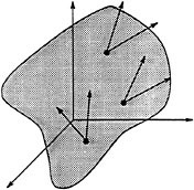
FIGURE 3.2 A set of vector fields that are tangent to a hypersurface in the configuration space. The system described by this set of vector fields is not controllable since motion is restricted to a hypersurface.

FIGURE 3.3 A Lie bracket motion.

(See Murray et al., 1994, pp. 323-324 for a derivation.) Motivated by this calculation, we define the Lie bracket of two vector fields g₁ and g₂ as

The Lie bracket of g₁ and g₂ describes the infinitesimal motion due to cycling between the inputs corresponding to g₁ and g₂.

The Lie bracket between two vector fields gives a potentially new direction in which we can move. In particular, if [g₁,g₂ ] is not in the span of g₁ and g₂, then it is not possible for g₁ and g₂ to be locally tangent to a two-dimensional surface, since we could move off such a surface by executing a Lie bracket motion. Furthermore, from a controllability point of view we can treat g₃ = [g₁,g₂] as a new direction in which we are free to move, and we can look at higher order bracket motions involving g₃. A fundamental result, proven in the 1940s by the German mathematician W.-L. Chow (1940), is the central result in controllability for control systems of this type. Let be the set of all directions that can be achieved by the input vector or repeated Lie brackets. That is,

Theorem 1 (Chow) A driftless control system is controllable in a neighborhood of

We can verify that the kinematic car satisfies Chow's theorem by direct calculation. The input vector fields are given by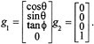

We call g₁ the drive vector field, corresponding to the motion commanded by the gas pedal, and g₂ the steer vector field, corresponding to the motion of the steering wheel.¹ The Lie bracket between the drive and steer vector fields turns out to be

We call g₃ the wriggle vector field; it gives infinitesimal rotation of the car about the center of the rear wheels. Finally, we compute the Lie bracket between drive and wriggle, which yields

This vector field is called the slide vector field since it corresponds to motion perpendicular to the direction in which the car is pointing.

The four vector fields g₁, g₂, g₃, and g₄ span as long as (at which point g₁ is not defined). By Chow's theorem this means that we can steer between any two configurations by an appropriate choice of input.

What Chow's theorem does not tell us is how to synthesize an input that causes the car to move to a given location. Of course, humans are very good at synthesizing trajectories for automobiles, but for more complicated situations (such as backing a truck with two or three trailers into a loading dock), the solution to the locomotion problem is not so intuitive.

One method for synthesizing trajectories is to use the Lie bracket motions described earlier. The problem is that these motions are only piecewise smooth in the inputs (a problem here since we are commanding velocities) and they only generate infinitesimal motions. A partial solution to these issues was explored in Murray and Sastry (1993), where we suggested the use of sinusoids to steer control systems of this form. The basic idea was to use sinusoids at integrally related frequencies to generate motion in the Lie bracket directions. In essence, one replaces the squares of a Lie bracket motion with circles. By varying the relative frequencies of the inputs, motion corresponding to different combinations of brackets between the inputs can be obtained. These calculations were motivated by results of Brockett (1981), who showed that under certain conditions these types of inputs are actually optimal.

An example of this type of motion is shown in Figure 3.4. The input, shown in the lower right, consists of a sequence of sinusoidal input segments with different frequencies. The first part of the path, labeled A, drives x and to their desired values using a constant input. These are the states controlled directly by the inputs, so no periodic motion is needed.

The second portion, labeled B, uses a sine and cosine to drive θ while bringing the other two states back to their desired values. Thus, choosing u₁ = a sin t and u₂ = b cos t gives motion in the wriggle direction, [g₁,g₁]. By choosing a and b properly, we can control the net change in orientation. However, a careful examination of the motion reveals that some motion also occurs in the y direction. This is due to the higher order terms that appear in the expression for a Lie bracket motion. However, the input directions, x and , return to their original values.

The last step, labeled C, uses the inputs u₁ = a sin t and u₂= b sin 2 t to steer y to the desired value and returns the other states back to their correct values. This choice of inputs moves the car back and forth once while rotating the steering wheel twice in the proper phase. It generates motion in the bracket direction corresponding to slide, g₄ = [g₁[g₁,g₂]]. Notice that the Lie bracket expression contains two copies of g₁ and one copy of g₂, while the inputs move twice in u₂ versus once in u₁.

FIGURE 3.4 Motion of a kinematic car. The trajectory shown is a sample path that moves the car form (x, y,θ,Φ) = (5,1, 0.05,1) to (0, 0.5, 0, 0). The first three figures show the states versus x, and the boom right graphs show the inputs as functions of time. Repented, by permission, form Murray and Sastry, 1993. Copyright © 1993 by Institute of Electrical and Electronics Engineer.

The Lissajous figures obtained from the phase portraits of the different variables are quite instructive. Consider the part of the curve labeled C. The upper left plot contains the Lissajous figure for x, (two loops); the lower left plot is the corresponding figure for x, Θ (one loop); and the open curve in x,y shows the increment in the y variable. The interesting implication here is that the Lie bracket motions correspond to rectification of harmonic periodic motions of the driving vector fields, and the harmonic relations are determined by the order of the Lie bracket corresponding to the desired direction of motion.

It is instructive to reinterpret this example in terms of geometric phases. To do this, we rewrite the equations of motion for the system as

Note that the right-hand set of equations have the form of a set of Pfaffian constraints. One can directly verify that these equations describe the motion of the system by identifying (s₁, s₂, s₃) with (x, y,θ) and

of u₁ and u₂ with the driving, steering, and velocity. The variable r₁ represents the (signed) distance traveled by the car and r₂ the angle of the steering wheel.

The decomposition of the problem into a set of independent variables, , and dependent variables, , is an example of a fiber bundle decomposition of the system. We call the base variables and we call the fiber variables. Looking back at Figure 3.4, we see that the motion of the fiber variables in segments B and C is obtained by using closed loops in the base variables. The amount of motion in the fiber variables, due to a trajectory in the base variables, is the geometric phase associated with the path in the base space. Parallel parking corresponds to a phase shift in the y direction, while making a U-turn corresponds to a phase shift in the θ direction (sometimes combined with y).

The trajectories shown in Figure 3.4 show how geometric phases can be used to understand car parking, but they are not very good examples of parallel parking maneuvers. In fact, it is possible to get much better trajectories for this system by using some obvious tricks, such as using the sum of a set of sinusoids instead of applying simple periodic inputs in a piecewise fashion. One can even solve for the optimal trajectories in simple examples such as this one. Reeds and Schepp (1990) showed that the optimal trajectory between any two configurations can be obtained by following a path comprising up to five segments consisting of either straight, hard left, or hard right driving in either forward or reverse. Furthermore, they were able to show that no more than two backups are required and that only 48 different input patterns are needed to construct minimum length paths (this number has since been reduced to 46 by Sussmann and Tang, 1991).

A somewhat more complicated example of geometric phases occurs in the area of dextrous manipulation using multifingered robot hands. Here the basic issues involve the use of phases for repositioning the fingers of a hand without removing the fingers from the object. In fact, one is usually more interested in making sure that geometric phase is not generated, so that periodic motions of the object cause the fingers to return to their original positions. We start by discussing the repositioning problem and then make some brief comments about generating cyclic motions.

Consider the grasping control problem with rolling contacts, such as the system shown in Figure 3.5. Assuming that the fingers roll without slipping on the surface of the object (a very useful assumption to enforce, since control of sliding is very tricky), the constraints on the system can be described by a set of equations of the form

(3.2)

where θ is the vector of finger joint angles and x specifies the position and orientation of the grasped object. In the robotics literature, J_h is called the hand Jacobian and G is the grasp map (see Murray et al., 1994, for a detailed discussion).

FIGURE 3.5 Multifingered hand grasping an object. Reprinted with permission from Murray et al., 1994. Copyright © 1994 by CRC Press, Boca Raton, Florida.

A detailed calculation of the hand Jacobian and grasp map is quite involved and makes use of a large amount of specialized machinery. However, the basic idea behind the grasp constraint is quite straightforward: the left-hand side of equation 3.2 is the vector of fingertip contact velocities for the robot hand, expressed in an appropriate frame of reference. The right-hand side of equation 3.2 is the vector of velocities for the contact points on the object, expressed in the same frame of reference. The condition that the fingers roll without slipping is obtained by equating these sets of velocities.

If the fingers of a grasp have sufficient dexterity, they can follow any motion of the object without slipping. A grasp of this type is called a manipulable grasp. For manipulable grasps, any object velocity can be accommodated by some finger velocity vector θ. However, the vector θ may not be unique in the case that the null space of J_h—that is, the set of vectors that J_h maps to the zero vector—is nontrivial. This situation corresponds to the existence of internal motions of the fingers that do not affect the motion of the object. If we let u₁ be an input that controls the velocity of the object and let u₂ parameterize the internal motions, then equation 3.2 can be written as

(3.3)

where is the right pseudo-inverse of J_h and K is a matrix whose columns span the null space of J_h.

Equation 3.3 describes the grasp kinematics as a control system. The input u₁ describes the motion of the object, whose position is given by x. The effect of u₁ on θ describes how the fingers must move in order to maintain contact with the object. If the fingers have any extra degrees of freedom, u₂ can be used to control the internal motions that affect the shape of the fingers but leave the object

position unchanged. The dynamic finger repositioning problem is to steer the system from an initial configuration (θ₀,x₀) to a desired final configuration (θ_f,x_f). The explicit location of the fingertip on the object at the initial and final configurations can be found by solving the forward kinematics of the system.

The general case of finding u₁ (t) and u₂ (t) such that the object and the fingers move from an initial to final position (while maintaining contact) can be very difficult. A special case is when the object position is kept fixed by setting u₁ at zero. If there are still sufficient degrees of freedom available for the fingers to roll on the object, then the internal motions parameterized by u₂ can be used to move the fingers individually around on the object. With the object position held fixed, each of the fingers can be controlled individually without regard to the motion of the others, simplifying the problem somewhat.

An example of such a path moving a spherical fingertip down the side of a planar object is shown in Figure 3.6. In this figure we consider the motion of a finger with a spherical tip on a rectangular object. The plots show trajectories that move a finger down the side of the object. The location of the contact on the finger is unchanged, as shown in the right graph, which plots the finger contact configurations (u_f, ν_f), while the location of the contact on the face of the object (u₀,ν₀) undergoes a displacement in the ν₀ direction.

In addition to describing how the fingers can be repositioned on the object without releasing contact, geometric phases can also be used to understand when control laws keep the fingers from drifting, in case this is not desired. Imagine, for example, performing a complicated manipulation of an object. Depending on the geometry of the object and fingers, it is possible that the object might return to its starting configuration while the fingers would have shifted to a new location. In many cases we are interested in choosing control laws to ensure that this does not happen. Thus, we want to control the fingers in such a way that there is no geometric phase associated with any closed loop motions of the controls.

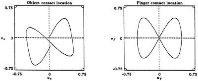
FIGURE 3.6 Steering applied to the multifingered hand shown in Figure 3.5. The left plot shows the location of the contact point on the object, and the right plot shows the corresponding contact point on the finger. The object contact moves down and slightly to the right, so the object is shifted slightly in the grasp after executing the steering maneuver.

A controller that always returns the fingers to their original configuration when the object returns to its original configuration is said to be cyclic. The same type of problem can occur in resolving motion in redundant robots, and has been studied a great deal in that context. In terms of the point of view described in this paper, the work of Shamir and Yomdin (1988) gives necessary and sufficient conditions in terms of Lie brackets that guarantee that a controller is cyclic. The same basic ideas can be used in the grasping case.

Using the kinematics described in equation 3.3, the input u₁ describes the motion of the object. To make the overall controller cyclic, we must choose u₂ so that any cyclic motion of u₁ gives a cyclic motion in θ. Thus, we wish to choose a feedback law u₂ = α (x,θ) such that the geometric phase associated with u₁ is always zero.

While dynamic finger repositioning provides a direct connection between geometric phases and manipulation, the basic ideas behind phases are present in other types of manipulation as well. Consider the problem of inserting a light bulb into a threaded hole using your fingers. One way to do this would be to grab the bulb and then walk around in circles to insert it. This obviously requires a large workspace and is completely inappropriate for manipulation inside a cluttered environment (like the inside of a refrigerator).

A much more natural way to insert the bulb is to rotate your fingers, release the bulb, and then move your fingers back to perform another rotation. If we treat ''twisting'' and "grasp/release" as inputs, then this type of motion corresponds exactly to a Lie bracket motion where the bracket direction corresponds to the motion of the bulb into the socket. The description of this problem does not quite fit into the differential framework described above without some modification of the underlying mathematics, but the basic notion of a Lie bracket motion is still present.

Another example along these lines is using a (miniature) multifingered hand for sewing stitches in tissue. To understand how such a hand should be designed and how such a task might be accomplished, we can use the tools from geometric phases to guide our insights and uncover the fundamental principles that govern the behavior of the system. Since these systems tend to be highly complex, it is important to understand the essential geometry of the system and its role in satisfying the overall task. The implications of some of these ideas in areas such as planetary exploration and medicine are discussed in the next section.

We now discuss two specific applications of the techniques outlined above to existing and future robotic systems.

In 1996 NASA is scheduled to launch a spacecraft to Mars containing the Microrover Flight Experiment MFEX (Pivirotto, 1993). A major part of the mission consists of landing a semiautonomous rover on the surface of Mars and using the rover to analyze soil and rock samples on the Martian surface.

Due in part to funding cuts in the program, the size of the rover has been reduced from an initial mass of 800-1000 kg to a "mini" or "micro" rover in the 5-50 kg range.

The starting point for the MFEX rover design is the Rocky IV rover pictured in Figure 3.7. Rocky IV has a mass of 7.2 kg and is approximately 60 cm in length. It uses a novel "rocker-bogie" design for the wheels, which allows it to climb over obstacles that are as much as 50 percent larger than the wheel diameter. Rocky IV is equipped with a color video camera and numerous proximity sensors. The flight version of the rover will also be equipped with an alpha proton X-ray spectrometer (AXPS), to be used to analyze the composition of Martian soil and rocks.

The three primary goals of the MFEX rover mission are to complete a set of technology experiments in at least one soil type, complete an AXPS measurement on at least one rock with a video image of that rock, and take at least one full image of the lander. When these goals are met, the rover will complete additional experiments on different soil and rock types and attempt to take two more pictures of the lander, giving a complete view from all sides.

Figure 3.7 Rocky IV rover. Used by permission of the Jet Propulsion Laboratory, California Institute of Technology, Pasadena, California.

The basic mode of operation for the Mars rover mission involves humans providing overall planning and guidance while the rover itself will be responsible for low-level navigation and control. This level of autonomy in the control of the rover is necessitated by two factors: communication delays to Mars and limited communications bandwidth. The round-trip travel time for a signal to Mars can

range from approximately 10 minutes to as long as 40 minutes. This makes direct teleoperation of the rover impossible. Furthermore, the communications bandwidth of the lander is limited to approximately 4 megabits/day, or the equivalent of 10 bytes every 1.7 seconds, and can only be sustained while Earth is visible from the lander sight.

Because of these communications limitations, the Mars rover will be given commands once per day describing a sequence of actions to be carried out. Onboard computation will be used to provide low-level trajectory tracking and to ensure obstacle avoidance. Due to power constraints on the rover and the need to use flight-qualified hardware, the amount of computational power onboard the rover is quite low. Current earth-based experiments employ an 8-bit microprocessor capable of performing only 1 million operations per second and containing less than 40K of memory. Behavioral control is being explored as a means of implementing the controller and has shown good reliability in autonomous navigation and manipulation tasks in both indoor and outdoor rough-terrain environments (Gat et al., 1994).

Path planning for the Mars rover involves finding paths that satisfy the basic kinematics of the rover and also avoid obstacles. To a rough degree of approximation, the constraints on the rover can be described by a set of Pfaffian constraints and hence the geometric machinery described above can be used to understand the vehicle motion and to plan maneuvers. Examples of path planners for mobile robots in the presence of obstacles can be found in Latombe (1991) and Laumond et al. (1994).

Future Mars missions are expected to include a sample and return scenario, in which a soil sample from Mars will be returned to the lander for further analysis. Since the lander can house much larger and heavier measurement apparatus than the rover can, returning a soil sample to the lander allows much more detailed experiments to be run. In returning to the lander, the rover must accurately position itself to dock with the lander. This must be done in the presence of unknown terrain and with a reasonably high degree of precision.

One approach to this problem is the use of controllers that use real-time feedback to guide the rover to the docking bay. Stabilization of constrained systems of this type turns out to be a challenging theoretical problem that has received a large amount of attention in the controls community over the past several years (see M'Closkey and Murray, 1994, for a recent list of papers and experimental results in active stabilization). These results have relied heavily on the geometric point of view, which has evolved over the past few years and will no doubt continue to make use of these tools.

One of the exciting applications of robotic manipulation and locomotion is in medicine, particularly in minimally invasive surgery. Over the past ten years, the use of minimally invasive surgical techniques has increased dramatically in the U.S. and abroad. These techniques offer several advantages over conventional surgery, including reduced hospital stays after an operation and decreased risk of infection and other complications.

A typical minimally invasive surgical operation is a laparoscopic cholecystectomy (gall bladder removal). In this procedure, a doctor removes the gall bladder through several small incisions in the patient's abdomen. One of the incisions is used to insert a tube that inflates the abdominal cavity with gas, while the other incisions are used to insert medical instruments. The gall bladder is removed by cutting it with a pair of scissors and extracting it through one of the incisions.

Gall bladder removal is one of the most common surgeries performed in the United States. Ten to fifteen years ago, the percentage of such surgeries that were done using minimally invasive techniques was negligible. However, with new techniques and new medical instruments, the use of minimally invasive techniques has surged, and this is by far the most common method currently in use for gall bladder removal.

Another minimally invasive surgical technique is the use of an endoscope for inspection and removal of tissue or polyps from the gastrointestinal tract. One example is an endoscopic polypectomy. In this procedure, a flexible endoscope is maneuvered near a polyp on the interior of the colon. Using a video display connected to a camera at the end of the endoscope (via fiber optics), the surgeon is able to snare the polyp and cut it off with electrocautery while drawing the snare closed.

While the use of minimally invasive techniques has progressed rapidly, it is currently limited by several factors. Among them is the limited dexterity of the tools used by the surgeons and the large portions of the body that cannot be reached with an endoscope or laparoscope. One of the applications of the work described here is toward extending the abilities of surgeons in these directions.

Researchers at the University of California-Berkeley, Harvard, and other institutions are working to develop a teleoperative surgical workstation, which would allow surgeons more dexterity and ease of use than current minimally invasive technology (Cohen et al., 1994). These researchers are focusing on a number of different problems, including the design, fabrication, and control of miniature robotic hands and the use of instrumented data gloves to allow the surgeon to control the hands in a natural way. A photograph of one of the hands that has been fabricated is shown in Figure 3.8.

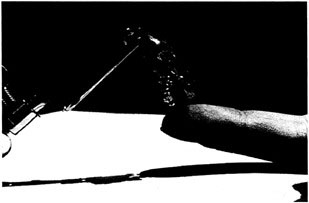
Figure 3.8 Three-fingered laparoscopic manipulator designed for tendon actuation (tendons omitted for clarity). The manipulator is shown in a 10 mm diameter laparoscopic trocar. Reprinted with permission from Michael Cohn, University of California-Berkeley.

The design and control of these complicated machines require a thorough understanding of the basic mechanisms that are present in manipulation tasks. A fairly simple miniature hand such as the one shown in Figure 3.8 might have up to 9 degrees of freedom, which, when combined with the dynamics of the object, can give a phase space with as many as 24 states (configurations plus velocities). The

dynamics for such a system cannot be easily studied without understanding the basic structure that the dynamics inherit from the specific manipulation problem under consideration.

A second area of research in medical robotics is the development of small locomotion robots capable of navigation and inspection in the gastrointestinal tract. J. Burdick and his students at Caltech have built several prototype devices for locomotion inside an intestine, and clinical trials on pigs are in development (Burdick, J.W. and B. Slatkin, 1994, personal communication). The motion of their devices relies on the geometric phases associated with alternately inflating and deflating a set of gas-filled bags coupled with shortening and lengthening the robot along its longitudinal axis.

Other possibilities for gastrointestinal robots include the use of hyperredundant (or "snake") robots. Over the past five years, a complete theory for these robots has been developed by Chirikjian and Burdick (1994). They have explored the use of hyperredundant robots not only for locomotion tasks, but also for manipulation tasks in which the robot wraps itself around the object that it is manipulating. This provides a very stable grasp while still allowing the object to be manipulated within the grasp.

In this paper we have indicated some of the roles that geometric phases play in modern robotics, concentrating on applications in robotic locomotion and dextrous manipulation. As the robotic systems that we seek to control become increasingly complex, our ability to understand and program them is forced to rely more and more on the use of abstraction and advanced analysis. Further development of relevant theory, and applications of that theory to engineering problems, will help promote the use of advanced technology in many areas.

In addition to the specific applications discussed above, there are many other areas that overlap with the ideas presented here. For example, the use of geometric phases to understand biological motion is starting to become more clear. The use of central pattern generators (CPGs) to generate repetitive motion is common to many types of animals. One can view CPGs as the driving input to a set of kinematic constraints. Intuitively, the geometric phase associated with a particular gait pattern determines the direction and amount of motion of the system.

The explicit connection between CPGs and geometric phases remains to be established, but there are several clues that indicate that some new advances in theory might help. One such clue is the motion of the snakeboard, a commercial variant of a skateboard, which is discussed by Marsden in his paper and is described in detail in Lewis et al. (1994). The snakeboard relies on coupling between angular momentum and Pfaffian constraints to generate motion. Different gaits can be achieved in the snakeboard by using integrally related periodic motions in the input variables of the system. As its name indicates, the snakeboard provides an important link between wheeled mobile robots and more complicated snake-like robots. By studying the geometry of the snakeboard we are able to understand one of the mechanisms by which locomotion occurs.

In order to expand this geometric point of view to other locomotion and manipulation problems, a slightly more general framework is required. In particular, while the notion of periodic motions for locomotion is fairly ubiquitous, the generation of trajectories via Pfaffian constraints is limited. For snake-like robots, a more general framework would allow different friction models and discontinuous dependence on the velocity of the snake. For legged locomotion, a completely different approach may be

required since the contacts occur in piecewise fashion. These problems are the subject of current work by researchers in the United States and around the word, and we can expect to see exciting new insights and applications in the years to come.

The author would like to thank Joel Burdick, Michael Cohn, Carl Ruoff, Shankar Sastry, and Donna Shirley for providing references and pictures used in this paper, and Roger Brockett, P.S. Krishnaprasad, and Jerry Marsden for many valuable and stimulating conversations on this material.

Brockerr, R.W., 1981, "Control Theory and singular Riemannian Geometry." In: New Directions in Applied Mathematics, pp. 11-27, New York: Springer-Verlag.

Chirikjian, G. and J.W. Burdick, 1995, "Kinematics of Hyperredundant Locomotion," IEEE Transactions on Robotics and Automation 11(6), 781-793.

Chow, W.-L., 1940, "Über Systeme Yon Linearen Partiellen Differentialgleichungen Erster Ordnung," Math. Annalen 117, 98-105.

Cohn, M., L.S. Crawford, J.M. Wendlandt, and S.S. Sastry, 1994, "Surgical Applicators of Millirobotics," J. Robotic Sys. 12(6), 401-416.

Gat, E., R. Desai, R. Ivlev, J. Lock, and D. Miller, 1994, "Behavior Control for Robotic Exploration of Planetary Surfaces," IEEE Transactions on Robotics and Automation 10(4), 490-503.

Latombe, J.-C., 1991, Robot Motion Planning, Boston: Kluwer Academic Publishers.

Laumond, J.-P., P. Jacobs, M. Taix, and R.M. Murray, 1994, "A Motion Planner for Nonholonomic Mobile Robots," IEEE Transactions on Robotics and Automation 10(5), 577-593.

Lewis, A., J. Ostrowski, R.M. Murray, and J.W. Burdick, 1994, "Nonholonomic Mechanics and Locomotion: The Snakeboard Example." In: Proceedings of the IEEE International Conference on Robotics and Automation.

M'Closkey, R.T. and R.M. Murray, 1994, "Experiments in Exponential Stabilization of a Mobile Robot Towing a Trailer," In Proceedings of the American Control Conference, American Automatic Control Council, Philadelphia.

Murray, R.M., Z. Li, and S.S. Sastry, 1994, A Mathematical Introduction to Robotic Manipulation , Baton Rouge, LA: CRC Press.

Murray, R.M. and S.S. Sastry, 1993, "Nonholonomic Motion Planning: Steering Using Sinusoids," IEEE Transactions on Automatic Control 38(5), 700-716.

Nelson, E., 1967, Tensor Analysis, Princeton, NJ: Princeton University Press.

Pivirotto, D.S., 1993, "Finding the Path to a Better Mars rover," Aerospace America 25, 12-15.

Reeds, J.A. and L.A. Shepp, 1990, "Optimal Paths for A Car That Goes Both Forwards and Backwards," Pacific Journal of Mathematics 145(2), 367-393.

Shamir, T. and Y. Yomdin, 1988, "Repeatability of Redundant Manipulators: Mathematical Solution of the Problem," IEEE Transactions on Automatic Control 33(11), 1004-1009.

Shapere, A. and F. Wilczek, 1989, "Efficiencies of Self-propulsion at Low Reynolds Number," Journal of Fluid Mechanics 198, 587-599.

Sussmann, H.J. and G. Tang, 1991, "Shortest Paths for the Reeds-Shepp Car: A Worked out Example of the Use of Geometric Techniques in Nonlinear Optimal Control," Technical Report, New Brunswick, NJ: Rutgers Center for Systems and Control.