
5—
Simulations
Simulation Approach
The major goal of the committee's simulation study was to evaluate the performance of stock assessment methods and subsets of information (fishery, survey, ageing) for simulated fish populations where the true population parameters are known and where common assumptions usually made in stock assessments are violated. This project was similar in principle to a study by the International Council for Exploration of the Sea (ICES, 1993) Working Group on Fish Stock Assessment Methods, which compared a variety of age-structured methods. However, the violations considered herein are more severe than in the ICES study.
At its meeting on January 16-18, 1996, the committee designed the simulation model (the set of parameters and assumptions) that would generate simulated data sets to be used in the study. The committee used an age-structured model to generate 30 years of commercial catch and survey information as the basis of the simulations.* Complete details describing the procedure used to generate simulated data are given in Appendix E. The 30-year data series was longer than typically available because the committee was more interested in determining assessment failures due to violations of assumptions than in studying failures caused by shortness of the time series, although the latter problem also can be experienced in actual assessments. Simulated catch-age data were produced for ages 1-15, with the age 15 group containing information for all 15+ fish. The population was affected by natural mortality and fishing mortality; fishing mortality was an increasing function of age, as described by an asymptotic selectivity function. Fishing mortality also varied over time, with fishing effort being varied to achieve desired population trends and realistic variation. Recruitment to the population was governed by an asymptotic (Beverton-Holt) spawner-recruit relationship (Chapter 3) with a large, auto-correlated, environmental error component.
Certain features were included in the simulation model to test the robustness of stock assessment methods:
- Ageing error: Many studies have shown that ageing error is a major problem in fisheries stock assessment (e.g., Summerfelt and Hall, 1987). Mean ageing error in the simulated data sets varied from 0 at age 1 to -1 year at age 15, with increasing variation as age increased. Ageing error was included because it corrupts information contained in the age composition data about year-class progression. To simplify the analyses, ages in the age 15+
|
* |
The simulated data and instructions will be available at the Ocean Studies Board site on the World Wide Web at http://www2.nas.edu/osb/. |
- group were not tracked; all fish in that group had the same probability of being misaged. This is not entirely realistic because older fish in this group are probably less likely to be aged outside the 15+ group (for example, at age 14). Nevertheless, the few fish in this group relative to other ages make this a minor concern (the effects of ageing error are discussed later in this chapter).
- Fishery catchability changes: Fishery catchability was composed of two factors; one varied as a function of time and the other as a function of abundance. The first factor increased exponentially as time passed to mimic improvements in vessel efficiency due to technological improvements and learning. The second factor was a power function of abundance with an exponent of 0.4 (a little stronger than a square-root relationship). This factor was included to simulate the hyper stability* often observed in fishery catch per unit effort (CPUE). In a stock displaying hyper stability, CPUE tends to decrease more slowly than actual population size, leading to possible stock assessment errors and risk of population collapse because there are fewer fish available for harvest than indicated by CPUE trends (Hilborn and Walters, 1992).
- Age selectivity† differences: For three of the five simulated data sets (1, 2, and 3), increased selectivity on younger fish by the fishery occurred in the last 10 years compared with the first 20 years, as shown in Figure 5.1. This feature was included because many assessments assume constant age selectivity and because selectivity changes can mimic changes in length-age relationships. Many actual fisheries appear to have changes in selectivity. For walleye pollock in the Bering Sea, changes in selectivity have resulted from changes in fishing patterns due to learning by fishers and spatial patchiness of fish populations (Quinn and Collie, 1990). When large year classes emerge, harvesters continue to target them as they age. For Pacific halibut, there is evidence of a substantial reduction in size of fish at a given age over the past 15 years (Clark, 1996). As a result, the selectivity of young age classes has been reduced because (1) the longline gear used is less efficient at catching smaller fish and (2) a larger fraction of the young individuals are below the legal size and must be discarded (Parma and Sullivan, 1996).
- The age of 50% maturity was much higher than the age of 50% selectivity to the fishery (Figure 5.1). The model created a population that could be quite susceptible to overexploitation because fish reproduced at a greater age than the age at which they are recruited to the fishery. Such a situation is exemplified by cod, haddock, and flounder in U.S. waters, which start to be recruited at age 1 and mature at age 2+, although the difference is more pronounced in the simulated populations.
- The survey gear had a dome-shaped selectivity function as shown in Figure 5.1 ("survey selectivity"). This choice was made because dome-shaped selectivity and natural mortality are often confounded in stock assessment applications. In addition, one data set (3) had doubled survey catchability for the last 15 years. This feature mimicked a change in survey vessel; analysts were told that a change of vessel occurred after 15 years.
- Most stock assessment models assume constant natural mortality. In the committee's simulations, natural mortality was constant for fish of all ages during a given year but varied from year to year; this is probably true in actual populations due to variations in predation by other species and the changing incidence of disease with age. Natural mortality was modeled as a uniform random variable between 0.18 and 0.27 (with a mean value of 0.225).
- In some fisheries, catch statistics are inaccurate, which most likely involves underreporting (see Chapter 2). One data set (2) included underreporting of catch by 30%.
- Various process and measurement errors in the population's dynamics and the data were included in the model for realism, including random variation in recruitment, fishery catchability, survey catchability, fishery selectivity, fishing effort, ageing error, and sampling for ages.
Five data sets were generated with the age-structured model. The simulation model was constructed in an Excel spreadsheet. The simulation procedure can be visualized as

FIGURE 5.1 Maturity, fleet selectivity, and survey selectivity for data set 1.
The five simulated data sets differed in population trend, temporal changes in fishery selectivity, underreporting of catch, and changes in survey catchability (Table 5.1). The population trend simulated either a pristine stock being fished to a low level (data sets 1-4) or a depleted stock under recovery (data set 5), two common scenarios for fisheries. Fishery selectivity either was constant over time or declined stochastically from age 5 to age 3 in the last 15 years (see Appendix E). Although this design does not include all possible combinations of the four factors, the committee believed that the analysts could not have devoted the time to additional analyses. Quantification of these factors is described in Appendix E.
By comparing results from these data sets, the effects of particular factors can be understood. Data set 4 can be considered the easiest case; it has no changes in age-specific selectivity of the fishery or survey catchability over time and no underreporting. However, it did include changes in fishery catchability over time and as a function of biomass. Data set 3 can be considered the most difficult case because it includes changes in age selectivity as well as survey and fishery catchability. A comparison of results from data sets 1 and 2 shows the effect of underreporting. A comparison of results from data sets 1 and 3 shows the effect of the change in survey catchability. A comparison of results from data sets 1 and 4 shows the effect of the decrease in fishery selectivity. A comparison of results from data set 4 with data set 5 shows the effect of a decreasing population versus a recovering population.
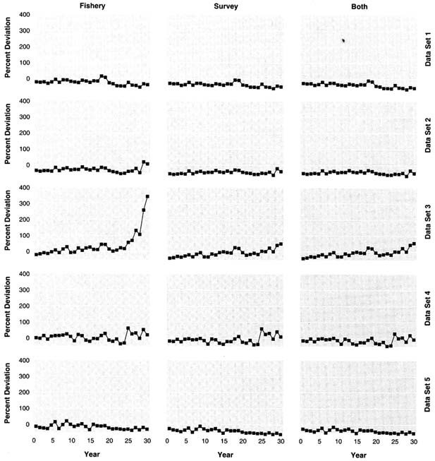
The true exploitable biomass and the fishery and survey indices of exploitable biomass over time are shown for each data set in Figure 5.2. Each series has been scaled by its mean to show relative patterns over time. Except for data set 3, the survey index has the same pattern as biomass; for data set 3, the doubling of catchability causes the survey index to underestimate relative biomass at the beginning and to overestimate relative biomass at the end of the period. For each data set, the fishery index does not have the same trend as exploitable biomass because of the increasing catchability of the fishery over time, the decreased age selectivity in some data sets, and the dependence of catchability on biomass. The survey index is more variable than the fishery index; the survey relative error was 30% versus 20% for the fishery.
The committee sought assistance from National Marine Fisheries Service (NMFS) analysts who regularly use the major types of stock assessment methods for real assessments. The models tested (listed in order of complexity) included a production model; two versions of a delay-difference model; and age-structured analyses using ADAPT, a spreadsheet, Stock Synthesis, and Autodifferentiation Model Builder (ADMB, a commercial
TABLE 5.1 Characteristics of Simulated Data Sets
|
Data Set |
Population Trend |
Age at 50% Selectivity |
Underreporting |
Survey Catchability |
|
1 |
Depletion |
Lower later |
None |
Constant |
|
2 |
Depletion |
Lower later |
30% |
Constant |
|
3 |
Depletion |
Lower later |
None |
Higher later |
|
4 |
Depletion |
Constant |
None |
Constant |
|
5 |
Recovery |
Constant |
None |
Constant |
package).* The spreadsheet implementation contained features similar to the Stock Synthesis program, but was a simpler implementation of the generic age-structured assessment (ASA) model. Further details about the implementation of these methods are given later in this chapter. The committee also utilized the services of a non-NMFS expert who performed additional ADAPT analyses. Data sets were sent to analysts in mid-March 1996 (see Appendix F for transmittal letter). Although the purpose of this exercise was to compare methods, the implementation of each method was affected by complex interactions among the individuals involved in the analyses, subjective and objective modeling decisions, the base model used, and the computer implementation of the model.
In addition to the five sets of catch, age composition, CPUE, and survey data from years 1 to 30, analysts were given growth and maturity parameters (see Appendix E), the ageing error probability matrix (Richards and Schnute, 1992), and information about the structure of the population and the data. Analysts were not provided with information about natural mortality, catchability, selectivity, the recruitment process, or the amount of underreporting (although they were warned that underreporting might have occurred). Analysts were requested to perform the analyses with three combinations of abundance indices:
- CPUE data only (coded "F")
- Survey data only ("S")
- Both CPUE and survey data ("B")
Analysts were asked to perform these analyses independently, that is, not to use results of one analysis to initiate others or to work with analysts using other methods.
As mentioned earlier, the survey index has a greater relative error associated with it than does the fishery index. In other aspects, the survey index is less variable because surveys either are intentionally designed to be unchanging over time (e.g., same gear, sampling design, sampling methods, and sampling areas) or are changed only with associated calibration experiments to ensure that survey data are comparable over time. Thus, catchability and selectivity for the survey data were assumed to be constant (except for catchability in data set 3). Randomized sampling designs used in surveys reduce the hyper stability effect. Conversely, commercial fishers learn and change gear, fishing areas, and fishing methods to maintain or increase their harvests. The data sets provided to analysts are representative of differences known to exist between survey and fisheries data. The committee deliberately constructed the simulation according to conventional wisdom that a survey should provide a better index of abundance than data from a fishery. Nevertheless, the committee could have just as easily interchanged the fishery and the survey to make the survey the bad source of information. Hence, the simulation should be interpreted as having contained two indices of abundance, one of which was usually a good measure of abundance, and the other not.
Analysts' results were received near the beginning of May 1996 and summarized prior to the committee's
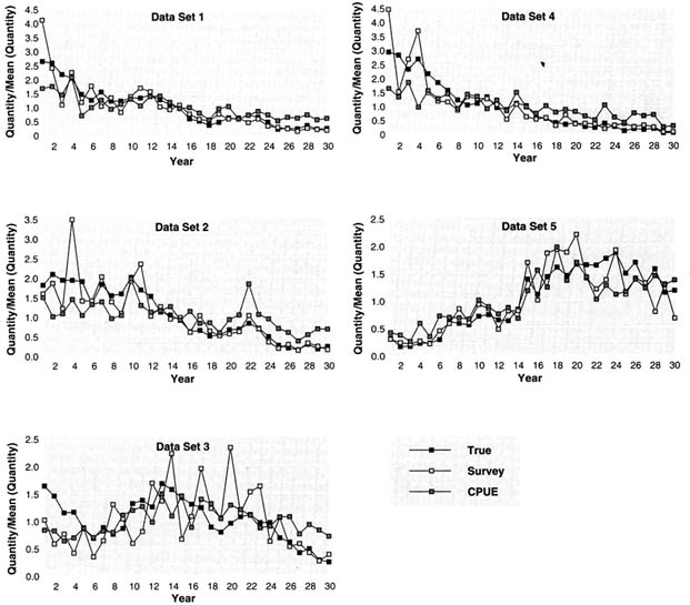
FIGURE 5.2 True exploitable biomass, survey biomass index, and fishery CPUE for the five simulated data sets. Data are plotted as quantity divided by the mean of the quantity over the 30 simulated years.
May meeting. Analysts cautioned the committee that the time they had available for the analyses was limited compared to a normal stock assessment. They noted that other information they would normally have available for doing a stock assessment (species characteristics, reports from harvesters and biologists, and other detailed information) was not given to them in this exercise. Such factors may have compromised the ability of analysts to obtain the absolutely best estimate, and the results presented herein do not necessarily reflect real-world conditions,* but all analysts operated under the same constraints, so this exercise constitutes a reasonable comparison of
methods. One other caveat is that each data set represented the results of one replication of a stochastic process. The possibility that any given data set was extreme cannot be eliminated. Other caveats from the analysts will be discussed more completely in a planned National Oceanic and Atmospheric Administration (NOAA) Technical Memo that presents the analysts' reports.
The committee met with analysts on May 14, 1996. Each analyst presented the model results, as well as an indication of problems or insights gained in the analysis. The true values of biomass, recruitment, and exploitation were compared with analysts' estimates. The committee and analysts discussed what further work should be undertaken.
Three types of additional analyses were performed after the May meeting. First, because analysts estimated and used different values of natural mortality in the initial set of model runs (ranging from 0.15 to 0.25), the committee requested that they repeat the analyses with a common value for natural mortality equal to the true average natural mortality of 0.225. The committee asked four analysts to perform these in-depth analyses for the (1) ADAPT, (2) ASA spreadsheet, (3) Stock Synthesis, and (4) ADMB age-structured models. For each of the simulated scenarios, analysts were asked to use the three combinations of fishery and survey data, as in the previous analyses.
Second, a standard set of definitions of key management variables was agreed to and it was decided to calculate TAC (total allowable catch) in year 31 using a rate based on F40% (as described in Chapter 4). Some analysts tried additional methods to improve the assessment; these results are reported later in this chapter.
Most existing assessment methods provide some estimate of precision of the parameter estimates. However, these are based on the structure of the assessment model being correct. Thus, unless the model structure is flexible enough to allow for major sources of uncertainty about the processes and data to be incorporated, estimates of precision tend to underestimate the true uncertainty in the assessment. It would have taken a considerable amount of additional work by both the analysts and the committee to evaluate estimates of uncertainty, so this was not done.
Finally, the committee decided to undertake retrospective analyses (see Chapter 3 for more detail about this subject) to determine the persistence of over- or underestimation of population parameters over time by the different methods. Although initial results indicated that the different methods were often able to recognize that the stock was severely depleted (or substantially recovered) at the end of the simulated time period, earlier recognition would be necessary for management to react in a timely fashion. Thus, retrospective analysis is important to determine how long it would take for the assessments to recognize underlying stock trends. The analysts were to use their methods on 16 subsets of the total data set: years 1-15, 1-16, …, 1-30.
The committee collected the results of these analyses in August 1996, summarized them, and conducted additional statistical analyses of the results to test whether trends of estimates and trends of the true values were parallel (even if biased). The committee met in August 1996 to review results obtained to that point, to formulate additional analyses of the simulation results, and to develop preliminary findings and recommendations.
Simulation Results
This section describes the approaches taken for each specific model and presents the simulation results. The simulation results using mortality rates selected by the analysts are contrasted with results using the true M (natural mortality rate). Methods are compared on the basis of summary statistics related to important management parameters. Finally, the committee's additional analyses of model performance and retrospective analyses are presented.
Results Using Estimated M
Production Models
The production model used is described in Prager (1994). The production model estimates productivity parameters from total harvest and indices of biomass (CPUE, survey abundance over ages). No age-structured
information was used. It was difficult for this model to produce reasonable estimates for many data set-data source combinations. In particular, no reasonable estimates could be obtained from data set 3, the most difficult one, because neither CPUE nor survey data were consistent indices of abundance over time.
Estimates by this method are shown in Table 5.2, along with the analyst's confidence in the results. Estimates were provided for MSY (maximum sustainable yield)*, FMSY, EMSY, BMSY, B30, and fishing mortality and biomass in year 30 relative to the MSY level (Frel and Brel, respectively).† The committee calculated relative fishing mortality from the fishing effort information and relative biomass from exploitable biomass values provided by the analyst.
The analyst's confidence in the results was generally low, with some moderate confidence in results from data set 4 (the easiest). When both fishery and survey data were used, estimates of MSY were 4 to 20% below the true value. However, estimates of absolute and relative fishing mortality and biomass generally were not close to the true values. Curiously, the use of fishery CPUE alone sometimes produced estimates close to the true values, even though the simulated CPUE was a biased measure of biomass. Nevertheless, the estimates often differed substantially from the true values, suggesting a lack of robustness of production models for data such as the simulated data used in this study.
The analyst cogently summarized the limitations of production models as follows: ''The simulated data sets do not seem well suited to simple production modeling, and confidence in the quantitative validity of most of the results obtained is low. Noisy data, poorly correlated CPUE and survey indices, and relatively constant effort levels all probably contribute to this situation. Without knowing the underlying population model and conducting simulations, it is impossible to say to what degree age-structure effects also contribute. The apparently high fishing mortality rates and the extensive age-structured data available suggest that these fisheries are better suited to analysis by cohort-based methods. This suggestion is strengthened by several sets of simulated data in which apparently constant fishing effort leads to a population increase and then a decrease—such a scenario is incompatible with the assumptions underlying simple production models. This suggests either environmental forcing of recruitment, nonconstant catchability, or both."
Delay-Difference Models
Two analysts fitted the Schnute version of Deriso's delay-difference model (Deriso, 1980; Schnute, 1985), using total harvest data, the two indices of abundance, and a recruitment index (age 5 fishery or survey data for the first delay-difference method [DD] and age 3 [data sets 1-4] or age 4 [data set 5] fishery or survey data for the second delay difference method [DDKF]). For both models, recruitment was assumed to be knife-edge (i.e., all fish are vulnerable to the fishery at the same age). The population parameters estimated from this model therefore may not be strictly comparable to the true parameters, which were calculated from the age-dependent selectivity function.
The DD method was a measurement error model. Results from this model included estimates of biomass, recruitment, and fishing mortality. Natural mortality values were the same as those used in the first Stock Synthesis method described below (0.251. 0.251, 0.169, 0.201, and 0.191 for data sets 1 to 5, respectively).
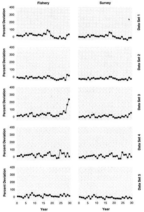
For many of the DD results (Figure 5.3), deviations in exploitable biomass from the true value showed little trend, but there are substantial deviations in absolute values over the entire time period. Not surprisingly, the use of only fishery data (left panel of Figure 5.3) produced the most extreme deviations because the fishery data had a time trend in catchability that was not incorporated in the delay-difference models. Use of fishery data tended to lead to overestimates of biomass and failure to estimate the correct trend in exploitation fraction. Better results were obtained by using survey data alone or by using both data sources, but substantial discrepancies still remained. The deviations for data set 4 were particularly surprising, because this data set was relatively well
TABLE 5.2 Comparison of Results of Single Runs of Production Models with True Valuesa
|
Data Set |
1 |
1 |
1 |
True |
2 |
2 |
True |
3 |
True |
|||
|
Index |
Fb |
S |
B1 |
|
F |
B1 |
|
All |
|
|||
|
MSY |
580 |
90 |
300 |
312 |
995 |
218 |
240 |
|
315 |
|||
|
Frel |
1.6 |
13 |
2.2 |
1.4 |
1.9 |
2.7 |
1.8 |
|
2.0 |
|||
|
Brel |
0.18 |
0.11 |
0.23 |
0.14 |
0.07 |
0.21 |
0.19 |
|
0.36 |
|||
|
Confidence |
Lc |
L |
L to N |
|
L to N |
L |
|
N |
|
|||
|
FMSY |
0.21 |
0.03 |
0.31 |
0.196 |
0.21 |
0.25 |
0.158 |
|
0.151 |
|||
|
EMSY |
983 |
nad |
1236 |
1223 |
917 |
1169 |
949 |
|
1096 |
|||
|
BMSY |
2744 |
3183 |
954 |
1924 |
4639 |
1162 |
1820 |
|
2480 |
|||
|
E30 |
|
1703 |
|
1694 |
|
2139 |
||||||
|
B30 |
480 |
430 |
236 |
276 |
324 |
322 |
346 |
|
903 |
|||
|
Data Set |
4 |
4 |
4 |
4 |
True |
5 |
True |
|
||||
|
Index |
F |
S |
B1 |
B2 |
|
F |
|
|||||
|
MSY |
2470 |
300 |
430 |
480 |
513 |
635 |
564 |
|
||||
|
Frel |
1.6 |
3.4 |
1.7 |
1.5 |
1.4 |
0.51 |
0.6 |
|
||||
|
Brel |
0.03 |
0.11 |
0.17 |
0.18 |
0.05 |
1.4 |
2.09 |
|
||||
|
Confidence |
VL |
L to M |
L to M |
L to M |
|
L |
|
|||||
|
FMSY |
0.20 |
0.12 |
0.28 |
0.28 |
0.252 |
0.13 |
0.28 |
|
||||
|
EMSY |
128 |
na |
180 |
169 |
1827 |
2123 |
2025 |
|
||||
|
BMSY |
12600 |
2540 |
1546 |
1701 |
2477 |
4738 |
2473 |
|
||||
|
E30 |
|
2552 |
|
1139 |
|
|||||||
|
B30 |
388 |
309 |
264 |
290 |
115 |
6950 |
5158 |
|
||||
|
a The analyst examined all data sets and sources of data; those not given in this table were assigned no confidence by the analyst and productivity results were not meaningful. The analyst would not normally report absolute estimates FMSY and BMSY, believing that relative values are more accurate and more useful for management. They are included in this table for scientific interest. The major characteristics of the five data sets are given in Table 5.1 True values are those calculated by the committee from known parameter values. bData source: F = fishery; S = survey; B1 = both, using standard methods; B2 = both, using alternative techniques such as iterative reweighting or a combined survey-fishery index. cConfidence: M = moderate, L = low, VL = very low, N = none dEstimates of EMS are not available from production models using survey indices only. However, the estimate of Frel (identical to Erel) serves the same purpose and is often more useful in practice. NOTE: FMSY, EMSY, and BMSY are fishing mortality, effort, and biomass, respectively, at MSY. E30 and B30 are effort and biomass in year 30. Frel and Brel are fishing mortality and biomass in year 30 relative to FMSY and BMSY. E30 is a known value used to calculate Frel. |
||||||||||||
structured. Nevertheless, the delay-difference model, by utilizing some information about age structure, showed improved estimates compared with production models. However, poor indices of abundance and the failure to use more age-structured data led to estimates that were more variable than the age-structured models discussed below. Models were rerun after the true average M value was provided, and those results are discussed in the following section.
ADAPT
The ADAPT approach is described in Gavaris (1988), Conser and Powers (1989), Restrepo and Powers (1991), and Conser (1993). It is essentially a cohort analysis on catch-age data where indices of abundance are included to estimate a relatively small number of parameters. The major assumption is that there are no errors in the catch-age data.

The team of analysts who met for two days to perform the ADAPT analyses found that the ageing error matrix provided by the committee was more suitable to forward types of analyses such as ASA, SS, and ADMB and decided that they could not use such information. An M value of 0.15 was used in the ADAPT analyses, based on heuristic examination of the data and an attempt to estimate M from the data after making some assumptions about selectivity and catch variability.
Generally, the procedure used was (1) to examine the data and pool it beyond some age into a plus group, (2) to obtain selectivity estimates using a separable virtual population analysis, (3) to fix the ratio of fishing mortality for the plus group to the next-youngest age, and (4) to run a nonlinear least-squares procedure to estimate population parameters. Estimates of total and exploitable biomass, recruitment, spawning stock biomass, total biomass averaged over the year (Bave), and average exploitation fraction (Y/Bave, where Y = yield) were calculated. Age-specific estimates of catchability were examined and trends were discovered in some data sets. Therefore, except for data set 5, fishery CPUE data were not used, despite the committee's request for these sets of analyses, because the ADAPT team did not believe the information was useful. For data set 5, this group attempted a fit of the combined survey and fishery CPUE.
The relative trend in the estimates obtained was similar to the other age-structured methods (Figure 5.4). However, estimates of abundance were negatively biased, because the choice of natural mortality of 0.15 was too low compared to the true average M of 0.225. These results confirm the general conclusion that underestimating natural mortality leads to underestimation of abundance. A consequence of underestimating abundance is a tendency to overestimate exploitation rate. The team did not compute TAC because the procedure it would have used would have taken more time than was available.
Separable ASA Models
A family of age-structured assessment models is based on a statistical formulation of age-structured information and the assumption that fishing mortality is separable into age-selectivity multiplied by a full-recruitment fishing mortality (Doubleday, 1976; Fournier and Archibald, 1982; Deriso et al., 1985; Methot, 1989, 1990). A generic age-structured assessment model with these characteristics was formulated in a spreadsheet (ASA). It included a modification of the method assuming that all catch was taken halfway through the year and demonstrated that this approximation was accurate. The likelihood function consisted of a multinomial component that incorporated ageing error and a residual sum of squares term for the logarithm of each abundance index (number per boat-day from the fishery or survey catch in numbers, either pooled or by age). For data set 3, ASA assumed different catchabilities for years 1-15 and years 16-30 due to the change in survey vessel. An asymptotic curve for survey selectivity was used, but the analyst who ran ASA noted that he would have considered using a dome-shaped selectivity curve (the true situation) if he had other information to justify that choice. This spreadsheet model had similar characteristics to the Stock Synthesis model described next, but was simpler.
Estimates of natural mortality came from the Alverson-Carney procedure (based on longevity of a species and growth) and were 0.251, 0.251, 0.169, 0.201, and 0.191, for data sets 1 to 5, respectively. Trends from the survey and the fishery did not match, and the analyst suspected that the fishery data had trends in catchability. This analyst did a great deal of preliminary data exploration work to help him discover structural features in the data sets that improved his analyses. Deviations of estimated exploitable biomass from the true value were generally smaller when using only survey data or both compared to only fishery data (Figure 5.5). The ASA method usually resulted in less trend in the deviations over time than the methods previously described.
The Stock Synthesis method was implemented in a computer program as described in Methot (1989, 1990) and denoted SS-P in this report. A natural mortality value of 0.2 was used. Some models with constant recruitment were fitted to the data to mimic a production model. No results were presented from these analyses because recruitment was obviously not constant. The basic configuration of the model accounted for ageing error, used logistic curves for fleet and survey selectivity, and calculated fishing mortality values that equated the observed and predicted catch biomass values each year. The analyst calculated effective sample sizes from the mean squared error and showed that these were similar to actual sample sizes, which suggested that the SS-P


models were not overparameterized. The program used was able to project population sizes into the future under a fishing mortality policy and could readily produce retrospective analyses.
AD Model Builder
This method was based on the work of Fournier and Archibald (1982) as incorporated into a computer software product called Autodifferentiation Model Builder. Analyses using ADMB were conducted by a team composed of one NMFS scientist and a colleague from outside NMFS. ADMB is similar in character to Stock Synthesis, with some additional model features. ADMB has the capability of adding process errors in the recruitment, selectivity, catchability, and natural mortality parameters. A Bayesian framework allows results to be synthesized in terms of posterior probability distributions for selected population parameters. Because the program code is compact, it was easy to carry out retrospective analyses. Of all the models, this method was the most complex, with some models having in excess of 400 parameters. Similar to other methods, a logistic curve was used for fishery and survey selectivities in the ADMB model.
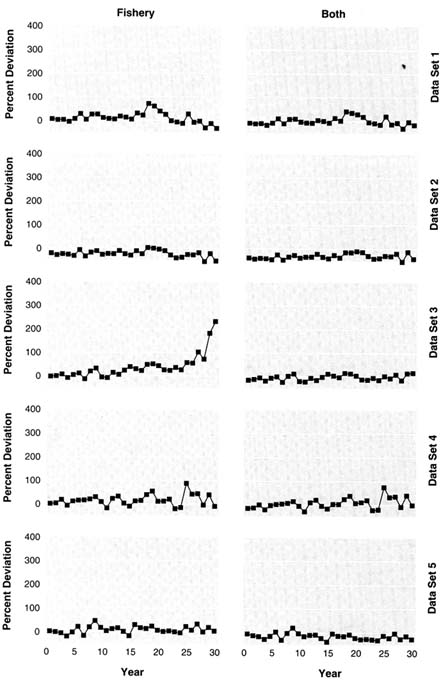
The base model (ADMB1) assumed that fishing mortality at age and year was the product of age-specific fishery selectivity, catchability, fishing effort, and a process error term. Recruitment was assumed to be random about a mean value. The objective function was the sum of a modified x2 goodness-of-fit function of the age composition data, lognormal error terms for fishing effort and recruitment, and a lognormal prior distribution for M with a mean of 0.2 and a standard deviation of 0.15. In model ADMB2, additional parameters were added to the fishery selectivity function to account for changes in selectivity over time. As with previous models, results were better when survey data were used alone than when both data sets or fishery data alone were used (Figures 5.9 and 5.10). In model ADMB3, applied only to data set 1, additional parameters were added for natural mortality deviations over time.
Comparison of Exploitable and Total Biomass* by Data Set
Graphs of exploitable and total biomass for all age-structured methods conducted with estimated M values are shown in Appendix I for the five data sets. For data set 1 (Figures I.1 and I.6), most estimated series show the correct overall pattern of decline over time. The estimates of exploitable biomass are generally greater than the true biomass for the first part of the series, but most converge toward the true biomass near the end of the series. Notable exceptions are the models that use only the biased fishery data as an abundance index. It should be noted that overestimation observed in the early part of the series did not occur with total biomass (Figure I.6).
For data set 2 (Figures I.2 and I.7), the pattern of decline was captured by models that used survey data. There was a tendency for the models to underestimate exploitable biomass. This difference from data set 1 can be attributed to the underreporting of catch that was included in data set 2.
For data set 3 (the "difficult" data set, Figures I.3 and I.8), models using only fishery data or those that did not use separate parameters for the two survey vessels tended to grossly overestimate exploitable and total biomass. Other deviations could have been caused by the incorrect specification of natural mortality and changes in age selectivity over time. All models overestimated biomass at the end of the series, sometimes dramatically. No model estimated exploitable biomass particularly well for this data set, although several models captured the overall trend.
For data set 4 (the "easy" data set, Figures I.4 and I.9), most models estimated the correct trend in biomass, showing that the population was depleted at the end of the series. As in other data sets, models using only fishery data tended to overestimate biomass, particularly at the beginning of the series.
For data set 5 (Figures I.5 and I.10), the only one with an increasing trend in biomass, all models showed an increase in exploitable and total biomass over time. However, there was a general tendency to underestimate the amount of recovery in the population. Unlike the other data sets, estimates were more accurate in an absolute sense at the beginning of the series than at the end.


Results Using True Average M
The delay-difference method DDKF and the four age-structured modeling methods were rerun using a true average M of 0.225. The following sections describe the results of the second set of model runs and discuss the effects of M value on stock assessment results.
Delay-Difference
The DDKF method included Kalman filtering and both measurement and process error. Results from DDKF included estimates of biomass and recruitment; true exploitation fraction was determined by dividing yield by biomass. Biomass and recruitment estimates were calculated using F and S data. For the process error model, the analyst conducted a separate investigation of the estimability of M. Results from DDKF were qualitatively similar to results from DD (Figure 5.11). One notable feature of the DDKF model was its ability to estimate accurately the amount of process error present in some data sources. This result suggests that stock assessment methods incorporating both measurement and process error reflect the uncertainty in both the data and the population more accurately.
ADAPT
The ADAPT method was rerun by an individual not associated with the group that performed the initial ADAPT analysis. The National Research Council's (NRC's) ADAPT method assumed (as was true) that a Gamma function describes the true shape of the gear selectivity of the simulated survey data sets and that a logistic selectivity curve describes the true shape of the gear selectivity of the simulated fishery data sets for the terminal year.
Separable ASA Models
Knowing the correct true average M, the analyst who ran the ASA model attempted to estimate natural mortality from data set 1 using only the survey index. The likelihood profile was centered about 0.28, which was further from the true value than was the original value used, suggesting that the available data did not provide useful information for estimating natural mortality. One possible explanation for this result is that the use of an asymptotic survey selectivity curve, when survey selectivity was actually dome shaped, resulted in confounding natural mortality with survey selectivity parameters (Thompson, 1994). For exploitable biomass in year 1, estimates were more accurate using the true average M for the first four data sets, but not for the fifth. For exploitable biomass in year 30, estimates were closer for data sets 1, 2, and 4, but not for 3 and 5. For TAC in year 31, estimates were closer to the truth for data sets 1, 2, and 5, but not for 3 and 4. Overall, estimates were more accurate using the true average M in 10 of the 15 cases, which is not significantly different from a 50:50 ratio (x2 test, p = .59).
Results from the SS-P3(S), SS-P7(F), and SS-P7(B) models with the true average M are shown in Table 5.3. For exploitable biomass, F40%, and TAC in year 31, overall estimates were more accurate using the true average M in 28 cases, less accurate in 15 cases, and the same in 2 cases; thus, the true M yielded significantly more accurate values for these three parameters (x2 test, p { .05).
ADMB
A final ADMB model (ADMB4) was constructed, using the true average M and incorporating time-series variations in fishery selectivity, fishery catchability, and natural mortality. For data set 3, the analyst chose not to incorporate two selectivity curves for the survey but rather allowed for time-specific deviations in catchability in the model and examined whether a trend in survey catchability occurred. Results are shown in Figure 5.12.

TABLE 5.3 Comparison of Some SS-P Results Using Original M (0.2) Versus True Average M (0.225)
Comparison of Methods Using Summary Statistics
The statistics provided by stock assessments that are most useful for management include recent estimates of biomass, the amount of historical decline, recommended catch limits (TACs), recommended exploitation fractions, and spawner and recruitment information such as average spawning biomass and average recruitment. Specifically, the following information was summarized:
- Exploitable biomass in year 30 (EB30)
- Ratio of BE in year 30 to EB in year 1 (EB30/EB1), a measure of population decline or building
- Total allowable catch in year 31 from an F40% exploitation strategy (TAC31)
- Ratio of TAC31 to projected exploitable biomass in year 31 (TAC31/
 31), the projected exploitation rate. Projected exploitable biomass in year 31 was obtained by multiplying each analyst's estimate of exploitable biomass in year 30 by the true ratio of EBs in years 31 and 30. This was done to determine the recommended exploitation fraction (TAC31/31) in a consistent manner for all models, because some analysts did not provide estimates of EB in year 31.
 - Average recruitment (
 ) from years 1 to 30
 - Average spawning biomass (
 )
)
Results for these management parameters are expressed in terms of relative error [(estimated - true)/true] for the various models, and results are shown separately for runs made with estimated versus the true M value in tables that follow. For the purpose of evaluating different models a modest goal for stock assessment is to obtain estimates of key management parameters within ±25% of the true values.
Results Averaged Across Data Sets
A summary of the results across data sets is presented to show the general performance of the models. The summary statistic used was the average of the absolute values of relative errors among the five data sets. The average of absolute relative errors is used to illustrate the precision of estimates compared to true values and the average of relative errors are used to illustrate the accuracy or bias. The absolute value indicates models that deviated in either direction from the truth (Table 5.4); results from individual data sets are presented in Tables 5.5 to 5.9 and can be used to examine the direction of the errors for the individual sets. Models that did not have results for all five data sets were excluded.
Results given in Table 5.4 show that there can be great deviations in management statistics from the true values. Figure 5.13 shows the results for exploitable biomass in year 30, with relative absolute deviations often exceeding 50%, comparing estimated M versus the true average M. Model runs that used only fishery data generally yielded the worst results, those that used only survey data were generally the best, and those that used both sources ranged from best to intermediate in their results. The success of runs with both data sources depended greatly on which model was used. Model runs with more complex treatment of fishery data (SS-P6, SS-P7, ADMB4) tended to have lower errors than those with simpler treatment (DD, ASA, SS-P3, NRC ADAPT), and a similar result was obtained when fishery data were used alone. Results obtained with the true average M were not much different from those with estimated M values, probably because the true average M used in the revised analyses was, in many cases, not that much different from the M used initially. The fact that the true population had varying M over time whereas analysts used constant M (except ADMB4) may have been more important than changes in average M.
Results for the ratio of biomass in year 30 to that in year 1 were similar to those for EB30 (compare Table 5.4B). This result was somewhat surprising because the committee expected it would be easier to estimate the overall change in populations than their absolute biomes levels.
The committee thought it was very important to consider the relative error in TAC, because this statistic is frequently the end point of assessment, being the recommended catch level to be taken in the next year.* The
TABLE 5.4A Average Absolute Values of Relative Errors [¦(estimated – true)/true¦] for Important Management Parametersa—Results with Estimated M
TABLE 5.4B Average Absolute Values of Relative Errors [¦(estimated – true)/true¦] for Important Management Parametersa—Results with M = 0.225
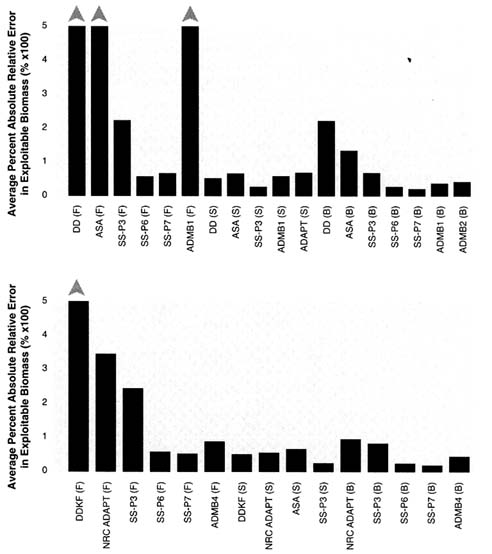
FIGURE 5.13 Average absolute values of relative errors for exploitable biomass in year 30. (Results prior to [upper panel] and after [lower panel] knowing the true M.)
relative error in TAC was comparable to the relative error in exploitable biomass, sometimes higher and sometimes lower (see Table 5.4). In many cases, it deviated more than 50% from the true value. As before, models using only survey data or both data sources fared better than those using only fishery data. The ratio of TAC to exploitable biomass (TAC31/![]() 31) is the recommended exploitation rate. The amount of relative error in this statistic was lower overall than for the previous statistics, especially for model runs using only fishery data (Table 5.4). Many model runs yielded relative errors well below 50%. For this statistic, the model used seemed also to be a factor: the NCR ADAPT and ADMB4 models had greater errors than other models, regardless of which combination of data was used. Average recruitment (
31) is the recommended exploitation rate. The amount of relative error in this statistic was lower overall than for the previous statistics, especially for model runs using only fishery data (Table 5.4). Many model runs yielded relative errors well below 50%. For this statistic, the model used seemed also to be a factor: the NCR ADAPT and ADMB4 models had greater errors than other models, regardless of which combination of data was used. Average recruitment (![]() ) and average spawning biomass (
) and average spawning biomass (![]() ) were estimated with less error overall than other management parameters. This is not surprising because these statistics are calculated over the entire time period, which averages out the positive and negative errors found in individual years.
) were estimated with less error overall than other management parameters. This is not surprising because these statistics are calculated over the entire time period, which averages out the positive and negative errors found in individual years.
Results by Data Set
Using Estimated M
Tables 5.5 to 5.9 present the relative errors in management variables for data sets 1 to 5, respectively. These tables show that average recruitment (![]() ) and average spawning biomass (
) and average spawning biomass (![]() ) are estimated with less error overall than other management parameters. The ADAPT model generally underestimated these because the natural mortality used was too low. Models using only fishery data (F) often overestimated average biomass, unless the models contained sufficient additional parameters to overcome the catchability patterns. For data set 2, many models underestimated
) are estimated with less error overall than other management parameters. The ADAPT model generally underestimated these because the natural mortality used was too low. Models using only fishery data (F) often overestimated average biomass, unless the models contained sufficient additional parameters to overcome the catchability patterns. For data set 2, many models underestimated ![]() and
and ![]() because of underreporting. The same thing occurred with data set 5 because biomass and recruitment were underestimated for the recovering population. For the first four management parameters related to exploitable biomass and TAC, the amount of error is quite variable among parameters and among models. The worst results are generally obtained by using only fishery data for all data sets. However, the tendency for most models using survey data to underestimate biomass in data set 5 results in the fishery-only models sometimes producing estimates that are closer to the truth for this data set. The underestimation could have been due to the particular set of random numbers used for this data set, so it would not be appropriate to conclude that assessments based on commercial CPUE generally would be better.
because of underreporting. The same thing occurred with data set 5 because biomass and recruitment were underestimated for the recovering population. For the first four management parameters related to exploitable biomass and TAC, the amount of error is quite variable among parameters and among models. The worst results are generally obtained by using only fishery data for all data sets. However, the tendency for most models using survey data to underestimate biomass in data set 5 results in the fishery-only models sometimes producing estimates that are closer to the truth for this data set. The underestimation could have been due to the particular set of random numbers used for this data set, so it would not be appropriate to conclude that assessments based on commercial CPUE generally would be better.
For data set 1, examination of Table 5.5A shows that the goal of being within 25% of the true value was achieved for at least two of the first four management parameters (related to exploitable biomass and TAC for the DD(S), SS-P3(B), SS-P3(S), SS-P6(B), and SS-P7(B) models [notation indicates model followed by data set in parentheses]). In only one case (SS-P7[B]) however, was this goal obtained for all four management parameters. For data set 2, the 25% criterion was achieved for at least two parameters with the DD(S), SS-P3(S), SS-P6(B), SS-P6(F), and SS-P7(B) models, but no model met the criterion for all four parameters (Table 5.6A). For data set 3, the ''hard" data set, the criterion was achieved for two parameters only for the DD(S) and SS-P7A(B) models, and neither of these models achieved the criterion for all four parameters (Table 5.7A). For data set 4, the so-called easy data set, the criterion was achieved for the DD(S), AD(F), AD(B), SS-P3(S), SS-P3(F), SS-P3(B), SS-P6(F), SS-P6(B), SS-P7(F), and SS-P7(B) models, but only SS-P3(S) achieved the criterion for all four parameters (Table 5.8A). For data set 5, the criterion was achieved for at least two parameters by the DD(F), DD(S), ASA(S), SS-P6(F), SS-P6(B), SS-P7(F), and SS-P7(B) models (Table 5.9A). The criterion was met for all four management parameters only for the ASA(S) and the SS-P7(F) models. The DD(S) model met the criterion for at least two parameters for all five data sets. Otherwise, no single model performed superlatively across all data sets and all management parameters.
Using True Average M
Results using the true average M value are presented in Tables 5.5B to 5.9B. By using the true average M value, ![]() and
and ![]() are estimated with even less error overall than results obtained without knowledge of the true average M. This probably results from a combination of use of the true average M and use of more complicated models in the second round of model runs that corrected some biases in the earlier models. However, in some cases, using the correct M in a model did not result in an improvement. For example, for data set 3, the second-run models tended to overestimate average recruitment, which did not occur with the first run. Whether this was due to the variability in M, confounding of model parameters, or random chance is unknown.
are estimated with even less error overall than results obtained without knowledge of the true average M. This probably results from a combination of use of the true average M and use of more complicated models in the second round of model runs that corrected some biases in the earlier models. However, in some cases, using the correct M in a model did not result in an improvement. For example, for data set 3, the second-run models tended to overestimate average recruitment, which did not occur with the first run. Whether this was due to the variability in M, confounding of model parameters, or random chance is unknown.
For data set 1, relative errors were less than 25% for at least two of the exploitable biomass and TAC statistics for the NRC ADAPT(S), SS-P3(S), SS-P3(B), SS-P6(B), SS-P6(F), and SS-P7(B) models; only the latter model met this criterion for all four parameters (Table 5.5B). For data set 2, at least two statistics achieved the criterion for the ADMB4(B), NRC ADAPT(S), SS-P3(S), SS-P3(B), SS-P6(F), SS-P6(B), and SS-P7(B) models. No model achieved the criterion for all four parameters, because the underreporting led to underestimation of biomass with resultant effects on TAC (Table 5.6B). For data set 3, the 25% criterion was achieved for two statistics only by the DDKF(S) model (Table 5.7B). As with the prior results, there was a general tendency to overestimate biomass and TAC statistics for this data set, often by a wide margin. For data set 4, all models (except DDKF and
TABLE 5.5A Data Set 1: Summary of Relative Error [(estimated—true)/true] in Parameters Important for Management—Results with Estimated M
TABLE 5.5B Data Set 1: Summary of Relative Error [(estimated—true)/true] in Parameters Important for Management—Results with Estimated M
TABLE 5.6A Data Set 2: Summary of Relative Error [(estimated – true)/true] in Important Management Parameters—Results With Estimated M Values
TABLE 5.6B Data Set 2: Summary of Relative Error [(estimated – true)/true] in Important Management Parameters—Results with M = 0.225
TABLE 5.7A Data Set 3: Summary of Relative Error [(estimated – true)/true] in Important Management Parameters—Results With Estimated M
NRC ADAPT) had at least two statistics within 25% of the truth. All four statistics met the criterion for the ADMB4(B), SS-P3(S), SS-P3(B), SS-P6(B), and the SS-P7(B) models (Table 5.8B). For data set 5, all models achieved the criterion for at least two statistics, except for the ADMB4(B), NRC ADAPT, SS-P3(B), and SS-P3(F) models (Table 5.9B); SS-P6(F), SS-P6(B), SS-P7(B), and SS-P7(F) fell within 25% for all four statistics.
Overall, Tables 5.5B-5.9B show that errors in exploitable biomass and TAC are less than 25% (bold entries) more frequently for complex models (defined here as ADMB4, SS-P6, and SS-P7) than for simple models (defined here as DDKF, NRC ADAPT, ASA, and SS-P3); bold entries for estimates of exploitable biomass occur for 23% (44%) of simple (complex) model runs; bold entries for estimates of TAC occur for 17% (35%) of simple (complex) model runs. Table 5.10 suggests some modest improvement in management parameters by having the true average M; for example, the percent success (as defined in Table 5.10) was greater for two to four of the five data sets (depending on the variable) when M was set to its true mean. Yet, it should be noted that no one model performed superbly in all cases and for all management parameters.
Effect of M Value
The results from these comparisons suggest that having the correct value of M did not significantly improve the assessment results for the ASA and SS models used before and after the true average M value was revealed. This conclusion appears to be independent of which summary statistic or which data sources are used in the assessment. The reason for this modest effect of incorrect M on all models is probably that variability in M, ageing
TABLE 5.7B Data Set 3: Summary of Relative Error [(estimated – true)/true] in Important Management Parameters—Results with M = 0.225
|
Model |
Data source |
EB30 |
EB30 EB1 |
TAC31 |
TAC31
|
|
|
|
DDKF |
F |
11.50 |
5.49 |
16.01 |
0.36 |
-0.06 |
na |
|
DDKF |
S |
-0.03 |
0.52 |
-0.13 |
-0.10 |
-0.60 |
na |
|
ADMB4 |
F |
3.44 |
4.75 |
9.11 |
1.28 |
0.53 |
0.18 |
|
ADMB4 |
B |
0.54 |
1.68 |
1.97 |
0.93 |
0.12 |
-0.10 |
|
NRC ADAPT |
F |
2.64 |
6.50 |
13.62 |
3.01 |
0.81 |
2.02 |
|
NRC ADAPT |
S |
1.25 |
1.22 |
2.75 |
0.67 |
0.23 |
1.22 |
|
NRC ADAPT |
B |
1.53 |
1.48 |
3.28 |
0.69 |
0.26 |
1.27 |
|
ASA |
S |
1.05 |
0.73 |
1.88 |
0.40 |
0.16 |
0.22 |
|
SS-P3 |
B |
2.98 |
2.81 |
4.89 |
0.48 |
0.46 |
0.12 |
|
SS-P3 |
F |
5.07 |
3.52 |
7.99 |
0.48 |
0.69 |
0.46 |
|
SS-P3 |
S |
1.06 |
0.95 |
1.84 |
0.38 |
0.17 |
0.02 |
|
SS-P6 |
B |
1.24 |
1.14 |
2.13 |
0.40 |
0.20 |
0.02 |
|
SS-P6 |
F |
2.32 |
1.43 |
3.68 |
0.41 |
0.39 |
0.32 |
|
SS-P7 |
B |
1.03 |
1.11 |
1.48 |
0.22 |
0.13 |
-0.02 |
|
SS-P7 |
F |
1.63 |
1.26 |
2.12 |
0.19 |
0.24 |
0.21 |
|
SS-P3Aa |
B |
3.58 |
3.18 |
5.95 |
0.52 |
0.55 |
0.15 |
|
SS-P3A |
F |
5.19 |
3.61 |
8.17 |
0.48 |
0.71 |
0.46 |
|
SS-P3A |
S |
0.62 |
0.45 |
1.15 |
0.33 |
0.10 |
0.02 |
|
SS-P6A |
B |
0.59 |
0.43 |
1.11 |
0.32 |
0.10 |
0.01 |
|
SS-P6A |
F |
2.19 |
1.34 |
3.49 |
0.41 |
0.38 |
0.31 |
|
SS-P7A |
B |
0.28 |
0.27 |
0.41 |
0.10 |
0.03 |
-0.04 |
|
SS-P7A |
F |
1.54 |
1.18 |
2.00 |
0.18 |
0.22 |
0.20 |
|
TRUE |
|
903 |
0.156 |
70 |
0.094 |
853 |
1,322 |
|
NOTE: For the first four management statistics, values within 25% of the truth are shown in boldface type. a Two catchability parameters were used, corresponding to the change of survey vessel. |
|||||||
error, changes in catchability and selectivity, and random variability dominated assessment results more so than the choice of a specific M value. The other reason is that many analyses used an estimated M value not too far from the true average M. One notable exception was the application of the ADAPT model to these simulated data sets. Dramatic underestimation of biomass occurred using an M of 0.15. When the correct average M was used, the NRC ADAPT results were better than the original ADAPT results but still showed major departures from the true values. Therefore, other factors still dominated the assessment results.
The committee expected that relative measures of biomass and exploitation would be estimated more accurately than absolute quantities. Examination of Tables 5.5 to 5.9 shows that this expectation was not fulfilled often. The estimated decline or increase in population over the time period (EB30/EB1) often had as much or more error than the most recent estimate of exploitable biomass (EB30). Similarly, the projected exploitation fraction in year 31 (TAC31/![]() 31) frequently had greater error than the projected catch limit (TAC31) itself. When this occurred, the reason was often that exploitable biomass was underestimated but TAC was overestimated, which resulted in even greater error in the exploitation fraction.
31) frequently had greater error than the projected catch limit (TAC31) itself. When this occurred, the reason was often that exploitable biomass was underestimated but TAC was overestimated, which resulted in even greater error in the exploitation fraction.
Additional Analyses
Ability of Models to Detect Abundance Trends
Visual comparison of biomass trends from the assessment models in Appendix I (Figures I.1 to I.10) shows that in many cases the lines (1) do not coincide with the true values and (2) are not parallel with true values. For example, the trends in exploitable and total biomass estimated by ADMB1(F) for data set 2 (Figures I.2 and I.7)
TABLE 5.8A Data Set 4: Summary of Relative Error [(estimated—true)/true] in Important Management Parameters—Results with Estimated M
TABLE 5.8B Data Set 4: Summary of Relative Error [(estimated – true)/true] in Important Management Parameters—Results With M = 0.225
TABLE 5.9A Data Set 5: Summary of Relative Error [(estimated – true)/true] in Important Management Parameters—Results with Estimated M
TABLE 5.9B Data Set 5: Summary of Relative Error [(estimated – true)/true] in Important Management Parameters—Results with M = 0.225
TABLE 5.10 Number of Times That 25% Criterion Was Achieved
|
Results with Estimated M |
|
Results with M = 0.225 |
|
|||||
|
Data |
EB30 |
EB30 EB1 |
TAC31 |
TAC31
|
EB30 |
EB30 EB1 |
TAC31 |
TAC31
|
|
1-F |
0 |
2 |
0 |
0 |
1 |
2 |
0 |
0 |
|
1-S |
2 |
1 |
3 |
2 |
3 |
2 |
1 |
1 |
|
1-B |
4 |
3 |
2 |
2 |
3 |
3 |
2 |
2 |
|
% Success |
27% (22)a |
32% (19) |
33% (15) |
27% (15) |
47% (15) |
47% (15) |
20% (15) |
20% (15) |
|
2-F |
2 |
1 |
0 |
1 |
2 |
1 |
0 |
0 |
|
2-S |
1 |
3 |
1 |
1 |
1 |
2 |
2 |
1 |
|
2-B |
2 |
4 |
1 |
1 |
1 |
5 |
2 |
1 |
|
% Success |
25% (20) |
44% (18) |
14% (14) |
21% (14) |
27% (15) |
53% (15) |
27% (15) |
13% (15) |
|
3-F |
0 |
0 |
0 |
3 |
0 |
0 |
0 |
2 |
|
3-S |
1 |
0 |
1 |
1 |
1 |
0 |
0 |
1 |
|
3-B |
1 |
0 |
1 |
2 |
0 |
0 |
0 |
2 |
|
% Success |
8% (25) |
0% (25) |
11% (19) |
32% (19) |
7% (15) |
0% (15) |
0% (15) |
33% (15) |
|
4-F |
3 |
3 |
1 |
2 |
3 |
4 |
0 |
2 |
|
4-S |
1 |
2 |
1 |
3 |
1 |
2 |
1 |
1 |
|
4-B |
4 |
4 |
1 |
2 |
4 |
4 |
4 |
5 |
|
% Success |
36% (22) |
50% (18) |
19% (16) |
44% (16) |
53% (15) |
67% (15) |
33% (15) |
53% (15) |
|
5-F |
2 |
3 |
2 |
5 |
2 |
5 |
4 |
4 |
|
5-S |
2 |
2 |
1 |
2 |
2 |
3 |
1 |
3 |
|
5-B |
0 |
5 |
0 |
4 |
2 |
2 |
2 |
3 |
|
% Success |
20% (20) |
53% (19) |
23% (13) |
85% (13) |
40% (15) |
67% (15) |
47% (15) |
67% (15) |
|
a Numbers in parentheses indicate number of values included in percentage calculations (determined from parameter values given in Tables 5.5-5.9, excluding cells for which "na" is noted). |
||||||||
predict a much larger biomass than actual and a very different trajectory over time. Noncoincident but parallel trends of the estimated quantities may be acceptable for stock assessment purposes because the estimated trend is unbiased despite the error in estimation of absolute abundance. That is, even if actual stock abundance values are unknown, it is useful to be able to detect relative increases and decreases of stock abundance over time. Nonparallel and noncoincident trends are a special problem because neither the stock abundance nor the way this abundance is changing over time is known.
To evaluate whether the models are useful for detecting trends in stock abundance, estimates of exploitable biomass from the various models were investigated for possible patterns in parallelism and coincidence with the true exploitable biomass for all five data sets. The committee prefers to use exploitable biomass as a comparative tool because it includes the effects of selectivity. Parallelism was tested first because estimated trends that are not parallel with the true trend cannot be coincident with the true exploitable biomass.
The test for parallelism proceeded as follows. The true exploitable biomass was subtracted from the estimated exploitable biomass from the combination of any one assessment method and data source (F, S, or B) for each of the 30 time periods. In a sense, the resultant values can be considered "residuals" of the estimated exploitable biomass. Under the null hypothesis of parallelism, these residuals should exhibit a random distribution about some arbitrary mean value. This mean value should be zero for exactly coincident parallel lines and should not be significantly different from zero when random variation is present. The null hypothesis of parallelism would be rejected if evidence for trends or cycles were found in the residuals. The presence of cycles or trends was tested
using the "runs up and down test" (Manly, 1991, pp. 172–173). The test statistic is based on the number of runs of consecutive positive and negative terms when differences are calculated between successive observations in the time series of the residuals. A significantly small number of runs indicates trends in the residuals over time whereas a significantly large number of runs indicates rapid oscillation that can be interpreted as evidence of serial correlation.
Probability levels for the observed test statistics for each method and data set from assuming a normal distribution* for the test statistic are presented in Table 5.11. Cutoff significance levels for the test statistics were set at a = 0.05 and a = 0.01. Data sets 1, 3, and 4 had the greatest number of cases for which the null hypothesis was rejected. Only one model or data combination (DD2 [F]) had problems with data set 5 compared with 11 combinations for data set 4. The only difference between these two data sets was that the population was increasing in data set 5 and decreasing in data set 4. Inspection of the differences showed that most of the models had difficulty detecting the declining trend in data set 4 at the beginning of the series, with differences between estimated and true exploitable biomass decreasing over time. For data set 5, the differences were more or less random at the beginning of the series with a tendency in some cases for increasing differences toward the end of the series. However, these increases in the latter part of the series were not as extreme (except for DD2 [F]) as those observed at the beginning of the series for data set 4.
Data set 2 appears to have been the least problematic data set for trends in terms of the differences between estimated and true exploitable biomass despite the addition of 30% underreporting to the conditions for data set 1.
There does not appear to be a consistent pattern of which model did better or worse for any particular data set. Only models ADMB4 (F, S, B), SS-P3 (S, B), and SS-P6 (B) did not exhibit any significant trend over all data sets. The ADMB4 model was the most heavily parameterized (about 400 parameters) and allowed for variable selectivity and catchability. Conversely, both SS-P3 and SS-P6 set selectivity to be constant, and the latter method modeled catchability as a power function of biomass. Despite these differences, all of these models performed well with respect to parallelism whether or not selectivity, catchability, or both varied in the actual data sets.
For those combinations of model and data set for which the null hypothesis was not rejected in Table 5.11, the null hypothesis that mean difference between estimated and true exploitable biomass was not significantly different from zero was tested using a Student's t-test (Table 5.12). In all but one case (data set 4, F), the mean differences for model ADMB4 were significantly different from zero. Therefore, although the results in Table 5.11 indicate that this model generally performed better than the other models in capturing the trend in exploitable biomass, the estimated trend was almost always an underestimate of the true trend except for data set 3 (F), for which the exploitable biomass was overestimated.
Overall, the mean differences were negative for most models in Table 5.12 when the differences were significantly different from zero and no model stands out as having smaller absolute mean differences than the others.
Effects of Ageing Error
Analysts were not asked to undertake analyses of the effect of ageing error on the results, because of time limitations. Instead, the committee constructed a simple age-structured analysis similar to the separable ASA (ASA and SS-P). The following were used: data set 1 only, no survey information, true average value of M, a logistic function for fishery selectivity, and a plus group starting at age 10. A lognormal objective function was used for catch-age and for fishing mortality deviations from fishing effort under constant catchability along the lines of Deriso et al. (1985). In the first analysis, ageing error was ignored and a standard analysis was done. In the second analysis, the model's catch-age was transformed to a perceived catch-age with ageing error included by
TABLE 5.11 P-Levels for Runs-up Test for Estimated Minus Actual Exploited Biomass
multiplying the matrix of catch-at-age by the ageing error matrix (older ages in the original ageing error matrix were pooled and some exponential weighting of the older ages was done).
Estimates of exploitable biomass from the two analyses are shown in Figure 5.14. There are only minor differences in biomass between the two analyses. The estimates differ substantially from the true values due to the increasing catchability. Finally, the estimates are comparable to other F analyses of data set 1, which suggests that ageing error played a minor role in causing the apparent biases in the analyses.
The committee derived a measure of fishery effort from the survey information by dividing total yield by survey CPUE. When its model was run with this alternate effort measure, there was minimal bias in estimated exploitable biomass, even without correcting for ageing error. This suggests that having a good survey index along with a good estimate of natural mortality can mitigate the bias observed in some analyses of data set 1.
Retrospective Analyses
As discussed in Chapter 3, retrospective analysis is an essential tool for studying the consistency of stock assessment results and methods over time. Retrospective analyses were performed for the three age-structured methods by a subset of the analysts using the Stock Synthesis model, AD Model Builder, and NRC ADAPT. Sixteen independent assessments were required for each data set and data source combination. The 16 independent assessments for a specific combination correspond to assessments utilizing the first 1-15 years of data, the first 1-16 years of data, and so forth, through the complete 1-30 years of data, yielding retrospective data points for years 15-30 for each combination. Completion of the total number of assessments required 5 data sets × 16 year sets × 3 data source combinations = 240 separate analyses for each method. As a practical matter, the analyses were generally completed using automated algorithms that maximized some type of likelihood function. Such
TABLE 5.12 Mean Difference Between Estimated and Actual Exploited Biomass Where Null Hypothesis Was Not Rejected in Table 5.11
|
|
Data Set |
|
|||
|
Model |
1 |
2 |
3 |
4 |
5 |
|
ADMB1(F) |
|
1299.7* |
2637.9** |
472.3** |
-659.0** |
|
ADMB1(S) |
|
-541.3** |
347.3* |
|
-921.5** |
|
ADMB1(B) |
|
-595.0** |
249.6 |
65.3 |
-986.9** |
|
ADMB2(B) |
|
-700.0** |
71.5 |
84.5 |
-905.8** |
|
ADMB4(F) |
-266.3** |
-532.8** |
630.8** |
41.5 |
-914.5** |
|
ADMB4(S) |
-418.7** |
-791.0** |
-535.5** |
-243.6** |
-2035.9** |
|
ADMB4(B) |
-415.6** |
-768.2** |
-512.1** |
-233.8** |
-1913.0** |
|
ADAPT(S) |
|
-961.1** |
|
-510.6** |
-2581.1** |
|
DD2(F) |
|
|
|
|
|
|
DD2(S) |
663.4** |
-266.8** |
|
|
259.8 |
|
DD2(B) |
921.9** |
-163.2* |
|
|
3782.7** |
|
DD3(F) |
762.1** |
|
|
1194.6** |
-1572.2** |
|
DD3(S) |
322.9** |
-635.7** |
107.4 |
|
-715.5** |
|
ASA (F) |
|
|
|
|
180.3 |
|
ASA (S) |
|
147.2** |
-9.5 |
|
103.1 |
|
ASA (B) |
|
192.9** |
293.6* |
|
-223.2 |
|
SS-P3(F) |
|
-145.0* |
1467.4** |
|
-690.3** |
|
SS-P3(S) |
-9.1 |
-504.8** |
-40.3** |
-14.7 |
-915.0** |
|
SS-P3(B) |
-2.5 |
-504.0** |
411.8** |
-67.9 |
-1139.9** |
|
SS-P6(F) |
|
-2.5** |
-504.8** |
1467.4** |
411.8** |
|
SS-P6(B) |
-9.1 |
-145.0** |
-504.0 |
-40.3 |
195.7** |
|
SS-P7(F) |
116.6** |
-383.8** |
820.4** |
|
416.3** |
|
SS-P7(B) |
-38.2 |
-576.6** |
-203.7** |
|
-828.8** |
|
NOTE: * indicates that the mean was significantly different from zero at the α = 0.05 level and ** indicates significance at the α = 0.01 level (Student's t-test). |
|||||
automation prevents the kind of detailed inspection normally afforded individual assessments and thus may contribute to some of the retrospective errors discussed below. On the other hand, the analysts were provided the true average value of natural mortality rate used to generate the simulated data sets.
To illustrate the retrospective results, examples of ''good" and "bad" retrospective patterns are given. The good pattern is shown in Figure 5.15 for model ADMB4(F) and data set 4. Values of exploitable biomass and estimated coefficients of variation are given for each retrospective run; the circle at the end of each line marks the final year of each retrospective assessment, used to identify which run is plotted. The coefficients of variation are estimated by ADMB from the covariance matrix of the model parameters. The true values for exploitable biomass are also shown. The estimated exploitable biomass is generally near the true value except for the first five runs, in which the assessments consistently overestimate stock biomass in the final years; later data bring the discrepant values close to the truth. The coefficients of variation for the terminal year are relatively similar, and as new data are added, the errors decrease, showing that historical estimates of biomass tend to converge.
The bad pattern is shown in Figure 5.16 for model ADMB4(F) and data set 3. Estimated exploitable biomass is rarely near the true value and there are stretches of many years in which biomass is either over- or under-estimated grossly. Historical estimates of biomass converge much more slowly than in the previous case and do not converge to the true values. The coefficients of variation for the terminal year are fairly similar, as before, but they are much larger.
Another way to examine the results of retrospective analyses is to plot estimates of the final year of successive retrospective assessments with the true values (Figures 5.17 to 5.21). Each line in the figures shows, for a given method, the series of annual estimates of biomass (i.e., values marked by circles in Figures 5.20 and 5.21), that

FIGURE 5.14 Effect of ageing error on estimated exploitable biomass (thousand metric tons) for data set 1 using age-structured assessment with the fishery index. NOTE: "Est." denotes values for which ageing error is ignored. "Corr" denotes values in which a correlation for ageing error was made. True values are also shown.
presumably would be used for setting catch limits. Biomass estimates tend to be either above or below the true values for a number of consecutive assessments, indicating persistent bias or autocorrelation in the errors. The average relative and absolute relative deviations between estimated and true terminal year exploitable biomass and the serial correlation between successive deviations can be used to characterize trends in retrospective errors. Table 5.13 shows the average relative deviation by data set and assessment method. These results show that average errors were generally smaller (in absolute terms) for assessments that utilized survey data. In data sets 1-4, which correspond to depletion trajectories, most assessments tended to overestimate biomass; errors were especially large in the assessments that used only fishery CPUE. In addition, errors made in successive assessments tended to be positively correlated (Table 5.14). There was no generally best assessment method in terms of low bias, although the NRC ADAPT method was clearly inferior to others in the case of assessments using fisheries data alone. The models that allow for trends in selectivity and/or catchability tended to perform similarly in terms of the point estimates of terminal year biomass; the exception was data set 5, the recovering stock, in which Stock Synthesis models had a much better performance (Figure 5.21 and Tables 5.13 and 5.14).
Absolute relative deviation is a measure of the closeness of an estimate to its true value. Table 5.15 gives the average absolute relative deviations between estimated and true terminal year exploitable biomass by data set and assessment method or type. When using a criterion of overall average error of 25% or less of the true values as the goal for stock assessment, only 8 of the 50 entries in Table 5.15 (shown in bold) satisfy that criterion. Assessments that utilize survey data perform roughly twice as well as those that do not, at least as far as complex assessment methods (i.e., Stock Synthesis and ADMB) are concerned. The simpler NRC ADAPT method performs nearly as well as complex models overall when survey data are available, but fails, sometimes strikingly, when only fisheries data are available. If instead of average error, the errors made in each of the 16 retrospective assessments (terminal years 15-30) are considered, many assessments failed to achieve the "less than 25% criterion" (Table 5.16), and errors in excess of 50% were frequent. This was the case even for assessments that used survey indices of abundance.
A disturbing feature of all the assessment methods is the tendency to lag in their detection of trends in population abundance over time. Table 5.17 presents correlation coefficients between the relative deviation (as

FIGURE 5.15 Retrospective plots of exploitable biomass and corresponding coefficient of variation for model ADMB4(F) and data set 4 (thick line in the top panel denotes true values of exploitable biomass).
calculated for Table 5.14) and the recent change in annual exploitable biomass (as calculated by the difference between exploitable biomass in the terminal year of each run and the previous year). The correlation coefficients are all negative, indicating a tendency for all methods and all types of data to overestimate biomass during periods of population decline and/or to underestimate biomass during periods of population increase. An example of the retrospective error pattern is shown in Figure 5.22. The disproportionately high number of points in quadrants 2 and 4 indicate the tendency for the SS-P3 model (using only fishery data) to overestimate exploitable biomass during periods of decreasing abundance and underestimate exploitable biomass during periods of increasing abundance. Tables 5.18 and 5.19 are included to provide a closer examination of the pattern of errors. These tables show substantial variation among methods and types of auxiliary data in their tendency to underestimate biomass during periods of population increase or decrease. They show that some method or types tend to have one-sided errors (e.g., consistent overestimation on data set 1 by NRC ADAPT with fisheries data only).
Implications of Model Results
The purpose of the simulation study was to probe the performance of commonly used stock assessment models under severe conditions where these models were suspected not to perform well. The data and models tested the effects of ageing error, variation in natural mortality, changes in fishery selectivity and catchability, a lack of proportionality in the relationship between fishery CPUE and biomass, a change in survey selectivity, a dome-shaped selectivity curve for the survey, underreporting of catch, and random variability in the dynamics and

FIGURE 5.16 Retrospective plots of exploitable biomass and corresponding coefficient of variation (CV) for model ADMB4(F) and data set 3 (thick line in the top panel denotes true values of exploitable biomass).
sampling processes. These conditions are known to exist in actual stock assessments, and simulation results confirmed that these co-occurring complications can lead to substantial bias and variability in estimates of population and management parameters.
Because it is rare to know enough about any specific fish population to estimate parameters for all of the processes that can affect that population, its fisheries, and surveys, it is impossible to know if the five simulated populations could be considered typical of any specific actual population. The committee believes, however, that the parameters chosen are plausible and could reflect what actually occurs in some populations. Consequently, actual stock assessments could be substantially inaccurate, suggesting that uncertainty of estimates must be a primary concern in the interpretation of stock assessment results and the derivation of harvesting policies. Only recently have approaches that explicitly treat uncertainty in stock assessment models been developed, as described in Chapters 3 and 4. It is imperative that future assessments incorporate and present realistic measures of uncertainty.
The committee did not construct the simulation study to search for a "Holy Grail" of stock assessment models. Time and personnel constraints limited the simulations to a single replication of five different populations. Complete evaluation of models would require hundreds of simulations of several populations. Such evaluation rarely appears in the published literature because the task is quite daunting and not as interesting to scientists as developing new methods.
Classical forms of production and delay-difference models include a spawner-recruit or stock-production relationship, which allows for direct calculation of productivity parameters such as MSY. One might wonder whether this requirement makes these models more ambitious in what they are trying to achieve and hence puts them at a disadvantage compared with age-structured models. In actuality, it is straightforward to imbed a
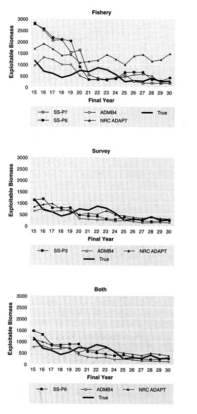
FIGURE 5.17 Comparison of estimated and true biomass (thousand metric tons) in terminal years for 16 retrospective assessments (terminal years 15-30 assessments) conducted on data set 1 using Stock Synthesis (SS-P3, SS-P6, and SS-P7), AD Model Builder, and NRC ADAPT; M was fixed at the true average value in all cases.
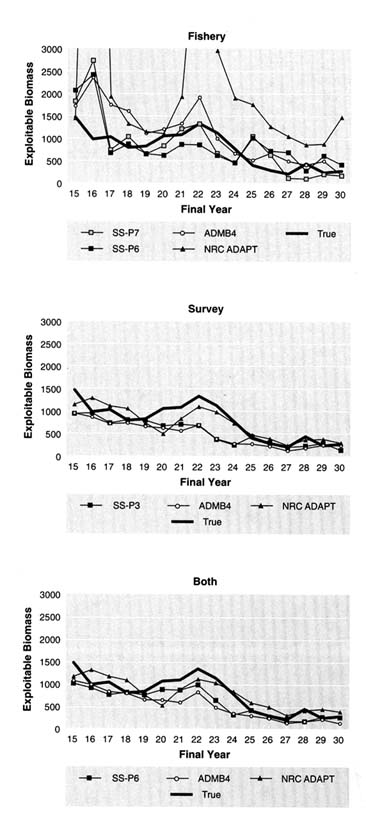
FIGURE 5.18 Comparison of estimated and true biomass (thousand metric tons) in terminal years for 16 retrospective assessments (terminal years 15-30 assessments) conducted on data set 2 using Stock Synthesis (SS-P3, SS-P6, and SS-P7), AD Model Builder, and NRC ADAPT; M was fixed at the true average value in all cases.
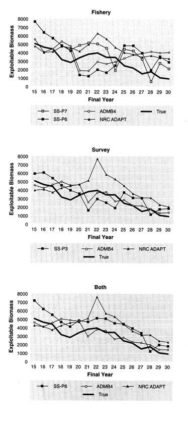
FIGURE 5.19 Comparison of estimated and true biomass (thousand metric tons) in terminal years for 16 retrospective assessments (terminal years 15-30 assessments) conducted on data set 3 using Stock Synthesis (SS-P3, SS-P6, and SS-P7), AD Model Builder, and NRC ADAPT; M was fixed at the true average value in all cases.
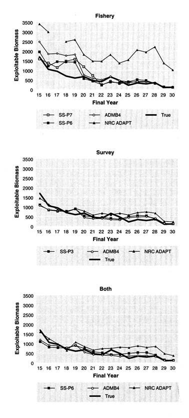
FIGURE 5.20 Comparison of estimated and true biomass (thousand metric tons) in terminal years for 16 retrospective assessments (terminal years 15-30 assessments) conducted on data set 4 using Stock Synthesis (SS-P3, SS-P6, and SS-P7), AD Model Builder, and NRC ADAPT; M was fixed at the true average value in all cases.
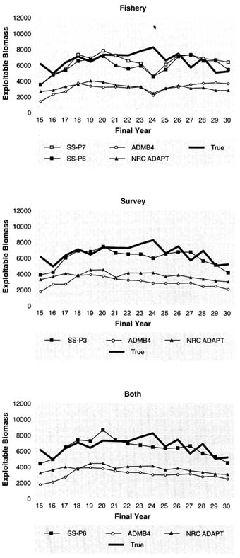
FIGURE 5.21 Comparison of estimated and true biomass (thousand metric tons) in terminal years for 16 retrospective assessments (terminal years 15-30 assessments) conducted on data set 5 using Stock Synthesis (SS-P3, SS-P6, and SS-P7), AD Model Builder, and NRC ADAPT; M was fixed at the true average value in all cases.
TABLE 5.13 Average of Relative Deviations Between Estimate and True Exploitable Biomass in Terminal Year (for terminal years 15-30)
TABLE 5.14 Serial Correlation Between Errors in the Estimates of Exploitable Biomassa in the Terminal Year
TABLE 5.15 Average of Relative Absolute Deviations Between Estimate and True Exploitable Biomass in Terminal Year (for terminal years 15-30)
TABLE 5.16A Number of Assessments with Estimates of Terminal Exploitable Biomass Within ± 25% of True Value
|
|
SS-P6 |
ADMB4 |
NRC ADAPT |
|||||||
|
Data Set |
B |
F |
F |
S |
F |
B |
S |
B |
S |
F |
|
1 |
6 |
2 |
3 |
5 |
4 |
3 |
3 |
4 |
7 |
0 |
|
2 |
9 |
6 |
3 |
8 |
7 |
6 |
5 |
8 |
11 |
2 |
|
3 |
2 |
0 |
1 |
3 |
5 |
10 |
10 |
3 |
3 |
4 |
|
4 |
9 |
5 |
6 |
9 |
7 |
11 |
7 |
6 |
7 |
0 |
|
5 |
16 |
12 |
12 |
14 |
1 |
0 |
0 |
0 |
0 |
0 |
|
NOTE: Maximum n = 16. |
||||||||||
TABLE 5.16B Number of Assessments with Relative Errors in Estimates of Terminal Exploitable Biomass Within ± 50% of True Value
|
|
SS-P6 |
ADMB4 |
NRC ADAPT |
|||||||
|
Data Set |
B |
F |
F |
S |
F |
B |
S |
B |
S |
F |
|
1 |
12 |
6 |
4 |
8 |
6 |
9 |
8 |
12 |
13 |
2 |
|
2 |
14 |
4 |
11 |
14 |
10 |
13 |
13 |
14 |
15 |
3 |
|
3 |
11 |
7 |
6 |
11 |
8 |
13 |
14 |
6 |
6 |
7 |
|
4 |
13 |
10 |
10 |
6 |
11 |
14 |
14 |
7 |
8 |
0 |
|
5 |
16 |
16 |
16 |
16 |
6 |
5 |
5 |
15 |
14 |
8 |
TABLE 5.17 Pearson Correlation Between Relative Deviation and True Change in Exploitable Biomass for Terminal Years 16-30
TABLE 5.18 Percent of Positive Relative Deviations Given a Positive True Change (labeled as an ''up") in Exploitable Biomass for Terminal Years 16-30 Assessments
TABLE 5.19 Percent of Negative Relative Deviations Given a Negative True Change (labeled as a "down") in Exploitable Biomass for Terminal Years 16-30 Assessments
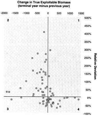
FIGURE 5.22 Example of retrospective error pattern (estimates from model SS-P3[F]) over assessments for terminal years 16-30 and all data sets.
spawner-recruit relationship into age-structured models, as shown in Deriso et al. (1985), which could then be used to calculate MSY and other such parameters. In ADMB, a recruitment model is specified which can include a spawner-recruit relationship. Age-structured models are able to reconstruct annual recruitment values without including a spawner-recruit relationship in the assessment model. In this study, analysts using the delay-difference model did not use a spawner-recruit relationship but instead used a recruitment index derived from the survey. Although the production model used a logistic stock-production relationship, one can construct a form of this model which incorporates a recruitment index. (This was mentioned as a possibility by the analyst but not used, because a recruitment index requires age-structured information and the goal was to see what could be extracted from a simple model). For management, some biological reference points (BRPs, such as F40%) related to spawning biomass per recruit can be calculated without using a spawner-recruit relationship, and such BRPs are being used with increasing frequency in actual assessments. But the spawner-recruit relationship should be investigated to evaluate whether the BRP is appropriate. Whether it is better to do so by incorporating the relationship within the assessment model or as a separate analysis using output from the assessment model is an open question.
Because a full evaluation of stock assessment models could not be done, the committee used its resources to explore the performance of the models in a simulated stock assessment setting in an attempt to (1) evaluate existing methods and (2) suggest new directions of research into stock assessment methods. It is obvious that a more comprehensive evaluation of stock assessment methods should be undertaken, given the results of this study. Issues related to the treatment of measurement and process errors, the functional dependence of population
parameters (e.g., catchability) on biomass, the choice and weighting of individual data sets, information conflicts among data sets, and the appropriate level of model complexity are all unresolved at present, and require attention if there is to be greater confidence in stock assessments. These would be fruitful areas of research.
The committee's analysis indicates that high-quality data, fundamentally the availability of reliable indices to calibrate the models, are essential to produce reliable abundance estimates. In most cases, use of the fishery abundance index resulted in poor performance unless the model contained additional parameters to deal with the trend in the index.
Surplus production and delay-difference models did not perform as well overall as age-structured models; this is not surprising because the simulated data were designed for use with age-structured methods. Surplus production models require a straightforward and immediate response of the population to changes in harvesting levels. The simulated populations were more affected by recruitment fluctuations than by changes in harvest levels. The corruption of indices of abundance by catchability and selectivity changes and by underreporting of catch would make stock assessment with surplus production models nearly impossible. Better results were achieved for delay-difference models because analysts utilized an index of recruitment from the survey and/or fishery data, rather than relying on a stock-recruitment model. Using a knife-edge selectivity assumption in these models when there was an underlying selectivity pattern with age increased the uncertainty and potential bias in estimates of population parameters. Nevertheless, better results were obtained for these models when the survey index was used alone than when only the fishery index or both indices were used.
Among the age-structured models, simple models such as ASA, SS-P3, or NRC ADAPT performed reasonably well when only the survey index was used and when the dynamics of the population and harvest were not too complex. More complex models such as SS-P6, SS-P7, and ADMB4 were sometimes able to handle more complex dynamics and indices with trends. However, the success of these more complicated models depended on correct specification of the dynamic changes in selectivity, catchability, and natural mortality.
Simulation results suggest that models with greater complexity offer promise for improving stock assessment. The Kalman filter (in DDKF) and generalized parametric approach (in AD Model Builder) allowed more realistic treatment of process and measurement errors. The Bayesian treatment of parameters (also in AD Model Builder) provided a means for incorporating uncertainty directly into the analysis and yielded results in terms of posterior probability distributions, which explicitly presented uncertainty. The incorporation of functional dependence of catchability and flexibility in model specification (in SS-P6 and SS-P7) provided a more deterministic way of adding realism. Although no specific model outperformed others in the simulations, the committee was intrigued with how more complex models could reduce, at least partially, the biasing effects related to fishery catchability and selectivity changes.
Simulation results showed that when there is substantial recruitment variability, production models do not perform well. Only with populations that exhibit a strong negative response to fishing should these models be used for routine assessment. Nevertheless, there will be situations in which data limitations preclude the use of other methods. Delay-difference models fared better than production models but worse than age-structured models. Although delay-difference models might be used in situations in which ageing is subject to great error or not possible, it would be more prudent to utilize the age or length information in stock assessments. One of the reasons delay-difference models performed as well as they did in the simulations was use of a recruitment index from the survey. Thus, the development of recruitment indices for use in stock assessments should be considered.
Although the construction of better stock assessment models is likely to lead to better assessments, accurate and precise information about the population is of paramount importance. Although this conclusion is fairly obvious ("garbage in-garbage out"), the simulation study provided a clear illustration of the importance of good data and information. In data set 4, there were few violations of the underlying assumptions used in the assessments, and not surprisingly, most of the stock assessment models performed acceptably. The worst results for this data set were obtained when only the fishery index was used, showing that bad data weaken a stock assessment. Each of the other data sets had some additional complicating factor, that resulted in poorer results than for data set 4. Hence, poor information (e.g., not knowing about a change in catchability) is an additional factor that weakens a stock assessment. When the combination of poor data and poor information becomes large enough (e.g., data set 3), it can be almost impossible to extract any useful stock assessment information.
The major conclusion from the simulation study was that a good index of abundance is needed for useful stock assessment information, not that fishery indices should not be used. Much effort is required to validate any index as a measure of abundance.
Specific examples of poor information incorporated into the simulation study deserve further comment. The misspecification of natural mortality has long been recognized as a critical problem in stock assessment. Overestimation of natural mortality leads to overestimation of both population abundance and optimal harvesting rate due to yield-per-recruit consequences. In the simulation study, natural mortality was rarely overestimated. Rather, the variability in natural mortality made it difficult to estimate other parameters. Two possible approaches to incorporating variable natural mortality are (1) to pursue methods such as multispecies virtual population analysis (MSVPA), that utilize data on food habits of different species, and (2) to use Bayesian specification of priors for natural mortality, provided that appropriate priors can be found (e.g., through meta analysis).
Underreporting in data set 2 led to underestimation of population biomass, with greater effects at the beginning of the data series. Thus, the proportionate decline in population over time was underestimated, which could lead managers to think that less strict harvesting policies are adequate to rebuild a depleted population. The obvious solution is to design the catch-reporting system so that underreporting is less likely to occur (see Chapter 2). It is notable that underreporting can work to the detriment of fishers in the long run by corrupting the data used in assessment models.
The decline in age selectivity in data sets 1, 2, and 3 resulted in a fishery index that would be higher than under constant selectivity, because more younger fish would be harvested and added to the fishery index. Such a change could occur by targeting of smaller fish as a population became depleted or by a change in the age selectivity curve due to density-dependent or environmentally induced changes in growth. Collection and analysis of growth data are critical to understanding changes in age selectivity. If changes can be detected from such observations, modeling can readily account for them, either by utilizing length-based methods or by having separate sets of age selectivity parameters (e.g. in SS-P7 or ADMB).
The change in survey catchability in data set 3 created a situation in which neither index of abundance was proportional to biomass. When a change in catchability was incorporated into the models, its value could be estimated in many cases, with a resultant improvement in stock assessment results. If the committee had not told the analysts of the potential change, however, it is doubtful whether it would have been detected. The implication is that calibration of survey catchability is an important consideration; calibration studies should be done when there are changes in vessels, crews, or operations that affect the way a survey is conducted (see ASMFC, 1997).
Retrospective analyses from the simulation revealed that stock assessments can vary substantially from the true values over time. These analyses also illustrated that the departures of estimated stock biomass from true values can persist in one direction over time. Consequently, management actions could have deleterious effects on the population long before they are observed. Thus, conservative harvest policies should be developed. The committee encourages greater use of retrospective analysis in stock assessment. The results can suggest when model misspecification is occurring and when data sources are providing contradictory information. The retrospective analysis reported herein focused on an evaluation of modeling. Another type of retrospective analysis involves summarization of previous stock assessment results regardless of which model was used. This type of retrospective analysis can be useful in examining the stability of the stock assessment process as actually implemented.
The additional investments in stock assessment research recommended by the committee require additional commitments of personnel, field research, and analytical research. Chapter 4 contains a discussion of where investments should be made—not merely in collecting more of the same information but in improving the type of information collected as well. Simulation results suggest that if such investments cannot be made, some stock assessments will be far from the truth periodically, and consequently that management mistakes leading to fish population collapses and other negative consequences will be made.
The approach of having a committee conduct simulation research involving NMFS scientists in an independent review of stock assessment methods is not undertaken frequently. This approach was quite useful for brainstorming issues related to stock assessment, and new understanding and novel approaches to stock assessment were inspired by this project. This work was designed to evaluate not the individual NMFS scientists
involved but the methods used in stock assessment. Nevertheless, it took a great deal of courage for these scientists to participate, and the committee was impressed with the analysts' willingness and ability to provide what it requested, their creativity in applying existing methods and developing new ones, and their fortitude in taking on a difficult assignment in addition to their regular duties. To foster excellence in stock assessment, NMFS should continue to support and encourage scientists to engage in creative stock assessment activities (e.g., workshops, gaming sessions, and conferences) so that the process of doing stock assessment does not become routine and stale.


