
Proc. Natl. Acad. Sci. USA
Vol. 94, pp. 8300–8307, August 1997
Colloquium Paper
This paper was presented at a colloquium entitled “Carbon Dioxide and Climate Change,” organized by Charles D. Keeling, held November 13–15, 1995, at the National Academy of Sciences, Irvine, CA.
Characteristics of the deep ocean carbon system during the past 150,000 years: SCO2distributions, deep water flow patterns, and abrupt climate change
E DWARD A. BOYLE
Department of Earth, Atmospheric, and Planetary Sciences, Massachusetts Institute of Technology, Cambridge, MA 02139
ABSTRACT Studies of carbon isotopes and cadmium in bottom-dwelling foraminifera from ocean sediment cores have advanced our knowledge of ocean chemical distributions during the late Pleistocene. Last Glacial Maximum data are consistent with a persistent high-SCO2state for eastern Pacific deep water. Both tracers indicate that the mid-depth North and tropical Atlantic Ocean almost always has lower SCO2levels than those in the Pacific. Upper waters of the Last Glacial Maximum Atlantic are more SCO2-depleted and deep waters are SCO2-enriched compared with the waters of the present. In the northern Indian Ocean, d13C and Cd data are consistent with upper water SCO2depletion relative to the present. There is no evident proximate source of this SCO2-depleted water, so I suggest that SCO2-depleted North Atlantic intermediate/deep water turns northward around the southern tip of Africa and moves toward the equator as a western boundary current. At long periods (>15,000 years), Milankovitch cycle variability is evident in paleochemical time series. But rapid millennial-scale variability can be seen in cores from high accumulation rate series. Atlantic deep water chemical properties are seen to change in as little as a few hundred years or less. An extraordinary new 52.7-m-long core from the Bermuda Rise contains a faithful record of climate variability with century-scale resolution. Sediment composition can be linked in detail with the isotope stage 3 interstadials recorded in Greenland ice cores. This new record shows at least 12 major climate fluctuations within marine isotope stage 5 (about 70,000–130,000 years before the present).
On time scales exceeding millennia, the ocean carbon system regulates atmospheric CO2 levels. The gas trapped as bubbles in polar ice cores shows that CO2 levels varied between 190 and 280 ppmV during glaciation cycles and, hence, that some aspects of the oceanic carbon system are naturally variable. Several ideas on how the ocean produces these changes in atmospheric CO2 have been advanced. Although many ideas have merit because they call attention to processes that regulate atmospheric CO2, it has proven difficult to come up with a widely accepted model for the dominant cause of glacial/interglacial CO2 variability.
Despite this persistent sticking point, significant progress has been made concerning the distribution of metabolically regenerated CO2 throughout the deep ocean. The past state of the oceanic CO2 distribution is recorded by carbon isotopes and phosphorus-analog Cd as they are incorporated into shells of benthic foraminifera preserved in deep-sea sediments. Marine organic matter is enriched in 12C and Cd, so that surface waters are depleted in 12C and Cd because of their removal by plant growth, and deep waters are enriched in 12C and Cd as debris from those plants (and animals that eat them) decompose in deeper waters. From global data on the distribution of metabolic CO2 and its analogs, we can infer characteristics of thermohaline spreading patterns.
This paper will first briefly review significant aspects of Last Glacial Maximum (LGM) ocean chemical distributions in major ocean basins, emphasizing major areas of agreement and discordance, and then tie this evidence together into a unifying hypothesis for LGM deep-ocean circulation patterns. The paper concludes with new evidence concerning century-scale variability of North Atlantic climate during the past 150,000 years (15 kyr).
LGM Nutrient Distribution in Deep Waters of Major Ocean Basins: A Brief Overview
Eastern Tropical Pacific. A consensus view has dominated the past decade. Foraminiferal LGM d13C was -0.3% lower than the level in the Holocene in the benthic foraminifera Uvigerina and Cibicidoides wuellerstorfi in the eastern tropical Pacific. This shift has been interpreted as due to a whole-ocean shift in d13C caused by oxidation of continental organic matter during glacial periods (1, 2, 3, 4, 5 and 6). LGM benthic foraminiferal Cd/Ca was about 15% lower in the same region; this lowering has been attributed to higher Cd in the LGM Atlantic oceana (assuming a constant oceanic Cd inventory) (3, 6, 7). Both interpretations agree that this region remained near the end of the “conveyor belt” with high SCO2 due to its accumulation as sinking particles decompose.
Two recent reports have uncovered potential problems with this widely adopted consensus. First, laboratory culturing experiments on planktonic foraminifera suggest that foraminiferal d13C may be sensitive to pH (8); if the same sensitivity holds for benthic foraminifera and if pH of the LGM ocean rose as much as indicated by early reports on LGM “paleo-pH” [based on foraminiferal d11B (9, 10)], then a significant portion of the eastern tropical Pacific d13C signal could be due to changes in pH rather than a whole-ocean d13C shift due to continental organic matter oxidation (11). Second, it has been noted that the oceanic Cd inventory is sensitive to changes in the extent of reducing conditions, where CdS precipitates from sedimentary pore waters (12, 13). Depending on assumptions, a portion of lower Cd in the eastern tropical Pacific could be caused by enhanced removal of Cd from the ocean during glacial times rather than by a shift of Cd into other water masses. Neither argument can be considered established, however, so the current consensus may well survive.
North and Tropical Atlantic. Despite some early substantial disagreements, for the past 5 years the consensus view of LGM Atlantic paleochemistry has been that there was 13C enrichment/Cd depletion of upper tropical and North Atlantic waters (1–2 km) and 13C depletion/Cd enrichment in deeper waters (3, 4, 5 and 6
|
|
© 1997 by The National Academy of Sciences 0027-8424/97/948300-8$2.00/0 PNAS is available online at http://www.pnas.org. |
km) (3, 4 and 5, 14, 15 and 16). This distribution has been attributed to a shoaling of high 13C/low Cd North Atlantic source waters compensated by a greater influx of low 13C/high Cd Antarctic bottom waters. This replacement of some NADW by glacial Antarctic bottom water (AABW) notwithstanding, mid-depth northern Atlantic waters (˜3 km) have higher 13C and lower Cd than do waters of the eastern tropical Pacific. The structure and temporal variability are complex in detail (17). Whether the LGM NADW conveyor belt was global in scope as it is today has been debated considerably (see ref. 18 for my recent review of this debate). The matter may have been settled recently by studies of 231Pa/230Th by Yu et al. (19). 231Pa generated from decay of 235U in the Atlantic is “missing” from Atlantic sediments. Yu et al. make a convincing case that this deficiency is due to NADW-borne transport of 231Pa out of the Atlantic into the Antarctic Circumpolar Current, where 231Pa is trapped into sediments at levels exceeding its regional production rate. Because this deficiency persists during the LGM, the conveyor must have continued to move 231Pa out of the Atlantic.
Northern Indian Ocean. Kallel et al. (20) reported that upper waters of the northern Indian Ocean had higher levels of 13C than those at present. Naqvi et al. (21) questioned this interpretation because it was based upon a Geochemical Ocean Sections/LGM comparison rather than a core top/LGM comparison (because there are significant differences between Geochemical Ocean Sections d13C and core top C. wuellerstorfi d13C). More recently, foraminiferal Cd evidence from several species of aragonitic and calcitic benthic foraminifera was presented (22); this evidence shows that upper northern Indian Ocean nutrient depletion (strongest in the Arabian Sea) could be reconciled with the evidence of Naqvi et al. (21).
The major problem following this observation is the difficulty in accounting for the cause of 13C enrichment/Cd depletion. The Red Sea cannot be the source because its sill was too shallow during the LGM (due to sea level depression). Other sources (Indonesian basins, Antarctic sources) cannot be ruled out entirely but seem unlikely. In the “Global Picture” below, I suggest that upper glacial North Atlantic intermediate/deep water (GNAI/DW) is the source of this low SCO2 water.
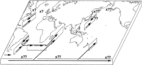
FIG. 1. Schematic diagram of global deep water circulation during the LGM. Parallelograms represent hydrographic sections, divided into upper deep and lower deep circulations, as indicated by arrows. x, marks a possible site of sinking; ?, a certain regional source whose specific formationsite is unknown; ??, a questionable source.
Antarctic. The Antarctic has been a major sticking point for deep water paleoceanography. Most published LGM d13C data show values that are much lower than those of today (in some cases lower than anywhere else in the ocean) (4, 23, 24 and 25). Cd evidence is also self-consistent but contradictory to d13C evidence: Cd is either the same as it is today or slightly lower (7, 23, 24). So d13C data indicate that Southern Ocean deep water was high in SCO2, whereas Cd data indicate that it was moderate or lower in SCO2. The d13C evidence also is difficult to reconcile with lowered glacial atmospheric pCO2 (25). Attempts have been made to resolve this conundrum. These explanations can account for part of the discrepancy but not all (26). I have reviewed this situation recently (24) and argue that the Southern Ocean “Mackensen Effect,” whereby d13C of C. wuellerstorfi is observed to be low under waters of high productivity (27), is stronger during the LGM, hence 13C data are too low. However, this solution is not universally agreed to by stable isotope paleoceanographers.
Northwest Pacific. The northwest Pacific has been another difficult area; however, in this case the problem includes internal inconsistency for each tracer as well as tracer-to-tracer discrepancies. Some evidence is consistent with formation of a low-S,CO2 LGM deep water [e.g., Cd is consistently lower in LGM benthic foraminifera at all depths compared with levels in the eastern tropical Pacific (7), but the few available core top Cd measurements in this region are inexplicably low (7, 28)]. Some northwest Pacific sites show d13C similar to that found in the eastern tropical Pacific (29), but other sites show values that are enriched in 13C (4).
Global Picture. On the broad scale considered here, LGM deep water paleochemical studies have three hits and two misses: Cd and d13C data are consistent and informative on LGM chemical distributions in the eastern tropical Pacific, North and equatorial Atlantic, and northern Indian Ocean, but disagree substantially in the Southern Ocean and northwest Pacific. If the Southern Ocean disagreement is attributed to a productivity-related artifact in d13C (and Cd evidence is accepted), and if the northwest Pacific is left as an open question, a synthesis of LGM paleochemical data can be offered as a testable hypothesis (Fig. 1). In Fig. 1 , major flows are represented in “sections” along western boundaries of major ocean basins, with flow divided into upper deep and lower deep sections (approximately 1.5–2.5 and 2.5–5 km). Areas where bottom water is possibly formed, formation regions that are uncertain as to exact location but must have occurred within some broad region, and formation regions that are possible but
not necessarily required are marked in Fig. 1 . It is assumed that recirculation flows fill the basin interiors.
The most important and well documented change in this LGM global circulation is the shift of CO2-depleted NADW to shallow depths, replaced in the deepest waters by a northward flow of high-CO2 Antarctic water. The exact source area of this NADW is not known but is certain to be found somewhere in northern reaches of the Atlantic. Because the 231Pa/230Th data of Yu et al. (19) require a net export of water from the Atlantic, this shallow GNAI/DW must penetrate into the Antarctic Circumpolar Current. As suggested by Toggweiler et al. (30),
a shallower variety of North Atlantic deep water will have a more difficult time reaching high latitudes of the Southern Ocean where it can be recycled into the bottom water. . . . Instead, any high-13C water emerging beyond the tip of Africa might simply flow eastward into the Indian and Pacific basins, bypassing the Antarctic entirely.
Although persistently low Cd in Antarctic deep waters is evidence against complete elimination of an Atlantic influence on Antarctic deep water chemistry, there nevertheless should be a tendency for less effective southward penetration of a shallower GNAI/DW. Extending Toggweiler’s logic, I suggest here that much of the GNAI/DW that enters the northern portion of the Antarctic Circumpolar Current folds around the southern tip of Africa and moves northward as a western boundary current in the 1–2 km depth range. This flow can explain the low-SCO2 waters in the upper waters of the northern Indian Ocean. This circulation pattern also explains why the LGM Arabian Sea—proximate to the western boundary source—is lower in SCO2 than the Bay of Bengal, which has older recirculated waters.
Part of the circulation scheme must remain vague because of data inconsistencies. However, northward penetration of highSCO2 water from the Antarctic into the North Atlantic attests to formation of glacial AABW somewhere. There is little evidence on where in the Antarctic this glacial bottom water forms. Today, most primary AABW forms in on the continental shelf in the Weddell Sea with a lesser contributions from the Ross Sea and other sources (31). LGM sea level lowering of 120–130 m (32) and probable northward extension of year-round sea ice (33) may weaken this source. Other sources of AABW may replace the Weddell Sea; the Ross Sea and Southern Indian Ocean are possible replacements. Michel et al. (34) and Rosenthal (23) have suggested that bottom water formation may occur in the Indian Ocean sector, although they envision quite different initial properties. Michel et al. argue for formation of high-SCO2 bottom water (based on very light LGM foraminiferal d13C observed in the Indian sector), whereas Rosenthal argues for nutrient-depleted deep water formation (based on Cd evidence).
Wherever this Antarctic water forms, it must also enter the Pacific as it does today. The major question for LGM Pacific circulation is whether this AABW simply ages and returns southward as deep water (as it does today) or is supplemented by additional sources in the North Pacific. When possible sites of formation are mentioned, the Sea of Okhotsk and Bering Sea figure prominently. If deep water forms, it may be an upper level intermediate/deep water as seen in the glacial North Atlantic.
Although there are loose ends to this story, a coherent picture of LGM Atlantic and Indian Ocean chemical characteristics can be fashioned from simple premises. For these regions, the scientific challenge is to fill in details of this picture and test it against other observations, such as 14C ventilation rates. In other regions, major advances are required to develop even a simplified picture of the circulation; however, some initial targets are obvious. (i) Why do d13C and Cd disagree with one another in the Southern Ocean? (ii) Can a coherent picture of chemical distributions in the northwest Pacific be fashioned from either tracer?
Rapid Climate Variability in the North Atlantic
High Resolution Climate Change in the Ocean: A Brief Review. Just as we have a much more detailed picture of LGM chemical characteristics and inferred circulation of the Atlantic, we also have a better view of temporal variability of these characteristics. On longer time scales, paleochemical indicators show clear influence of Milankovitch 100–41-23 kyr orbital cycles; the Spectral Mapping Project (SPECMAP) investigated the relation of deep water cycles to orbital forcing and other responses in the climate system (30, 35). On shorter time scales, there is growing interest in decadal-millennial deep water variability. Greenland ice core evidence (36, 37, 38 and 39) shows that climate can shift abruptly between warmer and colder states. Broecker and colleagues ( 40, 41 , 42 , 43 , 44 , 45 , 46 , 47 and 48 ) have suggested that global deep water conveyor belt flow may be a prime driver of these changes, and hence there is significant effort directed at establishing deep water changes at high temporal resolution within an accurate time scale.
The major challenge in this effort is that temporal resolution is limited by the low sedimentation rate of deep-sea sediments (typically only a few centimeters per thousand years) and biological reworking of the upper several centimeters of sediment. To study events shorter than millennia, it is necessary to work in regions of unusually high accumulation rate. Higher accumulation rates occur on continental margins, although slumps and other sedimentary disturbances occur almost as frequently, making it difficult to find undisturbed sections. High accumulation rates also occur in deep-sea “drift” deposits, where preferential scouring of fine-fraction material over a broad region combines with preferential deposition where transport weakens. Although these deposits are not common, in the North Atlantic there is at least one drift deposit at the depth of every major water mass and source. Hence, the search for short-term ocean climate variability has focused on these drift deposits as well as special regions of continental margins where undisturbed deposition can be documented [e.g., Cariaco Trench (49), Santa Barbara Basin ( 50 ), and others].
“Dansgaard-Oeschger” Interstadial events clearly recorded in Greenland ice cores are matched by events in foraminiferal species abundances North Atlantic cores (51, 52). Although the chicken–egg question of cause and effect is not resolved yet, a linkage between abrupt climate variability in Greenland and the surface North Atlantic is clearly demonstrated. The degree to which deep Atlantic circulation is involved is an open question. In the northern Atlantic where these events have their strongest expression in surface water properties, deep water paleochemical signals can be small even for extrema such as the LGM (18, 53), and benthic foraminifera are often scarce and sporadic, making it hard to construct a continuous high-resolution time series at these sites. Curry and Oppo (68) has evidence suggesting that at least the larger of these events influences the carbon isotope composition of benthic foraminifera from the tropical Atlantic. To answer the question more definitively, a benthic paleochemical record from a very high deposition site with a precise and accurate chronology is required.
Bermuda Rise Paleoclimatology. For several years now, Lloyd Keigwin and I have worked on drift deposits of the Bermuda Rise, where accumulation rates vary from 10–20 cm/kyr (during warm climate periods) to 100–200 cm/kyr (during extreme glaciation). Located some 335 km northeast of Bermuda, sedimentation in this region is enhanced by fine-grained material eroded from the North American continental margin and transported to this site by energetic bottom currents (which weaken and allow fine-grained sediment to settle out). The bottom currents focus fine-grained sediments (clays, other detrital sediments, and coccoliths) onto this site (enhancing the accumulation rate several-fold), whereas coarse-grained materials such as planktonic and benthic foraminifera accumulate at a normal oligotrophic ocean rate (54, 55 and 56). The high accumulation rate increases temporal resolution and allows for an examination of
century-scale (and shorter) climate variability. In addition to high temporal resolution, the Bermuda Rise has two other characteristics that make it appropriate for study of ocean climate changes. (i) It lies beneath oligotrophic subtropical waters, allowing it to serve as a representative of a large and typical ocean province; few other drift deposits are so located. (ii) The bottom depth is >4,400 m, giving benthic foraminifera a sensitive perspective on changes in lower North Atlantic deep water. Dilution of coarse-grained foraminiferal signal carriers has the disadvantage, however, that drift deposits require much larger sample sizes.
Keigwin and Jones provided a precise accelerator mass spectrometry 14C-based chronology for the upper portion of the Bermuda Rise (57, 58); below the zone of radiocarbon dating, correlation of features in the benthic oxygen isotope curve to the orbitally tuned SPECMAP time scale extends the time scale. Analysis of the percentage of CaCO3 (%CaCO3) at this site (58) and at another drift deposit on the Bahamas Outer Ridge shows typical Atlantic warm high-carbonate/cold low-carbonate pattern. High temporal resolution reveals numerous millennial-scale events that are similar in frequency, timing, and pattern to “interstadial” events observed in the Renland (Greenland) ice core (58). Finally, in a study of the most recent deglaciation, Keigwin and I (15, 59) showed that surface and deep water properties are punctuated by a series of at least four millennialscale events. The most recent of these events is the “Younger Dryas” cooling, which occurred 13,000–11,500 calendar years ago, where both benthic Cd and d13C indicate a strong and clear diminution of the percentage of low-SCO2 lower NADW. This evidence supports the idea of a linkage between thermohaline circulation and abrupt cooling during the Younger Dryas. The middle two Cd events coincide with pulses in freshwater fluxes into the Gulf of Mexico during deglaciation, and the earliest Cd event coincides with the most recent “Heinrich Event” pulse of detritus from icebergs into the northern North Atlantic. Hence this limited study of surface and deep water characteristics—combined with the extended record of %CaCO3—suggests that abrupt variability may be a major characteristic of subtropical surface and deep waters during glaciations and deglaciations.
This case study of deglaciation provides evidence for millennial-scale climate variability during glaciations and deglaciations, but there is more significant public policy concern about the possibility of abrupt changes during warm climate periods. This concern was amplified by the report that extreme abrupt events characterized the last interglacial (“Eemian” or oxygen isotope stage “5e”) in the central Greenland Ice Project (GRIP) ice core (37). Subsequently, concerns were raised about the fidelity of deeper portions of the GRIP record because (i) the interval in question is not replicated in the nearby Greenland Ice Sheet Project 2 (GISP2) ice core, (ii) inclined beds (and probable folding disturbances) are seen in the GISP2 core, suggesting that the deepest portions of ice cores near bedrock are subject to stratigraphic disturbances, and (iii) there is no sensible correlation of air bubble d18O2 record in deeper parts of both GISP2 (60) and GRIP (61) ice cores with that in the stratigraphically impeccable Antarctic Vostok ice core (62), suggesting that neither Greenland ice core contains a continuous undisturbed Eemian sequence. However, concern raised by the original report made it evident that we have very little detailed paleoclimatic information from previous warm interglacial periods, such as the Eemian. Although there are valid grounds for doubting GRIP Eemian fluctuations, little is known about the stability of stage 5e at high temporal resolution. Hence a surge of activity has been directed at the last interglacial period.
Long Sediment Cores for Decadal- to Century-Scale Paleoclimatology. Because this question requires high temporal resolution, sediment drift deposits such as the Bermuda Rise are prime targets for studies of ocean climate characteristics of the last interglacial period. However, the desirable high sedimentation rates create a major problem; on the Bermuda Rise, the last interglacial period is beyond reach of most piston cores, which are rarely longer than 20 m, and more typically are considerably shorter. Deeper sediments can be obtained by the Ocean Drilling Project, but these come as narrow-diameter, discontinuous, 9-m sections. Recently, a superior alternative for studying sediment in the 20- to 50-m (below seafloor) depth zone has been developed. Working on the large French supply/research vessel Marion Dufresne, Yvon Balut has developed a capability for taking cores longer than 50 m with a giant large-diameter Kullenberg-style piston corer. The capability draws upon vessel size and shape (the new Marion Dufresne is 120.5 m long with a displacement of 10,380 metric tons, and has a long straight starboard working rail), a highcapacity (18 tons) kevlar-cable winch, and a unique core handling system that allows for the deployment of 60-m-long core barrels. One such core, 51.7 m long, collected in the Indian Ocean in 1990 has already been described (63). Inspired by that success, a proposal was initiated in 1992 to bring the ship to the Bermuda Rise to obtain a high-resolution record of the last 15 kyr. The funding contribution from this U.S. National Science Foundation project was then combined with other international projects (with financial contributions from Canada, Germany, Britain, and France, as well as scientific personnel contributions from several other countries) to form the 1995 “IMAGES” coring expedition throughout the North Atlantic Ocean.
During a 22-h period in the vicinity of the Bermuda Rise, three cores were collected during this program: MD95-2034 (47.2 m long, obtained in a 60-m core barrel), MD95-2035 (39.2 m long, obtained in a 40-m core barrel), and MD95-2036 (52.7 m long, recovered in a 60-m core barrel). MD95-2034 (33°41.46'N, 57°34.54'W, 4,461 m uncorrected) and MD95-2036 (33°41.44'N, 57°34.55'W, 4,461 m uncorrected) were collected at essentially the same site, and MD95-2035 (33°29.195, 57°53.157, 4,286 m uncorrected) was collected southeast of the other two cores in an area of somewhat lower deposition. Shipboard measurements of whole-core magnetic susceptibility, GRAPE (gamma ray absorption porosity estimation), and sound velocity were made. Cores MD95-2034 and MD95-2035 were split on board, photographed, and described, and their optical reflectance spectral properties were logged by a Minolta CM 2002 spectrophotometer with a 1-cm-diameter spot size which records 31 bands from the 400- to 700-nm wavelength. It was evident from shipboard magnetic susceptibility records that MD95-2034 and MD95-2036 were essentially identical apart from a few coring disturbances in upper sections. From reflectance spectrometry, a preliminary stratigraphy was developed for MD95-2034 as described below, the stage 5e section of MD95-2034 identified, and then the matching stage 5e section in MD95-2036 was identified by matching magnetic susceptibility profiles. This section of MD95-2036 was then split on board, optical reflectance were recorded, and then sampled were taken at 1-cm intervals; burrows and other disturbances that were visually evident were avoided. These samples were brought back to Massachusetts Institute of Technology within a week of coring, and they were immediately processed to begin foraminifera picking for isotope and geochemical analysis.
Optical Spectrophotometry of Bermuda Rise Cores: Introduction. Because dominant contributors to optical characteristics of sediments in this region are calcium carbonate (white) and clays (dark), visible light reflectance is a function of sedimentary %CaCO3. As shown by Keigwin and Jones (58), %CaCO3 at this site records millennial-scale climate events with high resolution. Hence, optical reflectance spectrophotometry is of great utility in establishing stratigraphy of cores in this region. By matching chemically measured %CaCO3 records from the previous longest core from this site (KNR31-GPC5, 29 m) and optical reflectance records, the stratigraphy of these new cores can be quickly established. Beyond the interval covered by KNR31-GPC5, it is expected that the boundary between the last interglacial stage 5e and the previous glacial maximum (isotope stage 6) will be
marked by a strong decrease in %CaCO3 (as on the transition between LGM and Holocene). By this means, an approximate stratigraphy could be built up quickly on board ship, allowing the crucial stage 5e section to be identified and sampled immediately.
Although spectral reflectance data can be represented in many different ways, in this work data will be presented using the Commission Internationale de l’Eclairage “Lab” system, which represents spectral data as three parameters that approximate a subjective linear human physiological visual response to overall lightness (L, higher numbers are brighter), red-to-yellow balance (a, higher numbers are more red than yellow), and yellow-to-blue balance (b, higher numbers are more yellow than blue) (64). On the Bermuda Rise, as noted above, the dominant spectral signature is the overall lightness signal created by changes in relative proportion of white CaCO3 and dark clays. The color variables a and b are interesting because the Bermuda Rise receives variable fluxes of hematite originally eroded from Canadian Maritime Province Permo-Carboniferous red beds, which impart a reddish hue to the sediments (“brick-red lutite”) (65). Variability of this component differs significantly from that of CaCO3 and, hence, provides independent information on climate change.
The comparison of spectral lightness (L) for cores MD95-2034 and MD95-2036 with the %CaCO3 record of KNR31-GPC5 shows close correspondence of spectral reflectance to features of the %CaCO3 record (Fig. 2). This correspondence is most apparent in the interval from isotope stage 3 to stage 5a (1,700–2,800 cm in KNR31-GPC5; 1,700–3,600 cm in MD95-2034; and 1,900–3,900 cm in MD95-2036). This rapid and simple shipboard measurement provides as much stratigraphic information as the slower %CaCO3 measurements. Examination of lightness records leaves little doubt that both MD95-2034 and MD95-2036 contain complete records of marine oxygen isotope stage 5 and a considerable portion of isotope stage 6.
The upper portion of MD95-2034 was disturbed during core recovery, as was MD95-2036 to a lesser extent, so comparison between lightness and %CaCO3 is less helpful in this interval. The greatly extended isotope stage 2 (where accumulation rates are 100–200 cm/kyr) is relatively featureless as represented here, but it should be noted that when freshly split, this interval contained many black bands that are relic Zoophycos horizontal burrow structures containing sulfides which are unstable in the presence of oxygen (Fig. 3). These black bands fade within hours of exposure to the atmosphere. To eliminate these stratigraphically irrelevant structures, the spectrophotometer operator avoided these structures and attempted to find spots that were more representative of sediment typical of a 5-cm interval.
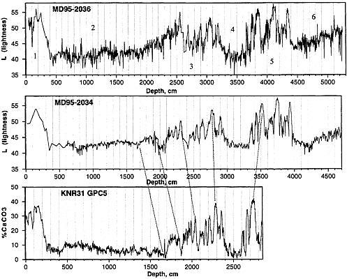
FIG. 2. Comparison of spectrophotometric reflectance (L) data from MD95-2034 and MD95-2036 with the %CaCO3 record from KNR31-GGC5 (58). Numbers on the MD95-2036 plot are marine oxygen isotope stages (centered in respective stages). Note the close correspondence of optical and chemical fluctuations between cores.
The L lightness fluctuations of MD95-2034 and MD95-2036 are shown in Fig. 2; these records are highly similar. The apparent differences arise because (i) the average sample spacing for MD95-2034 was 5.1 cm, whereas that for MD95-2036 was 3.3 cm (this is the main factor causing visually apparent differences; by sampling more frequently, finer-scale variability and analytical noise become more evident); (ii) except for three sections containing and adjacent to stage 5e, MD95-2036 was measured using the 3 mm × 4 mm Colortron spectrophotometer, whereas all of MD95-2034 was measured with the 1-cm-diameter Minolta spectrophotometer (the smaller spot size contributes to higher variability); (iii) MD95-2034 was split on board, and spectra were measured immediately; MD95-2036 was transported back to Massachusetts Institute of Technology, and splitting and spectral measurements were made several months after sample collection. This difference between cores split on board and later on shore probably does not significantly affect color records, as can be seen by a detailed comparison of isotope stage 5 color records from MD95-2034 (shipboard spectrophotometry) and MD95-2036 (spectrophotometry months after coring for the 3,600- to 4,200-cm interval).
The oxygen isotope stage 5 reflectance records of MD95-2034 and MD95-2036 are compared on simple linear depth scales in Fig. 4. Apart from slight scale differences, records are nearly identical down to the centimeter scale; slight adjustments of depth
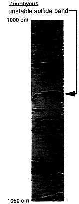
FIG. 3. Video image of one section of MD95-2036 from isotope stage 2 containing Zoophycos relic structures. Several bands occur within this interval; only the most prominent one is marked by the arrow.
control points would make it difficult to discern that two different records were plotted. This evidence attests to the fidelity of both records in recording regional sedimentation characteristics unmarred by burrowing or local stratigraphic disturbances. This comparison also shows that there is no significant accuracy offset between the two spectrophotometers and that no artifactural color changes occurred during storage of and transport of the unsplit sections of MD95-2036.
Optical Spectrophotometry of Bermuda Rise Cores: Paleoclimatological Implications. Fig. 5 compares reflectance properties of all three of the new Bermuda Rise cores. Because MD95-2034 was collected at a site of slightly lower sedimentation rate, it contains a record of longer duration despite its shorter length, extending back to isotope stage 10. It can be seen that all of these cores display high resolution approaching century time scales and that patterns are similar for each core. This comparison also provides a dramatic example of the effect of bioturbation where some detail evident in higher accumulation rate cores (which average about 27 cm/kyr for their entire record lengths) is lost in a core with an average sedimentation rate of “only” 11 cm/kyr.
Data from MD95-2034 were mapped onto a preliminary time scale using radiocarbon and oxygen isotope dates from KNR31-GPC5 (58) supplemented by the assumption that the grayscale transition at the beginning of isotope stage 5 corresponds in age to the SPECMAP 6.0 oxygen isotope marker (Termination II) and that to a first approximation—certainly not true in detail—sedimentation is uniform in stage 5. These records can then be compared with ice core data from Greenland and Antarctica using ice core time scales developed by Bender et al. (60) (Fig. 6). Although temporal correlations will require further critical examination and development of a benthic oxygen isotope record for the earlier portion of the Bermuda Rise, at a first glance one can see continuation of the rich structure and correlation with number and timing of Renland ice core interstadials that Keigwin
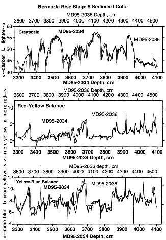
FIG. 4. Detailed comparison of spectrophotometric reflectance (Lab) data from MD95-2034 (thick line) and MD95-2036 (thin line) during isotope stage 5. Both cores are plotted on (different) linear depth scales, with no stretching of sections.
and Jones noted for stages 3 through 5a. With a more detailed isotope record from GRIP and GISP2, these climate correlations can now be extended to specific tentative correlations between interstadial events and CaCO3 cycles and extended to the earlier interval of isotope stage 5. Clearly, the %CaCO3 climate record at this site (as seen through spectral reflectance) reveals more structure than the less structured marine isotope 5a–e partition based on lower accumulation rate cores (67). Isotope stage 5 shows at least 11 identifiable subdivisions. The most recent of these correspond to Greenland Interstadials 19, 20, and 21. The earliest of these %CaCO3 peaks correspond to the beginning of marine stage 5e (based on preliminary d18O analyses by L. D. Keigwin, personal communication) and probably also to the early “hump” in the Vostok dD record. Based on the same preliminary d18O data, the sudden %CaCO3 drop at the end of this peak also appears to lie within the warm portion of isotope stage 5e. Ice core data from Greenland and Antarctic and these new Bermuda Rise records argue for a more complex climate variability during marine oxygen isotope stage 5.
This %CaCO3 (reflectance-based) variability in this region dominantly reflects a variable input of clay superimposed on a relatively constant calcium carbonate influx (56). Hence, these fluctuations are likely to be related to climate processes that affect clay flux into the western North Atlantic basin, including erosion on land and the continental rise, and transport by rivers and deep currents. Addition evidence for abrupt century-scale variability during stage 5 is seen in the a red-to-yellow color balance variable (Fig. 4). This parameter reflects transport of hematite from the Canadian Shield red beds, a transport that is clearly quite different from transport of clay minerals. For example, during the abrupt fall of
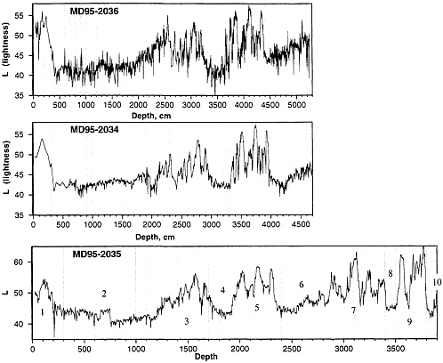
FIG. 5. Comparison of spectrophotometric reflectance (L) data from MD95-2034, MD95-2036, and MD95-2035. Note that MD95-2035 extends to isotope stage 10 because of its lower sedimentation rate. Numbers on MD95-2035 plot are marine oxygen isotope stages (centered in respective stages).
%CaCO3 in mid-stage 5e, the hematite content rises abruptly for a few centuries and then falls back to its previous level, even though %CaCO3 remains low for much longer.
Studies of the isotopic composition of planktonic and benthic foraminifera and Cd/Ca variability of benthic foraminifera are now underway. Early results suggest that the level of
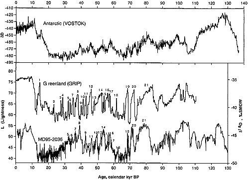
FIG. 6. Comparison of spectrophotometric reflectance (L) data from MD95-2034 with central GRIP d18O data ( 37) and Antarctic Vostok dD data (66) (ice cores being plotted on time scales developed by the authors of refs. 60 and 62. Note that although the SPECMAP marine d18O record is reference for all time scales (beyond the range of layer-counting and radiocarbon measurements), time scales are independently developed by correlation to major features that are not well developed during isotope stage 3. Hence, relative errors of several thousand years may occur for any one of these time scales, and it is not expected that the same interstadial events will be assigned exactly the same age for each time scale. Identification of interstadials is based upon subjective pattern recognition.
variability seen in these properties does not approach the extremes originally inferred from the GRIP ice core, significant climate variability beyond the traditional 5a–e classification exists throughout oxygen isotope stage 5 and significant variability exists even within stage 5e. Arguments based on the supposed climate stability of warm climate periods will need to be rethought based on these emerging results.
Concluding Remarks
The quest for uncovering the LGM SCO2 distribution and its link to deep ocean circulation changes has made significant progress in the Atlantic, northern Indian, and eastern tropical Pacific oceans, but the quest is still stalled regarding the Southern Ocean and the northwest Pacific. The temporal variability of SCO2 and circulation in the North Atlantic is becoming evident, with long-term Milankovitch orbital links as well as century- to millennial-scale variability that may be linked to events seen in Greenland ice cores. Warm climate periods are not as unstable as implied by the original GRIP ice core data, but significant fluctuations occur, and these need to be better understood.
I thank conference organizers for inviting me to this stimulating meeting. I am deeply indebted to Yvon Balut and other key personnel of the Marion Dufresne coring effort: Laurent Labeyrie, chief scientist of IMAGES; Jean-Louie Turon, chief scientist of the ship during our coring efforts; and Yves Lancelot and especially Franck Bassinot for their efforts on our behalf. All of the crew and scientific shipboard personnel were crucial in this effort, especially the Magnetic Suseptibility Track efforts led by Larry Mayer, Kate Jarrett, Frank Rack, and Gavin Dunbar, and my optical team coworkers, especially Lynda Levesque. I thank Todd Sowers for putting the GRIP d18O record on the GISP2 time scale. Graduate student Jess Adkins is thanked both for his shipboard work (along with Jeff Berry) and comments on this manuscript. My continuing collaboration with Lloyd Keigwin on Bermuda Rise cores is a key inspiration in this effort. This research was sponsored by National Science Foundation Grant OCE9402198 and National Oceanic and Atmospheric Administration Grant NA-3GGP0246.
1. Keigwin, L. D. & Boyle, E. A. ( 1985 ) in The Carbon Cycle and Atmospheric CO2: Natural Variations Archean to Present , Am. Geophys. Union Monograph 32 , eds., Sundquist, E. A. & Broecker, W. S. ( Am. Geophys. Union , Washington, DC ), pp. 319–328 .
2. Shackleton, N. J. ( 1977 ) in The Fate of Fossil Fuel CO2, eds., Andersen, N. & Mallahof, A. ( Plenum , New York ), pp. 401–427 .
3. Boyle, E.A. & Keigwin, L.D. ( 1985/1986 ) Earth Planet. Sci. Lett. 76 , 135–150 .
4. Curry, W. B. , Duplessy, J. C. , Labeyrie, L. D. & Shackleton, N. J. ( 1988 ) Paleoceanography 3 , 317–342 .
5. Duplessy, J. C. , Shackleton, N. J. , Fairbanks, R. G. , Labeyrie, L. , Oppo, D. & Kallel, N. ( 1988 ) Paleoceanography 3 , 343–360 .
6. Boyle, E. A. ( 1988 ) Paleoceanography 3 , 471–489 .
7. Boyle, E. A. ( 1992 ) Annu. Rev. Earth Planet. Sci. 20 , 245–287 .
8. Spero, H. J. , Bemis, B. E. , Bijma, J. & Lea, D. W. ( 1995 ) Trans. Am. Geophys. Union 76 , F292 ( abstr. ).
9. Sanyal, A. , Hemming, N. G. , Hanson, G. N. & Broecker, W. S. ( 1995 ) Nature (London) 373 , 234–236 .
10. Spivack, A. J. , You, C.-F. & Smith, H. J. ( 1993 ) Nature (London) 363 , 149–151 .
11. Lea, D. W. , Spero, H. J. & Bijma, J. ( 1996 ) Trans. Am. Geophys. Union 77 , S159 ( abstr. ).
12. van Geen, A. , McCorkle, D. C. & Klinkhammer, G. P. ( 1995 ) Paleoceanography 10 , 159–169 .
13. Rosenthal, Y. , Boyle, E. A. , Labeyrie, L. & Oppo, D. ( 1995 ) Paleoceanography 10 , 395–413 .
14. Boyle, E. A. & Keigwin, L. D. ( 1982 ) Science 218 , 784–787 .
15. Boyle, E. & Keigwin, L. D. ( 1987 ) Nature (London) 330 , 35–40 .
16. D. W.Oppo, D. W. & Lehman, S. J. ( 1993 ) Science 259 , 1148–1150 .
17. Sarnthein, M. , Winn, K. , Jung, S. J. A. , Duplessy, J.-C. , Labeyrie, L. , Erlenkeuser, H. & Ganssen, G. ( 1994 ) Paleoceanography 9 , 209–267 .
18. Boyle, E. A. ( 1995 ) Phil. Trans. R. Soc. London B 348 , 243–253 .
19. Yu, E.-F. , Francois, R. & Bacon, M. P. ( 1996 ) Nature (London) 379 , 689–694 .
20. Kallel, N. , Labeyrie, L.D. , Juillet-Laclerc, A. & Duplessy, J. C. ( 1988 ) Nature (London) 333 , 651–655 .
21. Naqvi, W. , Charles, C. D. & Fairbanks, R. G. ( 1994 ) Earth Planet. Sci. Lett. 121 , 99–110 .
22. Boyle, E. A. , Labeyrie, L. & Duplessy, J.-C. ( 1995 ) Paleoceanography 10 , 881–900 .
23. Rosenthal, Y. ( 1994 ) Ph.D. thesis ( MIT/Woods Hole Oceanogr. Inst. , Cambridge, MA ).
24. Boyle, E. A. ( 1996 ) in The South Atlantic: Present and Past Circulation , eds., Wefer, G. , Berger, W. H. , Siedler, G. & Webb, D. ( Springer , Berlin ), pp. 423–443 .
25. Lea, D. W. ( 1995 ) Paleoceanography 10 , 733–748 .
26. Broecker, W. S. ( 1993 ) Paleoceanography 8 , 137–140 .
27. Mackensen, A. , Hubberten, H. W. , Bickert, T. , Fischer, G. & Fütterer, D. K. ( 1993 ) Paleoceanography 8 , 587–610 .
28. McCorkle, D. C. , Martin, P. A. , Lea, D. W. & Klinkhammer, G. P. ( 1995 ) Paleoceanography 10 , 699–714 .
29. Keigwin, L. D. ( 1987 ) Nature (London) 330 , 362–364 .
30. Imbrie, J. , Boyle, E. A. , Clemens, S. C. , Duffy, A. , Howard, W. R. , Kukla, G. , Kutzbach, J. , Martinson, D. G. , McIntyre, A. , Mix, A. C. , Molfino, B. , Morley, J. J. , Peterson, L. C. , Pisias, N. G. , Prell, W. L. , Raymo, M. E. , Shackleton, N. J. & Toggweiler, J. R. ( 1992 ) Paleoceanography 7 , 701–738 .
31. Warren, B. A. ( 1981 ) in Evolution of Physical Oceanography , eds., Warren, B. A. & Wunsch, C. ( MIT Press , Cambridge, MA ), pp. 6–41 .
32. Fairbanks, R. G. ( 1989 ) Nature (London) 342 , 637–642 .
33. Climate Long-Range Investigation, Mapping, and Prediction ( 1981 ) Seasonal Reconstructions of the Earth’s Surface at the Last Glacial Maximum , Geol. Soc. Am. Map and Chart Series ( Geol. Soc. Am. , Boulder, CO ).
34. Michel, E. , Labeyrie, L. , Duplessy, J.-C. , Gorfti, N. , Labracherie, M. & Turon, J.-L. ( 1995 ) Paleoceanography 10 , 927–942 .
35. Imbrie, J. , Berger, A. , Boyle, E. A. , Clemens, S. C. , Duffy, A. , Howard, W. R. , Kukla, G. , Kutzbach, J. , Martinson, D. G. , McIntyre, A. , Mix, A. C. , Molfino, B. , Morley, J. J. , Peterson, L. C. , Pisias, N. G. , Prell, W. L. , Raymo, M. E. , Shackleton, N. J. & Toggweiler, J. R. ( 1993 ) Paleoceanography 8 , 699–736 .
36. Dansgaard, W. , White, J. W. C. & Johnson, S. J. ( 1989 ) Nature (London) 339 , 532–534 .
37. Johnsen, S. J. , Clausen, H. B. , Dansgaard, W. , Fuhrer, K. , Gundestrup, N. , Hammer, C. U. , Iversen, P. , Jouzel, J. , Stauffer, B. & Steffensen, J. P. ( 1992 ) Nature (London) 359 , 311–313 .
38. GRIP Members ( 1993 ) Nature (London) 364 , 203–207 .
39. Grootes, P. M. , Stuiver, M. , White, J. W. C. , Johnsen, S. & Jouzel, J. ( 1993 ) Nature (London) 366 , 552–554 .
40. Broecker, W. S. , Peteet, D. M. & Rind, D. ( 1985 ) Nature (London) 315 , 21–26 .
41. Broecker, W.S. & Peng, T.-H. ( 1987 ) Global Biogeochem. Cycles 3 , 251–259 .
42. Broecker, W. S. , Andree, M. , Bonani, G. , Wolfli, W. , Oeschger, H. & Klas, M. ( 1988 ) Quat. Res. 30 , 1–6 .
43. Broecker, W. S. & Denton, G. H. ( 1989 ) Geochim. Cosmochim. Acta 53 , 2465–2501 .
44. Broecker, W. S. , Bond, G. , Klas, M. , Bonani, G. & Wolfli, W. ( 1990 ) Paleoceanography 5 , 469–478 .
45. Broecker, W. S. , Peng, T. H. , Trumbore, S. , Bonani, G. & Wolfli, W. ( 1990 ) Global Biogeochem. Cycles 4 , 103–117 .
46. Birchfield, G.E. , Wang, H. & Wyant, M. ( 1990 ) Paleoceanography 5 , 383–396 .
47. Birchfield, G. E. & Broecker, W. S. ( 1990 ) Paleoceanography 5 , 835–844 .
48. Birchfield, E. G. , Wang, H. & Rich, J. J. ( 1994 ) J. Geophys. Res. 99 , 12459–12470 .
49. Peterson, L. C. , Overpeck, J. T. , Kipp, N. G. & Imbrie, J. ( 1992 ) Paleoceanography 6 , 99–120 .
50. Behl, R. J. & Kennett, J. P. ( 1996 ) Nature (London) 379 , 243–246 .
51. Bond, G. , Broecker, W. , Johnsen, S. , Mcmanus, J. , Labeyrie, L. , Jouzel, J. & Bonani, G. ( 1993 ) Nature (London) 365 , 143–147 .
52. Lehman, S. J. & Keigwin, L. D. ( 1992 ) Nature (London) 356 , 757–762 .
53. Jansen, E. & Veum, T. ( 1990 ) Nature (London) 343 , 612–615 .
54. Laine, E. P. & Hollister, C. D. ( 1981 ) Mar. Geol. 39 , 277–300 .
55. Bacon, M. P. & Rosholt, J. N. ( 1982 ) Geochim. Cosmochim. Acta 46 , 651–666 .
56. Suman, D. O. & Bacon, M. P. ( 1989 ) Deep-Sea Res. 36 , 869–878 .
57. Keigwin, L. D. & Jones, G. A. ( 1989 ) Deep-Sea Res. 36 , 845–867 .
58. Keigwin, L. D. & Jones, G. A. ( 1994 ) J. Geophys. Res. 99 , 12397–12410 .
59. Keigwin, L. D. , Jones, G. A. , Lehman, S. J. & Boyle, E. A. ( 1991 ) J. Geophys. Res. 96 , 16811–16826 .
60. Bender, M. , Sowers, T. , Dickson, M.-L. , Orchardo, J. , Grootes, P. , Mayewski, P. & Meese, D. A. ( 1994 ) Nature (London) 372 , 663–666 .
61. Fuchs, A. & Leuenberger, M. C. ( 1996 ) Geophys. Res. Lett. 23 , 1049–1052 .
62. Sowers, T. , Bender, M. , Labeyrie, L. , Martinson, D. , Jouzel, J. , Raynaud, D. , Pichon, J. J. & Korotkevich, Y. S. ( 1993 ) Paleoceanography 8 , 699–736 .
63. Bassinot, F. C. , Labeyrie, L. D. , Vincent, E. , Quidelleur, X. , Shackleton, N. J. & Lancelot, Y. ( 1994 ) Earth Planet. Sci. Lett. 126 , 91–108 .
64. Anonymous ( 1986 ) CIE Colorimetry ( Commission Internationale de l’Eclairage , Paris ), Publication 15.2 .
65. Barranco, F. T., Jr. , Balsalm, W. L. & Deaton, B. C. ( 1989 ) Mar. Geol. 89 , 299–314 .
66. Jouzel, J. , Lorius, C. , Petit, J. R. , Genthon, C. , Barkov, N. I. , Kotlyakov, V. M. & Petrov, V. M. ( 1987 ) Nature (London) 329 , 403–408 .
67. Shackleton, N. J. ( 1977 ) Philos. Trans. R. Soc. London B 280 , 169–182 .
68. Curry, W. B. & Oppo, D. W. ( 1997 ) Paleoceanography 12 , 1–14 .


