Statistical Methods for Testing and Evaluating Defense Systems: Interim Report (1995)

In view of the reduction in the potential military threat to Western Europe and the increased prominence of armed conflict in geographic areas as varied as Somalia, Haiti, and the Persian Gulf, the defense community has grown more interested in the performance of military equipment in a greater variety of possible operating environments. However, this increased level of interest has not caused a commensurate increase in the number of prototypes budgeted for testing of new defense systems under development. Rather, constraints on test resources have more likely tightened.

Thus, a fundamental problem faced in operational testing of defense systems is how to maximize the information gained from a small number of tests in order to assess the suitability and effectiveness of the system in a wide variety of environments. Of course, even before this new attention to diverse operating environments, the number of test articles has often been quite small because of high unit cost. Also, although one environment (i.e., Europe) was of primary strategic interest, the design of operational tests has always been complicated by the need to consider such factors as time of day, weather conditions, type of attack, and use of countermeasures. Therefore, the problem of how to allocate scarce test resources is not new, but has merely grown more complex.

Before proceeding, we note that our consideration of this problem has potential implications for other panel activities. Our discussion and the example below emphasize considerations for system hardware, but this design problem is also relevant to software testing. Software can be subjected to thousands of test scenarios; nevertheless, the set of possible applications is often much larger than what can be executed in a test with limited time. Further, possible solutions to this problem involve the use of statistical models for extrapolating to untested environments or scenarios, which suggests, in turn, the use of simulation methods to help in that extrapolation. The combination of information from field tests and simulations is not addressed in this interim report, but is expected to be addressed in the panel 's final report.

Because this problem was suggested to the panel for study by Henry Dubin, Technical Director of the Army Operational Test and Evaluation Command, we refer to it as Dubin's challenge. Responding to this challenge might conceivably lead to the development of new statistical theory and methods that

are applicable beyond the defense acquisition process. The field of statistics has often been enriched by cross-disciplinary investigations of this nature. Similarly, the defense testing community might gain valuable insights by approaching their duties from a more formal statistical perspective—for example, by considering the concepts and tools of experimental design and their implications for current practice. In this spirit, we present the ideas in this appendix to members of both communities.

Dubin's challenge can be viewed as posing the following question: How should one allocate a given number, p, of test units among m different scenarios (with m and p being close in size)? Considering the different scenarios as strata in a population, we know from the sample survey literature that the best allocation scheme depends on (1) the goal or criterion of interest, (2) the variability within each stratum, and (3) the sampling costs (see, e.g., Cochran, 1977, ch. 5). Suppose the goal is to estimate Y, an important measure of performance, in an individual environment or scenario of greatest probability or importance. Then the best thing to do, assuming that no strong model relates performance to environmental characteristics, is to allocate all p units to that scenario. The variance of the estimate is then σ²/p. (Note that focusing on a single response, Y, is a major simplification, since most military systems have dozens of critical measures of importance. Clearly, if different Y's have different relationships to the factors that underlie the scenarios, designs that are effective for some responses may be ineffective for others.)

On the other hand, if the goal is to estimate the average performance across all different scenarios, possibly weighted by some probabilities of occurrence, one can work out the optimal allocation scheme as a function of the costs and variances (which would have to be estimated either subjectively, through developmental testing, or through pilot operational testing). For a simple example, if the weights, variances, and costs happen to be all equal for different scenarios, then equal allocation is optimal, and one has the same degree of precision for the estimate of average performance as for the single scenario, i.e., σ²/p. Therefore, nothing is really lost in terms of our overall criterion. However, one cannot estimate Y well in each individual scenario. The variance of those estimates is m(σ²/p).

The question of interest can thus be reexpressed as when or how can we obtain better performance estimates for the individual scenarios. If the m different scenarios are intrinsically quite different, one has essentially m different subpopulations, and there is no way one can pool information to gain efficiency. It is only when there is some structure between the scenarios that one can try to pool the information from them. As a simple example, suppose m = p = 8, and the eight different scenarios can be viewed as the eight possible combinations of three factors each at two levels. Suppose also it is reasonable to assume that the interactions among these three factors are all zero. Then, even though the mean Y's for the eight scenarios are all different, one can still estimate each with a variance of σ²/4 rather than σ², which would be the case were the interactions nonzero. Thus, the structure buys us additional efficiency.

Fractional factorial experiments represent another statistical approach to this design problem. Again, if one can assume that there are no interactions, one can study more scenarios with the same number of test points by using such designs (see also the discussion in Appendix B). Unfortunately, the interactions among factors are likely to be important in many situations involving operational testing. Also, many of the factor levels will be nested: for example, humidity will vary with temperature, which in turn will depend on time of day. As a result, classical factorial experimentation might be of limited utility for operational testing.

Another possible approach involves testing at scenarios that differ from a central scenario with

respect to only one factor of interest. These one-factor-at-a-time perturbations seem to be commonly, if informally, applied in current practice and reflect an attempt to balance primary interest in assessing system performance in one particular operating environment with secondary interest in collecting information about performance in other environments (see Chapter 2 for further discussion of this approach).

In summary, operational testing typically involves a complicated structure of environments that are functions of factors with interactions, nestings, and related complexities. If one is simultaneously interested in estimating system performance in each environment or scenario and wants to obtain more precise estimates, then it is natural to examine the structure underlying the scenarios and to attempt to model this structure.

We next describe a promising approach to modeling the scenario structure through use of an example. While the example is artificial, we believe it is sufficiently realistic to permit discussion of the important ideas involved. We note that the panel's deliberations on this subject are ongoing, and we anticipate further discussion of Dubin's challenge in our final report.

Consider an electric generator, say, that may be required to function in many environments. Assume that one is interested in measuring its time to failure. We list eight possible scenarios or environments (m in the discussion above) and characterize these by using 18 environmental variables or factors. For a given environment, each factor is assigned a numerical value between 0 and 10 as a measure of the perceived level of stress that the factor places on the generator's reliability in that environment. Large values indicate a perceived high level of stress. (In a real application, the values for these 18 stress variables could be determined by subjective assessments, and some interaction between the developer and testing personnel would be required to decide how much more stressful, say, an average temperature of 80° is than an average temperature of 70°.) Our stress matrix, an 18 × 8 matrix, is listed in Table C-1, followed by a brief description of the rows (variables) and columns (environments). The entry in the (i,j)th cell of the matrix, a_ij, denotes the level of stress that the ith factor places on the generator in the jth environment. The degree to which two different environments are similar can be assessed using a standard measure of distance or dissimilarity:

D =|| d(j, j′) ||

such as where d(j,j′) is the distance between environments j and j′, i.e.,

Table C-2 presents the resulting distance matrix.

Under the constraints on sample size often encountered in operational testing, the tasks of optimally selecting environments for testing and, subsequently, estimating performance in all environments are extremely difficult unless the environments can be characterized as functions of a very small number of core factors. If the number of factors can be reduced, then one may be able to use statistical modeling to infer system performance for combinations of these core factors that were not included in the tested scenarios.

Rows

Temperature

1. hot

2. cold

3. variable

Humidity

4. dry

5. humid

6. variable

Dust

7. particle size

8. standard deviation of part size

9. windiness

10. peaks of windiness

Altitude

11. altitude

Demand

12. heavy

13. irregular

14. peaks

Fuel

15. available

16. quality

Service

17. aspects available

18. quality of personnel

Columns

1. Saudi Arabia

2. jungle

3. North Pole

4. Himalaya peak

5. temperate rural ground level

6. temperate rural hilly

7. temperate rural mountain

8. temperate urban

More concretely, for our example, we have 8 environments or scenarios of interest, each characterized by the set of 18 stress variables. We would like to test fewer than 8 scenarios and use the test information —expressed in terms of the 18 common variables—to extrapolate from the scenarios tested to those not tested. Therefore, we seek a representation in which the 18 variables are “noisy” measures of an underlying low-dimensional “scenario-type” variable—e.g., involving some combination of factors, such as temperature-altitude-humidity, dust-demand, and fuel-service—so that one can test a small number of representative scenarios and extrapolate the results to the remaining scenarios. Another advantage of identifying a small number of core factors will be easier communication of test results to a general (i.e., nonstatistical) audience.

Therefore, we need a technique to assist us in determining whether the many factors describing the stresses of the environments can be briefly summarized by a very small number of core factors. In the generator example, we used a procedure called multidimensional scaling,¹ suggested by Kruskal (1964a, 1964b), to attempt to determine whether such core factors exist. This procedure solves the problem of representing n objects geometrically by n points in k-dimensional Euclidean space, so that the interpoint distances correspond in some sense (monotonically) to experimental dissimilarities between objects. In our application, multidimensional scaling with k = 2 locates eight points in 2-dimensional space such that the distances between pairs of these points in the 2-dimensional space are monotonically related to the distances (given in Table C-2) between corresponding pairs of points (environments) in the original 18-dimensional space. Note that the 2-dimensional space may or may not be easy to interpret (see further discussion of this point in the next section). The results of the multidimensional scaling are presented in the first three columns of Table C-3.

We point out that entries in the distance matrix D may not be as easily obtained as in our artificial example and may depend partly on subjective intuitions of the users. Also, there may be no natural dimension for the reduced environment space; instead, one could consider different values of k to find the lowest dimension in which the Euclidean distances between points are still consistent (monotonically) with values in the D matrix. After a mapping of the environments into k-dimensional space has been selected, optimal selection of environments for testing can proceed without regard to the size of k.

At this stage of the analysis, other relevant factors can be incorporated. For example, the last three

columns of Table C-3 contain a strategic weight (s_j) indicating the importance of success in the jth environment; a frequency weight (f_j) proportional to the prior probability of deployment in the jth environment; and their product, w_j, a final weight. (For new military systems in development, the strategic importance of success in a particular operating environment and the probability of deployment in that environment can typically be found in the Operational Mode Summary/Mission Profile.)

In the generator example, we assume that resource constraints permit testing in only two environments. Therefore, we wish to select two points x₁ = (x₁₁,x₁₂) and x₂ = (x₂₁,x₂₂) in the 2-dimensional space to represent testing environments that optimize some appropriate criterion. The idea is to select two experiments that provide the maximum amount of information for the complete set of eight environments. For this example, let us use as our objective that of maximizing:

where w_j is the weight at the jth environment at z_j = (z_j1, z_j2), and I(x,z_j) is the information that an experiment at x contributes to knowledge about performance at the jth environment. The w_j in the denominator encourages the selection of test points that are more informative for environments considered to be more probable and/or more important.

With introspection and possibly with a reasonable statistical model, one could conceivably construct an information matrix I(x,z) representing the information from an experiment at x for use at z. The lower-dimensional representation should be helpful in describing how much information an experiment in one environment gives to the user who is interested in another environment. Subjective assessments may also be feasible. In the generator example, an expert might be asked, say, how much information can be obtained from an experiment in Saudi Arabia for use in a temperate urban environment and vice versa.

Presumably, the closer x is to z, the greater the value of I(x,z).² In this example, we have assumed

that I(x,z) is a function of the distance from the representations of x and z in the 2-dimensional space on which the environments have been mapped. We have assumed that I is a decreasing function of the distance and, in particular, that it can be represented by exp(−b| x−z |), where b is a parameter to be selected. That choice could be made by fitting this function to preliminary subjective assessments.

The optimizing points x₁ and x₂ and the corresponding value of V depend on the choice of b. Table C-4, based on numerical calculations, represents the dependence on b of the optimizing points. It is not clear from this table how one should choose b, but a few cases could be tried to see whether the answers provided are reasonable.

This section reviews the above example step by step so that we can raise some debatable issues and discuss alternatives to the methods proposed. The first step in the analysis was the construction of a stress matrix A. In creating this stress matrix, one runs the substantial risk of ignoring the possibility of the illuminating surprises that accompany operational testing, i.e., failure modes that are much more typical of operational than developmental testing. These surprises are not incorporated in this model. To construct A, one must employ enough expertise to imagine the various features or variables of the many environments that might affect the effectiveness or suitability of the system under test. Note also

that, in this example, two of the variables are hot and cold. It might initially seem strange to list these as separate variables, but the stresses imposed by extremes of heat can be regarded as distinct in nature from those imposed by extremes of cold or, for that matter, extreme shifts between cold and hot.

Implicit in the quantification of stress is the notion that A can be used to generate a measure of distance or dissimilarity between pairs of environments. The measure of distance used here to generate the matrix D, Euclidean distance, is naive. It might be that the expert could bypass A and go directly to D. Otherwise, the expert might find some reasonable alternative to our definition of D. Implicitly, the definition used here weights each variable equally. If some of the stress variables were highly correlated because they tended to measure the same underlying factor, our measure D could effectively give this underlying factor more weight than other equally important factors. We can compensate for that phenomenon, if it is understood, by replacing the distance with some other metric. (In addition, the unit of measurement for some variable may be such that its scale is not comparable to those of other variables, incorrectly causing the Euclidean distance to emphasize distances in that dimension. This possibility has been generally avoided here by measuring stresses on a common scale between 0 and 10.)

With our measure of dissimilarity, we are effectively measuring distances of eight points in an 18-dimensional Euclidean space. Each environment is represented by one of these points. (Other measures of dissimilarity may not even be able to be mapped into points in such a Euclidean space.) It is difficult to comprehend any analysis involving such high dimensionality. Besides the approach indicated above, a number of techniques that have appeared in the statistical literature have been developed to cope with representing high-dimensional phenomena in terms of a low-dimensional Euclidean space. These methods have various names and are considered to be variations of factor analysis. Principal components is one such alternative.

We fixed the dimension of the reduced environment space at k = 2. In practice, multidimensional scaling methods suggest a particular dimension k by minimizing a so-called “stress” criterion (different from our previous use of the term “stress”)—a type of goodness-of-fit criterion —which can be used to measure the quality of the approximation of the high-dimensional space by the lower-dimensional one. In our example, we have not examined the situation for k = 3 or higher to see if there would be an improvement as measured by this stress criterion.

After the points have been mapped into a low-dimensional space, the analyst often tries to label certain directions in the k-dimensional space as measuring certain underlying factors that, in some sense, are combinations of the original factors. Interpretation of the lower-dimensional space can be nontrivial but very useful; the ability to label certain directions with intuitive interpretations, if possible, will facilitate communication with a decision maker who is reluctant to decide on the basis of the output of a black box or a mysterious algorithm.

Returning to our example, in Figure C-1 we have plotted the 8 rescaled points in the 2-dimensional plane and labeled the points by the environment number (1 through 8). Moving diagonally from the upper left to lower right corner seems to indicate movement from a temperate to an intemperate environment. Moving from left to right seems to indicate passage from more humid to drier environments. These characteristics are not, by any measure, a complete description of the environments (and given the dimensions, they could not): it is helpful to retain the original labels to identify the actual environments.

The key step in the analysis was to construct a criterion (V above) for a good design—i.e., a choice of several experimental environments x₁, ..., x_p. In this example, we selected p = 2 experimental environments. (The number of test environments does not have to equal the dimensionality of the space on which the environments were mapped.) Each x_i was weighted equally in the expression of V that

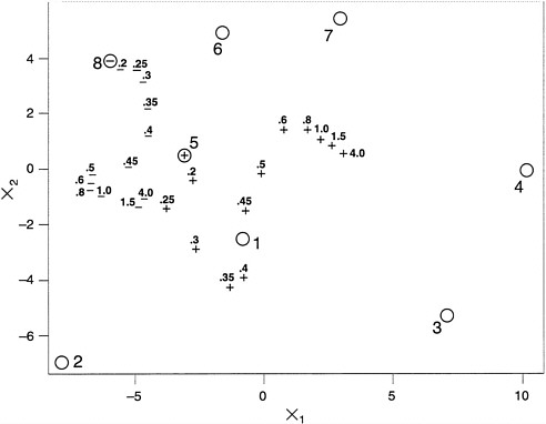
FIGURE C-1 Optimal test environments as a function of b. NOTE: For a discussion of b and of the axes and for definitions, see text.

calculated the information about the jth environment z_j. In practice, one might have to spend more assets or money on one test than another and, in that case, one could use a (further) weighted sum that would take into account how many assets were used in testing at each point x_i.

Given that two equally weighted test points will be selected, the maximin approach suggested here is to select the two test points that maximize the minimum information provided for each of the eight listed environments z₁, ..., z₈. That is, the information about z_j is cumulated over the test points and divided by the corresponding weight w_j at z_j. The overall weight w_j incorporates the frequency of occurrence and the strategic importance of the jth environment.

One potentially serious problem with this multidimensional scaling approach is that it assumes one can carry out an experiment in an environment corresponding to any point in the reduced 2-dimensional space. In reality, much of this space may not be available for testing. (For an obvious example, there are no simultaneously very hot and very cold environments.) It may therefore be difficult to construct an environment that would be mapped into a given point in the 2-dimensional space. Or there may be too many different real environments that would correspond to the same point in the 2-dimensional space.

TABLE C-4 shows the impact of changing the parameter b. When b is small, the effect of distance is slight, and it is important to make sure that the vital or highly weighted points get maximum information. Thus, the optimal design puts the two x values at the two most highly weighted environments.

When b is large, information diminishes greatly with distance from the testing point. In this case, it is necessary to move the x values to some compromise positions that provide at least some minimal information for estimating the performance in less important environments.

The impact of the choice of b is also evident in Figure C-1. Here, the position of one optimal experiment is indicated by a “+” and the second by a “−”. The environments with the highest weights, w_j, from Table C-3 are 5 and 8. For very small values of b, all environments are comparable; therefore, the two highest-weighted environments are the logical positions at which to test. This result is indicated by a “+” in the circle labeled 5 and a “−” in the circle labeled 8. As b is increased, the environments become less comparable, and the algorithm correctly selects experimental environments that are compromises of all eight environments of interest. Environments 5 and 8 are still favored, but the optimal points are now true compromises of all eight points in this 2-dimensional space. For the largest value of b, the “+” experiment is a compromise of environments 7, 4, and 3, and the “−” experiment is a compromise of environments 8, 6, 5, 1, and 2.

While this behavior may seem sensible, it depends heavily on buying into the criterion proposed. Both the exponential decline and the maximin aspects should be questioned and alternatives considered. The present formulation also ignores the possibility of replacing the single-valued information function I(x,z) by a higher-dimensional measure such as an information matrix. At the example's current level of simplicity, it seems premature to consider this latter extension.

Undoubtedly, as these alternatives and other approaches are examined, modifications of these ideas will be suggested, and useful approaches will become clear. However, because the performance of a particular statistical method may depend greatly on the structure of the individual problem, it will be essential to apply these methods to various real problems in defense testing in order to gauge their true utility.