
A Viscous Flow Simulation of Flow About the 1/40-Scale Model of the U.S. Airship Akron at Incidence Angle
C.-I. Yang (David Taylor Model Basin, USA)
ABSTRACT
A three-dimensional incompressible Navier-Stokes code based on an artifical compressibility, implicitupwind-relaxation, flux-splitting algorithm is employed to simulate the flow about a 1/40-scale model of the U.S. airship “Akron” at several incidence angles. The distributions of transverse forces along the hull and the integrated moments about the center of buoyancy are computed and comparisons with the measurements are made.
INTRODUCTION
Purely for mathematical interest, the inviscid flow about a body of revolution has long since been formulated and studied in detail. Practically, because of the predominant viscous effect near the boundary, the related flow pattern is much more complicated, especially if the body is at an incidence with respect to the flow direction. The wake of the body becomes turbulent, and various types of cross flow separation take place. The basic hull form of a modern submersible is typically a body of revolution. While maneuvering at high speed, the hull may be subject to severe hydrodynamic forces. Under certain conditions, the moment of the forces about the center of buoyancy of the body may cause instability. In order to achieve a higher envelope of maneuverability and controllability, the designers of the modern submersible have practical interest in predicting the hydrodynamic response for any given planned movement. Such interest can best be served by parallel efforts in enlarging the data base from controlled laboratory environments and developing accurate computational schemes.
Extensive experiments were carried out by various research parties, some of the representive results were reported in references (1–3). More recently, computational efforts based on newly developed numerical schemes derived from the Reynolds Averaged Navier-Stokes (RANS) formulation offer encouraging predictions (4–8).
This report present a study of the accuracy and feasibility of predicting forces and moment on a body of revolution hull form at incidence with a RANS technique. The data obtained from wind tunnel tests of a 1/40-scale model of the U.S. airship “Akron” are used for the purpose of comparison.
DESCRIPTON OF EXPERIMENT
A series of tests was made on a 1/40-scale model of the U.S. Airship “Akron” at the propeller research wind tunnel, Langley Memorial Aeronautical Laboratory (currently, NASA Langley Research Center) in 1932 (9–11). The purpose of the test was to determine the drag, lift, and pitching moments of the bare hull and the hull equipped with fins.
This particular experiment is attractive to us in some aspects: (1) the hull form is very similar to the modern high performance submersible, (2) the Reynolds number is relatively high due to the large size of the model, and (3) the data are relevent to our study; included are the distributions of the transverse forces along the hull and the moments of the forces about the center of buoyancy.
The model is of hollow wooden construction having 36 sides over the fore part of the hull, fairing into 24 sides near the stern. The length of the hull is 5.98 m.(19.62 ft.), the maximun diameter 1.01 m. (3.32 ft), the fineness ratio 5.9, the
volume 3.27m3 (115.61ft3). Four hundred pressure orifices, distributed among 26 stations, were placed along one side of the hull. The orifices were connected inside the hull to two photographic-recording multiple manometers. Each manometer consisted of 200 glass tubes placed about the periphery of a drum, a long incandescent light bulb for making the exposures was placed at the center of the drum.
Tests were conducted at several different wind speeds. The maximun speed was 44.70 m/s (100 miles per hour). The corresponding Reynolds number is about 17 million based on the length of the hull. This value is about 1/34 of the full scale ship at a speed of 37.54 m/s (84 miles per hour). The transition from laminar to turbulent flow occured at a local Reynolds number of 814000 based on the axial distance between the nose and the transition point (10). At a wind speed of 44.70 m/s (100 miles per hour), the transition point is about 0.25 m.(10 inches) from nose.
The maximum departure of the observed wind tunnel velocity from a mean value was about ±0.6 percent. The deflection of the support wire, that is the downstream movement of the model, observed at the maximum velocity of the tunnel with the hull at 0º pitch was approximately 1.5×10⁻³ m. (0.06 inch). The sources of error and the precision of measurements are discussed in detail in references 9–11.
NUMERICAL APPROXIMATION
The three-dimensional incompressible RANS equations based on primitive variables are formulated in a boundary-fitted curvilinear coordinate system and solved with an artifical compressibility concept (12). The basic operations of converting the set of differential equations to a system of difference equations may be divided into: spatial differencing and time differencing. The procedure can be described as follows.
Spatial Differencing
The three-dimensional differential operator is first split into three independent one-dimensional operators. The spatial differencing of the inviscid flux in each of these one-dimensional operators is then constructed by an upwind flux-differencing scheme based on Roe's approximate Riemann solver approach (13). In each computational cell the differential operator is linearized around an average state such that the flux difference between two adjacent cells satisfies certain conservative properties. As a result, the flux at an interface can be expressed in terms of the direction of the travelling waves. Harten's high-resolution total variation dimishing (TVD) technique (14,15) is then applied to enhance the accuracy of the solution to a higher order in the region where its variation is relatively smooth. The undesirable spurious numerical ocillations associated with high order approximations are suppressed by appling a TVD limiter. The viscous flux is centrally differenced with second-order accuracy. The overall discretization is obtained by summing up all the independent discretizations of the flux derivatives in each dimension.
Time Differencing
Since only the steady-state solutions are of interest, a first-order accurate Euler-implicit time differencing scheme is used. The application of the scheme avoids a overly restrictive time-step size when highly refined grids are used to resolve viscous effects. In addition, a spatially variable time step is used to accelerate convergence.
The governing differential equations are then reduced to a system of difference equations in “delta form”. In each time step, the corrections to the variables, instead of the variables themselves, are solved. The right hand side of the system is defined as residual. It is the explicit part of the system and has four components, one for each variable. As the solutions advance to their steady-state values through time stepping, the corrections and residuals approach zero.
The system is solved iteratively with a hybrid technique which uses approximate factorization in cross planes in combination with a planar Gauss-seidel relaxation in the third direction. The process is highly vectorizable. Presently, the L2 norm of the residual is used as a measurement of convergence of the iteration process.
As a result of upwind-differencing, the coefficient matrix of the system becomes diagonal dominant. In addition, the necessity of adding and tuning of a numerical dissipation term for stability reasons, as in some schemes with central differencing, is alleviated.
BOUNDARY CONDITION
The computational domain defined by a C-O grid extends from two body lengths upstream of the nose to two body lengths downstream of the tail in the longitudinal direction, and two body lengths from the body axis in the radial direction. On the body surface, the no-slip condition
is imposed and the normal gradient of the pressure is assumed to vanish. Free stream conditions are specified along the outer boundaries except for the outflow boundary, where the values are computed by using extrapolation. Since the flow field is symmetric with respect to the longitudinal plane of symmetry, only the flow field over half of the body is computed. Reflective conditions are then applied on the plane of symmetry. The values of the characteristic variables along the wake line are obtained by first extrapolating from interior points along each radial grid line and then taking the circumferential average. The normal distance between the body surface and the nearest grid line is 1.0×10⁻⁵ of the body length; the corresponding y+ is about 4. Computations are first performed on a grid with a 79×81×83 distribution in radial, circumferential and streamwise directions respectively. To determine the effect of gridding on the prediction of lift and cross flow separation, a grid with 79×111×83 distribution is used for a repeat computation. In both cases the circumferential spacing of radial lines is uniformly distributed, The angles between adjacent radial lines are 2.22º and 1.62º respectively.
TURBULENCE MODEL
The algebraic Balwin-Lomax turbulence model was used by Degani and Schiff (16) in computing the turbulent flows around axisymmetric bodies with crossflow separation. In order to predict multiple secondary crossflow separations at high incidence angle, modification was made such that the turbulence length scale of the outer region is determined by the viscous vorticity imbedded in the boundary layer and not the inviscid vorticity shed from the separation line. The modified model has been successfully used in several occasions to compute the turbulent flows over bodies of revolution at an incidence angle (7,16,17). The details of the modification, implementation and the physical justication can be found in Reference 16.
The behavior of the turbulent boundary layer near the stern region of an axisymmetric body has been studied extensively by Huang et al. (19). It was found that as the boundary layer thickens rapidly over the stern region, the turbulence intensity is reduced and becomes more uniformly distributed. The measured mixing length of the thick axisymmetric stern boundary layer was found to be proportional to the square root of the area of the turbulent annulus between the body surface and the edge of the boundary layer. This simple similarity hypothesis for the mixing length improved the prediction of the mean velocity distribution in the entire stern boundary layer.
Based on the above observation and results indicated in Reference 7, it is decided that algebraic Baldwin-Lomax turbulance model with Degani-Schiff's correction and Huang's modification is appropriate for present simuation.
RESULTS
The experimental data reported in References 9, 11 are massive and extensive. Our present interests are limited to the distributions of transverse forces along the bare hull and the pitching moments about the center of buoyancy of the hull at several given incidence angles. The data were presented in terms of the dynamic pressure (denoted by q) of the air stream and were corrected for the difference between the local static pressure in the stream and the reference pressure. The correction consisted simply of substracting from the pressure at any section of the model the static pressure of the air stream, measured in the absence of the model, at the corresponding point along the axis of the model. The correction reduced the pressure at the stagnation point at the nose of the hull, with the model at 0º pitch, to a value equal to the dynamic pressure q. Here, the dynamic pressure q is defined as: ![]() , where ρ is the density of the air and V∞ is the air stream velocity. Tests were conducted with the air stream at several different dynamic pressures. The highest value was 1, 225.73 Pa (25.6lb/ft2), the equivalent Reynolds number is about 17 millions based on body length. Based on this condition, the numerical simulations were carried out.
, where ρ is the density of the air and V∞ is the air stream velocity. Tests were conducted with the air stream at several different dynamic pressures. The highest value was 1, 225.73 Pa (25.6lb/ft2), the equivalent Reynolds number is about 17 millions based on body length. Based on this condition, the numerical simulations were carried out.
Predictions with the potential-based Munk and Upson equations of the transverse force at 15º of pitch were shown in Reference 11. Both predictions deviated substantially from the measurements near the stern region. The disagreements are not a surprise, since the distribution of force along the hull is strongly influenced by the surface flow separations. An engineering rational flow model based on a discrete vortex cloud method greatly enhanced the prediction (20). The improvement was attributed to a separation line model that defines the body vortex feeding sheets along the body surface. Flow visualizaton indicated that the separation patterns along a smooth surface can be quite complicated. Any further improvement in prediction at current stage may require a turbulent viscous flow approach. The
present numerical simulation assesses the feasibility and accuracy of RANS's predictions.
The profile and wire-framed perspective view of the hull are shown in Figure 1. Pressure distributions along the hull at 0º of pitch are shown in Figure 2, where the pressure is normalized with the dynamic pressure q and the distance from the nose is normalized with the hull length L. The experimental values were obtained from averaging the circumferential measurements at each of the axial locations where the pressure orifices were placed. The viscous flow solution was obtained from a computation on a 79×81×83 grid. At the mid-section of the hull, there are 28 grid points located inside the boundary layer. The CFL number used in the computation is 10. The L2 norm of the residual and the lift coefficient during the course of the iteration are shown in Figure 3. The lift force is nomalized with q(vol)2/3, where vol is the volume of the hull. The potential flow solution was obtained from a surface panel method VSAERO (21). At zero incidence, experimental data indicate that there exist a small amount of sectional transverse force along the hull at the bow and after portions of the hull. It was assumed that the air flow was not strictly axial or that the model was not exactly symmetrical.
The transverse forces along the hull at several incidence angles are shown in Figure 4. Notice that the integration of the areas underneath the curves gives the total normal forces acting on the hull. The experiment data are obtained from Table V in Reference 11. The computational results are obtained from solutions based on two grids with different densities in circumferential direction. At a given incidence, the difference between the two computational results is insignificant. Noticeable differences between experimental and computational results can be found in the stern region. The predicted and measured total transverse forces on the hull, normalized with q(vol)2/3, are shown in Figure 5 and the values are given in Table 1. The discrepancy is more perceptible at higher incidence. It was reported (11), that at high-speed, high-pitch-angle condition, the model was observed to be quite unsteady.
The axial location of the center of bouyancy of the hull is 2.77 m. (9.10 ft.) from the nose. The pitching moment about the center has two parts: (1) moment (M1) of the transverse force and (2) moment (M2) of the longitudinal force. The experiment value M1 was obtained by taking the moment of the area of the transverse force curves in figure 4 about the center of buoyancy by means of a mechanical integrator. To obtain M2, curves with transverse force at each axial location plotted against the corresponding cross-sectional area, were constructed. M2 values were then obtained by integrating the areas under the curves. The contribution of the longitudinal forces to the total moment is about 4%, and it is opposite in direction to that due to the transverse force. Lift and moment coefficients are shown in Figure 6. The Lift is normalized with q(vol)2/3, and the moment is normalized with q(vol). The values are tabulated in Tables 2 and 3 respectively. The computed values of M1 and M2 are listed in parenthesis.
In general, the measurements and the predictions are in good agreement, Noticeable differences occur only at higher incidence.
Computations have been carried out both on CRAY-YMP and CONVEX-3080 machines. Estimated CPU times are about 40μ sec per grid per iteration on CRAY-YMP and 200μ sec per grid per iteration on CONVEX-3080 in the vector mode.
CONCLUSIONS
Numerical simulations of flow about a 1/40-scale model of U.S. Airship “Akron” were carried out with RANS formulation. The effort is an attempt to predict the hydrodynamic force acting upon a body of revolution type hull form at incidence. Good and encouraging results are obtained. Further enhencement in accuracy and computational efficiency requires a improved turbulence model and a multigrid type approach. Data bases obtained with modern techniques under controlled environments are needed for validation of numerical schemes.
ACKNOWLEDGEMENT
This work was sponsored by Program Element 62323N at David Taylor Model Basin. Computing resources on a CRAY-YMP are provided by the NASA Ames Research Center under the NAS Program. The U.S. Navy Hydrodynamics/Hydroacoustics Technology Center provided computational support on a CONVEX-3080 and various work stations.
REFERENCES
1. Ramaprian, B.R., Patel, V.C., and Choi, D.H., “Mean-flow Measurements in the Three-dimensional Boundary Layer over a
Body of Revolution at Incidence,” Journal of FluidMechanics, Vol.103, 1981, pp.479–504.
2. Intermann, G.A., “Experimental Investigation of the location and Mechanism of Local Flow Separation on a 3-Caliber Tangent Ogive Cylinder at Moderate Angles of Attack,” M.S. Thesis, Universith of Florida, Gainesville, FL. 1986
3. Kim, S.E., and Patel, V.C., “Separation on a Spheroid at Incidence: Turbulent Flow,” The Second Osaka International Colloquium on Viscous Fluid Dynamics in Ship and Ocean Technology, September 27–30, 1991, Osaka.
4. Vatsa, V.N., Thomas, J.L., and Wedan, B.W., “Navier-Stokes Computations of Prolate at Angle of Attack,” AIAA Journal, Vol. 26, NO.11. 1989, pp.986–993.
5. Degani. D., Schiff, L.B., and Levy, Y., “Numerical Prediction of Subsonic Turbulent Flow over Slender Bodies at High Incidence,” AIAA Journal, Vol.29, No.12, 1991, pp.2054– 2061.
6. Hartwich, P.M., and Hall, R.M., “Navier-Stokes Solution for Vortical Flow over a Tangent-Ogive Cylinder, ” AIAA Journal, Vol.28, No.7, 1990, pp.1171–1179.
7. Sung, C-H., Griffin, M.J., Tsai, J.F., and Huang, T.T., “Incompressible Flow Computation of Force and Moments on Bodies of Revolution at Incidence,” AIAA-93–0787, 31st Aerospace Science Meeting and Exhibit, Jan. 11–14, 1993, Reno, NV.
8. Meir, H.V., and Cebeci, T., “Flow Characteristic of a body of Revolution at Incidence,” 3rd Symposium on Numerical and Physical Aspects of Aerodynamic Flows, Long Beach, California, 1985
9. Freeman, H.B., “Force Measurement on a 1/40-Scale Model of the U.S. Airship “Akron”,” T.R. No.432, NACA, 1932.
10. Freeman, H.B., “Measurements of Flow in the Biundary Layer of a 1/40-Scale Model of the U.S. Airship “Akron”,” T.R. No.430, NACA, 1932.
11. Freeman, H.B., “Pressure-Distribution Measurements on the Hull and Fins of a 1/40-Scale Model of the U.S. Airship “Akron”,” T.R. no.443, NACA, 1933
12. Chorin, A., “A Numerical Method for Solving Incompressible Viscous Flow Problems, ” Journal of Computational Physics, Vol.2, No.1, August, 1967, pp.12–26.
13. Roe, P.L., “Approximate Riemann Solvers, Parameter Vectors, and Difference Schemes, ” Journal of Computational Physics, Vol.43, No.2, 1981, pp.357–372.
14. Harten, A., “High Resolution Scheme for Hyperbolic Conservation Laws,” Journal of Computational Physics, Vol.49, No.3, 1983, pp.357–393.
15. Yee, H.C., Warming, R.F., and Harten, A., “Implicit Total Variation Diminishing (TVD) Schemes for Steady-State Calculations,” Journal of Computational Physics, No.57, 1985, pp.327–360.
16. Degani, D., and Schiff, L.B., “Computation of Turbulent Supersonic Flows around Pointed Bodies Having Crossflow Separation,” Journal of Computational Physics, Vol.66, No.1, 1986, pp.173–196
17. Vatsa, V.N., “viscous Flow Solutions for Slender Bodies of Revolution at Incidence, ” Computers Fluids, Vol.20, No.30, 1991, pp.313,320
18. Gee, K., Cummings, R.M., and Schiff, L.B., “Turbulence Model Effects on Separated Flow about a Prolate Spheroid, ” AIAA Journal, Vol.30, No.3, 1992, pp.655–664
19. Huang, T.T., Santelli, N., and Bolt, G., “Stern Boundary Layer Flow on Axisymmetric Bodies,” 12th Symposium on Naval Hydrodynamics, Washington D.C., June 1978.
20. Mendenhall, M.R., and Perkins, S., “Prediction of the Unsteady Hydrodynamic Characteristics of Submersible Vehicles,” The Proceedings, 4th International onference on Numerical Ship Hydrodynamics, Washington D.C., Sept. 24–27 1985.
21. Maskew, B., “Prediction of Subsonic Aerodynamic Characteristics—A Case for low-order Panel Methods,” AIAA-81–0252, AIAA 19th Aerospace Sciences Meeting, January, 1981.

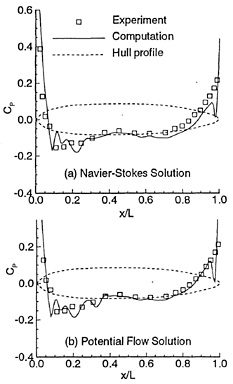


Figure 6. Lift and moment coefficients
Table 1. Transverse Force Coefficients.
|
Incidence Angle (degrees) |
Experiment |
Computation |
|
|
Grid # 1 |
Grid # 2 |
||
|
3 |
0.0127 |
0.0114 |
0.0110 |
|
6 |
0.0300 |
0.0294 |
0.0297 |
|
9 |
0.0541 |
0.0536 |
0.0515 |
|
12 |
0.0845 |
0.0883 |
0.0895 |
|
15 |
0.1246 |
0.1343 |
0.1330 |
|
18 |
0.1690 |
0.1939 |
0.1956 |
|
Grid # 1 : 79×81×83 Grid # 2 : 79×111×83 |
|||
Table 2. Lift Coefficients.
|
Incidence Angle (degrees) |
Experiment |
Computation |
|
|
Grid # 1 |
Grid # 2 |
||
|
3 |
0.011 |
0.011 |
0.011 |
|
6 |
0.029 |
0.028 |
0.027 |
|
9 |
0.054 |
0.051 |
0.047 |
|
12 |
0.080 |
0.083 |
0.081 |
|
15 |
0.115 |
0.125 |
0.121 |
|
18 |
0.155 |
0.178 |
0.173 |
|
Grid # 1 : 79×81×83 Grid #2 : 79×111×83 |
|||
Table 3. Pitching Moment Coefficients.
|
Incidence Angle (degrees) |
Experiment |
Computation |
|
|
Grid # 1 |
Grid #2 |
||
|
3 |
0.078 |
0.081 (0.084, −0.003) |
0.081 (0.084, −0.003) |
|
6 |
0.150 |
0.156 (0.162, −0.006) |
0.153 (0.159, −0.006) |
|
9 |
0.212 |
0.222 (0.230, −0.008) |
0.222 (0.230. −0.008) |
|
12 |
0.260 |
0.276 (0.286. −0.010) |
0.271 (0.282, −0.010) |
|
15 |
0.307 |
0.316 (0.327, −0.011) |
0.310 (0.322, −0.012) |
|
18 |
0.348 |
0.339 (0.352. −0.013) |
0.347 (0.360, −0.013) |
|
Grid # 1 : 79×81×83 Grid # 2 : 79×111×83 |
|||
The Prediction of Nominal Wake Using CFD
A.J.Musker, S.J.Watson, P.W.Bull, and C.Richardsen
(Defence Research Agency, England)
ABSTRACT
A study of the effect of systematically applying different CFD methods and associated parameters is described for the case of the HSVA tanker. Attention is focussed on the propeller plane and the nominal wake in particular. The viscous solutions are compared with an inviscid solution and with experiment data in an attempt to discover how well current codes perform in terms of practical predictions of propeller inflow. It has been found that the flow in the outer region of the propeller disc can be defined with reasonable accuracy. However, the methods fail to describe the flow at the half-radius position.
NOMENCLATURE
|
Cμ |
constant of proportionality for the eddy viscosity |
|
k |
turbulence kinetic energy |
|
Lpp |
length between forward perpendiculars |
|
r |
radial length from propeller axis |
|
RD |
radius of grid domain |
|
R |
propeller radius |
|
Ut |
tangential fluid velocity |
|
Ux |
axial fluid velocity at propeller plane |
|
U∞ |
free-stream fluid velocity |
|
w |
Taylor wake fraction |
|
w1 |
average circumferential wake fraction |
|
w2 |
volumetric mean wake fraction |
|
x |
longitudinal distance from forward perpendicular |
|
|
turbulence diffusion rate |
|
θ |
angle between propeller radius and horizontal radius |
INTRODUCTION
In recent years a great deal of effort has been spent on developing numerical techniques to solve the Navier-Stokes equations of fluid motion. For practical reasons, these fundamental equations need to be ‘Reynolds-averaged' and, in so doing, some error is incurred in the modelling. Additional errors are incurred in the choice of the closing turbulence model and also in the various numerical processes invoked to solve the equations. These processes include the discretisation scheme, the grid resolution, cell disposition and quality, choice of solution algorithm and choice of convergence criteria.
This paper describes some recent experiences in predicting the nominal wake of a surface ship using advanced computational fluid dynamics procedures. The paper is the third in a series on CFD validation originating from the CFD Section at the Defence Research Agency, Haslar [1, 2]; these studies concentrate on the issue of numerical verification. A validated CFD capability should enable the designer to make use of the computed velocity field in the propeller plane to aid in the design of a suitable propeller. Not only would this enable more candidate hulls to be assessed and placed in rank order of performance, but it might also permit significant reductions in design costs to be gained.
Whilst the ship hydrodynamics community must continue to support and encourage the development of new methods to aid in ship design, it should, every once in a while, stop to examine the capability that currently exists and then match that capability to the requirements of the naval designer. In this way, any serious shortfall in
capability will be identified and this should determine the level of effort required to improve the methods. In the authors' opinion, such a ‘definition of capability' for stern flows is still lacking in the ship hydrodynamics literature; the most recent qualitative attempt was made by Larsson, Patel and Dyne [3].
In their study, an international workshop was organised to establish how accurately the velocity field could be predicted in the stern region of a model tanker which had been tested in a wind-tunnel at the University of Hamburg. The workshop attracted 19 teams from many nations and provided an excellent forum for establishing the world-wide capability. It also highlighted the extreme difficulty facing the CFD teams with respect to the sensitivity of their predictions to the choice of the various numerical methods and parameters associated with the conduct of their calculations.
An additional but related difficulty facing the organisers concerned the lack of any control relating to these parameters—particularly the grid size. Nearly all the participants ‘broke the rules' imposed by the organisers and this made the task of comparing the predictions associated with the various methods very difficult. Half of the teams managed to produce results which resembled the experiment measurements, and one or two performed rather better than this but were still regarded by the workshop participants as insufficiently accurate.
This paper concentrates on the first of the two test-cases under investigation in the above workshop, namely, the problem of predicting the nominal wake (by which is meant the propeller is absent) for the HSVA hull at a Reynolds number of 5×10⁶. The investigation was initiated in response to a growing awareness within the International Towing Tank Conference (ITTC) community that in recent years too little attention has been paid to issues relating to the validation of CFD.
The authors use computational fluid dynamics (CFD) methods to calculate the fluid velocity in the propeller disc to deduce the Taylor wake fraction and the associated radial and circumferential distributions of wake. This is compared with experiment data in a systematic manner and under reasonably well controlled numerical conditions. The k-∊ turbulence model is used throughout, although subtle differences exist between the codes concerning the wall treatment.
Control over the investigation is imposed by ensuring that the datum conditions for the computer runs, for example the number of computational cells for the two types of grid, structured and unstructured, remain approximately the same.
Clearly, there is considerable scope for improving this approach to numerical verification through additional effort and expense (perhaps using finer grids, or more sophisticated turbulence models). However, statements concerning accuracy can still be made, albeit pragmatic ones, based on a typical set of default conditions derived on the basis of wide experience in using these methods. It is hoped that the investigation will help the community to judge the present capability of available CFD codes, as applied to the practical prediction of nominal wake.
SOLUTION METHODS
Overview
The solution methods which are appropriate for solving the RANS (Reynolds-Averaged Navier-Stokes) equations fall into three broad categories: finite difference, finite volume and finite element methods. Each method has certain apparent advantages depending on the complexity and nature of the application, although it has to be said that practically no research has been undertaken aimed at ranking the performance of the methods for typical naval problems. Indeed, this is one of the aims of the Haslar team. In this study, five methods were tried, although two of them were similar in terms of the detailed solution technique employed. For the purpose of the present paper, we shall refer to the different methods by a simple numbering system.
Finite difference methods rely on replacing individual partial derivatives by algebraic equivalents which are local to a particular location, or cell, within the fluid domain. The finite analytic method also falls into this category except that the difference equations are related to locally analytic forms of the master equations (Method 1).
Finite volume methods use integral formulations of the RANS equations applied to a large number of control volumes constructed using
the computational grid. Such methods offer the advantage of examining fluxes through a well-defined volume and as such allow local continuity to be satisfied more easily (Method 2).
Finite element methods rely on expressing the local variation of each primitive variable within a cell (or element) by a shape function. The equations are re-cast in terms of the various shape functions chosen and a set of residuals is formed. These are weighted on the basis of the coefficients used in the shape function and the equations are solved for zero weighted residuals; this is the basis of the so-called Galerkin method. In principle this method ought to be the most accurate, but it can be memory intensive and therefore expensive to run (Method 3).
All the methods require the generation of a computational grid of cells. This can be performed either algebraically, using trans-finite interpolation, or numerically, using a set of Poisson equations relating the physical space to a convenient logical computational space (in which grid lines are straight and parallel and orthogonal in the coordinate directions). In the latter procedure, the governing master equations are transformed into a curvilinear, body-fitted coordinate system which maps across to the computational grid.
A severe restriction imposed by many CFD methods is that they are designed to work on only ‘structured' grids in which cells are arranged in contiguous order in a logical space. For appended bodies, the structured approach can only be used by assembling blocks of structured grids together such that the total grid containing all the blocks fills the physical domain. The flow code then has to be organised so that information at block boundary faces can be easily communicated to adjacent block faces with the minimum of distortion. This is the basis of the multi-block approach (Method 4).
For the finite volume and finite element codes, however, the grid can be totally unstructured and the equations need not be transformed to a curvilinear coordinate system. In principle, this should lead to greater flexibility in the disposition and clustering of cells for regions within the domain where high gradients of velocity occur, and may allow greater flexibility with regard to building grids around complex geometries. Of course, this extra flexibility is gained at the considerable expense of more computer time and memory, since the move away from a contiguous ordering of cells imposes a need to store the cell connectivity in the form of additional look-up tables.
The different methods used in the present study will now be outlined.
Method 1
This method was developed by Patel, Chen and Ju at the Iowa Institute of Hydraulic Research and has been partially validated by them in a separate report [4]. The method, now embodied in the RANSSTERN computer code, employs the three-dimensional RANS equations for steady, incompressible flow. The Reynolds stresses are related to the corresponding mean rate of strain using the eddy viscosity concept. The eddy viscosity is calculated from the standard two-equation k-∊ model with convective transport equations for the turbulence kinetic energy and dissipation rate. All of the equations are written in dimensionless form, using a partial transformation, where only the independent coordinate variables are transformed from the physical domain to a logical computational domain. The coordinate transformation is defined using a set of Poisson equations with the computational coordinates as the dependent variables and the Cartesian coordinates as the independent variables. A cylindrical polar coordinate system is used as the basic physical coordinate system, with velocity components in the axial, radial and circumferential directions.
The momentum and turbulence equations are recast using transformations into the computational domain and rearranged into general convective transport equations with suitable source terms. These equations are discretised using the finite-analytic (FA) method which reduces them to a set of fully implicit equations, in space and time, which can be solved by a tridiagonal matrix algorithm. The continuity equation, however, is solved using a modified version of the SIMPLER algorithm [5], which produces equations for pressure correction terms and pressure using a staggered grid. These equations are also discretised using the finite analytic method and solved using a tridiagonal matrix algorithm.
The complete solution is obtained firstly by solving the momentum, pressure correction and turbulence equations in planes marching downstream and then by solving the pressure equations in planes
marching upstream. This ensures that the elliptic nature of the equations is maintained and improves the convergence rate of the solution. An iterative procedure is used to link the pressure field to the velocity and turbulence fields. Although the calculation is steady-state, the method uses a time-marching technique in which a time step corresponds to one outer iteration, the steady-state solution being obtained after sufficient time steps. The convergence rate is controlled using suitable values of the time step and successive under-relaxation parameters.
The wall function on the ship surface uses a two point formulation and the effects of pressure gradients on the flow in the wall region are taken into account using a generalised law of the wall due to Chen and Patel [6].
Method 2
This method was developed by Lonsdale and Webster [7] of the United Kingdom Atomic Energy Authority and is now embodied in the ASTEC computer code. The method represents a major extension of ideas and techniques for two-dimensional flows reported by Baliga and Patankar [8]. Features held in common with method 1 include the application of the three dimensional RANS equations subject to the assumptions of steady, incompressible flow, and the eddy viscosity concept calculated from the convective transport equations for k and ∈. The constants used for the k-∈ model in both methods were identical. Method 2 uses a standard logarithmic wall function (without the pressure gradient correction incorporated in method 1).
The underlying approach, however, is very different from, and conceptually simpler than, method 1. The most obvious difference relates to the solution of the equations in the physical space rather than a transformed computational space. As a consequence, method 2 uses very different discretisation procedures.
Integral forms of the RANS equations are solved numerically by applying them to control volumes which surround each node within the domain. The velocity components are defined at each node and the pressure is defined at each cell centre. A cell is here restricted to an eight-noded hexahedron. The control volumes are constructed around the cell nodes by firstly joining the centroids of each cell face to the centroid of the cell. In this manner each hexahedral cell is divided into eight smaller hexahedra—each one of which includes a cell node. The smaller hexahedra associated with neighbouring cells surrounding a given node are then joined to define a control volume.
A purely geometrical approach is used to quantify the various terms appearing in the integral equations. For example, the divergence theorem of Gauss is invoked to convert the pressure gradient term to a surface integral of pressure. The latter is easily evaluated by summing the contributions from individual faces of a given control surface, subject to the assumption that the pressure for a face is given by the pressure for the element containing the face. Indeed it is a feature of the method that any flux associated with a control surface face is calculated using only nodal information belonging to the element containing the face.
The diffusion term is treated in a similar manner to the pressure gradient term. In this case, the fluid velocity gradients are defined for each control surface by linear interpolation of the current velocity components applied to sets of tetrahedra constructed within each element. The advection term is calculated using a skew-upwind hybrid differencing scheme. This scheme allows various blends of central and upwind differencing to provide the usual compromise between accuracy and stability. In addition, however, the scheme also allows upwind discretisation in the local stream-wise direction in an attempt to reduce the amount of false numerical diffusion associated with highly skewed flows. This facility is provided by a set of weighting factors applied to the nodes of the upwind element face. These factors are set according to the point of intersection of an element streamline (emanating from a given downstream node) and the upwind face of the corresponding element.
The resulting discretised equations are solved using a segregated approach. The momentum equations are solved using a Gauss-Seidel solver; for the continuity equation, the SIMPLE algorithm is applied and the equation is solved using a preconditioned conjugate gradient method. A modification of the Rhie and Chow [9] procedure is used to improve the stability of the pressure correction scheme applied at each element. Although a pseudo-unsteady approach is also used in this method, the time step can be chosen to be very large.
Method 3
The suite of computer programs, FIDAP (written by Fluid Dynamics International [10]) can be used to simulate a variety of flow conditions. FIDAP is a Petrov-Galerkin based finite element method for computational meshes which can be either structured or unstructured.
Tri-linear basis functions were used for velocity, except in those cells abutting hull surfaces; piece-wise constants were used for pressure. The discretized equations of motion are solved in a segregated manner with the equations for each variable being solved in turn using the preconditioned conjugate gradient technique. Note that streamline up-winding was used to enhance the stability of the discretized transport equations.
Pressure correction is employed to ensure mass conservation. In the modelling of the effect of the hull shear layer, FIDAP uses a wall function approach with the turbulent kinetic energy providing the velocity scale for the wall functions. For mesh cells abutting the hull, FIDAP uses a single velocity profile, the so-called Reichardt law, to modify the velocity basis function in the direction normal to the wall. Similarly, the eddy viscosity is modified using a van Driest damping factor normal to the wall.
Method 4
The DRA code, RANSBLOCK, is a suite of computer programs which is based on the multi-block technique for solving the RANS equations for complex geometries. The multi-block technique decomposes the flow domain into a number of blocks and uses a communication strategy to transfer global conservation of mass and momentum. RANSBLOCK uses a transformation from body-fitted coordinates to logical computational coordinates for each block in the domain. The coefficients for the discretisation scheme are evaluated using the finite analytic approach, in an identical manner to RANSSTERN. RANSBLOCK uses a structured block scheme and is fully three-dimensional, which gives considerable flexibility for generating body fitted meshes, unlike RANSSTERN which is limited to parallel x-planes.
As in RANSSTERN, the Chen and Patel [6] wall function is used; this includes a correction term for the prevailing pressure gradient.
The overall solution strategy involves the calculation of velocity, mass source and turbulence fields for each block using the momentum, pressure correction and turbulence equations. These results are communicated to adjoining blocks using interpolation schemes for each block. The pressure field is then calculated for each block. The complete process is repeated a number of times until the continuity equation is satisfied to within a given tolerance.
Method 5
This method provides a non-lifting potential flow solution to the problem. The method, embodied in the DRA code known as BRAC, is a panel method and was devised by the first author for predicting non-linear wave resistance [11]. However, in this instance, the code was run at negligible Froude number in order to provide a basis for assessing the improvement to be gained by adopting a fully viscous method using a RANS code.
CONDUCT OF INVESTIGATION
Run Attributes
The aim of the investigation was to record changes in the numerical solution arising from changes in the details associated with implementing a particular method or problem specification. Such details will be referred to as ‘attributes'. The particular attributes chosen for the investigation were:
-
Turbulence Model
The k-ε model was used with three different values of Cμ (the constant of proportionality relating the eddy viscosity to the computed ratio k2/ε). The values used were Cμ, 1/2Cμ and 2Cμ. Alternatively, the modified k-ε model due to Chen and Kim [12] could be chosen instead.
-
Grid
Six different grids were generated. Three of these were plane-by-plane structured grids, as required by Method 1; the resolutions were 21,168 cells (datum standard), 64,584 cells (medium resolution) and 390,818 cells (high resolution). Two unstructured grids were included, although
-
they were unstructured only in transverse planes; both represented attempts to concentrate cells around regions of high curvature and near the propulsor disc. The ‘unstructured 1' grid comprised 21,756 hexahedral cells, whilst the ‘unstructured 2' grid comprised 21,854 cells which were mostly hexahedral but included some wedge cells near the stern. Finally, a 3D surface-by-surface (as opposed to plane-by-plane) structured grid, was also included.
The grids filled a cylindrical domain whose nominal dimensions were x/Lpp=0.3 to x/Lpp= 2.5, and RD/Lpp=0.75, where Lpp is the length of the ship, x is the distance measured from the bow, and RD is the radial distance from the longitudinal axis.
-
Alignment of model in computational domain
The longitudinal axis of the model could be chosen to be either parallel to the onset flow or to make a small angle (in pitch and/or yaw) to the onset flow (in such cases, the removal of symmetry planes doubled, or quadrupled, the number of computational cells). This attribute was included in the investigation to determine how sensitive the flow-field in the experiment might have been to small errors in model alignment.
-
Inclusion of supporting wire
In the wind-tunnel experiment [13], the stern region of the model was supported by a thin wire on each side. The wire was connected to the keel of the hull at x/L pp=0.81 (the authors are indebted to Dr J Kux for providing this information) and formed an angle of 45º to the horizontal. In the calculations, this wire could be either ignored or modelled (albeit crudely by invoking a no-slip boundary condition at nodes nearest to the wire).
Strategy
The verification process can be conveniently described in terms of an imaginary machine. Associated with this machine is a set of five switches, each of which can change the setting of an attribute in accordance with the options available, as described above.
The datum set of attributes was:
-
turbulence: standard k-∈
-
plane-by-plane structured grid (23,750) (as used in ref [2])
-
model axis parallel to onset flow
-
wire ignored
This datum set of attributes corresponds to all the switches being set at ‘zero', as shown in Table 1.
In order to exercise proper control over the investigation, no more than two switch settings were allowed to have non-zero values for a given run. For example, if the model was inclined (see the ‘alignment attribute in Table 1), with the alignment switch set to 1, 2 or 3, then all other switches would have been set to zero (the datum setting).
It was not possible to test all the methods with all the switch positions; however, all the methods were applied to the datum case (all switch settings set to zero). The actual runs performed are indicated in Tables 2 to 5. Each ‘yes' entry is a single run, with all other attribute switches set to zero.
DATA REDUCTION
Attention was focussed exclusively on the velocity field within a prescribed area in the propeller plane (defined to be a plane through the propeller position and perpendicular to the longitudinal axis). This area extended to two propeller diameters below the hull and to 1.5 propeller diameters outwards from the centre-plane. Within this region, each data set was linearly interpolated onto a uniform reticle for ease of comparison.
The following parameters were calculated for each computer run:
-
the Taylor wake fraction, w, at the radius of the propeller disc, and at half the radius:
w(r,θ)=Ux(r,θ)/U∞
-
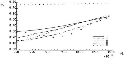
average circumferential Taylor wake fraction, w1:

-
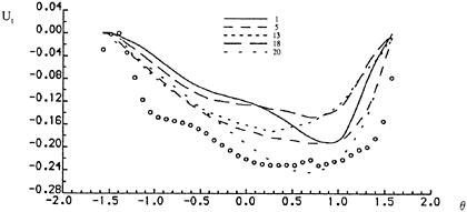
the circumferential variation in the tangential velocity component, Ut, at the radius of the propeller disc, and at half the radius.
-
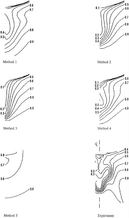
contours of constant axial velocity.
-
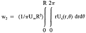
volumetric mean wake fraction, w2:
All integrations were performed using Simpson's rule after demonstrating that the arithmetic was sensibly independent of the chosen step-length.
DISCUSSION OF RESULTS
A project of this nature generates a huge amount of data; specifically, 120 graphs were produced for analysis, together with the 20 values of mean volumetric wake fraction. Accordingly, this section will concentrate on the salient features and trends observed in the results. For convenience, all the runs are listed in Table 6 so that the reader can associate a particular run with the method and switch setting(s) identified in the Tables 1–5; note that only runs 10 and 12 had more than one non-zero switch setting.
In all the subsequent plots, the experiment data are indicated by open circular symbols, and the CFD data by spline curves derived from the raw calculations. Plots involving circumferential variations are displayed according to the convention that θ increases from −π/2 at the bottom of the (imaginary) propeller disc to +π/2 at the top (nearest the double body symmetry plane). Plots involving radial variations (w1) increase from zero (centre of disc) to the outer radius of the disc. The predicted values for the volumetric mean wake fraction, w2, are shown in the right-hand column of Table 6. For all the predictions shown in the following figures, the run number is indicated so that the reader can recover the particular switch settings from Tables 1–6.
We shall start with the effect of changing the flow solution method for the datum cases, where all the switches were set to zero. The results are shown in Figures 1 to 6.
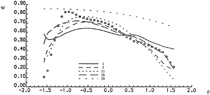
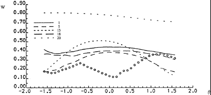
With the possible exception of Method 1 (run 1), which strays significantly from the experiment data, the Taylor wake fraction at the edge of the propeller disc (Figure 1) is predicted reasonably accurately. The viscous effects are clearly captured, as can be seen by comparing all the predictions with Method 5 (run 20)—the inviscid model. At half the radius, however, all the methods fail to describe the shape of the experiment curve. The circumferential variation of the wake fraction is shown in Figure 3. Again, the shape of the experiment curve is not depicted in any of the predictions, although in quantitative terms all the viscous codes have succeeded in reducing w1 to its correct value at the edge of the disc. At half the radius, errors are typically 30%.
Figure 4 shows the tangential velocity at the radius of the disc. Interestingly, the inviscid code (run 20) performs better than all the viscous codes — a fortunate consequence of the location of the circumference of the disc with respect to the measured cross-flow; the inviscid code does not generate vortical features and this result should be regarded as coincidental.
The situation is very different at half the disc radius (Figure 5), where the longitudinal vorticity is high. Clearly the flow is dominated by viscous effects, and these are reflected in the predictions only in the sense of a general trend towards correctly increasing Ut compared with inviscid theory. The axial velocity contours are compared with experiment, using all the methods, in Figure 6. Note that the so-called ‘hook' [3] in the experiment curve is missing from all the predictions.
Method 3 was used to investigate the sensitivity of the predictions to changes in the attitude of the model with respect to the inflow. These ‘perturbations' were introduced in an attempt, to discover whether a small alignment error in the wind-tunnel might help to explain the differences observed within the core of the vortical flow. The only positive conclusion that can be drawn from this
exercise is that the discrepancy diminishes slightly when the double-body hull is pitched by an angle of plus two degrees (Figure 7). However, the oscillating character of the experiment data is still not reproduced.
The effect of changing the turbulence representation in Method 2 is shown in Figure 8 for the case of Ut at the disc radius. Significant improvements are found when Cμ is halved (run 6) and when the Chen and Kim model is used (run 8). This suggests that either k is over-predicted, or that ![]() is under-predicted, in the standard k-∊ model. However, the predictions of Ut at the edge of the disc are no better than those of Method 5 (the inviscid method), so it is possible that all the viscous solutions suffer from too much numerical diffusivity compared with the eddy diffusivity computed from the standard 2-equation model.
is under-predicted, in the standard k-∊ model. However, the predictions of Ut at the edge of the disc are no better than those of Method 5 (the inviscid method), so it is possible that all the viscous solutions suffer from too much numerical diffusivity compared with the eddy diffusivity computed from the standard 2-equation model.
Method 1 was used to assess the effect of the cell density on the solution; some results for the wake fraction at the edge of the disc are shown in Figure 9. Although the calculated values of w at the bottom of the disc ( −π/2) are too high, there is clearly an improvement to be gained by adopting a denser grid (runs 3 and 4).
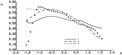
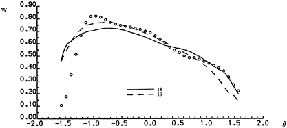
The multi-block code (Method 4) was used to study the effect of switching from a standard (vertical) plane-by-plane (PBP) grid (run 18) to a more versatile (non-vertical) surface-by-surface (SBS) grid (run 19); the results are shown in Figure 10. Here, the peak at approximately—1 radian is more clearly described by the SBS grid compared with the PBP grid. However, the SBS grid tends to under-predict slightly at the top of the disc.
Figure 11 shows the effect of changing from a structured grid (run 5) to an unstructured grid (run 11). A clear improvement is noticed, similar to the observation made above regarding the effect of halving Cμ, suggesting that the unstructured grid is less diffusive than the structured grid.
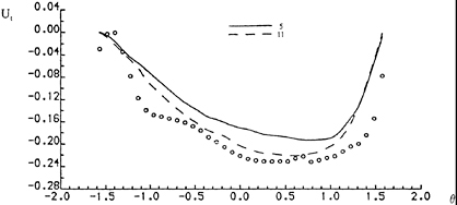
We now come to the effect of incorporating the support wire. This was investigated by simply applying a no-slip boundary condition at nodes nearest to the wire but without any attempt to cluster cells around it. Consequently, some features of the flow in the propeller plane are adversely affected by this crude modelling. This is exemplified in Figure 12, where the momentum deficit is greatly increased (run 9) compared with the datum case without the wire (run 5). However, at the half-radius position (Figure 13), there is a considerable improvement in the top-most region of the disc compared with the datum runs shown in Figure 2. Similarly, although the absolute values of the circumferentially-averaged wake fraction, w1 (Figure 14), are too low compared with the datum run (run 5), the prediction with the wire (run 9) does exhibit the point of inflection in the region of r/L=0.005. The comparisons for Ut at the edge of the disc, and at the half-radius position, are shown in Figures 15 and 16. Note that there was little improvement, in terms of general trends, associated with the use of the Chen and Kim turbulence model or the unstructured grid (runs 10 and 12—not shown).
Attention must now be drawn to a somewhat surprising outcome of this investigation. Figure 17 shows a comparison between run 5 (the datum run for Method 2) and run 9 (with the wire included) for the case of the constant axial velocity contours. It can be seen that there is a very pronounce ‘hook' which appears in the experiment and is reproduced in run 9; this Figure should be compared with Figure 6, which displays the datum runs for all the methods. It must be emphasised that the only change to the datum run was the application of a set of no-slip conditions to those nodes closest to the wire; the grid and all other features remained the same.
Finally, the volumetric mean wake fraction, w2, is listed in Table 6 for all the runs performed. The mean of all the runs (excluding the inviscid method) is 0.39, compared with the experiment value of 0.37 as calculated using the same procedures as those employed in the analysis of the CFD data.
CONCLUSIONS
A numerical verification study into the effects of the choice of solution algorithm, turbulence model, grid, model alignment and model support arrangements has been conducted for the case of the HSVA tanker at a Reynolds number of 5×10⁶. The propeller was absent throughout the investigation. The following conclusions are drawn:
-
RANS methods provide a good overall description of the flow near the edge of the propeller disc. In this region, the predictions are
-
reasonably independent of the choice of solution method adopted.
-
The predictions break down in the region within the disc; specifically, the predictions were generally poor at the half-radius position. In this region, changing the choice of solution method brought about changes in the solution which were comparable in magnitude with the changes associated with the choice of computational grid.
-
Changes to the standard k-∊ turbulence model, including drastic changes to the constant of proportionality for the eddy viscosity, produced relatively little change in the predicted wake. The observed changes were considerably smaller than those associated with the choice of other attributes.
-
Changes arising from the use of different grids resulted in significant changes to the solution. Switching from a plane-by-plane grid to a 3D surface-by-surface grid, from a coarse to a fine grid, and from a structured grid to an unstructured grid, led to improvements in the predictions at the edge of the disc.
-
Simulations of the effect of poor model alignment in the wind-tunnel have demonstrated that a 2º error in yaw or pitch creates a greater change to the nominal wake than any change brought about by the choice of any of the numerical attributes associated with the generation of a solution for a naked hull.
-
By appending the hull to a support wire attached to the keel at x/Lpp=0.81, as was done in the experiment, and applying a no-slip boundary condition to nodes closest to the wire, the solution was observed to change radically. No attempt was made to wrap a stretched grid around the wire, as this would have disrupted the control of the experiment (since the cell count would have increased dramatically). Although the crude approach adopted led to worse quantitative predictions of the nominal wake, it dramatically improved the qualitative prediction of the axial velocity contours. Specifically, the so-called ‘hook ' was captured in the solution.
Further work is planned to confirm what is now a mere suspicion; namely, that the failure to describe the measured axial velocity contours, using RANS methods, may be due to the actual experiment conditions having been neglected.
REFERENCES
1. Musker, A.J., “Stability and Accuracy of a Non-Linear Model for the Wave Resistance Problem,” Proceedings of the 5th International Conference on Numerical Ship Hydrodynamics, Hiroshima, September 1989.
2. Musker, A.J., Atkins, D.J., Watson, S.J. and Bull, P.W., “A Comparison of Two Navier-Stokes Methods Applied to the Stern Region of the HSVA Tanker,” Proceedings of the 2nd International Colloquium on Viscous Fluid Dynamics in Ship and Ocean Technology , Japan, September, 1991.
3. Larsson, L. and Patel, V.C., “Proceedings of the 1990 SSPA-CTH-IIHR Workshop on Ship Viscous Flow,” Goteborg, September 1990.
4. Patel, V.C., Chen, H.C. and Ju, S., “Ship Stern and Wake Flows: Solutions of the Fully-Elliptic Reynolds-Averaged Navier-Stokes Equations and Comparisons with Experiments,” IIHR Report No 323, April 1988.
5. Patankar, S.V., “Numerical Heat Transfer and Fluid Flow,” McGraw-Hill, New York, 1980.
6. Chen, H.C. and Patel, V.C., “Calculation of Trailing Edge, Stern and Wake Flows by a Time-Marching Solution of the Partially Parabolic Equations”, IIHR Report No 285, 1985.
7. Lonsdale, R.D. and Webster, R., “The Application of Finite Volume Methods for Modelling Three-Dimensional Incompressible Flow on an Unstructured Mesh,” Proceedings of the 6th International Conference on Numerical Methods in Laminar and Turbulent Flow, Swansea, England, July 1989.
8. Baliga, B.R. and Patankar, S.V., “A Control Volume—Finite Element Method for Two Dimensional Fluid Flow and Heat Transfer, ” Numerical Heat Transfer, 6, pp 245–261, 1983.
9. Rhie, C.M. and Chow, W.L., “Numerical Study of the Turbulent Flow Past an Airfoil with Trailing Edge Separation,” AIAA Journal 21, No 11, 1983.
10. FIDAP User Manual Volume 1—Theory. Fluid Dynamics International Inc., Evanston, IL, USA. April 1991.
11. Musker, A.J., “Panel Method for Predicting Ship Wave Resistance,” Proceedings of the 17th Symposium on Naval Hydrodynamics, The Hague, 1989.
12. Chen, Y.-S and Kim, S.-W, “Computation of Turbulent Flows Using an Extended k-∈ Turbulence Closure Model,” NASA Report CR-179204, October 1987.
13. Wieghardt, K and Kux, J.Nomineller Nachstrom auf Grund von Windkanalkversuchen, Jahrbuch der Schiffbautechnischen Gesellschaft (STG), Springer Verlag , pp 303–318, 1980.
Table 1—Switch/Attribute Matrix
|
switch # |
turbulence |
grid |
alignment |
wire |
|
0 (datum) |
k-∈ |
standard structured |
perfect |
ignored |
|
1 |
1/2Cμ |
unstructured 1 |
±20 yaw |
included |
|
2 |
2Cμ |
unstructured 2 |
+20 pitch |
- |
|
3 |
Chen and Kim |
medium structured |
−20 pitch |
- |
|
4 |
- |
high structured |
- |
- |
|
5 |
- |
3D |
- |
- |
Table 2—Verification Runs for Method 1
|
switch # |
turbulence |
grid |
alignment |
wire |
|
1 |
no |
no |
no |
no |
|
2 |
no |
no |
no |
- |
|
3 |
yes |
yes |
no |
- |
|
4 |
- |
yes |
- |
- |
|
5 |
- |
no |
- |
- |
Table 3—Verification Runs for Method 2
|
switch # |
turbulence |
grid |
alignment |
wire |
|
1 |
yes |
yes |
no |
yes |
|
2 |
yes |
no |
no |
- |
|
3 |
yes |
no |
no |
- |
|
4 |
- |
no |
- |
- |
|
5 |
- |
no |
- |
- |
Table 4—Verification Runs for Method 3
|
switch # |
turbulence |
grid |
alignment |
wire |
|
1 |
no |
no |
yes |
no |
|
2 |
no |
yes |
yes |
- |
|
3 |
no |
no |
yes |
- |
|
4 |
- |
no |
- |
- |
|
5 |
- |
no |
- |
- |
Table 5—Verification Runs for Method 4
|
switch # |
turbulence |
grid |
alignment |
wire |
|
1 |
no |
no |
no |
no |
|
2 |
no |
no |
no |
- |
|
3 |
no |
no |
no |
- |
|
4 |
- |
no |
- |
- |
|
5 |
- |
yes |
- |
- |
Table 6—Description of Run Numbers
|
Run # |
Method |
Switch Setting(s) |
w2 |
|
1 |
1 |
datum #0 |
0.46 |
|
2 |
1 |
turbulence #3 |
0.48 |
|
3 |
1 |
grid #3 |
0.46 |
|
4 |
1 |
grid #4 |
0.50 |
|
5 |
2 |
datum #0 |
0.38 |
|
6 |
2 |
turbulence #1 |
0.40 |
|
7 |
2 |
turbulence #2 |
0.43 |
|
8 |
2 |
turbulence #3 |
0.41 |
|
9 |
2 |
wire #1 |
0.21 |
|
10 |
2 |
wire #1, turbulence #3 |
0.23 |
|
11 |
2 |
grid #1 |
0.41 |
|
12 |
2 |
wire #1, grid #1 |
0.33 |
|
13 |
3 |
datum #0 |
0.44 |
|
14 |
3 |
alignment #1 |
0.33/0.51 |
|
15 |
3 |
alignment #2 |
0.31 |
|
16 |
3 |
alignment #3 |
0.21 |
|
17 |
3 |
grid #2 |
0.40 |
|
18 |
4 |
datum #0 |
0.45 |
|
19 |
4 |
grid #5 |
0.46 |
|
20 |
5 |
see text |
0.78 |


DISCUSSION
by Professor D.L.Whitfield, Mississippi State University.
To simulate the influence of the support wire on the experimental measurements you stated you adjusted the computed velocity. Another way the authors might consider simulating the support wire numerically would be to use the drag force of the wire (which can be estimated rather accurately) as a body force in the equations used for the numerical simulation. This approach is simple to use and doesn't require extensive grid modifications other than, perhaps, some aligning of the grid in the region of the support wire.
Author's Reply
To clarify any confusion, note that we simulated the presence of the support wire by specifying values of velocity as boundary conditions at grid points lying near to the actual physical position of the wire throughout its length and not by modifying computed velocities.
As to representing the wire as a body force in the equations of motion, we agree that this approach would be worthy of further investigation. However, although Professor Whitfield's comments about the modifications to the mesh are valid, we believe that the mesh would have been optimal had it been designed to accommodate the presence of the wire at the outset, so as to avoid numerical complications and ambiguities.
DISCUSSION
by Dr. J.Kux, Institut für Schiffbau, Universitat Hamburg
The authors are to be complimented for this thorough study of wake prediction by applying different CFD methods to the case of the HSVA tanker.
As originator of the experimental data about the flow field of the so called HSVA1 test case, I feel that some remarks concerning the wake of this hull form should be appended here. The authors claim, though at present as “a mere suspicion,” that their failure in reproducing the experimental findings “may be due to the actual experiment conditions having been neglected” and here the main point alluded to, is the suspension wire with its wake interfering with the double model wake in the region scanned. Since this is—if really the wake is basically altered due to the wire—a severe objection against this data set to be used as test case, the matter should be thoroughly ventilated. At the moment a new run with the HSVA1 double model in the wind tunnel with changed support wire location is not feasible. Therefore it is appropriate to review evidence against the cited suspicion. This has to include a critical discussion of the arguments presented, as well as a search for cases with similar wake details (hoods) from model investigations where no supporting wires were present, a summary of our scrutiny of the details of the wire wake and of computational evidence, that the hood may well be obtained with no need to simulate wires, but merely by slightly increasing the sophistication of the turbulence model use.
The basic problem when comparing two flows, here one measured with one computed, is the choice and weighting of the criteria on which to base figures of merit. There are several quantities such as scalar (i.e., pressure), vector (i.e., mean velocity, wall shear-stress) and even tensorial (i.e., Reynolds-stress) fields which should enter the comparison. Here a singular feature, the famous “hook,” a detail of the isoline pattern of the longitudinal component of the mean velocity field, has been overemphasized and shown to be reproducible by a computational intervention, without the vortical pattern of the transverse components of the mean velocity, which has to go with it, being depicted for this computational attempt. The feature “hook” has been achieved by a questionable technique of an artificial non-slip boundary condition on some nodes close to the wire, at locations which are not disclosed in the paper. Further details of the fields are not shown: Does the wall shear-stress distribution, or the distribution of k, the kinetic energy of turbulence, obtained with this wire simulation, compare qualitatively better or worse to the experimental findings than without wire simulation? It should not be overlooked, that, as stated by the authors, quantitatively this crude intervention led to a deterioration of predictions.
Now if we look for evidence of “hooks” in wake velocity patterns from towed models, (no
suspension wires, no struts) we readily hit upon such: merely a few will be cited. Tanaka (1988, Figure 23, Page 345) shows such a wake pattern for three geosims of a tanker, Ogiwara in its contribution relating to one of the new test cases to be proposed by the Resistance and Flow Committee of the ITTC, the “Ryuko Maru,” presents such an isoline pattern (Figure 10, Section C), and for the other test case, the so called Hamburg Test Case, towed in the HSVA [Betram et al., 1992], the vestige of a “hook” appears in the nominal wake (Abb. 5–30) (as in the experimental findings from the double model of this hull in the wind tunnel at the IfS), which develops into a enormous “hook” under the action of the propeller at certain propeller-loadings (Abb. 5–38). Finally, also in this conference we have seen a similar pattern [Suzuki et al. 1993] (Figure 6), for the nominal wake developing behind the so called propeller open boat in an experiment designed to investigate the interaction of the propeller slipstream with the rudder.
The velocity field for the HSVA1 test case was thoroughly investigated by us several years ago, when we were first faced with the details disclosed by the experiment. One step was the computation of the vorticity field, the curl of the vector field of the mean velocity. In the wake of the wire, vorticity values were derived, but this vorticity was aligned—as to be expected—with the wire direction and no longitudinal component of the vorticity appeared. In the area of interest, there is, of course, a superposition of this vorticity to the one from the flow field. Nevertheless, specifically in the core domain of the longitudinal vortex, and therefore at the “hook,” this original vorticity is strongly aligned with the velocity vector, i.e., we have high helicity there (while over most of the region, vorticity and velocity tend to be almost at right angles), an alignment process initiated by the three-dimensional thick boundary layer, where the vorticity vector, due to the cross flow, leaves its circumferential direction (originally in a transverse plane as in a nearly two dimensional boundary layer) initiating the formation of the characteristic longitudinal vortex. The wire-induced vorticity, being aligned neither with the vortex core vorticity nor with the original boundary layer vorticity, it does not seem likely that the wire wake induces a basically different flow pattern from that which would develop in the absence of the wire.
Different authors managed to reproduce the “hook,” in the near past, in their computational studies. At the Gothenburg workshop [Larsson et al., 1991], Zhu & Miyata (Figure 8), at the Osaka Colloquium 1991, Sung et al [Sung et al, 1991] (Figure 20), and at this conference Zhu et al., [Zhu et al 1993] (Figure 12c), using hybrid turbulence model and Deng et al., [Deng et al., 1993] (Figure 18), with an unconventional localized change of the eddy viscosity otherwise obtained by the standard k-Ɛ-model. In the last mentioned contribution, a quite reasonable resulting wall shear-stress directional pattern is presented too. Remarkably in this paper, these results were obtained by reducing the value of the (scalar) eddy viscosity in the core of the longitudinal vortex thus enhancing the inhomogeneity of the simulated turbulence considerably in contrast to the model prediction. The simple change of the eddy viscosity by a factor, as in the paper here discussed, could not be expected to render any dramatic influence, since the scalar viscosity is differentiated (multiplied to the symmetrisized stress tensor) in the momentum equations. This shows that the nowadays popular use of a scalar eddy viscosity, common to all the components of the Reynolds tensor, is an oversimplification. Any anisotropy deviation from that of the stress tensor is suppressed. Even when we accept a scalar eddy viscosity, in the k-Ɛ-model, k is a scalar by definition, while Ɛ is the trace of what originally entered the scene as a tensor, the dissipation in the transport equations of the Reynolds stress tensor components, a tensor with an anisotropy that is sacrificed both, to keep the model simple and since no sound empirical indications are available to model it.
1. Bertram, V., Chao, K.Y., Lammers, G., and Laudan, J., “Entwicklung und Verifikation Numerischer Verfahren zur Antriebsleistungsprognose, Phase 2,” Report No. 1579, The Hamburg Ship Model Basin, HSVA, 1992
2. Deng, G.B., Queutey, P., and Visonneau, M., “Navier-Stokes Computation of Ship Stern Flows: A Detailed Comparative Study of Turbulence Models and Discretization Schemes,” Proceedings of the Sixth
International Conference on Numerical Ship Hydrodynamics, Iowa City, Iowa, 1993
3. Larsson, L., Patel, V.C., and Dyne, G., Editors: “Ship Viscous Flow,” Proceedings of the 1990 SSPA-CTH-IIHR Workshop, Gothenburg, Research Report No. 2, Flowtech International AB, 1991
4. Sung, C.H., Griffin, M.J., Smith, W.E., and Huang, T.T., “Computation of Viscous Ship Stern and Wake Flow,” The Second Osaka International Colloquium on Viscous Fluid Dynamics in Ship and Ocean Technology, Osaka, 1991, Proceedings
5. Suzuki, H., Toda, Y., and Suzuki, T., “Computation of Viscous Flow Around a Rudder Behind a Propeller—Laminar Flow Around a Flat Plate Rudder in Propeller Slipstream,” Sixth International Conference on Numerical Ship Hydrodynamics, Iowa City, Iowa, 1993, Proceedings
6. Tanaka, I., “Three-Dimensional Ship Boundary Layer and Wake,” Advances in Applied Mechanics, Vol. 26, 1988, Pages 311–359
7. Zhu, M., Yoshida, O., Miyata, H., and Aoki, K., “Verification of the Viscous Flow-Field Simulation for Practical Hull Forms by a Finite-Volume Method,” Proceedings of the Sixth International Conference on Numerical Ship Hydrody-namics, Iowa City, Iowa, 1993
Author's Reply
Dr. Kux is right to point out that the “hook” for the HSVA1 experiment data is by no means unique, but it should not be forgotten that the other examples cited were not, in my opinion, subjected to the same degree of rigorous scrutiny as was exercised by the Hamburg term. Experiments involving supporting struts for models show that junction vortices formed where a strut joins a model can be extremely persistent and can interfere with measurements well downstream. Of course, as Dr. Kux rightly points out, in the HSVA1 case the axis of vorticity is parallel to the wire downstream and away from the model. But at the junction with the hull, the vorticity associated with the developing shear layer will be deflected as the fluid streams past the wire. Consequently, I believe it is possible that the wire represents a source of interference to the measured nominal wake and that one should not ignore its presence on the grounds, for example, that its diameter is small or that other precedents may have been set for models towed in a tank (without support wires).
On the other hand, the work presented by Deng et al at this Conference has opened up the possibility that the hook is indeed a feature of the flow-field and not, as we have suggested, an aberration caused by the wire. It is always possible, of course, that the wire itself was responsible, in a fortuitous way, for numerically attenuating the eddy diffusivity within the bilge vortex further downstream! This needs to be confirmed and is now being investigated at Haslar.
I am unaware of any hook having been predicted unequivocally by other teams. It was my understanding that the 1990 Gothenburg Workshop prediction by Zhu and Miyata was later withdrawn after an error had been detected in the computer code (reported at the 1991 Osaka Colloquium). The numerical results for the SR196 hull series presented by Zhu. Yoshida and Miyata at this Conference do not, in my opinion, show clear signs of any hook—although it is prominent in the experiment. The results of Sung et al at the 1991 Osaka Colloquium show a very weak hook (compared with the experiment) but only for their medium grid data; the two other grids, one with eight times as many cells and the other with eight times fewer cells, show no trace whatsoever of a hook.
On a more general note, one very useful outcome of the recent ITTC effort to place CFD validation very firmly on the ship hydrodynamics agenda, has been the realization that systematic studies can indeed point to possible explanations of observed phenomena. In the case of the notorious “hook”, we now have two pointers as to its possible cause and I hope very much that other teams will now join the effort to resolve this elusive riddle. While our computers may converge towards a sound numerical solution, we must step back and converge towards a sound physical solution. Whether this will involve a closer look at the precise details of the experiment, or—now more likely—a closer look at how our turbulence models can be made to deal more adequately with vortical regions, remains to be seen.
Numerical Prediction of Viscous Flows Around Two Bodies by a Vortex Method
Y.M.Scolan and O.Faltinsen
(University of Trondheim, Norway)
ABSTRACT
Viscous incompressible flows around two identical circular cylinders are simulated by using a Mixed Euler-Lagrange Method. The Vortex-In-Cell Method is combined with the Operator Splitting Technique and a Random Method. The vorticity field is represented by a set of discrete vortices which are transported in the fluid by solving the Navier Stokes equations in the subcritical flow regime. The interaction of two bodies is studied through the combination of the Conformal Mapping Technique and the Green's Theorem. The obtained results show that the physical phenomena can in general be satisfactory predicted for two cylinders in either side-by-side or tandem arrangements. Comparisons are made with experimental data for oscillating and steady ambient flows. The presented method may handle two arbitrary cross-sectional shapes. The model may also be extented to super-critical flow regimes.
NOMENCLATURE
|
Ci |
contour of cylinder Nºi |
|
d |
distance between the centers of the two circular cylinders |
|
a |
radius of one circular cylinder |
|
ρ |
mass density of the fluid |
|
U |
amplitude of the ambient harmonic oscillatory flow velocity or the ambient steady flow velocity |
|
L |
characteristic length of one body (L=2a) |
|
T |
period of the oscillatory ambient flow velocity |
|
ν |
kinematic viscosity coefficient |
|
fo |
frequency of vortex shedding |
|
Δt |
time step |
|
Re |
Reynolds number |
|
KC |
Keulegan-Carpenter number |
|
β |
Stokes parameter |
|
St |
Strouhal number |
|
CD |
drag coefficient |
|
CL |
lift coefficient |
|
CM |
mass coefficient |
THEORETICAL MODEL
The numerical scheme is a combination of the Vortex-In-Cell Method (VIC) as it has originally been introduced by (1) and the Operator Splitting Technique used by (2) to simulate the transport of vorticity. For the two past decades the VIC Method has been continuously improved. Therefore the theory will not be detailed in the present paper but the main features of the basic method are recalled. For more details one can refer to (3) and also to the significant contributions by (4,5,6,7).
The Vortex-In-Cell Method and the Random Method
Since planar flows are considered here, the equations are formulated in terms of the vorticity ω and the stream function ψ. In the Poisson equation
Δψ=−ω (1)
the right hand side (ω) is represented by a set of Lagrangian particles (or vortices) with positions (xl,yl) carrying each a certain amount of circulation (Гl) constant in time:
(2)
Here δ is the Dirac delta function. The vorticity field is distributed on the cell-nodes of an Eulerian mesh which covers a limited computational domain. This is done by the Area Weighting Scheme as it has been originally proposed by (1). In the present method the Poisson equation will always be solved in an annular domain. The Elliptic Solver is decomposed in a Finite Difference Method for the resolution in the radial direction and a Fast Fourier Transform for the azimuthal direction.
The generation of vortices takes place on the body contours in order to respect the no-slip condition. The local tangential component of the velocity provides the circulation of the new set of discrete vortices. The vorticity is transported in the fluid by solving the Navier Stokes equation in the laminar flow regime. The Operator Splitting Technique (OST) is used. The convection step consists of moving the vortices with their local velocity without change of their circulation. The convection motion is performed by a second order Runge-Kutta integration scheme. The diffusion step consists of superimposing a random walk to the the position of the vortices. The random numbers are distributed according to a normal law with a zero mean value and a standard deviation ![]() , where Δt is the time step and ν is the kinematic viscosity coefficient.
, where Δt is the time step and ν is the kinematic viscosity coefficient.
The whole process described above is repeated in time. That leads to a continuous production of vorticity. The Kelvin Theorem (zero total circulation around a curve surrounding the generated vorticity from the bodies) must be respected since no vorticity exists at the initial instant.
Due to the way that the effect of diffusion is simulated, it should be noted that all the local variables (vorticity, stream function, velocity…) and therefore the forces themselves may be affected by a small random component: this grows with ![]()
As the number of vortices increases in time, it is necessary to reduce the number of vortices if one wants to perform long simulations in time. This can be achieved in two ways. One concerns the treatment of vortices which enter the body due to the random walk. The technique which is used here is similar to the one presented in (6). The vortices which enter the body contour, are coalesced at the nearest nodes of the contour mesh. Then new vortices are re-injected into the fluid at a certain radial distance. This distance is chosen in the same sequence of random numbers as for the diffusion process. This technique allows one to keep constant the rate of circulation per time step, and leads to a considerable decrease of the number of vortices present in the fluid. This optimization is particularly important for ambient oscillatory flows when many vortices remain close to the body contour due to the reversal of the flow. However this advantage still holds, but to a lesser extent, for steady incident current. In this case the coalescence of vortices far away from the bodies is the best way of reducing the number of vortices. In practice the coalescence occurs in a special region which overlaps a part of the wake far away from the bodies. As soon as this zone contains vortices enough, the coalescence happens. More details will be given later in the text in connection with the numerical modelling of the physical problem.
Extension to Multi-body Configurations
The modelling of viscous flows around multiple cylinders has been investigated for the past decade. The validation has been essentially done by comparisons with experimental data for two identical circular cylinders of radius a spaced with a distance d between the centers.
The already existing techniques consist of using several levels of overlapping meshes in the physical plane (see (6)). The successive solutions from the coarsest mesh to the finest ones provide the boundary conditions of all intermediate Boundary Value Problems (BVP). Results for the pressure have been compared with experiments in the turbulent flow regime. Those experiments have been performed in a wind tunnel (see (9) and (10)). Numerical results for two staggered cylinders are available in (11) where comparisons are made with experimental data as well. However, if one cylinder is directly situated in the wake of the second, the Vortex-In-Cell Method applied to supercritical flow regimes has difficulties. The reason is lack of accuracy in modelling the flow in the gap. The shortest gap of two tandem cylinders computed by (11), is two diameters between the cylinder centers. More recently, one can find in (12), results by using the Vortex-In-Cell Method in combination with a Random Method. They used three levels of overlapping meshes to solve the Poisson equation. The generation of vortices is otherwise achieved through an integral equation which provides directly the circulation of the newly created discrete vortices. Besides they reported that in experiments, “some aspects of large-scale wake behaviour associated with vortex shedding
are similar at low Reynolds numbers (100– 200) and at high Reynolds numbers (greater than 104). Thus, for the tandem arrangement, they computed the drag force at a low Reynolds number Re=200 for a spacing varying from d/a=2.4 up to d/a=14.
In this paper, only moderate subcritical flows are considered. The smallest computed gap is d/a=2.5. Numerical difficulties may occur at a smaller gap. This has not been systematically investigated. However, it should be noted that the limitation on the value of the gaps, in the present numerical model, is connected to the discretization of the fluid domain in the close vicinity of each solid contour. In order to avoid several levels of overlapping meshes, the combination of a Conformal Mapping and the Green's Theorem is used. The convection of all the vortices present in the fluid at one time step requires three solutions of the Poisson equation. The first one will be obtained in a transformed plane. The Conformal Mapping transforms the physical fluid domain (limited by the boundaries of the two circles) into a simpler computational domain. Different types of transformation may be used. The main criteria for choosing adequate transformations are:
-
the conservation (through the transformation) of both the geometrical boundary and the conditions which are prescribed on them,
-
the suitability of the simplest mesh in the computational domain of the transformed plane to the physical phenomenon of interest.
This actually leads to a transformation which preserves the boundary contour as streamlines whatever the plane, and also refines the physical mesh in the gap between the two cylinders. The chosen transformation has been widely used for solving compressible flows around multi-foils. The analytical developments may be found in (13) and applications are available in (14) or (15).
The VIC Method provides a solution in the transformed plane. However this solution may not be accurate enough all over the boundary layers close to each solid boundary. Therefore additional problems should be solved for each body. The VIC Method is solved for each cylinder, in a domain (as regular as possible) surrounding the body. The outer boundary of that domain is also a circle. On this boundary a condition is established by using the Green'sTheorem. Thus, two sub-problems are successively solved in the physical plane.
Mapping of two cylinders into an annulus
The exterior domain of two arbitrary cylinders C1 and C2 may be mapped into an annular domain bounded by two concentric circular cylinders. The notations (see (16)) are described in figure (1)(a,b). The physical and transformed geometries are defined in the z-plane and the ζ-plane, respectively. The radius of cylinder Nºi is ri, in the physical plane. Later in the text, the radii will be chosen equal and denoted by a. The position of the center of cylinder Nºi is zi. The distance between the two cylinders is denoted d=|z2−z1|. The angle ![]() is the orientation of the line joining the two centers relative to the x-axis. In the transformed plane, the radius of cylinder Nºi is Ri and the position of the center of the concentric cylinders is denoted ζo. The equation of the transformation may be written:
is the orientation of the line joining the two centers relative to the x-axis. In the transformed plane, the radius of cylinder Nºi is Ri and the position of the center of the concentric cylinders is denoted ζo. The equation of the transformation may be written:
(3)
with
(4)
and
(5)
In the general case two constants are arbitrary and for simplicity one can fix: ζo=0 and mini(Ri)=1, so that the governing equation is:
(6)
with
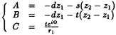
(7)
The image of physical infinity in the transformed plane is located at ζ∞=CR1.
Since a constant mesh is used in the azimuthal direction of the transformed plane, the size of the cells varies considerably from one solid contour to the other one.
The complex inverse Jacobian1 of the transformation is:
(8)
(9)
The mapping derivative ![]() has no singular point since z=−B/d is always located inside one of the two bodies. When |z| → ∞ or alternatively ζ → ζ∞, the mapping derivative behaves as
has no singular point since z=−B/d is always located inside one of the two bodies. When |z| → ∞ or alternatively ζ → ζ∞, the mapping derivative behaves as ![]() . The Jacobian itself (i.e.
. The Jacobian itself (i.e. ![]() ) is singular at infinity.
) is singular at infinity.
The relation between the two complex velocities in the z- and ζ-planes are:
(10)
From this last relation, one can show that an uniform current in the physical plane is represented in the transformed plane by a doublet located precisely at ζ=ζ∞. The complex velocity at ζ∞ behaves as:
(11)
Figures (2)(a,b) illustrate the Conformal Transformation. The arrow-plot shows the velocity pattern around two staggered cylinders in unseparated flow. The uniform current is directed horizontally from the left to the right. The starting point of each arrow is the image of the regular polar mesh nodes shown in the transformed plane. The image of the infinity and origin of the physical plane are also marked in the transformed plane. The mesh in the transformed plane has been expanded exponentially in the radial direction. This causes an approximately constant distance between mesh points along the line joining the centers of the two bodies in the physical plane.
SOLUTION OF THE BOUNDARY VALUE PROBLEM
Due to the linearity of the Poisson equation, the stream function can be decomposed into the following three components:
-
the unperturbed flow component (ψ∞) corresponding to the ambient flow without any solid contours and no vortices in the fluid,
-
the perfect fluid component (ψp) representing the perturbation of the ambient flow due to the bodies, but without any free vorticity in the fluid,
-
the vortex component (ψν) taking into account the presence of the vortices around the solid boundaries.
The perfect fluid solution (ψp) is obtained by the Boundary Integral Equation Method (BIEM). The vortex solution (ψν) is calculated from the solutions of the VIC Method in both the transformed and the physical planes.
The Perfect Fluid Solution
This solution depends only on the geometry, the direction of the unperturbed flow![]() and varies linearly with .
and varies linearly with .![]() This solution is obtained by solving the following BVP for the stream function ψp:
This solution is obtained by solving the following BVP for the stream function ψp:
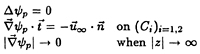
(12)
A right-handed coordinate system ![]() is defined on the body contour. The unit normal vector
is defined on the body contour. The unit normal vector ![]() points into the fluid domain and the direction of
points into the fluid domain and the direction of ![]() is anti-clock wise. The solution of equation (12) is represented by a distribution of sources and dipoles over the body contours. The resulting integral equation is solved by a Collocation Method. The singularity strengths vary linearly over each segment of discretization. Since the two cylinders are fixed in the plane, the matrix of the linear equation system does not depend on time but only on the geometry. This means that the perfect fluid solution can be calculated once and for all. The linear equation system is solved by a classical direct elimination scheme of the Gauss type. The velocity is also represented with an integral form by differentiating the basic integral equation for ψp. The total perfect fluid velocity is finally given by:
is anti-clock wise. The solution of equation (12) is represented by a distribution of sources and dipoles over the body contours. The resulting integral equation is solved by a Collocation Method. The singularity strengths vary linearly over each segment of discretization. Since the two cylinders are fixed in the plane, the matrix of the linear equation system does not depend on time but only on the geometry. This means that the perfect fluid solution can be calculated once and for all. The linear equation system is solved by a classical direct elimination scheme of the Gauss type. The velocity is also represented with an integral form by differentiating the basic integral equation for ψp. The total perfect fluid velocity is finally given by:
(13)
In practice the contours of the two unit circles are each discretized into 90 segments.
|
1 |
The Jacobian of the transformation between the physical and transformed planes (respectively z and ζ) is defined as J=dz/dζ. The proper definition of the Jacobian is the ratio of the infinitely small areas of the two planes: |dz|dζ|2. |
The convergence tests showed this discretization is fine enough to have accurate results whatever the relative position of the two cylinders is. The perfect fluid velocity is calculated in the physical plane for points that are images of the polar mesh nodes defined in the transformed plane (see figures (2)(a,b)). Thus the perfect fluid velocity at any point of the physical plane is interpolated from the values given on that mesh.
The Vortex Solution
The vortex solution gives the velocity induced by the free vortices in the fluid. The computation is divided in two main steps. A first solution is obtained in the transformed plane. This gives the convection velocity of vortices which are located beyond a certain distance from the solid boundaries. Then the Poisson equation is solved successively on two polar meshes surrounding each circular body. The latter solution gives the convection velocity of vortices close to the body contours. Figure (1)(a,b) give the notations of the different domains where a standard BVP is solved.
The BVP in the transformed plane
This BVP is posed in the annular domain defined by the polar coordinates ζ= ρeiλ and it is bounded by R2<|ζ|<R1. One must find the solution of:
(14)
where ![]() (t) are only functions of time (t). If one denotes δψν the jump of the stream function between the two bodies, then it can be calculated as the flux of velocity between the two bodies by using:
(t) are only functions of time (t). If one denotes δψν the jump of the stream function between the two bodies, then it can be calculated as the flux of velocity between the two bodies by using:
(15)
The integration is performed between the points P1 and P2 which are located on the two solid contours, respectively C1 and C2. The vector ![]() is directed from C1 to C2. The set of vectors
is directed from C1 to C2. The set of vectors ![]() is right-handed. The quantity
is right-handed. The quantity ![]() is the physical velocity induced by the vortices only in the presence of the solid contours. This velocity is obtained at a certain time instant from the solution calculated at the previous time step on the polar meshes surrounding each body.
is the physical velocity induced by the vortices only in the presence of the solid contours. This velocity is obtained at a certain time instant from the solution calculated at the previous time step on the polar meshes surrounding each body.
A particular solution of the BVP defined in equation (14) may be obtained by taking ω=0. The solution can be written:
(16)
where A(t),B(t) are two functions of time. The velocity in the transformed plane is:
(17)
which can be expressed with its complex form in the physical plane by using equation (10):
(18)
This solution represents a flow whose intensity increases in the gap but vanishes rapidly elsewhere.
The general vortex solution is calculated with the VIC Method. The problem given by equation (14) is solved with homogeneous Dirichlet conditions on the two solid boundaries. The computational domain is annular and the mesh is polar. The azimuthal step is constant and the number of segments is Nλ=27=128. This is a power of 2 in order to solve the Poisson equation by using a Fast Fourier Transformation. There are ![]() nodes in the radial direction. The mesh is refined exponentially close to the inner contour in order to have approximately a constant radial step in the gap of the physical plane.
nodes in the radial direction. The mesh is refined exponentially close to the inner contour in order to have approximately a constant radial step in the gap of the physical plane.
The sum of the particular and general vortex solution provides the velocity ![]() induced by the vortices (and only them) in the presence of the two solid contours. Finally, by adding the perfect fluid solution given by equation (13), the resulting velocity is used to convect the vortices which are located outside the outer boundary of two polar meshes surrounding each body.
induced by the vortices (and only them) in the presence of the two solid contours. Finally, by adding the perfect fluid solution given by equation (13), the resulting velocity is used to convect the vortices which are located outside the outer boundary of two polar meshes surrounding each body.
The BVPs in the physical plane
In order to represent accurately the boundary layer which is formed around each solid contour, the Poisson equation is solved in an annular domain around each body. The
inner and outer boundaries are respectively the solid contours (Cj)j=1,2 and the circles (Σj)j=1,2 of radius ![]() Σj centered at the position zi. The radii (
Σj centered at the position zi. The radii (![]() ∑j) j=1,2 are chosen so that the two outer boundaries (∑j) j=1,2 do not intersect, but they may touch in one point.
∑j) j=1,2 are chosen so that the two outer boundaries (∑j) j=1,2 do not intersect, but they may touch in one point.
The two BVPs are solved successively and separately in the physical plane. The calculation of the boundary conditions for each BVP is described in a coordinate system centered at the position zi. The cartesian and polar coordinates are denoted respectively (x,y) and (![]() ,θ) whatever the BVP since those are solved separately and in an exactly similar way.
,θ) whatever the BVP since those are solved separately and in an exactly similar way.
The interaction between the two bodies appears in the outer boundary conditions. On the boundary (Σj) one has to match the two components of the velocity. This is achieved by using the Green's second identity, which relates the following two functions:
-
the total stream function ψ,
-
a test function φ which is harmonic.
The resulting integral equation is:

(19)
where n denotes the outward normal on the contour (∂Ωe) The domain Ωe is limited by the outer boundary (∑j), the boundary of the other cylinder (Ci)i≠j and a circular control surface (∑∞) extending to infinity. The integral over the solid contour (Ci)i≠j vanishes. This follows from the Gauss Divergence Theorem, the fact that this surface is a streamline and that the normal gradient of the stream function (ψ,n) is exactly the tangential velocity. The latter must vanish on the contour due to the no-slip condition. It remains finally the contribution of the surfaces (∑j) and (∑∞) in the integral equation (19). On the surface (∑∞) the vorticity vanishes. Hence, the total stream function ψ is matched on (∑∞) with the stream function of the unperturbed flow plus the stream function of a dipole in order to take into account the presence of the bodies. The behavior of ψ and its radial gradient on the surface (∑∞) is:
(20)
(21)
The test function is otherwise calculated by using the Method of Separation of Variables. The only possible set of solutions is:
(22)
where m is a positive integer number. The function φm is singular at the origin zi, which is outside the domain Ωe.
The stream function is decomposed in a truncated Fourier Series of the polar angle (θ), i.e.

(23)
The number of modes of the Fourier development is ![]() and Nθ denotes also the number of nodes in the azimuthal direction of the polar mesh. The expressions of ψ and φ are included in the Green's identity (19):
and Nθ denotes also the number of nodes in the azimuthal direction of the polar mesh. The expressions of ψ and φ are included in the Green's identity (19):
(24)
Here δ is the Kroenecker symbol and m is an integer number of the interval ![]() The equation for the mode 0 reduces to:
The equation for the mode 0 reduces to:
(25)
The right hand side of the last equation represents exactly the amount of circulation which lies outside the surface (∑j) and therefore balances the circulation which is inside the polar mesh due to the Kelvin Theorem. In the computations one may increase the stability of the simulations by taking the average of the total circulations lying inside and outside the surface (∑j):
(26)
The development for the non-zero modes may be pursued by using equation (2). The integral term in the right hand side of equation (24) may be developed as:
(27)
The outer boundary condition is a mixed (or Fourier) condition. This condition is written for a given mode m and depends only on the radius ![]() Σj. For body Nºj, the BVP posed in the polar mesh may now be written as:
Σj. For body Nºj, the BVP posed in the polar mesh may now be written as:

(28)
where the last condition is defined by equation (24). In order to be consistent, the two first equations are Fourier tranformed. Then, the resulting BVP is classicaly solved for each mode by a Finite Difference Method. The solution ψ gives, after differentiation, the total velocity which is used to convect the vortices lying inside the two polar meshes. The non-homogeneous Dirichlet condition in the BVP defined by equation (28) does not affect the results for the velocity.
NUMERICAL PARAMETERS
Two parameters govern the physics of the problem. These are the Keulegan —Carpenter number ![]() and the Reynolds number
and the Reynolds number ![]() , where U and T are respectively the amplitude and the period of the oscillating current velocity, L is a characteristic length of the body shape. In the following applications, L denotes the diameter of one cylinder, that is to say L=2a. A third coefficient is usually introduced for the oscillating flows: the Stokes Parameter
, where U and T are respectively the amplitude and the period of the oscillating current velocity, L is a characteristic length of the body shape. In the following applications, L denotes the diameter of one cylinder, that is to say L=2a. A third coefficient is usually introduced for the oscillating flows: the Stokes Parameter ![]() . In addition, for steady flows the Strouhal number
. In addition, for steady flows the Strouhal number ![]() where fo is the frequency of the vortex shedding, will be used.
where fo is the frequency of the vortex shedding, will be used.
The force acting on each body is calculated at each time instant of a simulation. The instantaneous force F(t) follows from integration of the Cauchy Stress Tensor whose radial and tangential components correspond respectively to the effect of the pressure and the skin friction.
For steady incident flows, the drag coefficient (CD) is calculated in the direction on the ambient flow, and the lift coefficient (CL) is calculated in the transverse direction.
The force coefficients for oscillating ambient flows are partially defined by the Morison's equation which states that the force F(t) in the direction of the ambient planar flow u(t) can be written:

(29)
Here |.| denotes the absolute value. The velocity oscillates at the circular frequency of oscillation ω and behaves as u(t)= U sin(ωt). The drag coefficient CD characterizes the force in phase with the ambient fluid velocity. The mass coefficient CM is connected with the force in phase with the ambient fluid acceleration. These two main coefficients are calculated from the history of the force by Fourier averaging over one cycle. This is performed according to the following two formulas:
(30)
(31)
RESULTS AND DISCUSSIONS
Computations have been performed for two arrangements of cylinders:
-
two tandem cylinders in either oscillating or steady ambient flows,
-
two side-by-side cylinders in a steady ambient flow.
Comparisons have been made with available experimental data. The numerical parameters are given for each arrangement and type of flow.
Two Cylinders in a Tandem Arrangement and in an Oscillating Ambient Flow
The two gaps d/a=4 and d/a=8 are investigated at a Stokes parameter β= 534. Comparisons are made with two sets of experimental data: by (17) at β=534 and by (18) at Re=2.5 · 104 and d/a=3 and 5.
The time simulations are always performed over a number of cycles of oscillations (Nc) as large as possible. Nc decreases mainly with an increasing Keulegan-Carpenter number and to a lesser extent with
an increasing Reynolds number. The final force coefficient is the mean value over the total number of simulated cycles. Besides, the standard deviations, for each coefficient, are calculated over the total number of cycles of oscillations, in order to quantify how the force coefficients vary from one cycle to another cycle.
The time step has been chosen in order to have 100 time step per period up to KC= 2.5 that is to say ![]() . However, for higher KC, the time step is limited to
. However, for higher KC, the time step is limited to ![]() = 0.025.
= 0.025.
The simulations for two tandem cylinders have been performed by imposing numerical symmetry about the axis going through the centers of the two cylinders. This is necessary in order to avoid numerical difficulties with a possible orbital current generated during the reversal of the flow. As a matter of fact, a slight asymmetry of the boundary condition on the outer radius (r=r∑j)j=1,2, may induce an orbital current along the body contour. This amplifies very rapidly since the tangential velocity, calculated on the solid contour, provides the strengths of the newly created discrete vortices. Therefore the production of vortices carrying each a very large circulation, affects seriously the stability of the time simulation. The imposed symmetry can be justified up to KC≈4. However beyond that limit the use of the numerical symmetry is more questionnable. As a matter of fact, it has been observed by (19) that the wake behind one circle starts to be asymmetric in the interval ![]() .
.
The figures (3)(a,b) and (4)(a,b) show the results at respectively d/a=4 and d/a=8. The drag coefficients are identical for the two cylinders at small KC numbers. The minimum value of CD appears at KC=2.4 and KC=2 for d/a=4 and d/a=8, respectively. Then the drag coefficient increases with increasing KC-numbers to almost constant values of CD≈1.2 for d/a=4 and CD≈1.3 for d/a=8. The results show a small oscillatory behavior of CD as a function of KC for KC>6. This is most pronounced at d/a=4. The comparison with experimental data can be made in the interval ![]() . In that range the present numerical results and the experimental data by (17) do not show the same trend. Beyond KC=6, whatever the spacing, the computed drag coefficient does not increase but remains close to a constant value. However the numerical values match well with the experimental data by (18). These experimental data have been obtained at a high subcritical Reynolds number Re=2.5 · 104 while the highest Reynolds number in the present computations is Re=4272.
. In that range the present numerical results and the experimental data by (17) do not show the same trend. Beyond KC=6, whatever the spacing, the computed drag coefficient does not increase but remains close to a constant value. However the numerical values match well with the experimental data by (18). These experimental data have been obtained at a high subcritical Reynolds number Re=2.5 · 104 while the highest Reynolds number in the present computations is Re=4272.
Concerning the mass coefficient, an asymptotic limit can be calculated at KC= 0. For the two gaps d/a=4 and d/a= 8 the mass coefficient tends respectively to CM≈1.97 and CM≈2.06. These values can also be compared to theoretical results for a single circular cylinder. For example (20) obtained an asymptotic expansion for small KC-numbers of the mass coefficient as a function of the Stokes parameter (β). According to (20), CM=2.09 for β=534.
For ![]() the computed mass coefficients do not follow the decreasing trend shown by the experimental data in (17). But the present numerical data and the experimental data by (18) match well at KC≈8.
the computed mass coefficients do not follow the decreasing trend shown by the experimental data in (17). But the present numerical data and the experimental data by (18) match well at KC≈8.
Tables (1) to (4) summarize also the performed computations. The results show that the number of simulated cycles decreases as the KC-number increases. The reason is that the maximum number of discrete vortices has been reached (this is fixed to 200.000 in the computer program). In connection with the decreasing number of simulated cycles, one should note the increasing standard deviation with increasing KC-number.
Two Tandem Cylinders in a Steady Incident Flow
For the tandem arrangement in steady incident flow, (21) reported that there exists a critical spacing in the sub critical and laminar flow regimes. This critical spacing may vary in the interval d/a≈[6.8, 7.6]. Below these values, vortex shedding does not occur from the upstream cylinder but only from the downstream cylinder. Beyond this critical value, vortex shedding occurs separately from each cylinder. Results are obtained here for a spacing d/a=6 (that is to say below the critical spacing) at low Reynolds numbers ![]() . The numerical parameters of the time simulation are the following:
. The numerical parameters of the time simulation are the following:
-
the time step is
 and the simulations are performed over 1000 time steps,
 -
the radial discretization in the transformed plane is
 ,
,
-
in the physical plane the radius of the outer boundary is
 and the number of radial nodes Nr varies with the Reynolds number from Nr =21 to 60.
The coalescence of vortices takes place in a annulus domain defined by ![]() [10., 11.5] and centered at the middle of the line joining the centers of the two cylinders. A grid of 5 radial nodes and Nθ=128 azimuthal nodes covers this annulus. Only that part of the annulus which overlaps the wake is used. The coalescence consists of replacing the vortices enclosed in that region by new vortices at the nodes of the grid. A necessary requirement is that the total circulation is constant before and after the coalescence. In the computations performed in this paper the coalescence occurred at time intervals
[10., 11.5] and centered at the middle of the line joining the centers of the two cylinders. A grid of 5 radial nodes and Nθ=128 azimuthal nodes covers this annulus. Only that part of the annulus which overlaps the wake is used. The coalescence consists of replacing the vortices enclosed in that region by new vortices at the nodes of the grid. A necessary requirement is that the total circulation is constant before and after the coalescence. In the computations performed in this paper the coalescence occurred at time intervals ![]() .
.
In the range of computed Reynolds numbers and below ![]() , the instantaneous force signal, whatever the cylinder, reaches very rapidly a local maximum. Then the drag force of the upstream cylinder stabilizes around a positive constant value while the drag force of the other cylinder decreases rapidly to a negative value. Figure (5) gives an example of the force signal at Re=100. From the time history of the in-line force, the drag coefficient is calculated from the average of the instantaneous force over the interval
, the instantaneous force signal, whatever the cylinder, reaches very rapidly a local maximum. Then the drag force of the upstream cylinder stabilizes around a positive constant value while the drag force of the other cylinder decreases rapidly to a negative value. Figure (5) gives an example of the force signal at Re=100. From the time history of the in-line force, the drag coefficient is calculated from the average of the instantaneous force over the interval ![]() [20,50].
[20,50].
The present numerical results for CD are compared in figure (6) with:
-
experimental data by (22) for Re= 3400,
-
experimental data by (23) for Re ∈
-
numerical results by (12).
The experimental data (see (24) p17) for a single cylinder are also plotted in order to show the effect of interference. The difference in the drag force between the two cylinders is noticeable. In particular the negative drag force acting on the dowstream cylinder should be noted. This follows from the presence of two large rolled-up vortices between the two cylinders. For higher Reynolds number than Re=1000, instabilities of the large scale vortical structures may occur in the gap. In that case longer time simulations are necessary for good estimations of the average drag coefficients.
Two Side-by-side Cylinders in a Steady Incident Flow
The influence of the gap width on the coefficients of the flow is studied at Re=200. Higher Reynolds number could be handled with the present numerical model, however long simulations are necessary in order to obtain the coefficients of the flow accurately enough. The studied spacings vary in the interval ![]() [2.5, 8]. The parameters of the time simulations are the following:
[2.5, 8]. The parameters of the time simulations are the following:
-
the time step is
 and the simulations are performed over 1000 time steps,
 -
the radial discretization in the transformed plane varies with the spacing and the number of radial nodes is fixed by the condition
 ,
, -
in the physical plane the radius of the outer boundary
 is chosen as large as possible and the number of radial nodes is never less than 10,
 -
the parameters for the coalescence are identical to those used for the tandem cylinders in a steady incident flow.
The force coefficients are calculated in the interval ![]() ∈ [20,100] where all transient effects have disappeared. The Strouhal number is obtained by using a spectral analysis of the lift force signal over the same time interval.
∈ [20,100] where all transient effects have disappeared. The Strouhal number is obtained by using a spectral analysis of the lift force signal over the same time interval.
The results are shown in figures (7) to (10). Comparisons are made with the experimental data reported by (21) and (25), and the numerical results by (12). The interval of studied spacings covers two typical regimes of vortex shedding for two circular cylinders in a side-by-side arrangement. A classification has been done by (21). In the first regime2![]() the vortex shedding is characterized by “narrow and wide wakes which are formed behind two identical pipes, respectively, and the gap flow forms a jet biased towards the narrow wake. The flow is bistable, i.e. the biased jet can switch in the opposite direction at irregular time intervals, and the narrow and wide wakes interchange behind the tubes”. In the next regime
the vortex shedding is characterized by “narrow and wide wakes which are formed behind two identical pipes, respectively, and the gap flow forms a jet biased towards the narrow wake. The flow is bistable, i.e. the biased jet can switch in the opposite direction at irregular time intervals, and the narrow and wide wakes interchange behind the tubes”. In the next regime ![]() “both nearwakes are equal in size but the two vortex streets are coupled and mirror along the gap axis. The vortex shedding is synchronized, both in phase
“both nearwakes are equal in size but the two vortex streets are coupled and mirror along the gap axis. The vortex shedding is synchronized, both in phase
|
2 |
the exact limits of the interval of spacing (d/a) for each regime may vary with the Reynolds number |
and frequency”. In the present computations the critical spacing, i.e. the limit between the two regimes, is about d/a=4. This is in agreement with the observations by (21) and the numerical results by (12). This is illustrated in figure (7) where the Strouhal number is plotted. Three frequencies may be identified according to (12) and (25) in connection with the bistable regime of the biased flow. It was the measurements of harmonic modes of vortex shedding that gave these three frequencies in (12) and (25). In the present results, only two frequencies appear clearly through the spectral analysis of the lift force signals. The analysis is difficult at d/a=4. For higher values of d/a, the Strouhal number is close to the experimental value (St≈0.19) for a single circle at Re=200 (see (24) p32).
|
1 |
The leading edge of the cavity will be assumed to be known, the rest of the surface SC(t) is to be determined. See section 6 for related discussion. |
|
2 |
the exact limits of the interval of spacing (d/a) for each regime may vary with the Reynolds number |
The computed drag coefficients are shown in figure SF. Below d/a=4, the numerical results do not reach a minimum as shown by the experimental data by (21) and (25) and also by the numerical data by (12). However there is a large difference in Reynolds numbers between the present numerical results and the experimental data reported by (21) and (25). Above d/a=6 the calculated drag coefficient approaches the experimental value of Cd≈1.5 for a single cylinder at Re=200 (see (24) p17).
The lift force is decomposed into a mean value and an oscillating component. The mean value ![]() is plotted in figure (9). The sign of the lift forces on the two cylinders are opposite and act in a repulsive manner. The amplitude of the oscillating component
is plotted in figure (9). The sign of the lift forces on the two cylinders are opposite and act in a repulsive manner. The amplitude of the oscillating component ![]() is plotted in figure (10) for d/a>4, where the spectral analysis of the lift force signal provides only one sharp peak.
is plotted in figure (10) for d/a>4, where the spectral analysis of the lift force signal provides only one sharp peak.
CONCLUSIONS
A theoretical model for viscous flows around two cylinders is presented. This model is based on the Vortex-In-Cell Method combined with a Random Method. The interaction is taken into account by using a conformal mapping technique and the Green's Theorem. The numerical results are validated by studying two identical cylinders in tandem and side-by-side arrangements. The force coefficients are calculated for both steady and oscillating ambient flows and compared with experimental data. The agreement is generally good. The present model can handle two cylinders of arbitrary shape by using additional conformal transformations.
BIBLIOGRAPHIC REFERENCES
1. Christiansen J.P., “Numerical simulation of hydrodynamics by the method of point vortices. ”, Journal of Computational Physics 13, , 1973, pp 363–379.
2. Chorin A.J., “Numerical study of slightly viscous flow.”, Journal of Fluid Mechanics, Vol. 57, part 4, 1973, pp 785–796.
3. Scolan Y.M. and Faltinsen O.M., “Numerical prediction of vortex shedding around bodies with sharp corners at arbitrary KC-numbers” Osaka Colloquium '91, Japan, 1991.
4. Smith P.A., “Computation of viscous flows by the Vortex Method”, Ph.D. Thesis, University of Manchester, 1986.
5. Smith P.A. and Stansby P.K., “Impulsively started flow around a circular cylinder by the vortex method”, Journal of Fluid Mechanics Vol. 194, 1988, pp 45–77.
6. Smith P.A. and Stansby P.K., “An efficient surface algorithm for random—particle simulation of vorticity and heat transport”, Journal of Computational Physics, Vol. 81, nº 2, 1989.
7. Smith P.A. and Stansby P.K., “Viscous oscillatory flows around cylindrical bodies at low Keulegan —Carpenter numbers using the Vortex Method”, Journal of Fluid and Structures, Vol. 5, 1991, pp 339–361.
8. Stansby P.K. and Dixon A.G., “Simulation of flows around cylinders by a lagrangian vortex scheme ”, Applied Ocean Research, Vol. 5, Nº 3, 1983.
9. Turner J.T., “Measurement of the mean and fluctuating pressure levels around a circular cylinder in the wake of another.”, Report on an experimental study carried out for A/S Veritas Research, Simon Engineering Laboratories, University of Manchester, 1985.
10. Penoyre R. and Stansby P.K., “Pressure distribution on a circular cylinder in the wake of an upstream cylinder in a duct”, Internal report 1986, Simon Engineering laboratories, University of Manchester.
11. Vada T. and Skomedal N.G., “Simulation of supercritical viscous flow around two cylinders in various configurations” Technical Report nº 86–2020, A.S. Veritas Research, 1986.
12. Slaouti A. and Stansby P.K., “Flow around two circular cylinders by the Random-vortex method”, Journal of Fluid and Structures, Vol. 6, 1992, pp 641–670.
13. Lagally M., “The frictionless flow in a region around two circles”, Translated in NACA TM-626, 1929.
14. Ives D.C., “A modern look on conformal mapping including multiply connected regions ”, AIAA Journal, Vol. 14, nº8, 1976, pp 1006–1011.
15. Suddhoo A., “Inviscid compressible flow past multi-element airfoils”, PhD thesis, University of Manchester, 1985.
16. Kober H., “Dictionnary of conformal representations”, Dover publications, inc. 1957.
17. Sortland B., “Force measurements and flow visualization on circular cylinders”, Internal report nº 86–0218, Marintek, 1987.
18. Ikeda Y., Horie H. & Tanaka N., “Viscous interference effect between two circular cylinders in harmonically oscillating flow”, Journal of the Kansai Society of Naval Architects , 1985.
19. Bearman P.W., “Vortex trajectories in oscillatory flow”, Proceedings of the International Symposium on Separated Flow Around Marine Structures, NTH, Trondheim, 1985.
20. Wang C.Y., “On high-frequency oscillating viscous flows”, Journal of Fluid Mechanics, Vol.32, 1968, pp 55–68.
21. Zdravkovich M.M., “The effects of interference between circular cylinders in cross flow ”, Journal of Fluid and Structures, Vol. 1, 1987, pp 239–261.
22. Tanida Y., Okajima A. and Watanabe Y., “Stability of a circular cylinder oscillating in uniform flow or in a wake”, Journal of Fluid Mechanics, Vol.61, part 4, 1973, pp 769–784.
23. Okajima A., “Flows around two tandem circular cylinders at very high Reynolds numbers”, Bulletin of the JSME, Vol. 22, nº166, 1979.
24. Schlichting H., “Boundary-Layer Theory”, McGraw-Hill Edt, 1979.
25. Williamson C.H.K., “Evolution of a single wake behind a pair of bluff bodies”, Journal of Fluid Mechanics, Vol. 159, 1985, pp 1–18.
Table (1): Tandem cylinders in oscillating ambient flow with the gap width d/a=4; variation of the numerically calculated force coefficients of the cylinder Nº1 with the Keulegan Carpenter number KC at β=534; CDf: drag coefficient due to skin friction; ![]() : drag coefficient due to pressure; CM: mass coefficient; σ: standard deviation of each coefficient through a total of Nc cycles of oscillation.
: drag coefficient due to pressure; CM: mass coefficient; σ: standard deviation of each coefficient through a total of Nc cycles of oscillation.
|
KC |
Nc |
CDf |
|
|
|
CM |
|
|
0.5 |
10 |
0.94 |
0.03 |
2.21 |
0.07 |
1.97 |
0.01 |
|
1.0 |
10 |
0.47 |
0.02 |
1.12 |
0.03 |
1.96 |
0.01 |
|
1.5 |
10 |
0.31 |
0.01 |
0.82 |
0.04 |
1.96 |
0.02 |
|
2.0 |
10 |
0.24 |
0.01 |
0.71 |
0.04 |
1.95 |
0.02 |
|
2.5 |
10 |
0.19 |
0.01 |
0.71 |
0.05 |
1.92 |
0.02 |
|
3.0 |
10 |
0.15 |
0.01 |
0.84 |
0.13 |
1.86 |
0.02 |
|
3.5 |
10 |
0.13 |
0.01 |
0.92 |
0.14 |
1.82 |
0.06 |
|
4.0 |
10 |
0.11 |
0.01 |
1.04 |
0.14 |
1.77 |
0.10 |
|
4.5 |
10 |
0.10 |
0.01 |
1.08 |
0.17 |
1.74 |
0.06 |
|
5.0 |
10 |
0.09 |
0.01 |
1.06 |
0.18 |
1.76 |
0.06 |
|
5.5 |
8 |
0.08 |
0.01 |
1.06 |
0.13 |
1.79 |
0.08 |
|
6.0 |
8 |
0.07 |
0.00 |
0.95 |
0.23 |
1.77 |
0.12 |
|
6.5 |
7 |
0.07 |
0.01 |
1.10 |
0.19 |
1.72 |
0.11 |
|
7.0 |
6 |
0.06 |
0.00 |
1.09 |
0.18 |
1.74 |
0.09 |
|
7.5 |
6 |
0.06 |
0.00 |
0.92 |
0.11 |
1.83 |
0.15 |
|
8.0 |
6 |
0.05 |
0.00 |
0.98 |
0.10 |
1.86 |
0.12 |
Table (2): Tandem cylinders in oscillating ambient flow with the gap width d/a=4; variation of the numerically calculated force coefficients of the cylinder Nº2 with the Keulegan Carpenter number KC at β=534; CDf: drag coefficient due to skin friction; ![]() : drag coefficient due to pressure; CM: mass coefficient; σ: standard deviation of each coefficient through a total of Nc cycles of oscillation.
: drag coefficient due to pressure; CM: mass coefficient; σ: standard deviation of each coefficient through a total of Nc cycles of oscillation.
|
KC |
Nc |
CDf |
|
|
|
CM |
|
|
0.5 |
10 |
0.93 |
0.02 |
2.32 |
0.10 |
1.97 |
0.01 |
|
1.0 |
10 |
0.47 |
0.01 |
1.22 |
0.07 |
1.97 |
0.02 |
|
1.5 |
10 |
0.31 |
0.01 |
0.87 |
0.04 |
1.96 |
0.01 |
|
2.0 |
10 |
0.23 |
0.01 |
0.72 |
0.04 |
1.95 |
0.02 |
|
2.5 |
10 |
0.18 |
0.01 |
0.74 |
0.07 |
1.92 |
0.02 |
|
3.0 |
10 |
0.15 |
0.01 |
0.82 |
0.13 |
1.87 |
0.03 |
|
3.5 |
10 |
0.13 |
0.01 |
0.94 |
0.12 |
1.83 |
0.04 |
|
4.0 |
10 |
0.12 |
0.01 |
1.03 |
0.15 |
1.84 |
0.03 |
|
4.5 |
10 |
0.10 |
0.01 |
1.02 |
0.12 |
1.80 |
0.04 |
|
5.0 |
10 |
0.09 |
0.00 |
1.05 |
0.16 |
1.78 |
0.05 |
|
5.5 |
8 |
0.08 |
0.01 |
1.08 |
0.37 |
1.74 |
0.15 |
|
6.0 |
8 |
0.07 |
0.01 |
0.91 |
0.42 |
1.90 |
0.14 |
|
6.5 |
7 |
0.07 |
0.00 |
1.03 |
0.13 |
1.81 |
0.09 |
|
7.0 |
6 |
0.06 |
0.00 |
0.97 |
0.14 |
1.85 |
0.11 |
|
7.5 |
6 |
0.06 |
0.00 |
1.16 |
0.20 |
1.75 |
0.09 |
|
8.0 |
6 |
0.06 |
0.00 |
1.06 |
0.10 |
1.76 |
0.14 |
Table (3): Tandem cylinders in oscillating ambient flow with the gap width d/a=8; variation of the numerically calculated force coefficients of the cylinder Nº1 with the Keulegan Carpenter number KC at β=534; CDf: drag coefficient due to skin friction; ![]() : drag coefficient due to pressure; CM: mass coefficient; σ: standard deviation of each coefficient through a total of Nc cycles of oscillation.
: drag coefficient due to pressure; CM: mass coefficient; σ: standard deviation of each coefficient through a total of Nc cycles of oscillation.
|
KC |
Nc |
CDf |
|
|
|
CM |
|
|
0.5 |
10 |
0.98 |
0.02 |
2.61 |
0.12 |
2.06 |
0.01 |
|
1.0 |
10 |
0.49 |
0.02 |
1.38 |
0.09 |
2.06 |
0.02 |
|
1.5 |
10 |
0.33 |
0.01 |
0.98 |
0.06 |
2.05 |
0.02 |
|
2.0 |
10 |
0.25 |
0.01 |
0.83 |
0.04 |
2.04 |
0.02 |
|
2.5 |
10 |
0.20 |
0.01 |
0.91 |
0.08 |
1.99 |
0.01 |
|
3.0 |
10 |
0.16 |
0.00 |
1.08 |
0.17 |
1.92 |
0.02 |
|
3.5 |
10 |
0.14 |
0.01 |
1.11 |
0.20 |
1.94 |
0.04 |
|
4.0 |
10 |
0.12 |
0.01 |
1.22 |
0.17 |
1.94 |
0.06 |
|
4.5 |
10 |
0.11 |
0.01 |
1.14 |
0.17 |
1.94 |
0.10 |
|
5.0 |
9 |
0.10 |
0.00 |
1.17 |
0.17 |
1.91 |
0.08 |
|
5.5 |
8 |
0.09 |
0.00 |
1.19 |
0.14 |
1.88 |
0.05 |
|
6.0 |
7 |
0.08 |
0.00 |
1.20 |
0.12 |
1.89 |
0.08 |
|
6.5 |
7 |
0.07 |
0.00 |
1.22 |
0.21 |
1.92 |
0.12 |
|
7.0 |
6 |
0.07 |
0.00 |
1.20 |
0.14 |
1.93 |
0.19 |
|
7.5 |
6 |
0.06 |
0.00 |
1.16 |
0.08 |
1.81 |
0.03 |
|
8.0 |
5 |
0.06 |
0.00 |
1.17 |
0.04 |
1.84 |
0.09 |
Table (4): Tandem cylinders in oscillating ambient flow with the gap width d/a=8; variation of the numerically calculated force coefficients of the cylinder Nº2 with the Keulegan Carpenter number KC at β=534; CDf: drag coefficient due to skin friction; ![]() : drag coefficient due to pressure; CM: mass coefficient; σ: standard deviation of each coefficient through a total of Nc cycles of oscillation.
: drag coefficient due to pressure; CM: mass coefficient; σ: standard deviation of each coefficient through a total of Nc cycles of oscillation.
|
KC |
Nc |
CDf |
|
|
|
CM |
|
|
0.5 |
10 |
0.97 |
0.04 |
2.63 |
0.11 |
2.07 |
0.02 |
|
1.0 |
10 |
0.49 |
0.02 |
1.34 |
0.07 |
2.06 |
0.01 |
|
1.5 |
10 |
0.33 |
0.01 |
0.98 |
0.05 |
2.05 |
0.02 |
|
2.0 |
10 |
0.25 |
0.01 |
0.83 |
0.03 |
2.04 |
0.02 |
|
2.5 |
10 |
0.20 |
0.01 |
0.89 |
0.05 |
1.99 |
0.01 |
|
3.0 |
10 |
0.16 |
0.00 |
0.98 |
0.11 |
1.94 |
0.02 |
|
3.5 |
10 |
0.14 |
0.01 |
1.11 |
0.16 |
1.92 |
0.03 |
|
4.0 |
10 |
0.12 |
0.01 |
1.14 |
0.21 |
1.94 |
0.06 |
|
4.5 |
10 |
0.11 |
0.00 |
1.13 |
0.11 |
1.94 |
0.04 |
|
5.0 |
9 |
0.09 |
0.00 |
1.17 |
0.10 |
1.94 |
0.09 |
|
5.5 |
8 |
. 0.09 |
0.01 |
1.18 |
0.11 |
1.84 |
0.08 |
|
6.0 |
7 |
0.08 |
0.00 |
1.18 |
0.11 |
1.87 |
0.08 |
|
6.5 |
7 |
0.07 |
0.00 |
1.12 |
0.13 |
1.86 |
0.08 |
|
7.0 |
6 |
0.07 |
0.00 |
1.14 |
0.20 |
1.87 |
0.14 |
|
7.5 |
6 |
0.06 |
0.00 |
1.10 |
0.19 |
1.95 |
0.23 |
|
8.0 |
5 |
0.06 |
0.00 |
1.08 |
0.26 |
1.92 |
0.18 |

Figure 1: Conformal Mapping for two cylin-ders—Notations in the physical and the transformed planes
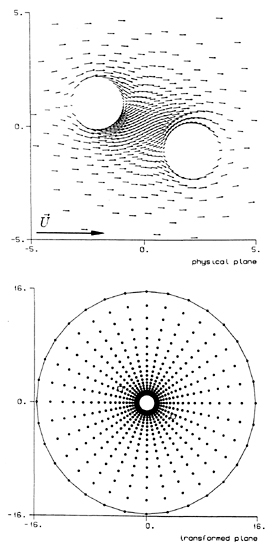
Figure 2: Unseparated flow around two staggered cylinders. The direction of the ambient flow is indicated by the big arrow. The arrow plot shows the velocity field calculated by equation (13). The start point of each arrow in the physical plane is the image of one mark (•) in the transformed plane. The image of the physical origin and infinity are marked with (○) and (□), respectively.

Figure 3: Force coefficients of two tandem circles at β=534 with the gap width d/a=4; drag and mass coefficients respectively in figure (a) and (b); (——): cylinder Nº1; (– – –): cylinder Nº2; (Δ): experimental data from (17); (□): drag due to friction (present method); (◇): drag due to pressure (present method); (○): total drag (present method); (∇): mass coefficient (present method); (–·–·–): experimental data from (18) at Re=2.5 · 104 and d/a=3 and 5.
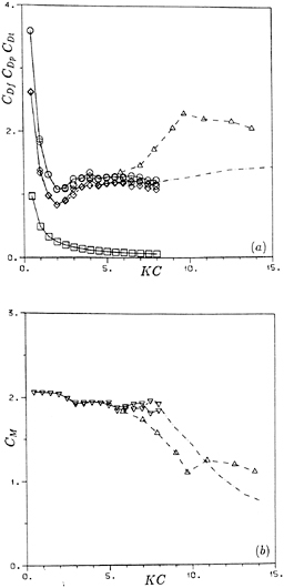
Figure 4: Force coefficients of two tandem circles at β=534 with the gap width d/a=8; drag and mass coefficients respectively in figure (a) and (b); (——): cylinder Nº1; (– – –): cylinder Nº2; (Δ): experimental data from (17); (□): drag due to friction (present method); (◇): drag due to pressure (present method); (○): total drag (present method); (▽): mass coefficient (present method); (–·–·–): experimental data from (18) at Re=2.5 · 104 and d/a=8.

Figure 5: Drag force signal (Fx) of two tandem circles with spacing d/a=6 in a steady ambient flow at Re=100; (——): upstream cylinder; (-------): dowstream cylinder.

Figure 6: Drag coefficients CD for two tandem cylinders with the spacing d/a=6; the empty marks are connected to the downstream cylinder; (– – –): experimental data from (24) for a single cylinder; (▽): experimental data from (22); (◇): experimental data from (18); (Δ): numerical results from (12); (□): present numerical results

Figure 7: Strouhal number of two side--by-side cylinders in a steady incident flow at Re=200; (×): experimental data reported by (21) and (25); (Δ): upper cylinder (present numerical results); (▽): lower cylinder (present numerical results); (○): numerical results from (12) for Re=200; (——): experimental data for a single cylinder reported by (24) for Re=200.
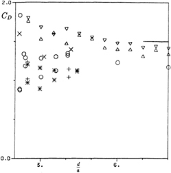
Figure 8: Drag coefficients of two side-by--side cylinders in a steady incident flow at Re=200; (Δ): upper cylinder (present numerical results); (▽): lower cylinder (present numerical results); (○): numerical results from (12) for Re=200; (+, ×, *): experimental data reported by (21) and (25) at Re=8 · 103, 2.5 · 104 and 6 · 104, respectively; (——-): experimental data for a single cylinder reported by (24) for Re=200.

Figure 9: Mean value of the lift coefficients of two side-by-side cylinders in a steady incident flow at Re=200; (Δ): upper cylinder (present numerical results); (▽): lower cylinder (present numerical results); (○): numerical results from (12); (+, ×, *): experimental data reported by (21) and (25) at Re=8 · 103, 2.5 · 104 and 6 · 104, respectively.
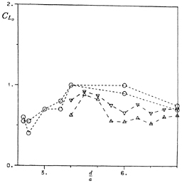
Figure 10: Amplitude of the oscillatory component of the lift coefficients of two side-by--side cylinders in a steady incident flow at Re=200; (Δ): upper cylinder (present numerical results); (▽): lower cylinder (present numerical results); (○): numerical results from (12).


