
Computation of Viscous Flow Around a Rudder Behind a Propeller: Laminar Flow Around a Flat Plate Rudder in Propeller Slipstream
H.Suzuki, (NKK Corporation, Japan)
Y.Toda (University of Mercantile Marine, Japan)
T.Suzuki (Osaka University, Japan)
ABSTRACT
The viscous flow computation of propeller-rudder interaction is presented through comparisons with experimental data including flow visualization and mean-flow measurements. The steady flow field is calculated by a viscous flow code coupled with a body-force distribution which represents the propeller. The transport equations are discretized using a staggered grid and the exponential scheme. The velocity-pressure coupling is accomplished based on the SIMPLER algorithm. Qualitative agreement is obtained between the calculations and the mean-flow data. Although the details of the flow field is different because of the laminar flow computation and numerical treatment, the computational results show the essential feature such as upward movement of propeller slipstream in port side vise versa in starboard side. The streaklines from one blade position are traced and compared with the flow visualization using dye and air bubbles. The results show very similar trends. Those comparisons show the conclusion that the present approach can simulate qualitatively the steady part of the flow field around a rudder in propeller slipstream.
NOMENCLATURE
|
CT |
=thrust coefficient |
|
DP |
=propeller diameter |
|
fbx |
=x wise body force per unit volume |
|
fby |
=y wise body force per unit volume |
|
fbz |
=z wise body force per unit volume |
|
fbθ |
=θ wise body force per unit volume |
|
J |
=advance coefficient (=VA/nDp) |
|
KT |
=thrust coefficient |
|
KQ |
=torque coefficient |
|
p |
=pressure |
|
Q |
=propeller torque |
|
Rn |
=Reynolds number (=VADP/ν) |
|
Rh |
=hub radius |
|
Rp |
=propeller radius (=Dp/2) |
|
T |
=propeller thrust |
|
u,v,w |
=velocity components in cartesian coordinates |
|
x,y,z |
=cartesian coordinates |
|
x,r,θ |
=cylindolical coordinates |
|
n |
=number of propeller revolution |
|
VA |
=propeller advance speed |
|
Greek symbols |
|
|
Г |
=circulation distribution |
|
ν |
=kinematic viscosity |
|
ρ |
=fluid density |
1.
INTRODUCTION
The interaction between a propeller and a rudder is one of the major problems from the viewpoints of not only maneuverability but also propulsive performance, so numerous studies have been performed for flow field around rudder behind a propeller without rudder angle.
(Nakatake's review of this topic1) Among those studies, the flow field is calculated mainly by invicid-flow method under the assumption that the interaction is invicid, and in theoretical works the shapes of trailing vortex are assumed comparatively simple such as only consideration of propeller-slipstream contraction (Tamashima et al.2, Ishida et al.3) . On the contrary, in experimental studies, it is reported that propeller slipstream is dramatically deformed by the rudder effect from the data of mean-flow measurement by Baba et al.4 and Ishida et al.3 and from the result of flow visualization of the propeller tip-vortex by Tanaka et al.5 and Tamashima et al.2.
Recently, a lot of fin type energy-saving devices which is installed on a rudder are proposed
and put to practical use. (for example, NKK-SURF6, IHI A.T.Fin7). For the better understanding and improvement of the performance of such devices, it is advisable to develop the calculation model which can express the phenomena which is observed in experiments.
On the other hand, with respect to the time-averaged flow of the propeller slipstream, it is reported that the computed propeller-hull interaction flow field by the method that propeller effect is represented by the body force distribution in the computation code of Navier-Stokes equation shows good agreement with the experimental result in propeller slipstream8,9.
In this paper, the flow field with a flat plate rudder is computed by the Navier-Stokes solver coupled with analytical prescribed body-force distribution as the simplest model of propeller-rudder interaction problem. And the result are compared with experimental data for similar condition carried out in circulating water channel. Although the details of the flow field is different because of the laminar flow computation and numerical treatment, it is appeared that the method can express phenomenon which appeared in experimental data with respect to time-averaged flow. A simulation of the streakline from a rotating point on the propeller plane is similar to the flow visualization result. Moreover half domain computation and full domain computation are carried out and compared. These results are almost same for present laminar and steady flow computation.
In the presentation of the results and the discussion to follow, a Cartesian coordinate system is adopted in which x-, y- and z- axes are in the direction of the uniform flow, starboard side of the rudder and upward respectively. The origin is at the intersection of the shaft center line and the propeller plane. The mean velocity components in the direction of the coordinate axes are denoted by u,v,w. Unless otherwise indicated, all variables are nondimentionalized using the propeller diameter Dp, propeller advance speed VA and fluid density ρ. In some part, the cylindolical (x,r,θ) coordinates in which x=x,y=rcosθ and z=rsinθ are used.
2.
EXPERIMENTS
Mean-flow measurements and flow visualization were carried out in NKK Tsu Ship Model Basin, circulating water channel to compare with computational results. Experimental results are shown first to explain the phenomena of propeller-rudder interaction.
2.1
Model Rudder, Propeller and Their Arrangements
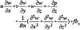
The principal dimensions of the propeller and the flat plate rudder are given in table 1. The leading edge and trailing edge of the 8mm flat plate rudder are tapered as shown in Fig. 1.
The arrangement of the flat plate rudder and propeller open boat with the propeller is shown in Fig. 2. The propeller open boat was attached front-side back so that the propeller shaft did not pass through the rudder. But this arrangement had a point that wake of the open boat was generated. So an extension shaft was attached to the propeller open boat so that the open boat did not have a large disturbance on the flow field. Length between propeller plane and the rudder leading edge was 0.30DP (66mm) and the propeller shaft center depth from the free surface is 1.50DP (330 mm) in order to minimize the free surface effect.
2.2
Mean-Flow Measurement
The device for measuring the propeller slipstream, which is unsteady flow field, should be preferably be carried out by a non-contact type Laser Doppler velocimetory or the equivalent; however, instruments of this type cannot be widely used now. Therefore, two spherical-type 5 hole pitot probes, one for the port and the other for starboard side of the center plane, were used in mean-flow measurements because it is easy to handle and able to measure time averaged velocities. Velocities were measured for the with and without rudder condition. The number of propeller revolution and the corresponding thrust and torque coefficients for both conditions are shown in table 2. Note that the thrust and torque for the with rudder condition are 4% larger and 2% smaller than those for the without rudder condition, respectively. It is similar as the other experimental data and might be due to the displacement effect of the rudder and the distortion of the trailing vortex geometry by rudder discussed later.
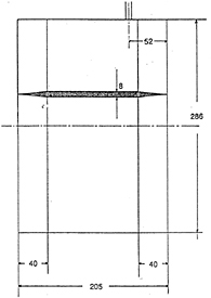
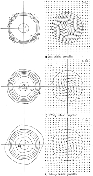
The mean-velocity field measurements were performed for both conditions and for three axial stations shown in Fig. 3. These locations were just behind propeller plane (x=0.125, 0.125DP downstream of propeller plane) , x=1.23 (in case of with rudder, the trailing edge of the flat plate rudder) and the position at x=2.0 (2DP downstream of the propeller plane.
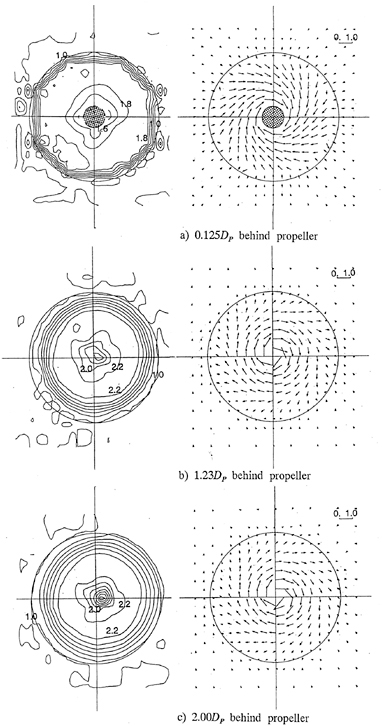
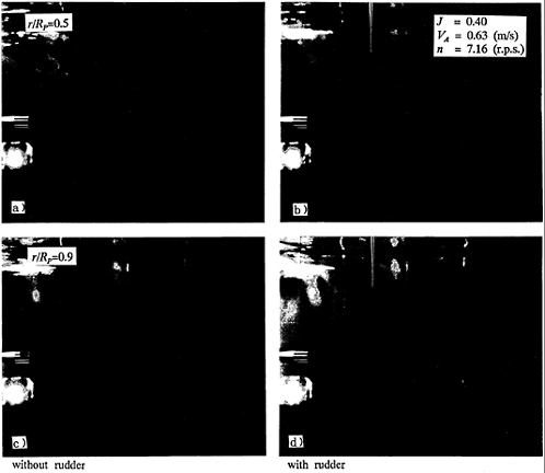
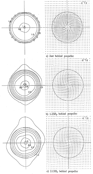
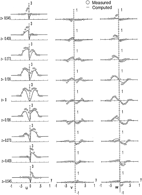
The results of the mean-flow measurement of the propeller slipstream are shown in Fig. 4 and Fig. 5 for the with and without rudder condition, respectively. The mean-velocity field without
propeller and rudder at first measurement station is shown in Fig. 6 in order to check the effect of the open boat. Although a small region where the velocity defect is observed and it is asymmetric, the flow field is seems to be almost uniform in the present experimental region. In Fig. 4, the time averaged propeller slipstream similar to a swirling jet is observed for the without rudder condition. From the cross-plane vectors, the swirl velocity is maximum just downstream of the propeller and decays gradually with downstream distance. The crossplane vectors outside the propeller slipstream at x=0.125 show the flow direction towards the shaft center. It shows the flow contraction by the propeller. The axial velocity is increased from x=0.125 to x=1.23 and decay very gradually. The concentration of the axial velocity contours near the propeller tip is the trace of the tip vortices and its associated vortex sheet, which diffuses with downstream distance.
For the with rudder condition shown in Fig. 5, very similar velocity distribution as that for the without rudder condition is observed at x=0.125. The diffusion of tip vortex sheet and so on are similar. However, the slipstream is clearly altered due to the rudder effect at the latter two stations. The slipstream moves upward (toward the free surface) in the port side and moves downward in the starboard side. The outer shape of the slipstream in one side altered from the half circle at x=1.23. It shows that the movement seems to be larger near the rudder surface. Tanaka et al.10 explained the phenomena by the mirror image vortex due to the rudder. The propeller slipstream shows complicated shape at x=2.0 and the outer shape is enlongated in vertical direction and almost same in horizontal direction as compared with that for the without rudder condition. The cross plane velocity is smaller and the axial velocity is a little bit larger for the with rudder condition. The overall results of mean-flow measurement show similar results of Baba et al4. and Ishida3 although the one measurement was carried out behind the hull.
2.3
Flow Visualization
Flow visualization was carried out for both with and without rudder condition. Streakline from one blade position was visualized by dye method according to Nagamatsu et al.11. The device is the tank which is attached on the boss part of the propeller and dye in the tank. When the propeller is rotating, water enters from boss part inlet and colored water go out from the small diameter tube which attached propeller trailing edge by their head difference. But this method can not be used for fast flow because dye defuses immediately. So, the number of propeller revolution n was selected as 7.16 (r.p.s.) and propeller advance speed VA was 0.63 (m/s) to keep the advance coefficient J same as in mean flow measurements.
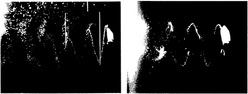
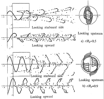
The results are shown in Fig. 7 for both conditions. The streaklines from r=0.5RP and r=0.9 RP are shown in figure; where RP is the propeller radius. For the without rudder condition (a) and c)), the helical streaklines are seen as usual and the streaklines are deformed drastically for the with rudder condition. It moves upward in port side and downward in starboard side. Note the transparent rudder enables to see streaklines in both side. The movement of streaklines is very similar to the tip vortex visualization by Tanaka et al5. shown in Fig. 8. In this figure, the air bubble method was used for visualization. The results for similar condition are shown in figure. The deformation of those streaklines is corresponding to the enlargement of slipstream in vertical direction.
In the experiment, the phenomena observed in the previous studies is reproduced for the flat plate rudder. It is explained by Tanaka et al.10 by images. So, if the nonlinear trailing vortex geometry including rudder effect is used for the calculation using iterative procedure, it can be expressed by invicid method. But, it seems difficult to treat the induced velocity at the vortex segment near the rudder. So, in this paper, the computation of Navier-Stokes equations for the time averaged flow field has been investigated if it can express the before mentioned phenomena or not.
3
COMPUTATION
3.1
Governing Equations and Computational Method
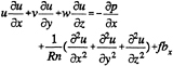
In this paper, the computation was carried out for the zero thickness flat plate rudder which had same profile as the rudder used in experiment and the time averaged flow using time averaged body force distribution following Stern et al.9. The computation was carried out for steady laminar flow case because the turbulence model in the slipstream was not clear, the present approach can not treat the complicated unsteady phenomena in the slipstream such as blade wake and so on and the grid number was limited due to the memory size of the computer. So, three-dimensional steady Navier-Stokes equations and the continuity equation are used for the governing equations. The equations are written in cartesian coordinates discussed in section 1 in the physical domain as follows;
(1)

(2)
(3)
(4)
where p is the pressure normalized by ![]() , Rn=VADp/ν is the Reynolds number defined in terms of VA,DP and molecular kinematic viscosity ν. The terms fbx, fby and fbz in the momentum equations are the components of the body force, normalized by
, Rn=VADp/ν is the Reynolds number defined in terms of VA,DP and molecular kinematic viscosity ν. The terms fbx, fby and fbz in the momentum equations are the components of the body force, normalized by ![]() and represent the influence of the propeller. These will be discussed subsequently.
and represent the influence of the propeller. These will be discussed subsequently.
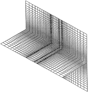
The equations are transformed into irregular orthogonal coordinates shown in Fig. 9. The transformed equations are discretized by exponential scheme 12 using the staggered grid in which pressure is defined at the grid point and the velocity components are defined at half grid shifted points in x,y and z direction for u,ν and w, respectively. The pressure-velocity coupling is accomplished based on the SIMPLER algorithm. The matrix is solved using tri-diagonal matrix solver and line-by-line iteration method. The steady converged solution was obtained by iterative procedure from the guessed initial condition (uniform flow except for the plate surface). After about 500 iterations, the converged solution was obtained.
103 was used for Reynolds number in the computation from the grid size discussed later. Note that the Reynolds numbers in the experiment are 2.4×10⁵ and 1.2×10⁵ for the mean-flow measurements and flow visualization, respectively.
3.2
Analytically-prescribed body force distribution
To represent the propeller effect in the numerical method, the body force fbx in axial direction and fbθ in circumferential direction are used corresponding to thrust and torque. Following the Stern et al.9, the body force fbx and fbθ are prescribed using the loading condition in the experiment shown in table 2. Although the computation was carried out for both with and without rudder condition and the loading conditions were a little bit different in experiment, the loading condition for without-rudder condition was used for both condition because the zero thickness plate rudder which had a small displacement effect was used in the computation. Of course, the interactive method using a invicid propeller theory is preferred and the body force should be the function of θ for the with rudder condition. But, because the computer program which can treat the nonlinear training vortex geometry for with rudder condition like the program of Ishii13 for the without propeller condition was not available, the same distribution as for the without rudder condition was used.
Following the noniterative calculation of Stern et al.9, the circulation distribution on the propeller blade of Hough and Ordway14 was used to determine body force.
The body force fbx and fbθ are written using the loading coefficient ![]() , torque coefficient
, torque coefficient ![]() and advance coefficient J (=VA/nDp) as follows;
and advance coefficient J (=VA/nDp) as follows;
(5)
(6)
(7)
(8)
where r*=(Y−Yh) / (1−Yh), Yh=Rh/RP and Y=r/RP; Rh is boss radius; RP is propeller radius; T is thrust; Q is torque, Δx means x direction grid size at propeller plane. And CT is easily calculated from KT .
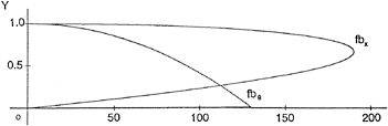
Body force distributions from KT,KQ and
J for without propeller condition in table 2 are shown in Fig. 10. In the present computation, propeller is assumed without boss. fbθ is non-zero from the equation (6) at r=0. But fbθ is thought to be zero at the shaft center as shown in figure. fby and fbz are decomposed from fbθ as follows.
fby=−fbθsinθ, fbz=fbθcosθ (9)
In the computation, the fbx,fby and fbz are given at the points where u,ν and w are defined, respectively, corresponding to the pressure points at the propeller plane. So, r and θ are calculated from y and z at those points and fbx and fbθ are calculated from eq.(5) through (8).
3.3
Solution domain and Computational Grid
In the computation, the detail propeller geometry, the thickness of rudder and the rudder stock were ignored. The arrangements of the propeller and the rudder is defined as follows; The propeller plane is x=0 and the propeller disk in which the body forces are non-zero is the circle whose radius is 0.5. With respect to the flat plate rudder, leading edge is x=0.3; trailing edge is x=1.23; upper edge is z=0.65; lower is z=−0.65, and it exists on y=0 in z-x plane. Those arrangement is same as that in experiment.
Two Solution domains are used for the computation. One is the half (starboard side) domain using symmetric condition with respect to the shaft center line for the present geometry written as follows;
u(x, y, z)=u(x,−y,−z)
ν(x, y, z)=−ν(x,−y,−z)
w(x,y,z)=−w(x,−y,−z)
p(x,y,z)=p(x,−y,−z) (10)
This computation was carried out first to save the memory size. In this case, The solution domain is [−3, 3.63], [−0.05, 3.0] and [−3.0, 3.0] in x,y and z directions, respectively. The other is the full (port and starboard sides) domain. The solution domain is [−3.0, 3.0] in y direction and the same for the other direction as the half domain. Computational grid of the former case is shown in Fig. 9. The grid system of latter case extended to negative y direction as same as positive y direction. The grid numbers are (63, 32, 61) in (x, y, z) direction, respectively for half domain computation and (63, 61, 61) for full domain computation. The minimum grid spacing is 0.01 at propeller plane, rudder leading edge and trailing edge in x directions, and 0.05 in y and z directions in the region where y or z is less than 0.7. This uniform grid size near the propeller circle in cross plane is chosen from experimental results. Axial body force (fbx) is embedded at x=0.005 and y and z direction body force (fby,fbz) at x=0 in x direction due to the staggered grid system. Note fby is given at ν point and fbz at w point at x=0.0.
3.4
Boundary Conditions
The boundary conditions are as follows;
-
on inlet plane x=−3.0, uniform flow condition is given. u=1.0, ν=w=p=0
-
on exit plane x=3.63, zero-normal(axial)-gradient condition is applied.
-
on the outer boundary in y direction y=±3.0, ∂(u,w,p)/∂y=0, ν=0
-
on the outer boundary in z direction z=±3.0, ∂(u, ν, p)/∂z=0, w=0
-
on the rudder surface, no slip condition and zero-normal-pressure-gradient condition are imposed. u=v=w=0.0 and ∂u/∂y=0
For the half domain computation, above symmetric condition eq(10) is used for u,w,p at y=−0.05 and ν at y=−0.025 by using u,w,p at y=0.05 and ν at y=0.025 of previous iteration except for on the flat plate rudder.
4.
COMPUTATIONAL RESULTS AND DISCUSSION
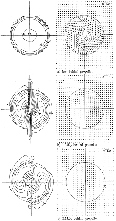
Axial velocity contours and cross flow vectors of half domain computation for the with and without rudder conditions are shown in Fig. 11 and Fig. 12, respectively. The results of full domain computation are shown in Fig. 13 and Fig. 14 for the with and without rudder conditions, respectively. The velocity distributions are drawn at three axial stations; a) at x=0.01 (just downstream of the propeller plane), b) x=1.23 (at rudder trailing edge), and c) x=2.13 (grid point near the station of experiment). From those figures, two computations show almost same results although the full domain computation show a little bit asymmetry with respect to the center line. So, for the present steady laminar flow computation, half domain computation can be used to get the very similar results by small computer as those of full domain computation. In the following, the results of full domain computation are discussed.
For the without rudder condition shown in
Fig. 13 a), b), c), the computational results show general feature of the propeller slipstream. The axial velocity is accelerated and the swirl velocity is produced by the propeller at x=0.01. The swirl velocity is maximum just downstream of the propeller and decays with downstream distance. At x=0.01, the flow toward the shaft center exists outside the propeller slipstream corresponding to the contraction. The axial velocity is increased from x=0.01 to x=1.23 and decay very gradually. The axial velocity contours also show the diffusion of the tip vortex sheet. So, the computation can capture the flow field qualitatively. In comparison with experimental results shown in Fig. 4, the acceleration of the axial velocity and swirl velocity are both underpredicted at just behind the propeller. It might be due to the coarse grid size at propeller plane and the effect of the boss. The body force distribution applied for this computation which is made based on the force measurement and Hough and Ordway circulation distribution also might be different from load distribution of mean-flow measurement condition. The acceleration and decay of the axial velocity is predicted fairly well if the underprediction at x=0.01 is considered. But the diffusion of the concentration of axial velocity contours near the propeller radius is faster than experiment. The reason is considered as the low Reynolds number computation and the numerical diffusion due to coarse grid in cross plane. The decay of the swirl velocity is much faster than that in experiment especially near the shaft center line. In experiment, the swirl velocity is larger as the position is closer to the shaft center line at all three stations. It suggests that the strong hub vortex exists, the diameter of its core is very small and its decay is slow. But in the computation, The large core of the hub vortex is observed at x=0.01 and decays very fast. It is due to the difference of Reynolds number and the coarse grid.
For the with rudder condition shown in Fig. 15 a), b), c), the computation also show the general qualitative feature of flow field. At x=0.01, the velocity distribution is almost same as that for the without rudder condition. The high velocity region moves upward in the port side and downward in the starboard side at the latter two stations. The cross plane vectors are smaller than those for the without propeller condition. In comparison with experimental results shown in Fig. 5, both axial velocity acceleration and swirl velocity are underpredicted similar as for the without rudder condition. At the rudder trailing edge, x=1.23, high velocity region has similar shape as the experimental high velocity region except near the flat plate. Near the flat plate, the cross plane velocity is small due to the laminar boundary layer and the present computation resolution. It might be the reason why the upper edge of the slipstream has different shape from the experimental results. The difference of the decay of the axial velocity contour concentration and the cross plane velocity between in experiment and in computation is almost same as for the without rudder condition. The change of the direction of cross plane vector from the without rudder condition to the with rudder condition is predicted fairly well, although the difference is observed in detail due to the thickness effect and so on. At x=2.13, comparing with the experimental results at x=2.0, the position of high velocity region is predicted fairly well, but the outer shape of the slipstream is different. The movement of the slipstream near the center plane is small due to the laminar boundary layer and wake and small cross plane velocity. So, the gap between port side and starboard looks small, but the gap of the high velocity region show similar trend. Note that the vortices whose turning direction is unti-clockwise are observed in the upper part of the port side and in the lower part of the starboard side. It is also observed in experimental result of Tanaka et al.10. It is also noted that the lower velocity region near the center plane at x=1.23 is observed in lower part of the port side and upper side of the starboard side in experiment. It might be the movement of divided hub vortex. This phenomena is also seen in the computational results, but the movement is small and not clear due to the laminar boundary layer and the diffusion of hub vortex.
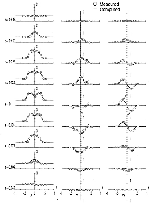
To compare the computation and experiment more precisely, the velocity profiles at nine heights at x=1.23 are shown in Fig. 15 and Fig. 16 for the without and the with rudder conditions, respectively. For the without rudder condition, the axial velocity and cross flow velocity are both underpredicted as discussed previously. For the axial velocity, the shape of the acceleration is well predicted. For ν and w, overall shapes are predicted, but the w for z=0 show clearly the much larger diffusion of the hub vortex. For the with rudder condition, the three velocity components are also underpredicted. The velocity outside the boundary layer at z=0.545 is not affected by propeller in the computation although the influence of the propeller is observed in experiment. It might be due to the underprediction of the cross flow velocity. At z=0.409, the high axial velocity in the port side is predicted although the extent and the magnitude are underpredicted. At z=0.273 and 0.136, the larger region of high axial velocity and higher
axial velocity in the port side than in the starboard side observed in experiment are predicted similar fairly well. Horizontal velocity is smaller for the with rudder condition compared with for the without rudder condition. It is similar with experiment. The profiles of the axial velocity are very similar with experiment. At z=0.0, the velocity defect due to flat plate rudder is over-predicted because of the laminar flow computation and the coarse grid. The velocity distribution of both experiment and computation has the symmetric feature written in eq.(10).
From Fig. 11 through Fig. 16, the present computation show the large diffusion and the underprediction of velocity. It might be improved by turbulence model for at least plate boundary layer and wake and the finer grid. It also might be effective to use the Euler code.
Fig. 17 and Fig. 18 show the result of streakline tracing from the rotating point at propeller plane which is rotating at the same speed as the propeller blade. It has been conducted to investigate the model of training vortices in invicid theory for the with rudder condition. The procedure is as follows; (1) from the 72 points at every 5 degree θ at prescribed r, the streamlines are traced with time step J/72 (n=1/J, where n is the number of propeller revolution in the computation DP=1.0, VA=1.0). (2) The points at propeller plane were numbered in the unti-clockwise (positive θ) direction from 0 to M from θ=0 and the 72nd point is same as the 0-th point. (3) For the streakline from 0-th point, the point at K-th time step on the streamline from K-th point (K=0,M) were drawn. Although the flow field is steady, the present streakline show the helical streaklines which are observed usually. In comparison with the flow visualization, the pitch of the helical streaklines is similar for both r=0.5RP and r=0.9RP for without rudder condition. It shows the pitch of the helical streakline is larger at r=0.5RP than r=0.9RP. For the with rudder condition shown in Fig. 18, the distortion of the helical streaklines are clear. It shows the helical streakline moves upward in the port side and downward in the starboard side. It also shows the low velocity region where the simulated air bubbles do not go further compared with outer part of the boundary layer. These streaklines show very similar phenomena as experimental results shown in Fig. 7 and Fig. 8. The streaklines which is observed from downstream show the enlargement of the slipstream in the vertical direction clearly.
Limiting streamlines on the flat plate rudder surface at the port side are shown in Fig. 19. The uniform flow direction is from left to right in this figure. Although computational grid is so coarse, it is suggestive that upward flow exists on the rudder surface at the port side. The direction of limiting streamlines is similar as the direction of tufts on the surface of flow visualization by Tanaka et al.10.
5.
CONCLUDING REMARKS
This work presents mean flow measurement data and flow visualization of the flow field around the rudder in the propeller slipstream. The numerical method and the computational results for the flat plate rudder behind the propeller which represented by body force distribution are also presented. Although the Reynolds number of the computation is small and the number of grid is limited, the salient feature of the flow field for the time-averaged flow field has been predicted by present approach. In detail, there is some discrepancy due to the laminar flow computation and the numerical treatment. The present approach can be extended easily for the flat plate rudder with angle of attack in propeller slipstream and the rudder with zero thickness fins.
Finally, some of the issues that must be addressed while further developing the present approach are as follows: improvement of accuracy in calculating the propeller flow field; introduction of appropriate turbulence model for at least the rudder boundary layer; including the rudder shape (thickness and so on) effects by using body-fitted coordinate system; using finer and appropriate grid for propeller flow field. Also of interest is to use present approach for the improvement of the invicid theory which treat the propeller-rudder interaction.
ACKNOWLEDGEMENTS
The authors wishes to thank Dr. Y.Kasahara and Mr. Y.Okamoto at NKK Tsu Laboratories for their valuable discussion and encouragement. It is noted that the numerical work in this study has been carried out on the CONVEX C-120 at NKK Tsu Laboratories and on the AV6220 at Kobe University of Mercantile Marine.
REFERENCES
1. Nakatake, K.: “On Ship Hull-Propeller-Rudder Interactions”, 3rd JSPC Symposium on Flows and Forces of Ships, 1989, pp231–259 (in Japanese)
2. Tamashima, M., and Yang, C.J., Yamazaki, R.: “A Study of the Flow around a Rudder with Rudder Angle behind Propeller”, Transactions of the West-Japan Society of Naval Architects, No.83 , 1992 (in Japanese)
3. Ishida, S.: “The Recovery of Rotational Energy in Propeller Slipstream by Fins installed after Propellers”, Journal of the Society of Naval Architects Japan, Vol.159, 1986 (in Japanese)
4. Baba, E., and Ikeda, T.: “Flow Measurements in the Slipstream of a Self-Propelling Ship with and without Rudder”, Transactions of the West-Japan Society of Naval Architects, No.59 , 1979 (in Japanese)
5. Tanaka, I., Suzuki, T., Toda, Y., and Kawashima, T.: “Flow visualization of propeller tip vorticties using air bubbles”, 8th Symposium on Flow Visualization, 1980 (in Japanese)
6. Okamoto, Y., Kasahara, Y., Fukuda, M., and Shiraki, A.: “Development of a Energy-saving Device NKK-SURF (Swept-back up-thrusting Rudder Fin)”, NKK TECHNICAL REPORT, No.132, 1990 (in Japanese)
7. Mori, M., Yamasaki, Y., Fujino, R., Ohtagaki, Y.: “IHI A.T.Fin–1st Report: Its Principle and Development-”, Ishikawajima-Harima Engineering Review, Vol.23, No.3 , 1983 (in Japanese)
8. Stern, F., Toda, Y., and Kim, H.T.: “Computation of Viscous Flow Around Propeller-Body Configurations: Iowa Axisymmetric Body”, Journal of Ship Research, Vol.35, No.2 June 1991
9. Stern, F., Kim, H.T., Patel, V.C., and Chen, H.C.: “A Viscous Flow Approach to the Computation of Propeller-Hull Interaction”, Journal of Ship Research, Vol.32, No.4, Dec.1988
10. Tanaka, I., Kawashima, T., and Toda, Y., “On Flow Field Stracture Near Free Surface At the Stern Of Ship Models ”, Journal of the Kansai Society of Naval Architects, Japan, No.180, 1981 (in Japanese)
11. Nagamatsu, N., and Shimizu, H.: “Study on Propeller Slipstream”, Journal of the Kansai Society of Naval Architects, Japan, No. 197 , 1985 (in Japanese)
12. Patanker, S.V.: “Numerical Heat Transfer and Fluid Flow”, McGraw-Hill, New York, 1980
13. Ishii, N.: “The Influence of Tip Vortex on Propeller Performance”, Journal of the Society of Naval Architects Japan, Vol.168, 1991 (in Japanese)
14. Hough, G.R., and Ordway, D.E.: “The Generalized Actuator Disk”, Developments in Theoretical and Applied Mechanics, Vol.2, Pergamon Ga., 1965, pp 317–336
15. Suzuki, H., Toda, Y., and Suzuki, T.: “Numerical Simulation of a Flow Field Around a Flat Plate Rudder in Propeller Slipstream”, Journal of the Kansai Society of Naval Architects, Japan, No.219, 1993 (in Japanese)
Table 1. Principal dimensions propeller and rudder
|
Propeller |
|
|
Number of Blades |
5 |
|
Diameter (mm) |
220.0 |
|
Pitch Ratio |
0.700 |
|
E.A.R. |
0.600 |
|
Boss Ratio |
0.170 |
|
Blade section |
MAU-M |
|
Direction of Rotation |
Right |
|
Rudder |
|
|
Thickness (mm) |
8.0 |
|
Chord (mm) |
205.0 |
|
Span (mm) |
286.0 |
Table 2. Propeller condition
|
Propeller condition |
|
|
VA (m/s) |
1.26 |
|
n (r.p.s.) |
14.32 |
|
J |
0.40 |
|
WITHOUT RUDDER |
|
|
KT |
1.91×10⁻¹ |
|
KQ |
2.54×10⁻² |
|
WITH RUDDER |
|
|
KT |
1.98×10⁻¹ |
|
KQ |
2.50×10⁻² |


Determination of Load Distribution on a Rudder in Propeller Slipstream Using a Nonlinear Vortex Model
B.Kirsten and S.D.Sharma
(University of Duisburg, Germany)
ABSTRACT
The ship rudder is a lifting surface of rather low aspect ratio. The free shear layers departing from the top and bottom edges of a rudder at an angle of attack tend to roll up even in way of the rudder, as can be easily observed by flow visualization in a cavitation tunnel, for instance. This already leads to a deviation from the simple linear dependence of lift force on angle of attack. The situation becomes much more complex for a rudder operating in a propeller slipstream where the root and tip vortices of the propeller periodically hit the rudder. To calculate the influence of the propeller on the rudder, the propeller slipstream is modeled by a vortex-line system of root and tip vortices; the rudder including the free shearlayer, by vortex-rings. This leads to a vortex-lattice method for stationary problems.
NOMENCLATURE
Coordinate Systems
Two different coordinate systems are used alternatively depending on convenience.
The non-rotating system Oxyz is righthanded, orthogonal, Cartesian, with origin O on (vertical) rudder axis at mid-height, x-axis in direction of uniform parallel (horizontal) inflow, and y-axis pointing upward. It is attached to the rudder but remains aligned to the inflow when the rudder is applied.
The rotating propeller-fixed system Oxrφ is cylindrical, righthanded, with origin O at intersection of (horizontal) propeller axis and blade generatrix, x-axis in direction of uniform parallel (horizontal) inflow, and r-axis coincident with first blade generatrix.
|
Main Symbols |
|
|
A |
Geometric influence coefficient matrix |
|
|
Radius vector |
|
|
Panel boundary vector |
|
cL |
Lift coefficient |
|
cTh |
Thrust loading coefficient |
|
D |
Propeller diameter |
|
J |
Propeller advance coefficient |
|
m |
Number of control points |
|
L |
Rudder chord length |
|
n |
Propeller rate of turn |
|
|
Field point vector |
|
R |
Propeller radius |
|
|
Vortex point vector |
|
|
Velocity of uniform parallel inflow |
|
|
Induced velocity |
|
z |
Number of propeller blades |
|
βi |
Hydrodynamic induced pitch angle |
|
Г |
Circulation |
|
γ |
Circulation density |
|
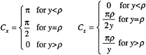
Δcp |
Load distribution normalized by stagnation pressure of uniform inflow |
|
|
Vortex segment |
|
Δξ |
Axial separation of helical vortices |
|
δ |
Rudder angle of attack relative to |
|
|
Velocity potential |
|
Λ |
Aspect ratio |
|
μ |
Dipole moment density |
|
ρ |
Radius of asymptotic vortex cylinder |
|
ρ |
Mass density of fluid |
1.
INTRODUCTION
The steadily increasing concern for safety and environment necessitates continued improvement of the maneuverability of ships. Typically, the control force in maneuvering is generated through a rudder located at the stern in the slipstream of a screw propeller. In order to clarify the complex hydrodynamics of this configuration, several comparative model experiments with a rudder in open water and propeller slipstream have been conducted, notably by Baumgarten (1979) in a towing tank and by Kracht (1990) in a cavitation tunnel.
These experiments show that the combined free-vortex sheet shed from the rudder side edges and trailing edge begins to roll up already in way of the rudder and evolves further downstream into two tip vortex braids. In addition, the free-vortex sheets of the propeller blades, already rolled up into discrete tip and root vortices, impinge upon the rudder (see Fig. 1).
A complete theoretical description of this incompressible viscous flow problem would require a solution of unsteady Navier Stokes equations with appropriate boundary conditions. An analytical solution being out of question for this complex geometry, some numerical approximation would need to be found by means of finite difference equations with a very fine discretization to catch the real vortex structure. The computational effort would be formidable. However, if viscosity is neglected (except in so far it is implicitly responsible for generation and shedding of vorticity), the problem can be handled efficiently by a singularity method which if formulated as an integral equation constitutes a solution of the Laplace Equation for a velocity potential. This reasonable and almost standard simplification in lifting surface problems at high Reynolds numbers is adopted in the present paper. Moreover, it is assumed that the effect of the propeller slipstream on the rudder, which amounts to a slowly time-varying inflow in the rudder-fixed reference system, can be approximated by discrete quasi-steady steps.
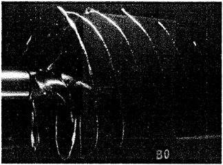
Figure 1. Rectangular streamline spade rudder at zero nominal incidence in the slipstream of a four-bladed propeller in a cavitation tunnel, reproduced from Kracht (1990).
For solving the potential equation, dipole singularities are distributed on the rudder center-plane and on the shear layer in the wake emanating from the side edges and the trailing edge; the propeller slipstream is idealized by discrete vortex lines. Boundary conditions necessarily imposed on the singular surfaces (no flux on the body and no force on the shed vortices) yield a nonlinear integral equation because the geometry of the shear layer is not known beforehand. Panelization of the singular surfaces reduces the integral equation to a system of (effectively nonlinear) algebraic equations which can be solved by iteration. A good overview of panel methods for vortex flows is given by Hoeijmakers (1989). Once the singularity strengths and locations are found, the velocity vector in the entire fluid domain including the boundary, i.e., the rudder surface can be calculated. Then also the pressure can be calculated everywhere by use of Bernoulli's equation.
Several singularity-based mathematical models for determining forces and moments on the propeller-rudder system as well as on the hull-propeller-rudder system have been formulated in the past, e.g., Brunnstein (1968), Tsakonas et al. (1970) and Klingbeil (1972). Due to the relatively low computer power available at that time these authors were forced to seek analytical solutions or estimates of the integrals involved as far as possible. An overview of the analytical approaches can be found in the books of Isay (1964, 1970). With present computing power a complex flow geometry can be better handled by a finer discretization of the flow boundary. Particularly suitable are panel methods which in case of simple singularities yield easily programmable algebraic equations, see, e.g., Belotserkovskii (1967).
The ship rudder is a classical lifting surface of small aspect ratio with a nonlinear lift characteristic arising from the influence of the separated secondary flow around the side edges. Such free-vortex sheets
shed from the side edges and subsequently rolling up have been computed by, among others, Schröder (1978) for low aspect-ratio wings and Wagner (1987), Wiemer (1987) and Haag (1988) for delta wings.
The problem becomes considerably more complex if the rudder is located in a propeller slipstream rather than in a uniform parallel inflow. The special case of a rudder in a nozzle was treated by Andrich (1989, 1990, 1991); however, the structure of free vortices shed by the propeller was prescribed on the basis of experimental observations (LDV measurements) rather than calculated as part of the complete solution.
The present work tries to compute the force-free configuration of the shear layers in the wake of the rudder as well as of the propeller, which necessitates solving a nonlinear integral equation. In distributing singularities on the shear layers of the rudder and the propeller particular attention must be paid to the vortex system of the propeller in way of the rudder.
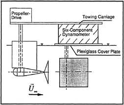
Figure 2. Schematic of reference model test in Duisburg Towing Tank (VBD): Rudder in slipstream, adapted from Baumgarten (1979).
Table 1. Propeller and rudder geometry and model test condition
|
Propeller: Wageningen B 4.55R |
||
|
Number of blades |
4 |
|
|
Diameter |
180 mm |
0.82 L |
|
Pitch ratio |
0.8 |
|
|
E.A.R. |
0.55 |
|
|
Hub ratio |
0.167 |
|
|
Rudder: Rectangular, modified NACA 0018 profile |
||
|
Chord |
220 mm |
1.0 L |
|
Span |
213 mm |
0.966 L |
|
Thickness |
40mm |
0.18 L |
|
Test condition: Propeller-Rudder in towing tank |
||
|
Thrust coefficient (without rudder) |
2.44 |
|
|
Advance coefficient |
0.444 |
|
|
Rudder LE to rudder stock |
70 mm |
0.32 L |
|
Rudder LE to propeller |
95 mm |
0.43 L (0.53 D) |
A model test (see Fig. 2 and Table 1) conducted by Baumgarten (1979) in the Duisburg Ship Model Tank (VBD) was used as bench mark for validating the present study.
2.
NONLINEAR VORTEX LATTICE METHOD
Choice of Singularity Method
The lift acting on a body at incidence in a stream can be explained by circulatory flow. In three-dimensional flows circulation may be generated by dipoles (oriented normal to the body surface). The other widely used type of singularity, namely, sources can only simulate the displacement effect of a body in a stream, but cannot satisfy the Kutta condition of smooth separation from the trailing edge which is the key to the generation of circulation. On the other hand, dipole distributions on the body surface can also simulate the displacement effect as long as the body has no sharp edges. For near a sharp edge the surface panels on opposite sides lie so close to each other that their induced velocities are almost self-canceling. The subdivision of a rudder surface, for example, in panels of constant dipole density would generate an almost singular system of algebraic equations with nearly zero elements on the side diagonals of the coefficient matrix.
Ship rudders typically have an aspect ratio from 1–2 and thickness ratio from 15–20 %. For such bodies the lift gain due to thickness effect is certainly not negligible, but presumably compensated for by an almost equal lift loss due to viscosity. By comparison, the nonlinear effect of separated flow around the side edges on the lift characteristic is much larger, as will be shown later. For this reason we simply place our dipoles on the rudder center-plane, ignoring not only viscosity but also thickness.
The model of flow around a rudder in slipstream is synthesized from two partial models: (i) rudder in uniform parallel inflow and (ii) propeller wake itself. Each partial model is separately validated by reference to available measurements. The ultimate criterion for the degree of detail to be simulated in each model is the adequate determination of pressure distribution on the rudder. This implies that the roll-up of the free-vortex sheets shed from the rudder side edges in way of the rudder itself must be simulated more precisely than the subsequent roll-up further downstream. For the same reason the bound vortices
of radially varying strength in the propeller blades and the associated wake vortex sheets with their immediate roll-up may be replaced by a simple horseshoe vortex for each blade.
In view of the rapid decay of the vortex-induced velocity with distance, each wake field is subdivided into a near field and a far field. In the near field the vortex is discretized and iteratively oriented to satisfy the no-force condition. In the far field (extending to infinity) an analytical truncation correction is applied rather than continuing the discrete vortex elements up to an arbitrary distance. Such far field approximation helps to reduce computing time and to prevent undue accumulation of numerical errors.
Definition of Boundary Value Problem
As explained in the Introduction, the Laplace Equation for the velocity potential
ΔΦ=0 (2.1)
subject to the kinematic condition of no flux through all vortex sheets
(2.2)
and to the dynamic condition of no force on all free vortex sheets
Δcp=0 (2.3)
is solved by a singularity method. In steady flow, this dynamic condition is equivalent to requiring that the free vortex sheet is a stream surface. The singularity method is a collocation method with singularities, comprising basic solutions of the Laplace equation, suitably located outside the potential flow domain. The free parameters of the singularity distributions (strengths or locations) are determined by the boundary conditions. In the present lifting body problem dipoles are distributed on the shear layer representing the rudder and its wake, see, for instance, Schröder (1979) and Hoeijmakers (1989). The perturbation velocity generated by a surface distribution of dipoles is given by the potential
(2.4)
Here μ is the dipole moment density on surface σ and ![]() is the radius vector from dipole point
is the radius vector from dipole point ![]() to field point
to field point ![]() .
.
The dipole layer induces at field point ![]() the velocity
the velocity
(2.5)
where s is the boundary of sigma.
The expression (2.4) for velocity potential is not directly involved in the determination of unknown dipole density μ. Rather, it is the total velocity which must satisfy the boundary condition (2.2) thereby yielding an integral equation
(2.6)
to be solved. Here ![]() is the velocity vector representing the uniform parallel inflow.
is the velocity vector representing the uniform parallel inflow.
Moreover, the dynamic boundary condition (2.3) must be satisfied, which means that for part of the singularity surface not only the dipole density but also its location is unknown beforehand. Hence, the integral equation to be solved is effectively nonlinear.
Numerical Solution
The nonlinear integral equation just derived is solved numerically by subdividing the bound and free vortex sheets into finite quadrilateral elements (panels) of constant dipole density. The approximation of constant density on each panel causes the surface integral in Equation (2.5) to disappear; the remaining line integral corresponds to the velocity field of a vortex line
(2.7)
of constant circulation Г=−μ on boundary s, see Martensen (1968). This is called a panel method of order zero or vortex-lattice method. In steady flow the circulation cannot change between successive panels on the free vortex sheet in the streamwise direction. Thus the free vortex surface is effectively modeled by vortex lines of constant strength which are at the same time also streamlines. Only the bound vortex surface comprises closed vortex rings, each of constant strength, whereby the side edge and trailing edge vortex rings extend to infinity, see Schröder (1979).
Since no general analytic solution exists for arbitrarily curved vortex lines, these are approximated by straight-line segments. Piecewise closed-form integration then reduces the integral equation to a summation equation.
Owing to the nonlinearity resulting from the unknown location of the free vortices, the above
equation has to be solved iteratively in a two-step procedure.
In preparation for the first step a stream surface is prescribed as location of the free vortex surface since this must be force-free. The kinematic boundary condition of no flux through the bound vortex surface then yields a linear system of algebraic equations for determining the unknown bound vortex strengths.
In the second step a new stream surface is calculated as next location for the free vortices. This is carried out as an Euler-Cauchy solution of an initial-value problem.
The above two-step procedure is repeated until the changes in bound vortex strengths and free vortex locations in two successive steps fall below prescribed error margins.
The propeller wake field is also calculated by the vortex lattice method. Instead of the vortex surface model used for the rudder, here each propeller blade including its wake is simply represented by a single horseshoe vortex of constant strength. The dynamic boundary condition of no force on the free vortices creates a nonlinearity also in this model which is handled by iteration as described above.
As stated previously, the velocities induced by the free vortices at any field point are computed by adding contributions from the near field and the far field. Discretization of the vortex lines is necessary only in the near field. Transition to the far field is so chosen that error in induced velocity at the field point of interest falls below a prescribed bound. In case of the rudder in open water the far-field free vortices are taken to be semi-infinite straight-lines. In case of the propeller alone the far-field free vortices are regular helices associated with blade tips and roots; for lack of an analytical expression for the velocity induced by a helical vortex line this field is idealized by two vortex cylinders, each of constant vortex density on its surface.
Induced Velocity Field of Vortex Line
Basis of a numerical solution in the vortex-lattice method is the discretization of curved vortex lines into straight vortices. Each vortex line is replaced by a finite number of straight-line segments so that the integral equation reduces to a summation equation.
According to Biot-Savart's Law a line element ![]() of an arbitrarily curved vortex line of constant circulation Г induces at an arbitrary field point
of an arbitrarily curved vortex line of constant circulation Г induces at an arbitrary field point ![]() the infinitesimal velocity:
the infinitesimal velocity:
(2.8)
where ![]() is the radius vector from a point
is the radius vector from a point ![]() on the vortex line to the field point
on the vortex line to the field point ![]() .
.
This expression can be integrated in closed form only for a straight-line segment or for a closed circular ring, in the latter case only for a field point at the center.
A straight vortex line of constant circulation Г, connecting points ![]() and
and ![]() , (subsequently called vortex segment) induces at an arbitrary field point
, (subsequently called vortex segment) induces at an arbitrary field point ![]() in 3D space the velocity
in 3D space the velocity
(2.9)
which can be expressed in closed form as
(2.10)
where the vector ![]() represents the vortex segment, and the vectors
represents the vortex segment, and the vectors ![]() and
and ![]() are the radius vectors from its endpoints to the field point. In particular, for a semi-infinite straight vortex extending from
are the radius vectors from its endpoints to the field point. In particular, for a semi-infinite straight vortex extending from ![]() via
via ![]() to infinity the expression reduces to
to infinity the expression reduces to
(2.11)
Note that ![]() here is not the endpoint but only a waypoint on the vortex segment.
here is not the endpoint but only a waypoint on the vortex segment.
If the field point lies on the vortex segment itself, the integral in (2.9) becomes singular; taking its Cauchy principal value, the induced velocity is found to be zero.
In numerically evaluating the summands of the induced velocity at any field point the following approximation is used to take advantage of the strong decay with distance from the vortex segment. If ![]() , then the velocity induced by the vortex segment (VS) is taken to be
, then the velocity induced by the vortex segment (VS) is taken to be
(2.12)
with the long-range field-point vector ![]() .
.
The magnitude of the difference between the exact solution for the induced velocity (2.10) and its
approximation (2.12) normalized by the magnitude of inflow velocity ![]() is defined as an error bound:
is defined as an error bound:
(2.13)
Estimated on the basis of this error bound, the minimum value for the distance beyond which the approximation may be used is found to be:
(2.14)
3.
RUDDER IN UNIFORM PARALLEL INFLOW
Bound and Free Vortex Sheets
The rudder skeleton surface is subdivided into quadrilateral panels, see Fig. 3. As the vortex segments are chosen to lie on the panel boundaries the geometrical grid is identical to the vortex grid. The control points lie at the intersections of the bisectors of opposite edges. The cross-product of these bisectors defines the panel plane; in case of warped panel, a surrogate plane.
Since the velocity field is explicitly required only at the location of the rudder, the roll-up of the side-edge vortices need not be fully simulated behind the trailing edge. Moreover, the free-vortex field is subdivided into a near field and a far field, the borderline lying downstream at the transition from finite vortex segments to the semi-infinite vortex.
For estimating the borderline between near field and far field the entire bound and free vortex sheet can be replaced by a horseshoe vortex since the free vortex sheet rolls up downstream into two tip vortices of equal but opposite circulation. For reasons of symmetry the two free vortex lines of the horseshoe vortex form at infinity a pair of straight-lines lying in a plane at an angle to the uniform parallel inflow which is less than the rudder angle of incidence.
The distance ![]() of the field point from the starting point of the semi-infinite vortex (VH) is determined by estimation so as to ensure that the magnitude of the velocity
of the field point from the starting point of the semi-infinite vortex (VH) is determined by estimation so as to ensure that the magnitude of the velocity ![]() induced by the semi-infinite vortex at the rudder trailing edge is less than a prescribed error bound εFar,VH. Only up to this point does the vortex line, as a chain of finite straight segments, need to be aligned to the flow. The error bound εFar,VH is defined as the ratio of the magnitude of velocity
induced by the semi-infinite vortex at the rudder trailing edge is less than a prescribed error bound εFar,VH. Only up to this point does the vortex line, as a chain of finite straight segments, need to be aligned to the flow. The error bound εFar,VH is defined as the ratio of the magnitude of velocity ![]() induced by the semi-infinite vortex to the magnitude of velocity
induced by the semi-infinite vortex to the magnitude of velocity ![]() of uniform parallel inflow.
of uniform parallel inflow.
(3.1)

Figure 3. Vortex lattice model of rudder: (a) Initial configuration of discrete panels representing rudder and its vortex wake comprising trailing edge and side edge separation, (b) Configuration for computing circulation, (c) Configuration for computing velocity.
The minimum distance between the starting point of the semi-infinite vortex downstream from the rudder trailing edge is then given by:
(3.2)
Here v=π−52º is the angle between vortex axis and field-point vector at which the induced velocity of a semi-infinite vortex has a maximum. The circulation Г of the rudder, considered as a flat
plate with a 2D lift coefficient gradient cL=2π, can be estimated to be
Г=πLU∞ sin(δ), (3.3)
where L is the chord length. Substitution of this value into Equation (3.2) yields the following minimum distance between a field point on the rudder trailing edge and starting point of the semi-infinite vortex:
(3.4)
According to this estimate, for a rudder angle δ=15º and velocity error bound εFar,VH=1%, for instance, the minimum distance to far-field borderline becomes ![]() .
.
Circulation of Bound Vortex
In principle we have to solve a nonlinear system of equations with two sets of unknowns, namely, circulations of the bound vortices and locations of the free vortices. As stated above, the locations of the free vortices have to be iteratively estimated. Then the no-flux condition on the rudder requires that at each control point the total velocity induced by all the vortices ![]() must yield together with the inflow velocity
must yield together with the inflow velocity ![]() a zero component along the normal
a zero component along the normal ![]() to the panel surface:
to the panel surface:
(3.5)
Thus the problem is reduced to the following system of algebraic equations:
where Aν,μ is the geometrical influence coefficient matrix, Гμ are the unknown circulations of the panel vortex rings, and m is the number of control points. This diagonally dominant set of equations is solved by a Gauß-Seidel algorithm.
Next, the previously estimated locations of the free vortex lines must be checked and, if necessary, corrected as explained in the next sub-section. After a necessary correction the circulations of the bound vortices must be recalculated. This iteration must be repeated until all prescribed error bounds are attained.
Elements of the coefficient matrix A are computed by adding the contributions of all vortices associated with a panel. Closed vortex rings on the bound vortex sheet comprise just four panel edge vortex segments, whereas the boundary panels comprise three bound vortex segments and two chains of free vortex segments extending downstream to infinity. In other words, boundary panels are represented by horseshoe vortices. Hence, there lie two counter-oriented vortices of, in general, unequal circulation on each common edge of neighboring panels on the bound vortex surface; on the free vortex surface this holds only for edges in the stream wise direction, see Fig. 3b. Once the circulations have been determined, for further computations the collinear edge vectors are added with the convention that positive sign points in the coordinate direction, see Fig. 3c.
Location of Free Vortices
There must be no pressure jump across the free vortex layer. It follows that the the free vortex surface coincides with a stream surface and that free vortex lines coincide with streamlines. The streamlines are calculated iteratively by an Euler-Cauchy algorithm. Starting from the rudder leading edge, each time an entire transverse row of free vortex segments (ending roughly in a plane normal to the inflow) is relocated; then all downstream nodal points of each free vortex line are displaced by the difference vector between the new and old locations of the last relocated vortex segment. When, marching downstream, this operation has been done for all transverse rows the whole free vortex lattice is realigned to the flow. Now, the bound vortex circulations are redetermined as described above. This two-step iterative procedure is truncated when the prescribed error bounds for the circulation of bound vortices and the location of free vortices have been reached.
The Euler-Cauchy single-step procedure was chosen here because the velocity field for computing new streamlines is reasonably available only at discrete points, namely, the nodes of the given vortex lines. Of course, in principle the induced velocity could be calculated at any arbitrary point, but physically meaningful results can be expected only either outside the shear layer or exactly on the vortex lines. Moreover, the continuously curved vortex lines have been approximated by straight segments whose ends only lie on the original lines.
The idealization of the free vortex field by vortex lines is adequately accurate as long as the separation between the various turns of the rolled-up vortex surface is larger than the neglected thickness of the shear layer. Furthermore, the transverse distance between vortex lines must be kept sufficiently small so that the planes connecting neighboring vortex segments do not intersect the rolled-up vortex sheet.

Figure 4. Computed bounded and free vortex sheets of a rectangular rudder in uniform parallel inflow (Λ=0.966; δ=15 deg).
Finally, it is noted that the last downstream semi-infinite straight vortices are simply assumed to be aligned to the uniform parallel inflow.
Lift and Pressure Distribution
Once the strengths of bound vortices and the locations of free vortices are determined the induced velocity can be calculated at any field point of the flow by Biot-Savart's Law.
The force and moment on the rudder can be found by applying Kutta-Joukowski 's Law. For this purpose, the effective velocity ![]() at the center of each bound vortex
at the center of each bound vortex ![]() is determined as the sum of inflow velocity
is determined as the sum of inflow velocity ![]() and the induced velocity
and the induced velocity ![]() ; here
; here ![]() is any panel edge vector and Г the sum of circulations of adjacent panel vortex rings on the rudder skeleton surface. The local lift force
is any panel edge vector and Г the sum of circulations of adjacent panel vortex rings on the rudder skeleton surface. The local lift force ![]() on the vortex considered is proportional to the cross product of effective velocity vector and vortex vector:
on the vortex considered is proportional to the cross product of effective velocity vector and vortex vector:
(3.7)
where ρ is the mass density of the fluid. This local force can be resolved along any desired direction, for instance, normal to the rudder center-plane.
The local normal force divided by the panel area yields the pressure difference across the rudder assumed constant over any single panel; it is computed as follows. Each individual force according to Equation (3.7) is distributed as uniform pressure over two adjacent panels. For any single panel the sum of contributions from all edges yields the total pressure difference (between pressure side and suction side). The side edges and the trailing edge carry no vortices and, hence, do not contribute to the forces. Each leading edge vortex bounds only one panel so its force is distributed over this one panel only.
An alternative approach would be to first calculate the velocity difference across the rudder at any control point and then via Bernoulli 's Equation the corresponding pressure difference. It would require the conversion of edge vortices into a surface distribution of vorticity on the panel. This method is believed to be equivalent but awkward and, hence, is not used here.
Fig. 5 shows clearly the effect of the free vortex surface, which separates from the side edge and rolls up as seen in Fig. 4, on the load distribution over the rudder center plane. With increasing distance from the leading edge the spanwise variation of pressure difference deviates more and more from the classic elliptic distribution.
This load distribution was calculated using an equidistant grid of 40*20 elements in spanwise and chordwise directions on the rudder skeleton plane and 32 equidistant element rows behind the trailing edge up to a distance 1.6L downstream. This chosen near-field length follows from a velocity error bound εFar,VH=1 % along with the measured lift coefficient gradient 0.7π. A closer estimate than in the example following Equation (3.4) was necessary since the computing time increases as the square of the number of elements of the free vortex surface.
Total force coefficients for the rudder in any direction (lift, drag and cross-force) are easily obtained by summing up the local forces on all bound vortices. Fig. 6 shows the thus calculated lift characteristic of the reference rudder as well as a linear approximation and two sets of measurements. Strikingly, the present calculation agrees better with measurements on a thin flat plate with sharp leading edge than with those on the reference streamline
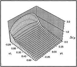
Figure 5. Computed normalized load distribution on the skeleton plane of a rectangular rudder in uniform parallel inflow (Λ=0.966; δ=15 deg).

Figure 6. Lift characteristic of a rectangular rudder (Λ=0.966) in uniform parallel inflow.
rudder of 0.18 thickness ratio. The measurements shown for the thin plate stem from Schlichting and Truckenbrodt (1969, p. 73). The lift coefficient gradient for a thin flat plate according to linear theory is c'L=πΛ/2 for aspect ratio Λ<1 and, hence, c'L=1.52 for the present case.
4.
PROPELLER SLIPSTREAM
Surrogate Horseshoe Vortex
Experiments reveal that the rudder is hit by already rolled-up propeller tip and root vortices, see Fig. 1. These vortices are, therefore, idealized as vortex lines in order to estimate the effect of propeller slipstream on the rudder. They are connected upstream by a bound vortex in each propeller blade and extend downstream to infinity. The bound vortex is located at the quarter-chord line of the blade skeleton surface. Although the root vortices seem to join into a single hub vortex, they are retained as individual vortex lines. This is necessary if induced velocities need to be determined within the streamtube formed by the root vortices, see Fig. 7.
According to measurements by Andrich (1989) the tip vortex is already fully developed within a quarter turn of the propeller. This is due to the steep drop of bound circulation near the tip. In any case, it happens well ahead of the rudder and, hence, we refrain from detailed modeling of the propeller flow and of the roll-up of its free vortex sheet. For consistency, the root vortices are assumed to be also fully rolled up into vortex lines before reaching the rudder.
As in the case of the flow around the rudder, the no-force condition on free vortex lines of a priori unknown location renders nonlinear the integral equation for determining propeller-blade bound circulation. Hence, a similar solution procedure is used here, of course, in the propeller-fixed coordinate system. However, for simplicity, two different vortex models are used for determining the circulations of bound vortices and the locations of free vortices within the horseshoe vortex system: For the former, a lifting surface model albeit with free vortices located on a fixed regular helical surface; for the latter, a lifting line model with free vortices iteratively aligned to the flow.
The propeller wake field is subdivided into a near field and a far field. In the near field discrete vortex lines are aligned to the resultant velocity field. For numerical reasons curved free vortex lines are approximated by straight vortex segments. The downstream continuation to infinity is modeled by a semi-infinite vortex cylinder (see Fig. 7) rather than by semi-infinite discrete lines as was the case for the rudder. Hence, in the far field discrete tip and root vortices are replaced by two semi-infinite circular vortex cylinders, each with a uniform vortex density on its surface. This far-field approximation is motivated by the fact that propeller tip and root vortices, for reasons of symmetry, ultimately lie on regular helical lines at downstream infinity, but no analytical solution is available for semi-infinite helical vortex lines as a convenient truncation correction.
The velocity field induced by a semi-infinite vortex cylinder can be expressed as a double integral, i.e., in axial and circumferential directions. At least the first integration can be done analytically, the second is performed by a Romberg quadrature.
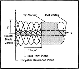
Figure 7. Vortex model of propeller slipstream comprising tip and root helical lines in the near field and cylindrical sheets in the far field.
The transition point from vortex segments to the vortex cylinder is determined such that the velocity error at any given field point resulting from the spreading of discrete line vortices on to the cylinder surface is less than a prescribed tolerance.
The velocity induced by a vortex cylinder at any arbitrary field point is according to Biot-Savart's Law given by:
(4.1)
Using a relative Cartesian coordinate system, whose x axis coincides with the cylinder axis and originates at the beginning of the cylinder, the components of the vortex element vector can be expressed as
(4.2)
and those of the radius vector ![]() from vortex element point
from vortex element point ![]() to field point
to field point ![]() as
as

(4.3)
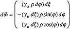
The uniform vortex density of the vortex cylinder has the components ![]() in the axial direction and
in the axial direction and ![]() in the circumferential direction, where z is the number of blades, Гz the circulation of a propeller blade tip/root vortex, ρ tan(βi) the hydrodynamic induced pitch, and ρ the cylinder radius. The determination of hydrodynamic induced pitch will be explained in the next sub-section.
in the circumferential direction, where z is the number of blades, Гz the circulation of a propeller blade tip/root vortex, ρ tan(βi) the hydrodynamic induced pitch, and ρ the cylinder radius. The determination of hydrodynamic induced pitch will be explained in the next sub-section.
After analytical integration in the axial direction the velocity induced by the semi-infinite vortex cylinder is found to have the following components:
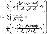
(4.4)
where
and ![]() is the absolute value of the projection of vector
is the absolute value of the projection of vector ![]() onto the yz-plane. For reasons of symmetry, the integration in the circumferential coordinate needs to cover only half the interval, that is, 0<φ<π.
onto the yz-plane. For reasons of symmetry, the integration in the circumferential coordinate needs to cover only half the interval, that is, 0<φ<π.
The total far field of the propeller wake is the sum of the contributions of the two semi-infinite vortex cylinders (VC) representing the tip and the root vortices.
We now seek a minimum distance ![]() between the field point and the far field such that the normalized velocity induced by the far-field model is less than an error bound
between the field point and the far field such that the normalized velocity induced by the far-field model is less than an error bound
(4.5)
Only within this range is it necessary to discretize the vortex lines of the propeller wake and to align them to the flow. Only the axial component of the induced velocity is considered for the purpose of this estimate since the radial and circumferential components are negligible by comparison. The estimate yields a minimum distance as the following function of propeller radius R, thrust loading coefficient cTh, and normalized velocity error bound εFar,VC:
(4.6)
In the iterative no-force alignment of the free vortex segments of propeller wake a transition range ![]() ahead of the vortex cylinders is specially considered. This is the distance between the last
ahead of the vortex cylinders is specially considered. This is the distance between the last
aligned vortex segment of the near field and the beginning of the far field. In this transition range the discrete vortex segments are just located on regular helices of same radius as the far-field cylinder. The size of the transition range is determined such that the error resulting from substituting a uniform vortex cylinder for discrete helical vortices is less than a relative velocity error bound
(4.7)
This estimate is obtained by comparing the velocities induced in the meridian plane of the vortex cylinder by a discrete vortex and and a vortex layer, both lying on the cylinder surface. Treating this as a 2D problem the following estimate is obtained:
(4.8)
This means that every individual vortex line must be continued as a chain of discrete vortex segments over an axial range ![]() between the end of the near field and the beginning of the far field. The axial separation of the vortex lines corresponds to the width of the vortex layer Δξ and can be expressed as a function of induced hydrodynamic pitch ρ tan(βi), cylinder radius ρ, and number of blades z:
between the end of the near field and the beginning of the far field. The axial separation of the vortex lines corresponds to the width of the vortex layer Δξ and can be expressed as a function of induced hydrodynamic pitch ρ tan(βi), cylinder radius ρ, and number of blades z:
(4.9)
In the chosen reference case with a loading coefficient cTh=2.44 the distance from field point to far field must be at least ![]() R for a normalized velocity error bound εFar,VC =0.01. When aligning the free vortices, this distance must be increased by the transition range, which for a four-bladed propeller operating at advance coefficient J=0.444 must be at least .
R for a normalized velocity error bound εFar,VC =0.01. When aligning the free vortices, this distance must be increased by the transition range, which for a four-bladed propeller operating at advance coefficient J=0.444 must be at least . ![]() For the latter estimate the hydrodynamic induced pitch far behind the propeller was taken, on the basis of momentum theory, to be ρ tan(βi)=0.262R, see also next sub-section. This leads to an axial separation of vortices equal to Δξ=0.412 R.
For the latter estimate the hydrodynamic induced pitch far behind the propeller was taken, on the basis of momentum theory, to be ρ tan(βi)=0.262R, see also next sub-section. This leads to an axial separation of vortices equal to Δξ=0.412 R.
These values were used to compute the circumferentially averaged induced velocities due to the propeller at two axial locations 0.53 D and 1.75 D behind the propeller corresponding to rudder leading edge and trailing edge, respectively, in the reference case, see Fig. 8.
Circulation of Bound Blade Vortex
The circulation and the starting points of tip and root vortices of each propeller blade are determined by reducing the vortex lattice with radially varying circulation to a surrogate simple horseshoe vortex, see Schlichting (1969, p. 32).
The location of each free vortex line depends

Figure 8. Computed propeller induced velocity components in the slipstream at rudder LE (left) and TE (right) (Wageningen B4.55R: P/D=0.8; cTh=2.44).
on the starting point as well as on the circulation. Hence, the propeller thrust coefficient cTh is also calculated from the vortex lattice in order to adjust the calculated circulation in proportion to the thrust measured on the propeller (in an open water model test). This simple adjustment is permissible since by Kutta-Joukowski's Law the lift is proportional to the circulation and, hence, also the thrust coefficient. Starting points of the tip and root vortices are not too sensitive to the circulation and are, therefore, not adjusted.
The constant circulation of the surrogate horseshoe vortex is taken equal to the peak value of the radially varying circulation in the vortex lattice. The width of the surrogate horseshoe vortex and, hence, the starting points of tip and root vortices are so chosen that the integrals under the curve of circulation as a function of radius between the peak value and the inner and outer endpoints, respectively, remain unchanged, see Fig. 9.
The radially varying bound circulation is determined as follows. The propeller blade is idealized by an array of radially neighboring horseshoe vortices, each with a bound part on the blade skeleton surface and a free part in the wake, see Fig. 10. The bound radial segment is located at quarter-chord from blade leading edge. The free segments start at the blade trailing edge and extend sufficiently far downstream on regular helices of pitch angle tan(βi). The unknown circulations of this vortex lattice are determined by satisfying the no-flux condition on the blade skeleton surface at one control point at threequarter-chord from the leading edge within each horseshoe.

Figure 9. Radially stepped bound circulation on propeller blade and surrogate single horseshoe vortex.

Figure 10. Vortex lattice model of propeller blades and their vortex wake sheets for computing radial variation of bound circulation.
The aforesaid pitch angle is found from an extension of Rankine's momentum theory to depend on local radius r/R, advance coefficient J, and thrust loading coefficient cTh:
(4.11)
see Ulrich and Danckwardt (1956).
Location of Tip and Root Free Vortices
As in case of the rudder, propeller wake is subdivided into a near field and a far field. Unlike the rudder, here the flow is steady in a rotating propeller-fixed system only. The basic flow now includes an angular component so that during the iterative alignment of free vortices in the near field the displacement vector from old to new vortex location cannot simply be superimposed onto the remaining downstream vortex segments. The length of the vortex segment remains unchanged during all corrections in the near field. In the far field, as stated earlier, the helical vortex lines are smeared out on the surface of a semi-infinite circular cylinder. Their constant radius and pitch are found by iteration.
The iteratively corrected new location of the free vortices is calculated in the near field by the single-step Euler-Cauchy algorithm just as in case of the rudder. This is done in an iterative loop starting at the bound vortex in the blade and marching downstream one transverse array (comprising one tip and one root vortex segment per blade) at a time.
Each free vortex segment is realigned to the flow found by averaging the velocities calculated at the last locations of its two endpoints. The remaining downstream vortex segments are provisionally displaced along helical surfaces of locally constant pitch as well as radially in proportion to the local radius so as to close the gaps created by the previous operation.
Final operation in the iterative loop is the adjustment of the semi-infinite vortex cylinders constituting the far field. The new radius (as well as pitch) is set equal to the average of its old value and the new value of the last realigned near-field segment. In the transition range between near field and far cylinder the radius and pitch of each vortex segment is found by linear interpolation to ensure continuous connection.
The above iteration is continued until the deviations in the vortex segment locations of the near field as well as of the far field between two successive steps become less than a prescribed error bound.
5.
EFFECT OF PROPELLER ON RUDDER
In a slipstream the rudder is subject to a periodic flow at blade frequency (equal to propeller rate times number of blades). The periodic effect is reflected in the free vortex lines of the propeller wake hitting the rudder. Since the hydrodynamic pitch is quite low, successive propeller vortices lie close to each other compared to rudder size. Hence, the periodic variation of velocity on the rudder surface is relatively small and is felt only in a narrow zone.
The pressure field on the rudder is obtained essentially by superimposing the vortex models of the rudder and the propeller wake. In order to find the periodic effect of the free propeller vortices on the rudder to a first approximation, the pressure field is considered as a function of relative blade position. More precisely, it is calculated individually for a finite number of values of circumferential angle assuming quasi-steady flow in the non-rotating coordinate system Oxyz. The range to be covered equals one propeller turn divided by the number of blades, corresponding to a full period of inflow.
The rudder and its wake including side edge separation are modeled, as above, by vortex surfaces and subdivided into panels carrying transverse dipoles of constant surface density or, equivalently, vortex rings of constant circulation. Thanks to the assumption of quasi-steady flow, vortex rings on boundary panels reduce to horseshoe vortices extending downstream to infinity. Their free vortex lines are discretized as chains of straight vortex segments the last of which is semi-infinite.
The propeller wake is simulated by helical blade tip and root vortices ending in semi-infinite
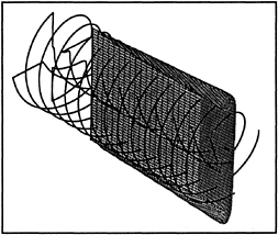
Figure 11. Computed vortex lattice of the rudder (Λ=0.966; δ=5 deg; D/l=0.82; φ=0 deg) with superimposed computed propeller vortices (Wageningen B4.55R: P/D=0.8; cTh=2.44).
cylinders. Their circulations and locations are taken unchanged from the open-water computation. This means that the obstruction of the slipstream by the rudder is ignored.
Fig. 11 shows a computed vortex lattice of the propeller-rudder system.
Fig. 12 shows, for the two extreme relative positions of a four-bladed propeller, the computed normalized load distribution generated on the rudder by the propeller wake. Note that the rudder is at zero angle of attack. The pressure difference peaks in way of the propeller wake vortices arise from singularities in the velocity field when the field point approaches a potential-vortex axis. However, the spurious peaks largely cancel each other out so that the effect on integral values is much less serious as will be seen shortly.
Fig. 13 shows the computed normalized load distribution on the rudder at 15 deg angle of attack without and with propeller wake, the latter for a single relative position of the blades. The strong effect of propeller wake on the mean value of the load as well as on its chordwise and spanwise distribution is evident.
Fig. 14 shows the computed lift characteristic of the reference rudder in propeller slipstream, obtained by summing local lift forces over the rudder surface and averaging over one period. For comparison, two sets of model test measurements are also included. The expected increase in rudder load as a result of propeller wake is generally confirmed. However, with increasing incidence the discrepancy between computation and model test increases up to about 30 % at 20 deg rudder angle. Much of it seems to be the result of ignoring rudder thickness effects as already evident in Fig. 6.
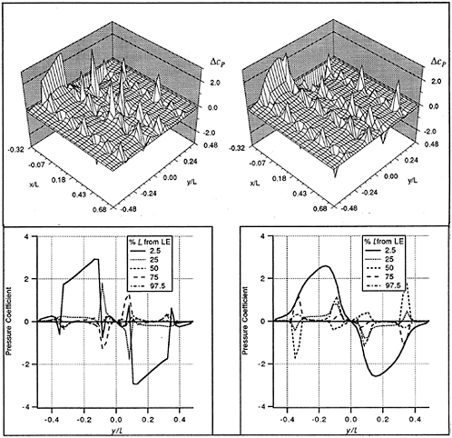
Figure 12. Computed normalized load distribution on the skeleton plane of a rectangular rudder in slipstream (Λ=0.966; δ=0deg;D/l=0.82).
Top left: Perspective view, φ=0 deg, Top right: Perspective view, φ=45 deg
Bottom left: Cross sections, φ=0 deg, Bottom right: Cross sections, φ=45 deg
6.
SUMMARY AND CONCLUSIONS
A computer code is developed to calculate the effect of propeller slipstream on the load distribution of a ship rudder. Quasi-steady potential flow is assumed. The resulting Laplace Equation for the velocity potential, under the boundary conditions of no flux across the body and no force on the wake shear layer, is solved numerically by a collocation (vortex lattice) method. In this integral method the rudder skeleton surface and the shear layer separating from the side edges as well as from the trailing edge are discretized in quadrilateral panels. Each panel carries a closed vortex ring of constant circulation. The propeller is idealized by one horseshoe vortex for each blade so that its wake comprises only tip and root vortices. Their circulation and starting points are derived from a vortex-lattice model similar to that for the rudder.
Despite steady flow the problem leads to a system of equations which, albeit linear in the unknown circulations of bound vortices, is nonlinear in the unknown locations of free vortices. It is solved by a two-step iteration by alternately

Figure 13. Computed normalized load distribution on the skeleton plane of a rectangular rudder in uniform parallel inflow (left) and in slipstream (right) shown in perspective view (top) and in cross sections (bottom) (Λ=0.966; δ=15 deg;D/l=0.82; Wageningen B4.55R: P/D=0.8; cTh=2.44; φ=0 deg)
determining the circulations for prescribed locations and aligning the locations to the updated circulations.
Despite neglect of viscosity and rudder thickness effects the computed lift characteristic of the rudder in uniform parallel inflow agrees well with measurements in the reference case up to about 20 deg incidence. Similarly, the computed propeller wake for the open-water condition at a thrust coefficient cTh=2.5 yields satisfactory agreement with measured velocities (not reproduced here) at the location of the rudder.
The effect of propeller slipstream on the rudder load distribution is found by superimposing the vortex models of the rudder and of the propeller wake. Since the flow is now periodic with blade frequency, discrete quasi-steady calculations are done for several different circumferential positions of the propeller. The computed period-averaged integrated lift characteristic of the rudder in slipstream generally follows the expected trend but differs from the time-averaged model test results by up to 30 % at 20 deg incidence. This is presumably due to rudder thickness effects and to perturbation of the propeller wake by the presence of the rudder. It requires further work.

Figure 14. Lift characteristic of rectangular rudder (Λ=0.966) in propeller slipstream (Wageningen B4.55R: P/D=0.8; cTh=2.44).
REFERENCES
Andrich, D., “Hydrodynamische Wechsel-wirkungen in Propeller-Düse-Ruder-Systemen”, Diss. Wilhelm-Pieck-Universität Rostock, 1989.
Andrich, D., “Theoretische und experimentelle Untersuchung der hydrodynamischen Wechselwirkung in Propeller-Düse-Ruder-Systemen”, Teil I, Schiffbauforschung Vol. 29, No. 4, 1990, pp. 67– 177.
Andrich, D., “Theoretische und experimentelle Untersuchung der hydrodynamischen Wechselwirkung in Propeller-Düse-Ruder-Systemen” , Teil II, Schiffbauforschung Vol. 30, No. 1, 1991, pp. 3– 13.
Baumgarten, B., “Analyse der Ruderkräfte durch Messung der Drücke am Ruder”, No. 928, Versuchsanstalt für Binnenschiffbau Duisburg e. V. Duisburg, 1979.
Belotserkovskii, S.,M., The Theory of Thin Wings in Subsonic Flows, Translated from Russian: Holt, M., New York, Plenum Press, 1967.
Brunnstein, K., “Wechselwirkung zwischen Schiffsnachstrom, Schraubenpropeller und Schiffsruder”, Diss. Universität Hamburg, 1968.
Haag, K., “Ein Panelverfahren zur Berechnung der Strömung um Flügel mit Vorkantenablösung— Zur stetigen Approximation von Wirbelschichten”, Diss. RWTH Aachen, 1988.
Hoeijmakers, H.W.M., “Computational aerodynamics of ordered vortex flows”, No. NLR TR 88088U, Amsterdam, The Netherlands, National Aerospace Laboratory NLR, 1989.
Isay, W.-H., Moderne Probleme der Propellertheorie. Ingenieurwissenschaftliche Bibliothek, István Szabó (Hrsg.), Berlin, Göttingen, Heidelberg, Springer-Verlag, 1970.
Isay, W.-H., Propellertheorie. Hydrodynamische Probleme, Ingenieurwissenschaftliche Bibliothek, István Szabó (Hrsg.), Berlin, Göttingen, Heidelberg, Springer-Verlag, 1964.
Klingbeil, K., “Der Einfluß von Nachlauf und Propellerstrahl auf die Querkraft am Ruder”, Diss. Universität Rostock, 1972.
Kracht, A., “Ruder im Schraubenstrahl”, No. 1178/1990, Versuchsanstalt für Wasserbau und Schiffbau, 1990.
Martensen, E., Potentialtheorie, Vol 12, Leitfäden der angewandten Mathematik und Mechanik, H.Görtler (Hrsg), Stuttgart, Verlag B.G. Teubner, 1968.
Schlichting, H., Truckenbrodt, E., Aerodynamik des Flugzeuges, 2. Band, Aerodynamik des Tragflügels (Teil II), des Rumpfes, der Flügel-Rumpf-Anordnung und der Leitwerke. 2. neubearbeitete Auflage, Berlin, Heidelberg, New York, Springer-Verlag, 1969.
Schröder, W., “Berechnung der nichtlinearen Beiwerte von Flügeln mit kleinem und mittlerem Seitennverhältnis nach dem Wirbelleiterverfahren in inkompressibler Strömung”, Forschungsbericht No. 78–26, Deutsche Forschungs- und Versuchsanstalt für Luft- und Raumfahrt, 1978.
Tsakonas, S., Jacobs, W.R., Ali, A.R., “Application of the Unsteady-Lifting-Surface Theory to the Study of Propeller-Rudder Interaction”, Journal of Ship Research, 1970, pp. 181–194.
Ulrich, E., Danckwardt, E., Konstruktions-grundlagen für Schiffsschrauben und Berechnung eines Propellers nach der Wirbeltheorie , Fachbuchverlag Leipzig, 1956.
Wagner, S., Urban, Ch., Behr, R., “A Vortex-Lattice Method for the calculation of wing-vortex interaction in subsonic flow”, Notes on Numerical Fluid Mechanics, Vol. 21, Panel Methods in Fluids with Emphasis on Aerodynamics, Ballmann, J., Eppler, R., Hackbusch, W. (Hrsg.), Braunschweig, Wiesbaden, Frieder. Vieweg & Sohn, 1987.
Wiemer, P., “Modellierung freier Wirbelschichten an Deltaflügeln mit einer wirbelangepaßten Panelmethode”, Diss. RWTH Aachen, 1987.
Numerical Investigation of Flow and Thrust of an Oscillating 2D Hydrofoil
T.A.Videv, Y.Doi, and K.-H.Mori
(Hiroshima University, Japan)
ABSTRACT
Unsteady laminar viscous flow field around a 2D modified NACA 0012 foil is studied numerically. The foil is performing symmetric pitching, heaving and surging oscillations or their combinations. A parametric study is presented by changing the main governing parameters of the motion, although in a limited range of Reynolds numbers. Special attention is payed to the numerical validation and the propulsive abilities of such foil motions.
The viscous flow simulation is based on solving the 2D, laminar and incompressible Navier-Stokes equations in a mixed vorticity-stream function and vorticity-velocity formulation. An implicit factored finite difference numerical algorithm is used. Numerical tests indicate that the simulated flow is of sufficient accuracy to merit a physical analysis.
Principal results indicate strong unsteady viscous effects with massive flow separation and intensive vortical structures as a result of the leading and trailing edge separation and the further flow evolution. A dynamic stall may occur for some foil motions. From a propulsive point of view, a combined pitching and heaving motion with a shifted phase is the most effective one. Surging oscillations introduce additional dynamic effects. Governing parameters have complicated interrelated influence.
NOMENCLATURE
|
c |
- chord length |
|
f |
- frequency of oscillation |
|
h |
- heaving displacement |
|
hA |
- heaving amplitude |
|
J |
- Jacobian; |
|
k |
- reduced frequency; k=fc/2U∞ |
|
r,θ |
- polar coordinates |
|
rp |
- distance to the pivot point location (axis of pitching) |
|
Re |
- chord Reynolds number; Re=U∞c/ν |
|
s |
- surging displacement |
|
sA |
- surging amplitude |
|
t |
- time variable |
|
t* |
- normalized time; t*=tU∞/c |
|
U∞ |
- uniform flow velocity |
|
α |
- angle of attack with respect to the free stream |
|
|
- vector of vorticity |
|
Ψ |
- stream function |
|
Ω |
- pitching angular velocity |
INTRODUCTION
Investigations on the viscous flow phenomena around a pitching and/or heaving rigid or flexible airfoil and its dynamic performance have been one of the topics in the theoretical, computational and experimental unsteady fluid dynamics. It is stimulated not
only by the practical needs to prevent or to utilize the problems of dynamic stall and flutter phenomena, but also by the attempts to understand and to simulate high efficient flying and swimming propulsion. Some of the achievements in the area have been summarized in the review presented by McCroskey [1] and later by Carr [2] mainly concerning the first topics. Dedicated to the unsteady regimes, parts of the first and the second survey are pointing to the importance of unsteady separation, viscous-inviscid interaction, and validity of the Kutta condition leading to the conclusion that these effects may be far from negligible when certain periodic foil motions are studied. Despite the progress in these investigations during the last decade, involving sophisticated numerical approaches and recent experimental technologies, clear understanding of the complicated physical phenomenon and interrelated effects of all governing parameters seem to be still remote.
The topic of flying and swimming propulsion have been investigated, which involves the unsteady flow around oscillating lifting body. The continuous interest of many explorers such as Lighthill (1960) [3] and Wu (1961) [4] contributed to the present understanding of the hydrodynamical and biological aspects of swimming and flying. However, most of them have been studied theoretically (Lighthill[5], Karpouzian et al. [6]) and numerically mainly by means of ideal fluid model. Numerical models were limited to unsteady linear and nonlinear lifting line and lifting surface methods, incorporating distributed singularities (see Chopra [7], [8], [9]), vortex-lattice (for example Lan[10]) or panel approaches (Cheng[11]) concerning 2D and 3D rigid or/and flexible lifting bodies. Recently Kudo at al.[12] and Kubota et al.[13] have published their investigations based on a nonlinear, discrete vortex method.
This paper presents the results for the unsteady viscous flow simulation around 2D hydrofoil, performing pitching, heaving (plunging) and surging periodic oscillations and some combinations of these motions. The main objectives are to analyze unsteady viscous flow phenomena and their contribution to the foil performance with respect to its propulsive abilities and efficiency. A method solving the full 2D, unsteady, incompressible, laminar Navier-Stockes equations was implemented. Although it is obvious that one needs 3D turbulent unsteady flow simulation combined with hydroelastic analysis for practical applications, the present study is limited to the 2D laminar cases. However, we are considering it as a necessary step for the further development.
The numerical algorithm proposed by Mehta (1977) [14] for dynamic stall study of a pitching 2D airfoil was adopted and extended for the objectives of the present study. The paper includes an analysis of the foil motion and phenomena with respect to the dynamic stall which is extended to the studies on swimming propulsion. The discussion on the theoretical formulation and numerical method used here is followed by the results for some pilot computations in order to ensure the validity of simulation. Main results are organized in a form of parametric study, performed separately for the studied types of foil oscillations.
The principal results are that strong unsteady viscous effects have been observed for the studied range of Reynolds numbers. These effects include leading edge separation initiated by the dynamic adverse pressure gradient, massive separation with a strong viscous-inviscid interaction, trailing edge separation and wake distortion. They could be hardly simulated properly by a inviscid model, whose affects on the foil performance might be remarkable. Either the applications of the boundary-layer theory or the thin-layer approximations are questionable.
Without forgetting that the present conference is held in honor of Professor Emeritus Louis Landweber, it is our pleasure to refer his contribution to these field. Although by means of potential model, he studied high frequency heaving oscillations of a
2D foil (Choi, Landweber[15]). A more accurate wake consideration is offered where the trailing edge vortex position is obtained as a part of the solution without any artificial hypothesis. One of the principal results of their paper concerns the crucial importance of accurate estimation of the position and the strength of the nascent vortex and we will be back to their opinion in the light of the results obtained during the present study.
FOIL MOTION AND PROBLEM DEFINITION
The main factors which may lay claims to any particular choice of theoretical formulation and its numerical implementation are connected with the physical phenomena to be investigated. For the present study these factors are the foil motions and some preliminary knowledge for the general flow features which have to be properly modeled.
Foil Motion
According to the stated objectives, the hydrofoil is allowed to perform all 2D transient motions; pitching, heaving (plunging) and surging or any combination of these three degrees of freedom. It will be realistic to limit the motion to harmonic sinusoidal oscillations characterized by frequency, amplitude and the uniform oncoming flow U∞. The governing parameters in the case of heaving motion are the frequency of oscillation fh and the heaving amplitude hA as the mean transverse position may be always chosen as a reference axis. The periodic vertical displacement h(t) is
h(t)=hAcos(fht) (for t≥toh), (1)
where t0h is the reference time when the oscillations have been initiated. The surging and pitching oscillations are defined in a similar manner as a periodic horizontal motion where s(t) and inclination α(t) are given by
s(t)=SAcos(fst) (for t≥t0s), (2)
α(t)=αA cos(fpt) (for t≥t0p), (3)
where t0s and t0p are the initial times of surging and pitching respectively. From a practical point of view, the cases are interesting when these motions are performed with the same frequency (f=fh=fs=fp) but with or without a phase difference between them. Such motion is described by
h(t)=hA cos(ft),
s(t)=sA cos(ft+![]() s),
s),
α(t)=αAcos(ft+![]() p), (4)
p), (4)
where ![]() s and
s and ![]() p are phasings of surging and pitching with respect to the heaving oscillations. Additional parameters for the pitching stroke are the axis of pitching or the pivot point location rp. In the present study, a generalization is made assuming that the pivot point may be located at an arbitrary distance from the foil. In the cases when the pivot point is located ahead of the leading edge or behind the trailing edge, the motion could be treated as a coupled pitching motion with heaving and surging oscillations whose pivot point is located on the chord. The idiosyncrasy of such motion is that the heaving and surging velocities and accelerations will depend on the pitching velocity and acceleration.
p are phasings of surging and pitching with respect to the heaving oscillations. Additional parameters for the pitching stroke are the axis of pitching or the pivot point location rp. In the present study, a generalization is made assuming that the pivot point may be located at an arbitrary distance from the foil. In the cases when the pivot point is located ahead of the leading edge or behind the trailing edge, the motion could be treated as a coupled pitching motion with heaving and surging oscillations whose pivot point is located on the chord. The idiosyncrasy of such motion is that the heaving and surging velocities and accelerations will depend on the pitching velocity and acceleration.
The foil motions with such parameters may be described introducing three coordinate systems: an inertial system (x0, y0), a translating non-inertial system fixed to the pivot point location (x1,y1), and a rotating system fixed on the foil (x,y) (Fig.1).
For the sake of convenience, normalized values of the main governing parameters are introduced; normalized pivot point location: ![]() , and heaving and surging amplitudes:
, and heaving and surging amplitudes: ![]() and
and ![]()
Hydrodynamical Model and General Flow Features
The 2D foil motion is taking place in a uniform oncoming flow U∞. The fluid is assumed incompressible, viscous and unbounded. Although the present study is

Fig. 1: Coordinate systems definition
limited to the laminar 2D flows, highly unsteadiness such as the dynamic changes of the effective incidence angle, strong separation and viscous-inviscid interaction may be expected. Flow separation and formation of intensive and stable vortical structures may have strong impact on the wake behavior. Such flow features have a claim on the abilities and accuracy of numerical scheme which have to be chosen.
Although the number of parameters for such a flow may be unlimited, a parametric study seems to be the only possibility for a systematic understanding of the flow. Variations of the parameters are chosen mainly from practical reasons. The study on the Reynolds number dependency has to be for a limited range according to the abilities of the algorithm.
GOVERNING EQUATIONS AND NUMERICAL ALGORITHM
With respect to the remarks made in the previous section, the flow is simulated by a finite difference approximation of unsteady, incompressible, 2D Navier-Stokes equations (NS eqs.), treated in a fixed and in a moving frame of reference.
Governing Equations
In a fixed coordinate system the vector form of the NS eqs. is
(5)
where subscript I refers to the inertial frame of reference (x0, y0—Fig.1). Eq.(5) is written in the rotating frame as

(6)
The velocity vector ![]() is relative to the rotating coordinate system fixed to the leading edge located by the vector
is relative to the rotating coordinate system fixed to the leading edge located by the vector ![]() with respect to the origin of inertial frame of reference. The vector of inertial terms
with respect to the origin of inertial frame of reference. The vector of inertial terms ![]() reads as
reads as
where the vector ![]() represents the surging and heaving velocities.
represents the surging and heaving velocities.
The computational domain is defined in polar coordinates (r,θ), where the NS eqs. are rewritten in terms of the vorticity ω and the stream function Ψ as
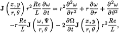 (8)
(8)
with a stream function defined by
where ![]() and
and ![]() are the Jacobians.
are the Jacobians.
In order to generate the computational domain, the classical Joukowski transformation is used. Additional stretching near the the foil surface impoves the resolution at the boundary layer region. The O-grid in the physical domain is ilustrated in Fig.2. On

Fig. 2: O-grid system—physical domain
the surface , the constraint of no slip is applied to define the surface vorticity. At the downstream boundary, the flow is assumed to be governed with first order differential relations obtained from the tangential NS eqs. by dropping the viscous term. For the upstream condition, the uniform velocity is assumed. Both vorticity and stream function eqs. are subjected to periodicity in θ-direction.
The vorticity equations is solved by an implicit factored method. The truncation error has the order of O[(Δr)2+(Δθ)4+(Δt)2], where Δr, Δθ and Δt are the space and time increments respectively. The Fourier transform method is used to solve the stream function equation by a direct approach. The vorticity and stream function equations are solved sequentially. The step is repeated until the convergence of surface vorticity is reached.
The surface pressure distribution is obtained by integrating the tangential component of NS eqs. For further details one may refer to the paper of Mehta [14] and [16].
Nondimensional coefficients are defined in the inertial frame as:
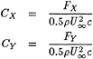
(10)
where, FX and FY are the forces acting on the foil in x0 and y0 direction (Fig.1) and M is the moment with respect to the pivot point location.
The hydrodynamical efficiency of propulsion of the motion is defined as:
The path of the pivot point is described by the relations
(11)
where ![]() and
and ![]() are normalized surging and heaving velocities. Thrust force T and thrust coefficient CT is defined as the force and the coefficient acting into the direction of propulsion (negative X axis in this case) and will coincide with the drag force FX and drag coefficient CX. In such case, the work WT done by the thrust is
are normalized surging and heaving velocities. Thrust force T and thrust coefficient CT is defined as the force and the coefficient acting into the direction of propulsion (negative X axis in this case) and will coincide with the drag force FX and drag coefficient CX. In such case, the work WT done by the thrust is

(12)
where ![]() is the time for a cycle of oscillation. The power consumed by the torque force Q ≡ FY is
is the time for a cycle of oscillation. The power consumed by the torque force Q ≡ FY is
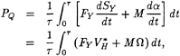 (13)
(13)
Then, the hydrodynamical efficiency of propulsion is :

(14)
where Ω* is normalized piching velocity and ![]() is at least one period of oscillation.
is at least one period of oscillation.
PILOT COMPUTATIONS
For the discussions on the real physical phenomena, it is necessary to examine the numerical accuracy. The following items should be studied; 1) time increment, 2) grid resolution and 3) parameters involved in the numerical procedure such as dissipative term, relaxation parameters, required accuracy for the surface vorticity convergence, minimum number of iterations for solving stream function-vorticity equations, etc. Although the quality of solution will depends on the flow complexity, we carry out this study through pilot computations.
Computational Parameters
(1) The effect of the time increment on the hydrodynamic loads was studied for several cases with different complexity[16]. Typical results are shown in Fig. 3 where a), b) and c) are the results by Δt, 4Δt and 10Δt respectively. In a), the time increment is chosen properly corresponding to the flow complexity, but its refinement does not lead to any significant improvements of the quality of solution as seen in b). A further increase leads to an intensive oscillation around the mean value; c). Sometimes, it leads to a lack of convergence at all. During the present computations the time increment varies from case to case with respect to the physical parameters and flow complexity. The know-how obtained at the initial stages of the study results to a time adaptive procedure which is capable to increase (to the safe limit of Δt*≤0.01) each 20 time steps or decrease the time increment automatically by factor of two if necessary.
(2) The grid resolution effects have been Fig. 3: The effect of the time increment on studied for the two grid systems; (66×42) and (130×84). An illustration of the influence of spatial resolution on flow pattern of a pitching foil is found in Fig. 4. The simulated flows by the two grid systems are qualitatively identical, although qualitative discrepancies are observed around the leading and trailing edges. The coarse grid system
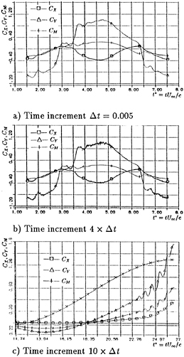
Fig. 3: The effect of the time increment on the solution

Fig. 4: Vorticity contours by two grid resolution ![]()
led to higher oscillations in force and slowed down the speed of convergence. Coarse grids cannot resolve small flow structures and gradients of the flow parameters with sufficient accuracy. It was seen that the grid resolution affects not only the pattern of the vorticity structures but also their intensity. Although further grid refinement is desirable, the second grid system of (130×84) can be concluded to be acceptable for the further discussions.
(3) The influence of other numerical parameters such as the number of iterations for the sequential solving of vorticity and stream function equations, the factors of the dissipative terms, and relaxation procedure, etc. have been studied. It was concluded that they are of secondary importance in comparison with the parameters already discussed. Special attention have to be payed to the criterion for convergence of the solution for the surface vorticity which is in direct connection with the physical parameters, time increment and grid resolution. Their combined effects may lead to an undesirable oscillation of the solution. More detailed analysis and a study of the influence of round-off errors performed indirectly comparing single and double precision results may be found in the written discussions of [16].
Physical Parameters
As it has been pointed out, the validity of the numerical solution is dependent heavily on the main physical parameters governing the flow phenomena. The most primary parameter is the Reynolds number based on the chord length. For the present computations this limiting value was estimated to be about Re≈1.0×10⁴. In our case, however, it seems to be more proper to define an effective Reynolds number as
where ![]() and
and ![]() are normalized velocities resulting from the foil motion. This parameter accounts to some extent for the flow complexity in combination with the effective incidence angle αeff.
are normalized velocities resulting from the foil motion. This parameter accounts to some extent for the flow complexity in combination with the effective incidence angle αeff.
For high frequency and large amplitude oscillations (or very distant pivot point locations), it appears that we can not proceed with the computations regardless how fine the time step is. For a bit smaller values of parameters of the foil motion, high frequency oscillations in the vorticity field are observed around the leading and trailing edges of the foil. An example is presented in Fig. 5 for the case with the reduced frequency of 1.0 and the pivot point located five chord lengths ahead the leading edge. The observed high frequency oscillations have rather numerical nature, although they are induced by physical reasons. Comments on similar results may be found in [14]. Our opinion is that the spectral method used combined with insufficient grid resolution can not handle with

Fig. 5: Vorticity contours at the trailing edge ![]()
high gradients of the flow with sufficient accuracy. How this oscillation will evolve further depends mainly on the current stage of the foil motion. If their appearance is taking place relatively early in the cycle, they may destroy the solution.
Pilot Computations and Comparison with Experimental Flow Visualization
Accuracy evaluation may be performed by comparing the numerical results with other published results or available experimental data. Here a comparison is made with the experimental data obtained in the frames of the present study. Fig. 6 shows one example of the comparisons; the particle path (for the time of exposition) and the contour lines of the stream function in the inertial frame of reference in which the experimental data were taken. The details about the experimental conditions may be found in [16]. The foil is pitching symmetrically with k=1.0, αA= 15º and ![]() . Reynolds number for the computations and experiment are both 0.5 ×10⁴. The experimental data were taken after the foil had performed several cycles of oscillations. The main flow structures observed in the experiment are well predicted numerically. Observed differences are in the range of uncertainty of experiments.
. Reynolds number for the computations and experiment are both 0.5 ×10⁴. The experimental data were taken after the foil had performed several cycles of oscillations. The main flow structures observed in the experiment are well predicted numerically. Observed differences are in the range of uncertainty of experiments.
All the discussed results seem to indicate that the present numerical study is of sufficient accuracy to allow a physical interpretation of computational data.
HEAVING MOTION
Basic Flow Features
The flow evolution for a typical heaving motion is presented in Fig. 7, showing the streamlines in a frame attached to the foil at some selected stages during the two cycles of heaving motion. The foil is heaving according to eq.(1) with a reduced frequency kh of 0.52 and normalized amplitude ![]() . All the results shown hereafter concern fully developed flows after the foil is accelerated to the required Reynolds number of 0.5×10 4. This stage serves as initial conditions for the consequent phase of harmonic oscillations with the prescribed governing parameters.
. All the results shown hereafter concern fully developed flows after the foil is accelerated to the required Reynolds number of 0.5×10 4. This stage serves as initial conditions for the consequent phase of harmonic oscillations with the prescribed governing parameters.
Initially, the flow is undisturbed and slightly separated at the trailing edge . At the next stage (in the present case the foil starts to move downward), the separation over the upper side of foil propagates upstream, while the front stagnation point rolls down (Fig.7 a)). Leading edge separation appears long after the effective incidence angle (αeff) exceeded the static stall limits. This phase is illustrated in Fig. 7 b). αeff at this moment is about 30º. After the foil passed the zero level, the heaving velocity decelerates and the effective incidence angle also decreases. At this stage, the flow is fully separated. As the foil decelerates further, the leading edge vortices are convected faster (Fig. 7 c), d)). In the second cycle, the vortices are shed into the wake and the flow differs in detail from the first cycle, although the general behavior shown in Fig. 7 d) is similar to Fig. 7 a). The formation of the leading edge vortex is postponed in the second cycle. This later formation leads to moderate intensity and faster convection
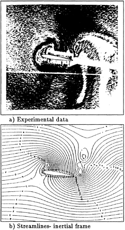
Fig. 6: Flow visualization and numerical data ![]()
of vortices into downstream (Fig. 7 e)). After two cycles, in Fig. 7 f), the flow pattern is similar to that of c) with some differences caused by the wake influence.
Fig. 8, the surface pressure distribution. As can be seen, the pressure is affected mainly by the leading edge vortex and its propagation over the foil surface and wake formation. A sharp suction peak observed at early stage is smoothened as the separation appear. The peak of the leading edge vortex travels along the chord into downstream. Its magnitude corresponds to the vortex intensity. The time history of the drag, lift and moment coefficients is presented in Fig.9. The dynamic changes in the induced forces follow the respective changes in the flow pat tern and the pressure distribution. Negative drag means that a propulsive force is realized.
Parametric Study
In order to investigate the effect of acceleration, two cases are studied. They have the same effective incidence angle as a “standard ” one, but the acceleration is twice larger or smaller; the first one has parameters k=0.26, hA=1.2; for the second one k=1.04, hA=0.3.
Flow patterns of these two cases are shown in Fig. 10 and Fig. 11. They may be compared with the results for the ”standard heaving” case presented in Fig. 7 b),c) and e). Small foil acceleration can not delay the leading edge separation. The stall vortex is well developed when for the case of large acceleration, the leading edge separation just starts with a short bubble (see Figs. 10 a) and 11 a)). In the case of small k, it has much lower intensity than in the case of large frequences, but its diffusion covers a large area. Small inertial effects allow its detachment from the foil surface. The process of light stall in case of small k is illustrated in Fig.10 c). Strong flow separation at this stages leads to a large drag coefficient and low overall propulsive efficiency. Even at the same effective incidence, the flow is much smoother in case of large k
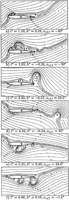

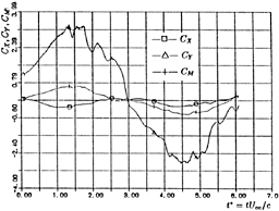
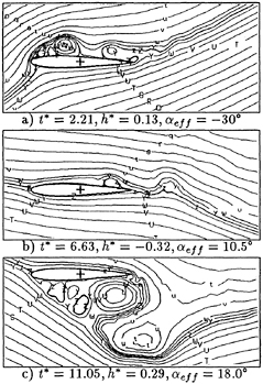
Fig.10: Streamlines in a moving frame (![]() =1.2, k=0.26; small acceleration)
=1.2, k=0.26; small acceleration)
(Fig. 11 c)). The leading edge vortex formed during the downstroke is finally shed and improves the circulation around the foil to cause a better propulsion.
Performance
Fig. 12 and Fig. 13 present the drag, lift and moment coefficients for the discussed cases. The thrust force for the k=1.04 (Fig. 13) is larger than that of the k=0.26 (Fig. 12) and slightly larger than the ”standard” one (Fig. 9). The realized efficiency, η=0.16, is comparable with that of the standard case (η=0.10).
Small increase of the reduced frequency leads to slight improvement in the efficiency. In the cases of very high reduced frequency with small amplitude of oscillations, the efficiency drops rapidly as the thrust/lift ratio
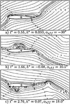
Fig. 11: Streamlines in a moving frame (![]() = 0.3, k=1.04; large acceleration)
= 0.3, k=1.04; large acceleration)
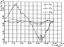
Fig.12: History of drag (CX), lift (CY) and moment (CM) coefficient (![]() =1.2, k= 0.26)
=1.2, k= 0.26)
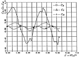
Fig. 13: Drag (CX), lift (CY) and moment (CM) coefficient (![]() =0.3 k=1.04)
=0.3 k=1.04)

Fig. 14: Drag (CX), lift (CY) and moment (CM) coefficient (![]() =0.018, k=7.78)
=0.018, k=7.78)
decreases. The coefficients of the hydrodynamic loads for the case of k=7.78 and ![]() =0.018 are presented in Fig. 14. Because the inertial terms are large in this case, the viscous effect is reduced and there is no evidence of separation. The lift is completely out of phase which corresponds qualitatively to the result of Choi and Landweber [15]. However, the results differ quantitatively from those obtained by the potential flow methods. This is because the assumption of the Kutta condition is strongly violated.
=0.018 are presented in Fig. 14. Because the inertial terms are large in this case, the viscous effect is reduced and there is no evidence of separation. The lift is completely out of phase which corresponds qualitatively to the result of Choi and Landweber [15]. However, the results differ quantitatively from those obtained by the potential flow methods. This is because the assumption of the Kutta condition is strongly violated.
Potential methods predict that the efficiency will decrease with the increase of reduced frequency (see for example Katz[17]). The results shown in Fig. 12 and Fig. 13 lead to the just opposite conclusion. The main reason is that the higher frequency decrease leading edge separation which is not included in potential schemes. When the reduced frequency is low and amplitude large, the flow is characterized by a strong leading edge separation at the early stages of heaving. Such result is caused by weak unsteady effects. This separation has strong impact on the wake and the resulted circulation. It leads to a large drag and low efficiency.
The principal result is that pure having motion may produce a propulsive force but the efficiency is low.
PITCHING MOTION
The pitching motion is performed symmetrically according to the eq.3. The reduced frequency k, angular amplitude αA and normalized pivot point location ![]() can be the parameters of motion.
can be the parameters of motion.
Cases when the pivot point is located far ahead or far behind the foil were studied in [16]. In these cases, the foil produces thrust but small in mean value. Fig. 15 shows a typical example of the time history of the force coefficients; the pivot point is located between the leading edge and the middle of the foil chord. When the foil is pitching around an axis located near the middle of the chord, it can not produce a propulsive force.
Fig. 16 shows one of the flow patterns, when the pivot point is located at the leading edge of the foil. In this case, leading edge separation is prevented almost completely. However, large trailing edge separation is generated which induces an increase of the drag.
Comparing with the heaving motion, it is revealed that acceleration of the foil is responsible for the unsteady effects. In the
pitching case, the acceleration is expressed by k2![]() αA, so that the flow near the trailing edge is highly dependent on the reduced frequency and the distance to the pivot point location. It is found out that the flow changes dramatically when the pivot point is located relatively near and ahead of the leading edge.
αA, so that the flow near the trailing edge is highly dependent on the reduced frequency and the distance to the pivot point location. It is found out that the flow changes dramatically when the pivot point is located relatively near and ahead of the leading edge.

Fig. 17: Streamlines in a moving frame (![]() = 0.0, k=3.0, αA=15º t*=1.05)
= 0.0, k=3.0, αA=15º t*=1.05)
When the oscillations are of relatively low frequency, the trailing edge separation is large to lead to a large drag force. As the frequency of oscillations increases, the inertial terms play a more significant role. Trailing edge separation decreases rapidly when the leading edge separation is negligible (Fig. 17). Wake development assists production of a propulsive force and relatively large forward thrust may be obtained. Time variations of the coefficients for this case are presented in Fig. 18. The shift in phase of the lift improves additionally the efficiency (η=0.23).
Further improvement of propulsive abilities was reached when the pivot point location was moved ahead to the leading edge by a half chord. The flow pattern is illustrated in Fig. 19. Although small but intensified separation vortices are observed around the leading edge, quite high efficiency of 0.62 is realized for this case. The coefficients of

Fig. 15: Drug (CL), lift (CD) and moment (CM) coefficients (![]() = 0.1, k = 0.5, αA = 15º)
= 0.1, k = 0.5, αA = 15º)

Fig. 16: Streamlines in a moving frame ( ![]() = 0.0 k = 1.5, αA = 15º, t* = 1.05)
= 0.0 k = 1.5, αA = 15º, t* = 1.05)

Fig.18: Drag (CX), lift (CY) and moment (CM) coefficients (![]() =0.0, k=3.0, αA= 15º)
=0.0, k=3.0, αA= 15º)
induced forces are shown in Fig. 20. The combined effects of lift phasing, large suction at the leading edge, wake interaction and energy extraction from the near wake results in such higher efficiency. The present result may suggest how the pure pitching motion could be efficiently propulsive.
COMBINED MOTION
The case of combined motion is that heaving, pitching and surging motions are combined.
The ”standard case” has the same reduced frequency and heaving amplitude as the standard heaving case (k=0.52, hA= 0.6). Pitching is performed around a pivot point located at 0.25c from leading edge with the amplitude of 20º. The effective incidence angle at the pivot point location is ranging in [−15º, 15º] during one cycle. Such motion may lead to an efficient propulsive force as strong separation can not be expected.
Fig. 21 shows the flow pattern at the selected stages, visualized by the stream function contours in a moving frame fixed to the foil. Soon after the motion has begun, very small separation bubble formed earlier near the leading edge and a weak trailing edge sep

Fig. 19: Streamlines in a moving frame ( ![]() = –0.5 k = 3.0 αA = 15º, t* = 1.45)
= –0.5 k = 3.0 αA = 15º, t* = 1.45)
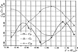
Fig. 20: Drag (CX), lift (CY) and moment (CM) coefficients (![]() =−0.5, k=3.0, αA= 15º)
=−0.5, k=3.0, αA= 15º)
aration are observed (Fig. 21 a)). Stronger separations have been prevented by the foil acceleration at the initial stage. At the moment shown in Fig. 21 a) the foil already decelerates and separation of the boundary layer grows. The trailing edge vortex is shed when the bubble separates in two smaller structures which travel into downstream over the foil.
Fig. 21 b) illustrates the flow, when the foil is at the maximum amplitude and starts its motion downward. Separation is stronger on the lower side. At the following stage, the separation vortices are washed into downstream (Fig. 21 c)). A developed wake leads to delay of the flow evolution in comparison with the initial stage (Fig. 21 a)) but does not prevent the flow separation when the foil is altering the direction of the heaving motion again (Fig. 21 d)).
Such flow behavior is common and is repeated in the following cycles. Comparing with the result for the pure heaving and the pure pitching cases, the unsteady effects and wake interaction are less.
Fig. 22 shows the pressure distribution on the foil. The wavy peak of pressure is caused by the leading edge vortex and its propagation in time. Fig. 23 shows the time histories of drag, lift and moment coefficients. Qualitatively and in average, the behavior of the induced forces is comparable with the predictions made by the potential model (see for example [17]).
However, they differ in details. Separation of the boundary layer at the stages when the foil is about turning position is causing larger drag and loss of efficiency. It seems that viscous effects are considerable for the flows whose Reynolds number is around 0.5 ×10⁴.
Parametric Study and Performance
Parametric studies are carried out by changing the frequency k, the amplitude heaving and pitching hA, αA, and the position of pitching axis ![]() (Table1). C0 is the standard case.
(Table1). C0 is the standard case.

Fig. 21: Streamlines in a moving frame (![]() =0.6, k=0.52, αA=20º)
=0.6, k=0.52, αA=20º)

Fig. 22: Surface pressure coefficient −CP (![]() =0.6, k=0.52, αA= 20º)
=0.6, k=0.52, αA= 20º)

Fig. 23: Drag (CX), lift (CY) and moment (CM) coefficient (![]() =0.6, k=0.52, αA= 20º)
=0.6, k=0.52, αA= 20º)
Table 1: Cases for the parametric studies of combined motion.
|
Case |
k |
hA |
αA |
|
η |
|
C0 |
0.52 |
0.6 |
20º |
0.25 |
0.47 |
|
C1 |
0.26 |
1.2 |
20º |
0.25 |
0.51 |
|
C2 |
1.04 |
0.3 |
20º |
0.25 |
0.41 |
|
C3 |
0.52 |
0.6 |
20º |
0.00 |
0.55 |
|
C4 |
0.52 |
0.6 |
20º |
0.50 |
0.48 |
|
C5 |
0.52 |
1.2 |
40º |
0.25 |
0.61 |
|
C6 |
0.52 |
2.4 |
60º |
0.25 |
0.55 |
The effects of the reduced frequency and the heaving amplitude are studied by the cases C1 and C2. The effective incidence angle for these two cases is the same as the standard case. In case C1, the leading edge separation appears earlier due to the smaller dynamic effects. It covers a larger domain (Fig.24 a)) comparing with the standard case. The magnitude of induced forces is bigger as no stall effect is observed. When the foil is altering its direction of heaving, the energy of the shedding vortices is partially extracted back as shown in Fig.24 a). All these facts result in an improvement of efficiency (refer Table.1).
In the case C2 where the acceleration and deceleration is high, the dynamic effects are stronger. The phase of acceleration delays leading edge separation much longer Fig.24 b). At the same time the trailing edge separation is more intensive to cause a worse performance.
The dependency on the pivot point location is investigated by the cases C3 and C4. In the case C3 where the pivot point is at the leading edge, the leading edge separation is prevented (Fig.24 c)). In the case C4 an opposite tendency is observed as shown in Fig.24 d). The leading edge separation appears earlier due to the larger angular deceleration of the leading edge. Its reattachment leads to a trailing edge vortex. When the foil approaches the position of the maximum amplitude, the case of C4 has a worse efficiency.
After the turn, the flow near the leading edge is accelerated, so that the disturbances are washed easier and the foil starts to produce thrust earlier than the other cases. Such a compensation results in a similar efficiency compared with the standard case.
The effect of pitching and heaving amplitude is studied in the case C5. Larger amplitude of heaving combined with larger pitching amplitude may be more efficient. The main reason is that the foil inclination compensates the increase of the effective incidence angle to make the thrust component of the reaction force larger. If the energy losses are not so large during the turn, a better efficiency could be obtained. Leading edge separation appears earlier and forms a series of vortices (Fig. 24 e)). The mean value of the ratio CX/CY is very high. When the foil approaches its heaving amplitude, the separation grows considerably. The shedding of the edge vortices leads to an energy extraction. However, much larger amplitude fails to increase the efficiency as seen in the case C6. The separation is much more intensive and remain longer after the foil is altering the direction of heaving. It causes a large drag force. This fact leads to a worse efficiency.
GENERAL DISCUSSION
Parametric studies described in the previous sections indicate that flow phenomena depend much more on the parameters of the motion than on the type of motion itself such as heaving, pitching and surging. Driving parameters have a complicated and interrelated influence on the flow pattern and induced forces. In the light of obtained results, conclusions like ”as the reduced frequency increases, the mean thrust increases while the efficiency decreases.” seem to be ambiguous. It could be true or could not be as it depends on the other parameters and all complexity of dynamic effects. For example, the resultant effective angle of attack, strong trailing and leading edge separation and stall depend much on the parameters. When driv-

Fig. 24: Parametric study of combined motion. Streamlines for the middle of the second cycle
ing parameters postulate a foil motion with significant foil acceleration and deceleration, strong unsteady dynamic effects govern the flow evolution. When the foil is accelerating, leading edge separation is prevented or postponed. If a separation appears at this stage, it produces intensive vortical structures which evolve rather by diffusion than by convection. On the other hand, the deceleration assists separation process. Quite different flow phenomena are observed for the cases characterized by small amplitude oscillations with extremely high reduced frequency Strong inertial forces govern the flow pattern overwhelming viscous effects. They will dump transition and turbulent effects as well.
From this point of view, the results obtained by a potential method may be questioned even qualitatively. Obviously, such methods will provide unrealistic results and misleading conclusions for strong unsteady viscous effects as studied.
The Reynolds number may affect the results not only quantitatively but qualitatively as well. Its effect is studied for the combined motion (case C0). Computations were carried out for Re=1.0×10³ and Re=1.0×10⁴, including Re=0.5×10⁴ for the case C0. Its influence on the flow pattern is illustrated in Fig. 25 as in Fig. 21 d) for the standard case. It is well seen that the effect is not negligible even within this small variation. In the case of Re=1.0×10³, the leading edge separation vanishes but the trailing edge separation is much stronger. For Re=1.0×10⁴ the leading edge separation is stronger, but the scale is smaller and more intensive. The flow reat-taches faster. Such qualitative differences are valid all the way during the motion. As a result a better efficiency (η=0.54) is realized at higher Reynolds number. In the case of low Reynolds number the efficiency dropped to η=0.30.
The time histories of force coefficients are shown in Fig. 26 a) and b) for Re= 1.0×10³ and Re=1.0×10⁴. the low and high Re respectively. Comparing efficiency

Fig. 25: Effect of Reynolds number on the flow pattern (![]() =0.6, k=0.52, αA=20º)
=0.6, k=0.52, αA=20º)
coefficients for the three Reynolds numbers we may suggest that at really high Reynolds numbers the propulsion may be of considerable for the practice efficiency.
Except the cases of pitching with high frequency around a pivot point in front of the leading edge, the only motion with considerable high efficiency is the combined one. The efficiency is very sensitive to the variations of parameters. An extensive research is needed to specify in details the best combination of parameters for a more efficient propulsion system.
CONCLUSION
Numerical simulation of viscous unsteady flow around an oscillating 2D hydrofoil is performed. An implicit finite difference method is implemented. Main flow features and its dependency to the foil motion are investigated. Obtained results lead to the following main conclusions:
-
Pilot computations and comparison of the numerical results with available experimental data concluded that the ba
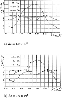
Fig. 26: Effect of the Reynolds number on the indiced forces ( ![]() =0.6, k=0.52, αA= 20º)
=0.6, k=0.52, αA= 20º)
-
sic flow features are modeled with sufficient accuracy to merit physical analysis. However, the accuracy simulations may be limited with respect to the used grid resolution.
-
Basic flow features depend strongly on the main parameters governing the foil motion. The parametric study indicated their interrelated influence. The foil acceleration is revealed as a major physical parameter for the unsteady and viscous effects.
-
The ability of an oscillating foil to produce forward thrust is in direct connection with the foil motion and resulted flow. Pure heaving motion can produce thrust but of limited efficiency. This conclusion is valid for the pitching motion, except the cases of very high frequency and the pivot point located slightly ahead of the leading edge of the foil.
-
Combined foil motion can produce thrust force with high efficiency. Simulated results show the complicated nature of thrust production and the heavy dependence of the efficiency on the parameters of the motion. Further investigations may be needed for tuning these parameters if efficiency has to be improved.
-
Complicated flow phenomena lead to the conclusion that 3D effects as well as turbulent effects may play an important role.
References
[1] McCroskey, W.J., ”Unsteady Airfoils,” Annual Review of Fluid Mechanics, 1982, pp. 285–311.
[2] Carr, L.W., ”Dynamic Stall Progress in Analysies and Prediction,” AIAA Paper 85–1769CP, 1985.
[3] Lighthill, M.J., ”Note on the swimming of slender fish,” Journal Fluid Mechanics, Vol. 9, 1960, pp. 305–317.
[4] Wu, T.Y., ”Swimming of waving plate,” Journal Fluid Mechanics, Vol. 10, 1961, pp. 321–344.
[5] Lighthill, M.J., ”Biofluiddynamics of balistiform and gymnotiform locomotion. Part 2. The pressure distribution arising in two-dimensional irrotational flow from a general symmetrical motion of a flexible flat plate normal to itself,” Journal Fluid Mechanics, Vol. 213, 1990, pp. 1–10.
[6] Karpouzian, G., Spedding, G. and Cheng, H.K., ”Lunate—tail swimming propulsion. Part 2. Performance analysis,” Journal Fluid Mechanics, Vol. 210, 1990, pp. 329–351.
[7] Chopra, M.G., ”Hydromechanics of lunate—tail swimming propulsion,” Journal Fluid Mechanics, Vol. 64, 1974, pp. 375–391.
[8] Chopra, M.G., ”Large amplitude lunate— tail theory of fish locomotion,” Journal Fluid Mechanics, Vol. 74, 1976, pp. 161– 182.
[9] Chopra, M.G., ”Hydromechanics of lunate—tail swimming propulsion. Part 2,” Journal Fluid Mechanics, Vol. 79, 1977, pp. 49–69.
[10] Lan, C.E., ”The unsteady quasi—vortex—lattice method with applications to animal propulsion,” Journal Fluid Mechanics, Vol. 93, Part 4, 1979, pp. 749–765.
[11] Cheng, J.Y., Zhuang, L.X., Tong, B.G., ”Analysis of swimming three—dimensional waving plates,” Journal Fluid Mechanics, Vol. 232, 1991, pp. 341–355.
[12] Kudo, T., Kubota, A., Kato, H., Yamaguchi, H., ”Study on Propulsion by Partially Elastic Oscillatinf Foil. 1st Report. Analysis by Linearized Theory,” J. Soc. Naval Arch. of Japan, Vol. 156, Nov. 1984, pp. 82–91. (in Japanese).
[13] Kubota, A., Kudo, T., Kato, H., Yamaguchi, H., ”Study on Propulsion by Partially Elastic Oscillatinf Foil. 2nd Report. Numerical simulation by singularity distribution method and evaluation of scope for application to ship propulsion,” J. Soc. Naval Arch. of Japan, Vol. 156, Nov. 1984, pp. 82–91. (in Japanese)
[14] Mehta, U.B., ”Dynamic Stall of an Oscillating Airfoil,” AGARD Paper 23, Unsteady Aerodynamics, AGARD CP-227, Sept. 1977.
[15] Choi, D.H., Landweber, L., ”Inviscid Analysis of Two-Dimensional Airfoils in Unsteady Motion Using Conformal Mapping,” AIAA Journal, Vol. 28, No. 12, Dec.1990, pp. 2025–2033.
[16] Videv, T.A. and Doi, Y., ”Numerical Study of the Flow and Thrust Produced by a Pitching 2D Hydrofoil,” J. Soc. Naval Arch. of Japan, Vol. 172, Nov. 1992, pp. 165–174.
[17] Katz, J. and Weihs, D., ”Hydrodynamic propulsion by large amplitude oscillation of an airfoil with chordwise flexibility,” Journal Fluid Mechanics, Vol. 88, Part 3, 1978, pp. 485–497.


