
A Fast Multigrid Method for Solving the Nonlinear Ship Wave Problem with a Free Surface
J.Farmer, L.Martinelli, and A.Jameson
(Princeton University, USA)
Abstract
This paper presents a finite volume method for the solution of the three dimensional, nonlinear ship wave problem. The method can be used to obtain both Euler and Navier-Stokes solutions of the flow field and the a priori unknown free surface location by coupling the free surface kinematic and dynamic equations with the equations of motion for the bulk flow. The evolution of the free surface boundary condition is linked to the evolution of the bulk flow via a novel iteration strategy that allows temporary leakage of mass through the surface before the solution is converged. The method of artificial compressibility is used to enforce the incompressibility constraint for the bulk flow. A multigrid algorithm is used to accelerate convergence to a steady state. The two-layer eddy viscosity formulation of Baldwin and Lomax is used to model turbulence. The scheme is validated by comparing the numerical results with experimental results for the Wigley parabolic hull and the Series 60, Cb=0.6 hull. Waterline profiles from bow to stern are in excellent agreement with experiment. The computed wave drag compares favorably with experiment. Overall, the present method proves to be accurate and efficient.
1
Introduction
It is well established that a complex interaction exists between the viscous boundary layer and wake of a ship hull and the resulting wave pattern [1, 2]. The existence of two similarity parameters, the Froude number (Fr) and the Reynolds number (Re), which do not scale identically between model and full scale hulls, make it difficult to predict the viscous effect on the wave and total drag through model testing. The ship designer may thus resort to numerical simulation, and a great deal of effort has been devoted toward developing numerical tools capable of simulating the flow field about a translating ship. Some of these tools have met with success in capturing the salient features of the flow field, including the difficult-to-model stern region of ship hulls. However, many of the computational methods developed to date, especially those that include viscous effects and a moving free surface, tend to be very complicated and expensive. Thus, the focus of this work is the development of a fast and robust means to compute either viscous or inviscid flow fields about surface piercing ship hulls, and to make comparisons with experimental data.
The method of Hino [3] is a widely used approach for solving incompressible flow problems. This method takes the divergence of the momentum equation and solves implicit equations at each time step for the pressure and velocity fields such that continuity is satisfied. The method is expensive both because of the need to solve implicit equations by an iterative method and because of the cost of calculating the divergence of the momentum equations in a curvilinear coordinate system. Hino uses a finite difference scheme expressed in body-fitted curvilinear coordinates to discretize the solution domain on and below the free surface. The computational grid is not allowed to move with the free surface so an approximation must be employed to model the free surface boundary conditions. A Baldwin-Lomax turbulence model is used in conjunction with the wall function to model the viscous boundary layer. The scheme is first-order accurate in time and requires 104-plus global iterations to reach steady state for simple hull shapes.
The method of Miyata et al. (1987) [4] uses a similar velocity and pressure coupling procedure but now the grid is allowed to move with the free surface, providing a more exact treatment of the free surface boundary conditions. A sub-grid-scale turbulence model is employed and computations performed for Reynolds numbers up to 105. As with Hino's method, the time-accurate formulation necessitates several thousand time steps to reach steady state solutions. In a later paper, Miyata et al. (1992) [5] present a finite volume approach that substantially improves the computed results over those obtained using the finite difference approach. Simulations using Reynolds numbers up to 106 were made and more complicated hull shapes examined. The method still requires many thousands of time steps to achieve steady state solutions.
The interactive approach of Tahara et al. [6] uses a field method based on the finite-analytic method used by Chen et al. [7] for the viscous region, and a surface singularity method based on the “SPLASH” panel method of Rosen [8] for the inviscid outer domain. The method iterates between the inviscid and viscous regions by adjusting the small-domain panel distribution to allow for the boundary layer displacement thickness determined from the large-domain solution. The free surface boundary conditions are linearized and applied at the mean water elevation surface. Results of this approach appear to be quite promising for the Wigley hull, and a substantial savings in required computational cost is realized over the large-domain approaches of Hino and Miyata.
In this work, a field method is adopted for the entire flow domain like Hino and Miyata. However, the incompressibility constraint is enforced through the method of artificial compressibility, rather than the velocity-pressure coupling method. The method of artificial compressibility was originally proposed by Chorin [9] in 1967 to solve viscous flows. Since then, Rizzi and Eriksson [10] have applied it to rotational inviscid flow, Dreyer [11] has applied it to low speed two dimensional airfoils and Kodama [12] has applied it to ship hull forms with a symmetric free surface. In addition, Turkel [13] has investigated more sophisticated preconditioners than those originally proposed by Chorin. The basic idea behind artificial compressibility is to introduce a pseudotemporal equation for the pressure through the continuity equation. Use of this pressure equation, rather than the velocity-pressure coupling procedure described in references [3]—[7], renders the new set of equations well conditioned for numerical computation along the same lines as those used to calculate compressible flow about complete aircraft [14,15]. When combined with multigrid acceleration procedures [16,17,18] it proves to be particularly effective. Converged solutions of incompressible flows over three dimensional isolated wings are obtained in 25–50 cycles.
The general objective of this work is to build on these ideas to develop a more efficient method to predict free surface wave phenomena, for both inviscid and viscous flows. The viscous solution method introduced in this work is an extension of the inviscid method presented in reference [19, 20]. The nonlinear free surface boundary condition is satisfied by an iterative procedure in which the grid is moved with the free surface. Comparisons of numerical predictions with experimental data, for the Wigley hull and Series 60, Cb=0.6 ship hull, show encouraging results for both waterline profiles and wave drag. Furthermore, it appears that this approach yields a substantial savings in the computational resources required for the simulations.
2
Mathematical Model
Figure 1 shows the reference frame and ship location used in this work. A right-handed coordinate system Oxyz, with the origin fixed at midship on the mean free surface is established. The z direction is positive upwards, y is positive towards the starboard side and x is positive in the aft direction. The free stream velocity vector is parallel to the x axis and points in the same direction. The ship hull pierces the uniform flow and is held fixed in place, ie. the ship is not allowed to sink (translate in z direction) or trim (rotate in x–z plane).
2.1
Bulk Flow
For a viscous incompressible fluid moving under the influence of gravity, the continuity equation and the Reynolds averaged Navier-Stokes equations may be put in the form [3],
ux+νy+wz=0 (1)
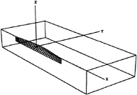
Figure 1: Reference Frame and Ship Location
νt+uνx+ννy+wνz= −ψy+(Re−1+νt) (▽2ν) (2)
wt+uwx+vwy+wwz= −ψz+(Re−1+νt) (▽2w).
Here, u=u(x,y,z,t), ν=ν(x,y,z,t) and w=w(x,y,z,t) are the mean total velocity components in the x,y and z directions. All lengths and velocities are nondimensionalized by the ship length L and the free stream velocity U, respectively. The pressure ψ is the static pressure p minus the hydrostatic component −zFr−2 and may be expressed as ψ=p+zFr−2, where ![]() is the Froude number. The pressure variable ψ is nondimensionalized by ρU2. The Reynolds number Re is defined by
is the Froude number. The pressure variable ψ is nondimensionalized by ρU2. The Reynolds number Re is defined by ![]() where ν is the kinematic viscosity of water and is constant. νt is the dimensionless turbulent eddy viscosity, computed locally using the Baldwin-Lomax turbulence model. This set of equations shall be solved subject to the following boundary conditions.
where ν is the kinematic viscosity of water and is constant. νt is the dimensionless turbulent eddy viscosity, computed locally using the Baldwin-Lomax turbulence model. This set of equations shall be solved subject to the following boundary conditions.
2.2
Boundary Conditions
2.2.1
Free Surface
When the effects of surface tension and viscosity are neglected, the boundary condition on the free surface consists of two equations. The first, the dynamic condition, states that the pressure acting on the free surface is constant. The second, the kinematic condition, states that the free surface is a material surface: once a fluid particle is on the free surface, it forever remains on the surface. The dynamic and kinematic boundary conditions may be expressed as
p=constant
(3)
where z=β(x,y,t) is the free surface location. Equation 3 only permits solutions where β is single valued. Consequently, it does not allow for the breaking of bow waves which can often be observed with cruiser type hulls. Breaking waves are difficult to treat numerically and are not considered in this work.
2.2.2
Hull and Farfield
The remaining boundaries consist of the ship hull, the boundaries which comprise the symmetry portions of the meridian plane and the far field of the computational domain. On the ship hull, the condition is that of no-slip and is stated simply by
u=ν=w=0.
On the symmetry plane (that portion of the (x,z) plane excluding the ship hull) derivatives in the y direction as well as the ν component of velocity are set to zero. The upstream plane has u=U and ψ=0 (p=−zFr−2) with the ν and w velocity components set to zero. Similar conditions hold on the bottom plane which is assumed to represent infinitely deep water where no disturbances are felt. One-sided differences are used to update the flow variables on the starboard plane. A radiation condition should be imposed on the outflow domain to allow the wave disturbance to pass out of the computational domain. Although fairly sophisticated formulations may be devised to represent the radiation condition, simple extrapolations proved to be sufficient in this work.
2.3
Turbulence Model
To model turbulence in the flow field the laminar viscosity is replaced by
μ=μl+μt
where the turbulent viscosity μt is computed using the algebraic model of Baldwin and Lomax [22]. The Baldwin-Lomax model is an algebraic scheme that makes use of a two-layer, isotropic eddy viscosity formulation. In this model the turbulent viscosity is evaluated using
where y is the distance measured normal to the body surface and ycrossover is the minimum value of y where both the inner and outer viscosities match. The inner viscosity follows the Prandtl-Van Driest formula,
where
l=ky[1−exp(−y+/A+)]
is the turbulent length scale for the inner region, k and A+ are model constants, |ω| is the vorticity magnitude and ![]() is the dimensionless distance to the wall in wall units.
is the dimensionless distance to the wall in wall units.
In the outer region of the boundary layer, the turbulent viscosity is given by
(μt)outer=KCcpFwakeFKleb
where K and Ccp are model constants, the function Fwake is
and the function FKleb is
![]() .
.
The quantities Fmax and ymax are determined by the value and corresponding location, respectively, of the maximum of the function
F=y|ω|[1−exp(−y+/A+)].
The quantity Udif is the difference between maximum and minimum velocity magnitudes in the profile and is expressed as
CKleb and Cwk are additional model constants. Numerical values for the model constants used in the computations are listed here:
A+=26, k=0.4, K=0.0168,
and
Ccp=1.6, Cwk=1.0, CKleb=0.3.
3
Numerical Solution
The formulation of the numerical solution procedure is based on a finite volume method (FVM) for the bulk flow variables (u,ν,w and ψ), coupled to a finite difference method for the free surface evolution variables (β and ψ). Alternative cell-centered and cell-vertex formulations may be used in finite volume schemes [16]. A cell-vertex formulation was preferred in this work because values of the flow variables are needed on the boundary to implement the free surface boundary condition. The bulk flow is solved subject to Dirichlet conditions for the free surface pressure, followed by a free surface update via the bulk flow solution (ie. constant values for the velocities in equation 3). Each formulation is explicit and uses local time stepping. Both multigrid and residual averaging techniques are used in the bulk flow to accelerate convergence.
3.1
Bulk Flow Solution
Following Chorin [9] and more recently Yang et al. [23], the gover ning set of incompressible flow equations may be written in vector form as
wt*+(f−fv)x+(g−gv)y+(h−hv)z=0 (4)
where the vector of dependent variables w and inviscid flux vectors f, g and h are given by

The viscous flux vectors fv, gv and hv are given by
 .
.
where the viscous stress components are defined as
 .
.
Г is called the “artificial compressibility” parameter due to the analogy that may be drawn between the above equations and the equations of
motion for a compressible fluid whose equation of state is given by [9]
ψ=Г2ρ.
Thus, ρ is an artificial density and Г may be referred to as an artificial sound speed. When the temporal derivatives tend to zero, the set of equations satisfy precisely the incompressible equations 2, with the consequence that the correct pressure may be established using the artificial compressibility formulation. The artificial compressibility parameter may be viewed as a device to create a well posed system of hyperbolic equations that are to be integrated to steady state along lines similar to the well established compressible flow FVM formulation [18]. In addition, the artificial compressibility parameter may be viewed as a relaxation parameter for the pressure iteration. Note that temporal derivatives are now denoted by t* to indicate pseudo time; the artificial compressibility, as formulated in the present work, destroys time accuracy.
To demonstrate the effect of Г on the above set of equations and to establish the hyperbolicity of the set, the convective part of equation 4 may be written in quasi-linear form to determine the eigenvalues [10]. The eigenvalues are found to be
λ1=U, λ2=U, λ3=U+a, λ4=U−a,
where
U=uωx +νωy+wωz
and
The wave number components ωx, ωy and ωz are defined on −∞≤ωx, ωy,ωz≤+∞. Since the eigenvalues are clearly real for any value of ωx, ωy and ωz, the system of equations 4 is hyperbolic.
The choice of Г is crucial in determining convergence and stability properties of the numerical scheme. Typically, the convergence rate of the scheme is dictated by the slowest system waves and the stability of the scheme by the fastest. In the limit of large Г the difference in wave speeds can be large. Although this situation would presumably lead to a more accurate solution through the “penalty effect” in the pressure equation, very small time steps would be required to ensure stability. Conversely, for small Г, the difference in the maximum and minimum wave speeds may be significantly reduced, but at the expense of accuracy. Thus a compromise between the two extremes is required. Following the work of Dreyer [11], the choice for Г is taken to be
Г2=γ(u2+v2+w2),
where γ is a constant of order unity. In regions of high velocity and low pressure where suction occurs, Г is large to improve accuracy, and in regions of lower velocity, Г is correspondingly reduced.
The choice of Г also influences the outflow boundary condition, or radiation condition. If it can be demonstrated that all system eigenvalues are both real and positive, then downstream or outflow boundary points may be extrapolated from the interior upstream flow. Even though an examination of the eigenvalues reveals that this can never be the case, the condition can be approached by a judicious choice of Г. If Г is large, extrapolation fails because the flow has both downstream and upstream dependence. As Г is reduced, the upstream dependence becomes more pronounced and the downstream is reduced. Eventually, the upstream dependence is sufficiently dominant to allow extrapolation. Hence, all outflow variables are updated using zero gradient extrapolation.
Following the general procedures for FVM, the governing equations may be integrated over an arbitrary volume Λ. Application of the divergence theorem on the convective and viscous flux term integrals yields

(5)
where Sx, Sy and Sz are the projected areas in the x, y and z directions, respectively. The computational domain is divided into hexahedral cells. Application of FVM to each of the computational cells results in the following system of ordinary differential equations,
The volume Λijk is given by the summation of the eight cells surrounding node i,j,k. The convective flux Cijk(w) is defined as
(6)
and the viscous flux Vijk(w) is defined as
(7)
where the summation is over the n faces surrounding Λijk.
The projected areas may be computed by taking the cross product of the two vectors joining opposite corners of each cell face in the physical coordinate system. They correspond to the grid metrics Jξx, Jξy, Jξz, etc. appearing in a transformation to a curvilinear coordinate system ξ= ξ(x,y,z), η=η(x,y,z) and ζ=ζ(x,y,z) where J is the Jacobian of the transformation. The flow variables required in the flux evaluation may be averaged on each cell face through the four nodal values associated with each face. Evaluation of the flux terms in equations 6 and 7 may be performed directly, without direct differentiation and without the need to handle grid singularities in a special fashion.
3.1.1
Artificial Dissipation
This scheme reduces to a second order accurate, nondissipative central difference approximation to the bulk flow equations on sufficiently smooth grids. A central difference scheme permits odd-even decoupling at adjacent nodes which may lead to oscillatory solutions. To prevent this “unphysical” phenomena from occurring, a dissipation term is added to the system of equations such that the system now becomes
![]() . (8)
. (8)
For the present problem a third order background dissipation term is added. The dissipative term is constructed in such a manner that the conservation form of the system of equations is preserved. The dissipation has the form
Dijk(w)=Dξ+Dη+Dζ (9)
where
and
(10)
Similar expressions may be written for the η and ζ directions with ![]() ,
, ![]() and
and ![]() representing second difference central operators.
representing second difference central operators.
In equation 10, the dissipation coefficient α is a scaling factor proportional to the local wave speed, and renders equation 9 third order in truncation terms so as not to detract from the second order accuracy of the flux discretization. The actual form for the coefficient is based on the spectral radius of the system and is given in the ξ direction as
where ũ is the contravariant velocity component
ũ=uξx+νξy+wξz.
Similar dissipation coefficients are used for the η and ζ components in equation 9. The ∊ term is used to manually adjust the amount of dissipation.
3.1.2
Viscous Discretization
The discretization for the viscous fluxes follows the guidelines originally proposed in [24,25] for the simulation of two dimensional viscous flows. The components of the stress tensor are computed at the cell centers with the aid of Gauss' formula. The viscous fluxes are then computed by making use of an auxiliary cell bounded by the faces lying on the planes containing the centers of the cells surrounding a given vertex and the mid-lines of the cell faces. For example, the ux term in ![]() may be computed from
may be computed from
(10)
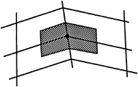
where k=1,6 are the six faces surrounding a particular cell, uk is an average of the velocities from the nodes that define the kth face and Szk are the projected areas in the x direction corresponding to each face. Once the components of the complete stress tensor are computed at the centroids of the cells then the same method of evaluation may be used to compute the viscous fluxes at the vertex through use of equation 7. For this purpose the control volume is now constructed by assembling ![]() fractions of each of the eight cells surrounding a particular vertex. The equivalent two dimensional control volume is sketched in the figure below. This discretization procedure is designed to minimize the error induced by a kink in the grid. It has proved to be accurate and efficient in applications to the solution of three dimensional compressible viscous flows [26,27].
fractions of each of the eight cells surrounding a particular vertex. The equivalent two dimensional control volume is sketched in the figure below. This discretization procedure is designed to minimize the error induced by a kink in the grid. It has proved to be accurate and efficient in applications to the solution of three dimensional compressible viscous flows [26,27].
3.1.3
Time Integration
Equation 8 is integrated in time by an explicit multistage scheme. For each bulk flow time step, the grid, and thus Λijk, is independent of time. Hence equation 8 can be written as
(11)
where the residual is defined as
Rijk(w)=Cijk(w)−Vijk(w)−Dijk(w),
and the cell volume Λijk absorbed into the residual for clarity. If one analyzes a linear model problem corresponding to (11) by substituting a Fourier mode ![]() , the resulting Fourier symbol has an imaginary part proportional to the wave speed, and a negative real part proportional to the diffusion. Thus the time stepping scheme should have a stability region which contains a substantial interval of the negative real axis, as well as an interval along the imaginary axis. To achieve this it pays to treat the convective and dissipative terms in a distinct fashion. Thus the residual is split as
, the resulting Fourier symbol has an imaginary part proportional to the wave speed, and a negative real part proportional to the diffusion. Thus the time stepping scheme should have a stability region which contains a substantial interval of the negative real axis, as well as an interval along the imaginary axis. To achieve this it pays to treat the convective and dissipative terms in a distinct fashion. Thus the residual is split as
Rijk(w)=Cijk(w)+Dijk(w)
where Cijk(w) is the convective part and Dijk(w)=−(Vijk+Dijk) the dissipative part. Denote the time level nΔt by a superscript n, and drop the subscript for clarity. Then the multistage time stepping scheme is formulated as
w(n+1,0)=wn
…
w(n+1,k)=wn−αkΔt(C(k−1)+D(k−1))
…
wn+1=w(n+1,m)
where the superscript k denotes the k-th stage, αm=1, and
C(0)=C(wn), D(0)=D(wn)
The coefficients αk are chosen to maximize the stability interval along the imaginary axis, and the coefficients βk are chosen to increase the stability interval along the negative real axis.
A five-stage scheme with three evaluations of dissipation has been found to be particularly effective. Its coefficients are
α1=1/4 β1=1
α2=1/6 β2=0
α3=3/8 β3=0.56
α4=1/2 β4=0
α5=1 β5=0.44
The actual time step Δt is limited by the Courant number (CFL), which states that the fastest waves in the system may not be allowed to propagate farther than the smallest grid spacing over the course of a time step. In this work, local time stepping is used such that regions of large grid spacing are permitted to have relatively larger time steps than regions of small grid spacing. Of course the system wave speeds vary locally and must be taken into account as well. The final local time step is thus computed as,
where λijk is the sum of the spectral radii of both the convective and viscous flux Jacobian matrices in the x, y and z directions. In regions of small grid spacing and/or regions of high characteristic wave speeds, the time step will be smaller than elsewhere.
3.1.4
Residual Averaging
The allowable Courant number may be increased by smoothing the residuals at each stage using the following product form in three dimensions [18]
where ![]() and
and ![]() are smoothing coefficients and the
are smoothing coefficients and the ![]() are central difference operators in computational coordinates. Each residual Rijk is thus replaced by an average of itself and the neighboring residuals.
are central difference operators in computational coordinates. Each residual Rijk is thus replaced by an average of itself and the neighboring residuals.
3.1.5
Multigrid Scheme
Very rapid convergence to a steady state is achieved with the aid of a multigrid procedure. The idea behind the multigrid strategy is to accelerate evolution of the system of equations on the fine grid by introducing auxiliary calculations on a series of coarser grids. The coarser grid calculations introduce larger scales and larger time steps with the result that low-frequency error components may be efficiently and rapidly damped out. Auxiliary grids are introduced by doubling the grid spacing, and values of the flow variables are transferred to a coarser grid by the rule
where the subscripts denote values of the grid spacing parameter (ie. h is the finest grid, 2h, 4h, …are successively coarser grids) and T2h,h is a transfer operator from a fine grid to a coarse grid. The transfer operator picks flow variable data at alternate points to define coarser grid data as well as the coarser grid itself. A forcing term is then defined as
where R is the residual of the difference scheme. To update the solution on the coarse grid, the multistage scheme is reformulated as
…
…
where R(q) is the residual of the qth stage. In the first stage, the addition of P2h cancels R2h(w(0)) and replaces it by ΣRh(wh), with the result that the evolution on the coarse grid is driven by the residual on the fine grid. The result ![]() now provides the initial data for the next grid
now provides the initial data for the next grid ![]() and so on. Once the last grid has has been reached, the accumulated correction must be passed back through successively finer grids. Assuming a three grid scheme, let
and so on. Once the last grid has has been reached, the accumulated correction must be passed back through successively finer grids. Assuming a three grid scheme, let ![]() represent the final value of w4h. Then the correction for the next finer grid will be
represent the final value of w4h. Then the correction for the next finer grid will be
where Ia, b is an interpolation operator from the coarse grid to the next finer grid. The final result on the fine grid is obtained in the same manner:
The process may be performed on any number of successively coarser grids. The only restriction in the present work being use of a structured grid whereby elements of the coarsest grid do not overlap the ship hull. A 4-level “W-cycle” is used in the present work for each time step on the fine grid [18].
3.1.6
Grid Refinement
The multigrid acceleration procedure is embedded in a grid refinement procedure to further reduce the computer time required to achieve steady state solutions on finely resolved grids. In the grid refinement procedure the flow equations are solved on coarse grids in the early stages of the simulation. The coarse grids permit large time steps, and the flow field and the wave pattern evolve quite rapidly. When the wave pattern approaches a steady state, the grid is refined by doubling the number of grid points in all directions and the flow variables and free surface location are interpolated onto the new grid. Computations then continue using the finer grid with smaller time steps. The multigrid procedure is applied at all stages of the grid refinement to accelerate the calculations on each grid in the sequence, producing a composite “full multigrid” scheme which is extremely efficient.
3.2
Free Surface Solution
Both a kinematic and dynamic boundary condition must be imposed at the free surface. For the fully nonlinear condition, the free surface must move with the flow (ie. up or down corresponding to the wave height and location) and the boundary conditions applied on the distorted free surface. Equation 3 can be cast in a form more amenable to numerical computations by introducing a curvilinear coordinate system that transforms the curved free surface β(x,y) into computational coordinates β(ξ,η). This results in the following transformed kinematic condition
(12)
where ũ and ![]() are contravariant velocity components given by
are contravariant velocity components given by
The free surface kinematic equation may now be expressed as
where Qij(β) consists of the collection of velocity and spacial gradient terms which result from the discretization of equation 12. Note that this is not the result of a volume integration and thus the volume (or actually area) term does not appear in the residual as in the FVM formulation. Throughout the interior of the (x,y) plane, all derivatives are computed using the second order centered difference stencil in computational coordinates ξ and η. On the boundaries a second order centered stencil is used along the boundary tangent and a first order one sided difference stencil is used in the boundary normal direction.
As was necessary in the FVM formulation for the bulk flow, background dissipation must be added to prevent decoupling of the solution. The method used to compute the dissipative terms borrows from a two dimensional FVM formulation and appears as follows:
Dij=Dξ+Dη
where
Dξij=dξi+1,j−dξi,j
and
The expression for α may be written as
where J is the sum of the cell Jacobians and ![]() is used to manually adjust the amount of dissipation. Hence the system of equations for the free surface is expressed as
is used to manually adjust the amount of dissipation. Hence the system of equations for the free surface is expressed as
where
Rij=Qij−Dij.
The same scheme used to integrate equation 11 is also used here. Once the free surface update is accomplished the pressure is adjusted on the free surface such that
The free surface and the bulk flow solutions are coupled by first computing the bulk flow at each time step, and then using the bulk flow velocities to calculate the movement of the free surface. After the free surface is updated, its new values are used as a boundary condition for the pressure on the bulk flow for the next time step. The entire iterative process, in which both the bulk flow and the free surface are updated at each time step, is repeated until some measure of convergence is attained; usually steady state wave profile and wave resistance coefficient.
Since the free surface is a material surface, the flow must be tangent to it in the final steady state. During the iterations, however, the flow is allowed to leak through the surface as the solution evolves towards the steady state. This leakage, in effect, drives the evolution equation. Suppose that at some stage, the vertical velocity component w is positive (cf. equation 3 or 12). Provided that the other terms are small, this will force βn+1 to be greater than βn. When the time step is complete, ψ is adjusted such that ψn+1>ψn. Since the free surface has moved farther away from the original undisturbed upstream elevation and the pressure correspondingly increased, the velocity component w (or better still q · n where ![]() and F=z−β(x,y)) will then be reduced. This results in a smaller Δβ for the next time step. The same is true for negative vertical velocity, in which case there is mass leakage into the system rather than out. Only when steady state has been reached is the mass flux through the surface zero and tangency enforced. In fact, the residual flux leakage could be used in addition to drag components and pressure residuals as a measure of convergence to the steady state.
and F=z−β(x,y)) will then be reduced. This results in a smaller Δβ for the next time step. The same is true for negative vertical velocity, in which case there is mass leakage into the system rather than out. Only when steady state has been reached is the mass flux through the surface zero and tangency enforced. In fact, the residual flux leakage could be used in addition to drag components and pressure residuals as a measure of convergence to the steady state.
This method of updating the free surface works well for the Euler equations since tangency along the hull can be easily enforced. However, for the Navier-Stokes equations the no-slip boundary condition is inconsistent with the free surface boundary condition at the hull/waterline intersection. To circumvent this difficulty the computed elevation for the second row of grid points away from the hull is extrapolated to the hull. Since the minimum spacing normal to the hull is small, the error due to this should be correspondingly small, comparable with other discretization errors. The treatment of this intersection for the Navier-Stokes calculations, should be the subject of future research to find the most accurate possible procedure.
4
Results
4.1
Computational Conditions
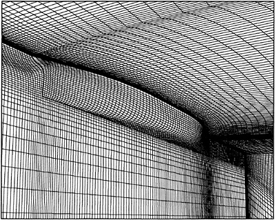
Figures 2 and 3 show portions of the fine grids used for the Navier-Stokes calculations. The number of grid points is 193, 65 and 49 in the x, y and z-directions respectively, and the H—H type grid is used. Grid points are clustered near the bow and stern with a minimum spacing of 0.005 dimensionless units based on the hull length. The grid extends ![]() ship length upstream from the bow,
ship length upstream from the bow, ![]() ship lengths downstream from the stern,
ship lengths downstream from the stern, ![]() ship lengths to starboard, and 1 ship length down below the undisturbed free surface. The minimum spacing in the y-direction, normal to the hull surface, is 0.0001 for the Navier-Stokes computations and 0.0025 for the Euler computations. The resolution on the hull surface is 97 by 17 for the Wigley hull and 97 by 25 for the Series 60. Only the number of grid points in the y-direction is changed for the Euler calculations; rather than 65 the number is 49.
ship lengths to starboard, and 1 ship length down below the undisturbed free surface. The minimum spacing in the y-direction, normal to the hull surface, is 0.0001 for the Navier-Stokes computations and 0.0025 for the Euler computations. The resolution on the hull surface is 97 by 17 for the Wigley hull and 97 by 25 for the Series 60. Only the number of grid points in the y-direction is changed for the Euler calculations; rather than 65 the number is 49.
The following subsections present the computational results for the Wigley hull and the Series 60, Cb=0.6 hull.
4.2
Wigley Hull
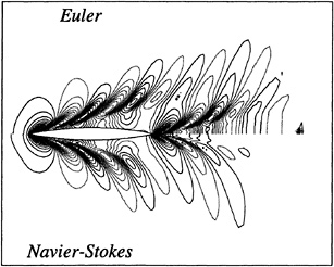
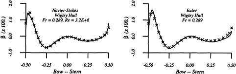
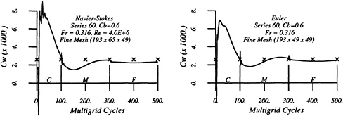
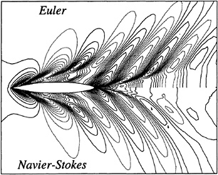
Figures 4 through 9 display computed and experimental results for the Wigley hull at Froude numbers 0.250 and 0.289. Both the Euler and the Navier-Stokes results for the waterline profile along the hull show good agreement with the experimental data [28]. Discrepancies are noted in the stern region where the Navier-Stokes model produces a slight flattening of the wave profile but correctly captures the aft-most waterline elevation, whereas the Euler model shows no tendency to flatten the wave profile but incorrectly predicts the aft-most waterline elevation. The computed wave drag (cf. fig. 5), obtained by integrating the longitudinal component of pressure on the wetted hull surface, shows favorable agreement with the experimentally determined value, Cw(exp)=0.821. The experimental wave drag is inferred by subtracting an estimate of the friction drag from the total drag or by wave analysis. Note that the computed wave drag is evaluated after each multigrid cycle and hence the evolution of the drag is plotted vs. the steady state drag (marked by the x's) determined experimentally. The capital letters C, M and F refer to coarse, medium and fine grids respectively in the grid refinement procedure. The comparisons between computed overhead profiles show agreement between the two methods, except in the stern region and aft where viscous effects cause separation of the flow and a reduction in the amplitudes of the downstream waves (cf. fig. 6).
Essentially the same behavior is noted for the Fr=0.289 case in the next set of figures. The waterline profile is predicted almost exactly for the Navier-Stokes simulation whereas the Euler case predicts a lower waterline level at the stern region. The computed values of the wave drag are in good agreement with the experimentally determined value Cw,exp=1.18.
Figures 11 and 10 are included to show the computed velocity profile at the hull/waterline intersection. The prediction of separation is clearly evident in the stern region of the hull.
4.3
Series 60, Cb=0.6 Hull
In contrast to the Wigley hull, which is an idealized shape, the Series 60 hull is a practical geometry for an actual ship hull. The only major difference in the method of computing the flow about this hull and the Wigley model is the effort required to maintain the proper hull shape as the grid is distorted by the moving free surface. To accomplish this, a grid is produced for the entire hull, both above and below the undisturbed free surface. Spline coefficients are then determined for the entire grid and stored. A new grid is then produced with the uppermost plane of points residing in the plane of the undisturbed waterline at z=0. With the stored spline data the grid is now easily updated as the free surface evolves by redistributing points at intervals of equally spaced arc length. It was found that this method prevents the grid lines from crossing at the close tolerances required for the viscous computations.
The waterline contours shown in figure 12 are in reasonably good agreement for both the Euler and Navier-Stokes simulations. Except for the bow region, it appears that the Euler method does an equally good job, if not better, than the Navier-Stokes method. There is some discrepancy amidship in the Navier-Stokes computation which is possibly due to the method used to update points on the hull/waterline intersection set of points. However, as in the Wigley cases, the drag calculation is in good agreement with experiment (Cw,exp=2.6) [29] and the overhead profiles show good agreement with each other.
5
Conclusions
The objective of the present work was to develop an efficient method to compute Euler and Navier-Stokes solutions for the nonlinear ship wave problem. The results for the Wigley hull and Series 60 hull suggest that the objective has been reached and the resulting computer code has been validated, at least for the range of test cases examined. The wave elevations predicted by the numerical simulations are in excellent agreement with the experimental measurements. In addition, the computed wave drag is in good agreement with the wave drag inferred from the experiments.
The Euler method, which requires significantly less computational resources than the Navier-Stokes method, produces results that appear to be within a reasonable degree of accuracy for engineering design work. As the present method is refined and improved, and applied to other geometries (such as submarines, sailing yachts and more practical stern flows), it is planned to continue the comparison between the two methods in order to establish the conditions under which the Euler method can be expected to give accurate results.
The computational times for the simulations are approximately 10 and 12 hours for the Euler calculations on the Wigley and Series 60 hulls, respectively, and approximately 18 hours for the Navier-Stokes calculations for both hulls. The Euler simulations consist of 100 steps on a 49×13×13 grid, 200 steps on a 97×25×25 grid and 200 steps on a 193×49×49 grid. The Navier-Stokes simulations consist of 100 steps on a 49×17×13 grid, 200 steps on a 97×33×25 grid and 200 steps on a 193×65×49 grid. These times were recorded in calculations using a single processor Convex 3400 computer with 64-bit arithmetic. For the given resolution they appear to represent about a ten-fold decrease in the CPU times reported in the earlier literature, which have usually been presented for coarser grids. The CPU time required for the free surface update and regriding procedures is approximately seven percent that required for the bulk flow calculations.
Acknowledgment
The authors gratefully appreciate the contribution of James Reuther (NASA-Ames) for his time and effort spent helping construct the grids used for the Series 60 hull. We would also like to thank Dr. Takanori Hino for the many helpful discussions concerning this work during his research appointment at Princeton. Our work has benefited greatly from the support of the Office of Naval Research through Grant N00014 –93-I-0079, under the supervision of Dr. E.P.Rood.
References
[1] Toda, Y., Stern, F., and Longo, J., “Mean-Flow Measurements in the Boundary Layer and Wake and Wave Field of a Series 60 CB=0.6 Ship Model-Part1: Froude Numbers 0.16 and 0.316,” Journal of Ship Research, v. 36, n. 4, pp. 360–377, 1992.
[2] Longo, J., Stern, F., and Toda, Y., “Mean-Flow Measurements in the Boundary Layer and Wake and Wave Field of a Series 60 CB=0.6 Ship Model-Part2: Effects on Near-Field Wave Patterns and Comparisons with Inviscid Theory”, Jourmal of Ship Research, v. 37, n. 1, pp. 16–24, 1993.
[3] Hino, T., “Computation of Free Surface Flow Around an Advancing Ship by the Navier-Stokes Equations”, Proceedings, Fifth International Conference on Numerical Ship Hydrodynamics, pp. 103–117, 1989.
[4] Miyata, H., Toru, S., and Baba, N., “Difference Solution of a Viscous Flow with Free-Surface Wave about an Advancing Ship”, Journal of Computational Physics, v. 72, pp. 393–421, 1987.
[5] Miyata, H., Zhu, M., and Wantanabe, O., “Numerical Study on a Viscous Flow with Free-Surface Waves About a Ship in Steady Straight Course by a Finite-Volume Method”, Journal of Ship Research, v. 36, n. 4, pp. 332–345, 1992.
[6] Tahara, Y., Stern, F., and Rosen, B., “An Interactive Approach for Calculating Ship Boundary Layers and Wakes for Nonzero Froude Number”, Journal of Computational Physics, v. 98, pp. 33–53, 1992.
[7] Chen, H.C., Patel, V.C., and Ju, S., “Solution of Reynolds-Averaged Navier-Stokes Equations for Three-Dimensional Incompressible Flows”, Journal of Computational Physics, v. 88, pp. 305–336, 1990.
[8] Rosen, B.S., Laiosa, J.P., Davis, W.H., and Stavetski, D., “SPLASH Free-Surface Flow Code Methodology for Hydrodynamic Design and Analysis of IACC Yachts”, The Eleventh
Chesapeake Sailing Yacht Symposium, Annapolis, MD, 1993.
[9] Chorin, A., “A Numerical Method for Solving Incompressible Viscous Flow Problems ”, Journal of Computational Physics, v. 2, pp. 12–26, 1967.
[10] Rizzi, A., and Eriksson, L., “Computation of Inviscid Incompressible Flow with Rotation”, Journal of Fluid Mechanics, v. 153, pp. 275– 312, 1985.
[11] Dreyer, J., “Finite Volume Solutions to the Unsteady Incompressible Euler Equations on Unstructured Triangular Meshes”, M.S. Thesis, MAE Dept., Princeton University, 1990.
[12] Kodama, Y., “Grid Generation and Flow Computation for Practical Ship Hull Forms and Propellers Using the Geometrical Method and the IAF Scheme”, Proceedings, Fifth International Conference on Numerical Ship Hydrodynamics, pp. 71–85, 1989.
[13] Turkel, E., “Preconditioned Methods for Solving the Incompressible and Low Speed Compressible Equations”, ICASE Report 86–14, 1986.
[14] Jameson, A., Baker, T., and Weatherill, N., “Calculation of Inviscid Transonic Flow Over a Complete Aircraft”, AIAA Paper 86–0103, AIAA 24th Aerospace Sciences Meeting, Reno, NV, January 1986.
[15] Jameson, A., “Computational Aerodynamics for Aircraft Design”, Science, v. 245, pp. 361– 371, 1989.
[16] Jameson, A., “Solution of the Euler Equations for Two Dimensional Transonic Flow by a Multigrid Method”, Applied Math. and Computation, v. 13, pp. 327–356, 1983.
[17] Jameson, A., “Computational Transonics”, Comm. Pure Appl. Math., v. 41, pp. 507–549, 1988.
[18] Jameson, A., “A Vertex Based Multigrid Algorithm For Three Dimensional Compressible Flow Calculations”, ASME Symposium on Numerical Methods for Compressible Flows, Annaheim, December 1986.
[19] Farmer, J., “A Finite Volume Multigrid Solution to the Three Dimensional Nonlinear Ship Wave Problem”, Ph.D. Thesis, MAE 1949-T, Princeton University, January 1993.
[20] Farmer, J., Martinelli, L., and Jameson, A., “A Fast Multigrid Method for Solving Incompressible Hydrodynamic Problems with Free Surfaces”, Accepted for publication in the AIAA Journal, 1993.
[21] Orlanski, I., “A Simple Boundary Condition for Unbounded Hyperbolic Flows”, Journal of Computational Physics, v. 21, 1976.
[22] Baldwin, B.S., and Lomax, H., “Thin Layer Approximation and Algebraic Model for Separated Turbulent Flows”, AIAA Paper 78–257, AIAA 16th Aerospace Sciences Meeting, Reno, NV, January 1978.
[23] Yang, C-I., Hartwich, P-M., and Sundaram, P., “Numerical Simulation of Three-Dimensional Viscous Flow around a Submersible Body”, Proceedings, Fifth International Conference on Numerical Ship Hydrodynamics, pp. 59–69, 1989.
[24] Martinelli, L., “Calculations of Viscous Flows with a Multigrid Method”, Ph.D. Thesis, MAE 1754-T, Princeton University, 1987.
[25] Martinelli, L. and Jameson, A., “Validation of a Multigrid Method for the Reynolds Averaged Equations ”, AIAA Paper 88–0414, AIAA 26st Aerospace Sciences Meeting, Reno, NV, January 1988.
[26] Liu, F. and Jameson, A., “Multigrid Navier-Stokes Calculations For Three-Dimensional Cascades ”, AIAA Paper 92–0190, AIAA 30th Aerospace Sciences Meeting, Reno, NV, January 1990.
[27] Martinelli, L., Jameson, A., and Malfa, E., “Numerical Simulation of Three-Dimensional Vortex Flows Over Delta Wing Configurations”, Lecture Notes in Physics, Volume 414. Thirteenth International Conference on Numerical Methods in Fluid Dynamics, . M.Napolitano and F.Sabetta (Eds.), Rome, Italy, 1992.
[28] “Cooperative Experiments on Wigley Parabolic Models in Japan”, 17th ITTC Resistance Committee Report, 2nd ed., 1983.
[29] Toda, Y., Stern, F., and Longo, J., “Mean-Flow Measurements in the Boundary Layer and Wake and Wave Field of a Series 60 CB=0.6 Ship Model for Froude Numbers .16 and .316”, IIHR Report No. 352, Iowa Institute of Hydraulic Research, The University of Iowa, Iowa City, Iowa, 1991.


DISCUSSION
by Professor J.Feng, Penn State University
-
The definition of Г, the artificial sound speed, given by the authors works well for Euler solvers, but needs further attention in viscous region where the size of time is controlled by restrictions from viscous terms in a N-S solver. Did the authors rescale the Г in the viscous region for their calculations, or probably, for the problem concerned, it is not important (high Reynolds number/thin boundary layer).
-
The coefficients ακ, βκ, (κ=1,2,5) look very interesting. Could the authors explain briefly on the principles and procedures in deriving these coefficients?
Author's Reply
-
In the viscous boundary layer the velocity will tend toward zero due to the no-slip boundary condition s the normal distance to the ship hull tends to zero. When the velocity becomes low in this region Г becomes small as can be seen from the definition in the text. To prevent Г from tending toward zero a cut-off value is introduced such that Г never becomes less than 0.25. Note that the same cut-off value must be used in a stagnation region as well. There is no other special treatment for the artificial compressibility parameter.
-
The coefficients ακ are chosen to maximize the stability limit along the imaginary axis and the βκ are chosen to maximize the stability limit along the negative real axis. The coefficients are typically chosen through analysis of a model one-dimensional convection/diffusion equation. For information regarding the selection of the coefficients which maximize the stability region refer to the following reference; Jameson, A., “Transonic Flow Calculations,” MAE Report #1651, Princeton University, 1984. This reference is also included in Lecture Notes in Mathematics, 1127, edited by F.Brezzi, Springer Verlag, 1985, pp. 156–242.
DISCUSSION
by Dr. David Hally, DREA, Dartmouth
Could you please describe how you generated your grids and what calculations must be done to make them conform dynamically to the free surface?
Author's Reply
The grid for the Wigley hull was constructed analytically using straight lines projecting away from the hull. The grid for the Series 60 was constructed using the GRIDGEN grid generator. Both grids are initially constructed using the entire hull surface, including that portion above the waterline. The grid lines running in the vertical direction are then splined and the coefficients stored. All the grid points above the waterline are then shifted below the waterline with the uppermost plane of points residing on the undisturbed waterline. At this point the flow calculations commence and distortion of the mesh is accomplished by redistributing the grid points, above and below the waterline, according to the current free surface value of β and the stored spline information. It is important to note that the grid is only “generated” once, before the calculations commence. The spline data from the original grid is used to update the grid points by the flow solver as the simulation proceeds.
A Finite-Volume Method with Unstructured Grid for Free Surface Flow Simulations
T.Hino (Ship Research Institute, Japan)
L.Martinelli and A.Jameson (Princeton University, USA)
ABSTRACT
An unstructured grid method developed initially for the transonic inviscid flow is applied to free surface problems around submerged hydrofoils. The flow domain around a submerged body is divided into triangular cells, which makes up the unstructured grid system fitted to a free surface boundary. The incompressible Euler equations and the continuity equation with artificial compressibility are discretized by the finite-volume method in the unstructured grid. Time integration is made by the Runge-Kutta method. Nonlinear free surface conditions are implemented in the scheme. Several techniques for convergence acceleration are used, including the local time steeping, the residual smoothing and the unstructured multigrid. The outline of numerical procedure is presented together with the results of applications. Comparisons of the results with experimental data prove accuracy and efficiency of the present method.
NOMENCLATURE
|
CFL |
Courant number |
|
D |
dissipation term |
|
F |
Froude number |
|
f |
flux in x-direction |
|
g |
gravitational constant |
|
g |
flux in y-direction |
|
h |
wave height |
|
|
interpolation operator in multigrid scheme |
|
L |
chord length of hydrofoil |
|
P |
pre-conditioning matrix |
|
Pk |
forcing function in multigrid scheme |
|
p |
pressure without hydrostatic component |
|
|
pressure |
|
|
residual transfer operator in multigrid scheme |
|
Q |
convective term |
|
R |
residual |
|
s |
submergence of hydrofoil |
|
|
solution transfer operator in multigrid scheme |
|
t |
time |
|
u |
velocity in x-direction |
|
ν |
velocity in y-direction |
|
w |
solution vector |
|
x |
horizontal Cartesian coordinate |
|
y |
vertical Cartesian coordinate |
|
αm |
parameters in Runge-Kutta scheme |
|
β2 |
artificial compressibilty parameter |
|
βqr |
parameter of Runge-Kutta scheme |
|
γ(x) |
damping term of wave height equation |
|
γqr |
parameter of Runge-Kutta scheme |
|
|
parameter of residual smoothing |
|
λ |
wave speed |
INTRODUCTION
Free surface flows have significant importance in ship hydrodynamics. Wave resistance is the major part of the resistance that determines the
propulsive performance of ships. Also, waves generated by a ship interact with the boundary layer along a ship hull and affect stern flows which are important for a propeller design. Motions of ships or floating marine structures in ocean waves are of practical importance. Impact loads due to the large ocean waves sometimes damage ships or marine structures. A number of methods have been developed to solve these free surface problems. However, the nonlinearity of the problems makes it difficult to predict the properties of free surface flows accurately and efficiently.
Rapid development of computer hardwares and softwares in recent years enables the large-scale computation. Thus, Computational Fluid Dynamics (CFD) becomes another way to analyze flow properties. CFD activities in ship hydrodynamics have been mainly for the prediction of viscous flows around a ship stern[1,2] in which free surface is treated as a symmetric boundary. Free surface flows have been treated by a kind of a panel method assuming inviscid flows[3]. However, because there are interactions between viscous flows and free surface waves, it is desirable to solve viscous flow problems under free surface effects. Attempts to this direction are Hino[ 4], Miyata et al.[5], Tahara et al.[6] and so on.
When one solves nonlinear free surface flows around a ship with a boundary-fitted grid, which is common in the recent CFD method, a grid must be generated at each time step, because free surface is dynamic in time. The grid generation is not an easy task even without a free surface movement when the body geometry becomes complex. Free surface deformations which are large particularly near the body gives additional complexity to the grid generation.
CFD in aerodynamics is much older than its counterpart in ship hydrodynamics. Various new technologies have been invented in the CFD for aerodynamics. Among them, Jameson et al.[7] developed unstructured grid method for transonic flow computations which uses the triangular grid rather than rectilinear grid in the structured grid case. Later, this method is applied to incompressible flow problems by introducing the artificial compressibility[8]. This unstructured grid method has capability to cope with the geometrical complexity and therefore suitable for free surface flow problems.
In this paper, an unstructured grid method is applied to free surface problems. The problems concerned are flows around a submerged hydrofoils. This is chosen partly because the problem is much simpler compared with flows around a surface-piercing body and partly because the original method is for transonic aerofoils and can be naturally extended to hydrofoil problems.
The governing equations are incompressible Euler equations. Though the final goal of the study is the viscous flow computations, the Euler equations are selected as the governing equation for its simplicity. Artificial compressibility is introduced in the continuity equation. This makes the system of equations hyperbolic and the well-developed efficient techniques to solve hyperbolic equations can be used.
NUMERICAL PROCEDURES
Governing Equations
Governing equations are two-dimensional incompressible Euler equations and are expressed in the form non-dimensionalized by the chord length of a hydrofoil L, the uniform flow velocity U and the fluid density ρ as follows:
(1)
(2)
(3)
where (x,y) are Cartesian coordinates (y is upward positive) and (u,ν) are the velocity components in (x,y) directions, respectively. ![]() is the static pressure and t is time. F is Froude number defined using the gravitational constant g as
is the static pressure and t is time. F is Froude number defined using the gravitational constant g as
(4)
Since there is no term associated with the time derivative of pressure in the governing equations (1)–(3), difficulties come out when one solves these equations in the time-marching manner. Usually pressure field is computed by the Poisson equation which is derived from the divergence of the momentum equations (2)–(3) and the continuity equation (1) in such a way that the velocity field satisfies the continuity condition at each time step [9].
When only the steady state solution is required, the alternative approach called the artificial compressibility method can be used. In this
method first proposed by Chorin [10], the continuity equation is modified by introducing the pseudo-compressibility as follows:
(5)
where β2 is the artificial compressibility parameter. When the solution becomes steady, the equation (5) recovers the original form (3). Since the system of equations (5), (2) and (3) is hyperbolic, efficient numerical solution methods for the hyperbolic equations can be applied.
The parameter β2 is determined by using the local velocity magnitude as
(6)
where rb is a global constant and the parameter ![]() is used to prevent β2 from approaching zero near the stagnation point. rb=5 and
is used to prevent β2 from approaching zero near the stagnation point. rb=5 and ![]() =0.3 are typical values in the present study.
=0.3 are typical values in the present study.
Eqs.(5), (2) and (3) can be rewritten in the vector form as
(7)
where
(8)
and p is the pressure without the hydrostatic component, i.e.,
(9)
P is a matrix defined as
(10)
Boundary conditions needed for free surface flow problems are a body surface condition, a free surface condition and a far field condition. The first one is the free-slip condition in case of the inviscid flow, that is,
u nx+ν ny=0 (11)
where (nx, ny) are the unit vector outward normal to the body surface.
The second one, the free surface condition consists of two conditions. One is the dynamic condition that states the continuity of stresses on the air-liquid interface. For the inviscid case this is expressed as
(12)
or, equivalently,
![]() y=h (13)
y=h (13)
where p0 is atmospheric pressure (assumed to be constant) and y=h(x;t) is the free surface location. The other free surface condition is called the kinematic condition that means the fluid particles on the free surface keep remaining on it. This is written as
(14)
The free surface shape can be updated by Eq.(14) in the time-marching manner.
The far field conditions are as follows. At far upstream, flow is uniform and free surface is undisturbed. On the other hand, the waves generated by a hydrofoil propagate to far down stream. Water depth is assumed infinite.
Spatial Discretization
Finite-Volume Method
In a finite-volume formulation a solution domain is divided into small cells. The present method employs unstructured grid in which every cell is triangular. One of the superiorities of unstructured grids over structured ones is its flexibility to deal with complex geometry. Therefore, unstructured grids are particularly suitable to free surface flow problems in which the deformation of free surface boundary causes further geometrical complexity in addition to that of body configuration.
The flow variables (u,ν) and p are defined at the vertices of each triangle. The control volume for a given node i is taken as the union of all the triangles which share that node as a vertex as shown in Fig.1. The integration of the governing equation (7) over this control volume yields
(15)
where Ω means the control volume and ∂Ω is its boundary. Since the grid is aligned to the free

Figure 1: Control volume around the node i
surface boundary which moves in time, the grid is time-dependent and the effects of grid movement must be taken into account for the time-accurate computation. However, since the present method employs the steady state formulation and the transient solution does not have physical meaning, one can make approximation to drop all the terms associated with the grid movement. Thus, f and g in Eq.(15) have the same form as in Eq.(8). In the discrete form, Eq.(15) becomes
(16)
where Si is the area of the control volume around the node i which is computed by the summation of the area of each triangle in the control volume. The summation in Eq.(16) is taken over all the edges surrounding the control volume and ne is the number of the edges. Also, (Δyk,−Δxk) gives the unscaled outward normal vector of the k-th edge. fk and gk are the flux vectors evaluated by taking average of the values at both ends of the edge. This discretization corresponds to the central difference scheme in the structured grid case. The time integration scheme for Eq.(16) is described in the subsequent section.
Artificial Dissipation
Since the evaluation of Eq.(16) described above is the scheme equivalent to the central difference scheme for the Euler equations, this scheme is not stable due to the decoupling of neighboring node unless one adds the artificial dissipation terms to the equations. To keep the second order accuracy of the scheme, the fourth-order dissipation models are used in the scheme, while the second-order dissipation terms used in the compressible flow code [11] to prevent oscillation near shocks are not used.
By adding the artificial dissipation terms, Eq.(16) is rewritten as
(17)
where
(18)
and Di(w) is the dissipation terms. The dissipation terms are evaluated as follows. First, the undivided Laplacian in the computational space is approximated as,
(19)
The dissipation terms are constructed by using this ![]() as
as
(20)
where ![]() is a global constant which controls the amount of dissipation and λij is a scale factor. The summation is taken over all the nodes on the boundary of the control volume around the node i and nn is the number of the nodes.
is a global constant which controls the amount of dissipation and λij is a scale factor. The summation is taken over all the nodes on the boundary of the control volume around the node i and nn is the number of the nodes.
From the analogy to upwind differencing, the scale factor λij is determined as follows. First, the maximum wave speed is determined by the spectral radii of the flux Jacobian matrices as
λ=ρ(AΔy−BΔx) (21)
where
 , (22)
This yields
(23)
Thus, a scale factor λij which is λ associated with the edge consists of the nodes i and j is defined as
(24)
where
qi=uiΔyij−νiΔxij (25)
(26)
and (Δxij, Δyij) is the vector from the node i to the node j. qj and cj can be evaluated by replacing ui, νi and ![]() in the above equations by uj,νj and
in the above equations by uj,νj and ![]() , respectively.
, respectively.
Boundary Conditions
Body Boundary Condition
Free-slip condition on the body (11) is implemented in the following way. To determine two velocity components (u,ν) on the boundary, two conditions are required. One condition is apparently the free slip condition (11). The other condition is that the tangential velocity does not have gradient in the normal direction, that is,
(27)
where n is the normal direction and qt is the tangential velocity defined by using the unit outward vector on the body (nx, ny) as
qt=u ny−ν nx (28)
For the node which lies on the body boundary, the tangential velocity is extrapolated from the inside in such a way that Eq. (27) is satisfied. First, for each node on the body boundary, the edge from which velocity is extrapolated is searched. Searching procedure is 1) search the triangle that consists of the boundary node under consideration and two internal nodes, 2) the edge formed by the two internal nodes is registered as a candidate edge, 3) from the candidates select the edge in such a way that the angle between the vector from the boundary node to the mid-point of the edge and the outward normal vector of the boundary node is minimum. Thus, the velocity can be extrapolated from the direction approximately normal to the body surface. Suppose that the boundary node is denoted as O and that the end points of the corresponding edge are A and B as shown in Fig. 2, the extrapolation formula is
(qt)o=(1−κ)(qt)A+κ(qt)B (29)

Figure 2: Velocity extrapolation of the boundary node

Figure 3: Control volume for the boundary node
where
(30)
where P is the intersection point between ![]() and the vector normal to the boundary (see Fig. 2). From Eqs.(29) and (11), the velocity component on the body is computed as
and the vector normal to the boundary (see Fig. 2). From Eqs.(29) and (11), the velocity component on the body is computed as
u=(qt)ony, ν=−(qt)onx (31)
The pressure on the body is computed by the modified continuity equation (5). The control volume is taken as shown in Fig. 3. Mass fluxes across the boundary edges are set zero because of the free-slip condition. The discretization is carried out in the usual way except that the node is on the perimeter of the control volume.
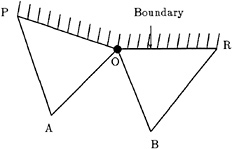
Figure 4: Velocity extrapolation on the free surface
Free Surface Condition
Since the the grid is aligned to the free surface boundary, the free surface dynamic condition (13) is satisfied by simply setting pressure value on the free surface to p0+h/F2.
The velocity on the free surface is extrapolated from inside in such a way that the velocity gradient in the normal direction is zero. Though this can be approximated in the same way as for the body boundary, the simpler extrapolation scheme is preferable because re-calculation of extrapolation coefficient κ at each time-step due to the grid movement is time-consuming. (Note that the grid points close to the body boundary do not move in time as described in the subsequent section.) Suppose that the free surface node O is the common node for the boundary edge ![]() and
and ![]() and these edges are the part of the triangles ΔPOA and ΔOBR, respectively as depicted in Fig.4 (Note that node O, A and B do not necessarily form a triangle), then velocity at node O is computed by
and these edges are the part of the triangles ΔPOA and ΔOBR, respectively as depicted in Fig.4 (Note that node O, A and B do not necessarily form a triangle), then velocity at node O is computed by
(32)
In the above approximation, the mid-point of ![]() is assumed to be in the normal direction from the node O.
is assumed to be in the normal direction from the node O.
The kinematic condition (14) is used to update the free surface shape. The spatial discretization is based on the third-order upwind finite-differencing scheme and the equation for the node i becomes
(33)
where the node numbering is sequential from upstream to downstream and (ui,νi) is the velocity at the node i whose coordinate is given by (xi,hi).
Far Field Conditions
At inflow, flow is uniform, that is,
u=1,ν=0,p=0,h=0 (34)
are given.
At outflow, since waves generated by a hydrofoil propagate to infinite downstream, flow is not uniform. To prevent the reflection of waves to the solution domain, the outflow conditions must be carefully implemented. The open boundary conditions for free surface problems are treated by the various methods [12]. Among them, the procedure used here is the artificial damping method, in which waves going through the outflow boundary is dissipated by adding artificial damping terms in the flow equation.
The free surface kinematic condition is modified as
(35)
where γ is the artificial damping terms defined as
(36)
where A is a constant that controls the amount of damping and xo is the x-coodinate of the outflow boundary. xd is defined as
xd=xo−2πF2 (37)
That is, the damping zone is set one wavelength computed by the linear theory from the outflow boundary. The quadratic form of the damping term in Eq.(36) gives the gradual increase of dissipation, which prevents the reflection of waves at the edge of the damping zone.
Velocity and pressure on the outflow boundary is computed by the control volume of Fig.3, which is equivalentto rhe one-sided differencing.
At the bottom boundary, pressure p is assumed to zero, which corresponds to the hydrostatic value and velocity is computed from the momentum equations with the one-sided differencing using the control volume of Fig.3.
Time Stepping
As the time integration scheme, the explicit multi-stage Runge-Kutta scheme originally developed for compressible flows [11] is used here.
As stated earlier, the grid is time-dependent in the present case, therefore, the control volume is also time-dependent. However, when only steady state solutions are of interest, one can simplify the solution procedure by dropping the terms associated with the grid movement. Suppose that one has the grid and the solution at time step (n), the procedure to proceed one time step is as follows. The flow equations (17) are solved assuming that the grid does not move in time, that is, Si, Δx and Δy appeared in Eq.(17) are evaluated using the grid at time step (n) and are kept constant in time. Thus, Eq.(17) can be rewritten as
(38)
This equation gives an approximated solution at time step (n+1). Then, the free surface kinematic condition (14) is solved in the same manner as the flow equations and the wave height at time step (n+1) is obtained. Next, the grid points are redistributed in such a way that the grid is conformed to the newly computed free surface configuration. During this redistribution process, the number of grid points and the edge connectivity are not changed so as to avoid the re-triangulation at each time step. The flow variables at time step (n+1) are set equal to the values computed under the approximation that the grid is fixed. The geometric quantities Si, Δx and Δy are recomputed by using the new coordinates and the computation proceeds to the next time-step.
Since the grid points do not move in time when a solution becomes steady, this approximated procedure must give the same steady state solutions as the time-accurate scheme does.
Time integration scheme for the flow equation (38) and the wave height equation (14) is the Runge-Kutta method which is a class of one-step multi-stage explicit schemes. The general m-stage solution procedure for Eq.(38) from the time step (p) to (p+1) can be written as follows:
w(0)=wp (39)
(40)
(41)
…
(42)
wp+1=w(m) (43)
where R(q)(w) is the residual evaluated at q-th stage and is defined by the weighted average of the residuals computed by the flow variables of previous stages, i.e.,
(44)
αm, βqr and γqr define the particular scheme. The values of these coefficients for the 4-stage scheme used in this study are as follows.
α1=1/3,α2=4/15,α3=5/9,α4=1 (45)
(46)
γ00=1
γ10=0.5, γ11=0.5
γ20=0.5, γ21=0.5, γ22=0
γ30=0.5, γ31=0.5, γ32=0, γ33=0
(47)
Thus, the dissipation terms are evaluated twice in one time-step.
The free surface kinematic condition (14) is solved in the same manner except that there are no dissipation terms due to the use of upwind differencing.
Grid Generation and Grid Movement
The generation of unstructured triangular grid around a body can be achieved by various ways. Among them, the Delaunay triangulation method [14] and the advancing front method [13] are commonly used in the CFD field. The former is the procedure to establish unique triangulation of given grid points covering solution domain, while the latter is the method to generate points and connect them simultaneously.
The unstructured grid around the submerged hydrofoil used here is generated by the Delaunay triangulation. The set of points are generated by the combination of the conformal mapping around the region close to a foil and the algebraic method in the other region. The conformal mapping is an established way to generate O-grid around a foil of an arbitrary shape. The algebraic method is required since the outer
boundary is rectangular and since the grid spacing control is needed for the better resolution of the free suface region. The points are clustered in the region above and behind the body and near the free surface where the free surface deformation is expected to be large.
The grid movement is carried out in the following way. The initial grid is generated by assuming the flat free surface. On this stage y-coordinate of the uppermost point generated by the conformal mapping is searched and stored as yu. yu is the uppermost extent of the 'inner grid' that is generated in the region close to the body and only the grid point above yu are allowed to move following free surface movement. Assume that the wave height at time step n is given by hn(x), then the grid movement of the node i is defined as
(48)

(49)
where h(xi) is the wave height at x=xi and is computed by the linear interpolation because xi does not necessarily coincide with the x-coordinate of the free surface nodes. Thus, all the points above yu move vertically due to the free surface movement. The moving distance is linearly distributed between hn+1 and yu. By this procedure the grid points near the body do not move and the complicated re-distribution procedure for points near the body is avoided.
Convergence Acceleration Techniques
Three techniques are used to accelerate the convergence of solutions to the steady state in the present scheme. A local time stepping is the method in which the solution at each point proceeds in time with the time step defined locally from the local stability limit, while a residual smoothing is used to increase the bound of the stability limit of the time stepping scheme itself. A multigrid method is an efficient way to accelerate the convergence, where the time stepping is carried out by using successively coarser grids as well as the original finest grid.
Local Time Step
For explicit schemes the maximum permissible time step is limited by the Courant-Friedrichs-Lewy (CFL) condition. In one dimensional case, this is written as
(50)
where CFL is the maximum Courant number permitted by the scheme, Δx is the grid size, and c is the maximum wave speed. When one uses the globally constant time step, Δt must be smaller than the minimum value of CFLΔx/c.
In practice, the grid spacing is not uniform due to the clustering of points. Therefore the time step is determined based on the minimum grid spacing. This yields the small time step and causes slow convergence.
If only steady state solutions are of interest, one can use the locally varying time step at the expense of time-accuracy. The local time step Δti is taken as its maximum permissible value, i.e.,
(51)
In case of unstructured grid employed here, the above equation is modified as
(52)
where Si is the area of the control volume around the node i.
Residual Smoothing
As stated earlier, explicit schemes have the CFL limit of stability. Residual smoothing procedure described below is the way to increase the stability bound of a time stepping scheme. Thus, larger time step can be taken and the fast convergence is achieved. In the method, the residual at the node i, Ri(w) is replaced by implicitly averaged value Ri(w), where
(53)
where ![]() is a constant and the operator
is a constant and the operator ![]() is the undivided Laplacian in the computational space defined in Eq.(19). The resulting linear equation
is the undivided Laplacian in the computational space defined in Eq.(19). The resulting linear equation
(54)
is solved iteratively by the Jacobi method. This gives the implicit property to the scheme and the CFL limit can be larger than the unsmoothed case. One dimensional analysis shows that one can take arbitrary large time step as far as ![]() is taken correspondingly large [11]. In this study
is taken correspondingly large [11]. In this study ![]() is taken 0.5.
is taken 0.5.
Unstructured Multigrid
Multigrid method is known as the efficient way to get fast convergence. The concept of the multigrid time stepping applied to the solution of hyperbolic equations by Jameson [11] is to compute corrections to the solution on a fine grid by the time-stepping on a coarser grid.
The general procedure of the multigrid method is as follows. Equations to be solved is written as
(55)
and the subscript k refers as the grid index.
First, the solution wk is obtained in the fine grid (k) by solving
(56)
by the Runge-Kutta scheme described above. Then, the solution is transferred from the fine grid (k) to the next coarser grid (k+1) by
(57)
where ![]() is a transfer operator. The solution in the coarse grid is updated by solving the equation
is a transfer operator. The solution in the coarse grid is updated by solving the equation
(58)
with the Runge-Kutta scheme and ![]() is obtained. Pk+1 in the above equation is the forcing function in the coarse grid (k+1) defined as
is obtained. Pk+1 in the above equation is the forcing function in the coarse grid (k+1) defined as
(59)
where ![]() is another transfer operator. The first term of the right-hand-side of Eq.([?]) is the residual transferred from the finer grid and the second term is the residual evaluated by the transferred solution. This second term cancels the residuals in the coarse grid only and the driving force comes from only the residual transfered from the finer grid.
is another transfer operator. The first term of the right-hand-side of Eq.([?]) is the residual transferred from the finer grid and the second term is the residual evaluated by the transferred solution. This second term cancels the residuals in the coarse grid only and the driving force comes from only the residual transfered from the finer grid.
![]() gives the correction of the solution at the grid (k+1). This procedure is repeated on successively coarser grid. Finally, after the computation of the correction at the coarsest gird, the correction is transferred back from the coarse grid (k+1) to the fine grid (k) by
gives the correction of the solution at the grid (k+1). This procedure is repeated on successively coarser grid. Finally, after the computation of the correction at the coarsest gird, the correction is transferred back from the coarse grid (k+1) to the fine grid (k) by
(60)
where ![]() is an interpolation operator. The multigrid cycle employed here is V-cycle in which the equations are solved only when the solution moves from the fine grid to the coarse one and the interpolation is used in the transfer of correction from the coarse grid to the fine one.
is an interpolation operator. The multigrid cycle employed here is V-cycle in which the equations are solved only when the solution moves from the fine grid to the coarse one and the interpolation is used in the transfer of correction from the coarse grid to the fine one.

Figure 5: Transfer of solution
In case of the structured grids, the generation of successively coarser grids can be done simply by deleting the alternate points along each grid line. This also makes it easy to define the operators described above. In the unstructured grids, however, neither the grid generation nor the definition of the operators is straightforward.
In the present study, the multigrid strategy of Mavriplis [14] is employed. That is, to keep flexibility of unstructured grids as much as possible, the series of coarser grids are generated independently. The grid generation procedure is repeated fo each grid with changing the grid density parameters.
The operators for the transfers are defined as follows. ![]() is the operator with which the solution w transfers from the fine grid to the coarse one. This is defined as
is the operator with which the solution w transfers from the fine grid to the coarse one. This is defined as
(61)
where I is the node in the coarse grid under concideraton and 1,2 and 3 are the nodes forming the triangle in the fine grid which contain the node I. A1 is the area of the triangle consists of I, 2 and 3 as shown in Fig.5. A2 and A3 are defined similarly.
![]() is the transfer operator of the residuals. The residual at the node I in the coarse grid
is the transfer operator of the residuals. The residual at the node I in the coarse grid

Figure 6: Transfer of residuals
is computed by
(62)
The first summation is over the triangles of coarse grid that share the node I as a common vertex. The second summation is taken over all the nodes in the fine grid that lie inside the triangles determined in the first summation. BI is the area of the triangle consists of the nodes p, II and III as shown in Fig.6. BII and BIII are defined similarly. Thus, the residuals in the coarse grid are linearly distributed to the nodes in the fine grid. Note that this procedure is conservative, that means the grand sum of the residuals in the coarse grid is equal to the grand sum of the residuals in the fine grid. This feature is important, because the the driving force in the coarse grid comes only from the fine grid residuals due to the forcing function (59).
Finally, ![]() is for the interpolation of the corrections in the coarse grid to the fine grid. From Eq.(60) the correction dw is defined by
is for the interpolation of the corrections in the coarse grid to the fine grid. From Eq.(60) the correction dw is defined by
dw=w+−w(0) (63)
The transfer of the correction from the coarse grid to the fine grid is done as follows.
(64)
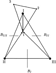
Figure 7: Transfer of correction
where the node 1 is the node of the fine grid and it lies inside the triangle of the nodes I, II and III in the coarse grid as shown in Fig.7. BI is the area of the triangle of 1, II and III. BII and BIII are defined similarly
Since the grid is dynamic in time for the present case, the above operators must be recomputed at each time step using new coordinates of the grid. The most time-consuming part of this re-computation is the search of the triangle in which the certain point lies. The procedure taken here is based on the tree-search algorithm similar to the one used by Mavriplis[14]. First, every triangle has a list of three neighbour triangles. This list does not change by the grid movement because the point connectivity is fixed. At the beginning, the search of the triangle is carried out by the simple search consists of the loop over all the triangles.
The search of triangles after the grid movement are achieved by the following procedure. The search starts with the triangle in which the point under consideration lies before the grid movement. If the point still lies in this triangle, the search ends. If not, the three triangles which are the neighbours of the first triangle are searched next. The search region is extended successively to the neigbours of the neigbours until the desired triangle is found. Since the moving distance of grid points are not large, this search converges usually in a few extensions. The computational time required is much less than that
of the loop over all the triangles.
RESULTS
The numerical procedure described above is applied to free surface flow simulations around a submerged hydrofoil. A hydrofoil section used here is NACA0012 and the angle of attack is set 5 degrees. The depth of submergence 5 measured at the mid-chord and nondimensionalized by the chord length varies from 1.034 to 0.911. Froude number F=0.5672 and water depth is assumed to be infinite. These conditions correspond with the experiments by Duncan [15] except that the experiments were carried out in the tank of a finite water depth (varies from 1.90 to 1.77, nondimensionalized by a chord length).
For all the computation, the initial computational domain is taken as
−7≤x≤6.25, −7≤y≤0 (65)
unless otherwise noted, x=0 is the 1/4 chord aft from the leading edge of the hydrofoil and y=0 is the undisturbed water level.
Three levels of multigrids used for the computation with the submergence s=1.034 are shown in Fig.8. The finest grid consists of 6,587 nodes and 12,854 triangles. Among them, 64 nodes are distributed on the body. The medium grid has 1,642 nodes and 3,130 triangles while the coarsest one has 409 nodes and 745 triangles. Since these grids are for the converged solution, the free surface configurations correspond to the developed wave field, though the initial grids are generated under the undisturbed free surface. Maginified view of the finest grid is depicted in Fig. 9.
The computed pressure distributions with the multi- and single- grid cases are shown in Figs. 10 and 11. Both are the results at 400 time cycles with the Courant number CFL being 5.0.
The single grid case shows the undeveloped wave field in which the waves generated by the hydofoil do not yet reach the outflow boundary, while in the multigrid case the converged solution with developed wave field (except for the region close to the outflow boundary where numerical damping is added) is obtained. This is due to the fact that time advancement in one multigrid cycle in the three-level mutigrid is approximately Δt+2Δt+4Δt=7Δt, where Δt is the time step in the finest grid, because the local time stepping is taken proportional to the cell area. On the other hand, time advancement in the single-grid case in one cycle is just Δt.
For the practical computations shown hereafter the full multigrid scheme is employed, in which the initial solution is obtained with only the coarsest grid, then the solution is transferred to the next finer grid and the solution is updated by the multigrid method using the coarsest grid and the next finer grid. The procedure is repeated with adding one level of multigrid at a time until the finest grid is reached. The cycles for each stage are 1,000 cycles with the single coarsest grid, 500 cycles with the double grid (the medium and the coarsest) and 400 cycles with triple grid (the finest, the medium and the coarsest grids). With this scheme, the residual in the final stage is O(10−4).
The effect of numerical damping expressed by Eq.(36) is verified next. Fig. 12 compares two computed wave configurations. One has the solution domain of −7≤x≤6.25, and the other has the longer domain of −7≤x≤8.25. The number of grid points in the longer domain case increases in such a way that the grid density is approximately the same in both cases. Since Froude number is 0.5672, the length of the damping zone defined in Eq.(37) is about 2.02. Waves going through the outflow boundary are damped effectively in the damping zone and the reflection of waves on the outflow boundary cannot be observed. Also, the comparison of the long-domain solution and the short-domain one shows that the artificial damping does not affect the flow field upstream of the damping zone.
In Fig.13 the computed wave height is compared with the experimental data by Duncan [15]. The present result is in good agreement with the experimental data. Fig.14 and 15 show the pressure distribution and the velocity vectors in the vicinity of the hydrofoil, respectively. Fig.16 shows the computed Cp distribution on the body.
Fig.17 is the result with s=0.951. Again, the computed wave profile shows good agreement with experimental data [15]. When the submergence of the hydrofoil decreases, the wave amplitude becomes larger and wave length becomes shorter than the deep submergence case. These nonlinear features of wave formations in the experiment are clearly captured by the present method. Note that in the experiment with s= 0.951, two types of wave profiles, one is breaking and the other is non-breaking, are obtained depending on the experimental condition. However, the present computation predicts only the non-breaking waves.
When the submergence decreases further
to s=0.911, only the breaking waves exist in the experiment. However, the present method predicts the very steep but non-breaking wave as shown in Fig. 18. In the implementation of the kinematic free surface condition, the wave height is assumed to be expressed by the single-valued function of x. Thus, breaking waves or overturning waves cannot be simulated by the present scheme. However, more flexible treatment of the free surface movement such as the Lagrangian method can be adopted without difficulties. The nature of unstructured grid methods enables the spatial discretization in such a highly deformed region. This improvement together with development of the time-accurate scheme makes it possible to simulate transient breaking or overturning waves in the near future.
CONCLUSIONS
In the present study, a finite-volume method with an unstructured grid method which has been originally developed for transonic flow computations is successfully applied to incompressible flows with a free surface. The computed results for a submerged hydrofoil show good agreement with the experimental data.
Further extensions of this method are the inclusion of viscous effects, transient flow computation using time-accurate scheme, breaking or overturning waves simulation and so on. Also, the three-dimensional version of the present method, already exists for transonic flow computations[16], must be a useful tool for ship hydrodynamics or marine engineering.
ACKNOWLEDGEMENT
This work was done while the first author stayed at Princeton University as a visiting research fellow. He is grateful to Ship Research Institute, Japan and to the Science and Technology Agency of Japanese Government for the support during his stay at Princeton.
REFERENCES
[1] Kodama, Y.: “Grid Generation and Flow Computation for Practical Ship Hull Forms and Propellers Using the Geometrical Method and the IAF Scheme.” , Proc. 5th Intern. Conf. Numerical Ship Hydrodynamics , Hiroshima, ( 1989).
[2] Chen, H.C.: “Solution of Reynolds-Averaged Navier-Stokes Equations for Three-Dimensional Incompressible Flows.”, J. Comput. Phys., Vol.88, ( 1990).
[3] Dawson, C.W.: “A Practical Computer Method for Solving Ship Wave Problems.”, Proc. 2nd Intern. Conf. Numerical Ship Hydrodynamics, Berkeley, ( 1977).
[4] Hino, T.: “Computation of a Free Surface Flow around an Advancing Ship by the Navier-Stokes Equations.”, Proc. 5th Intern. Conf. Numerical Ship Hydrodynamics, Hiroshima, ( 1989).
[5] Miyata, H. et al.: “Difference Solution of a Viscous Flow with Free-Surface Wave about an Advancing Ship.”, J. Comput. Phys., Vol.72, ( 1987).
[6] Tahara, Y. et al.: “An Interactive Approach for Calculating Ship Boundary Layers and Wakes for Nonzero Froude Number.”, J. Comput. Phys., Vol.98, ( 1992).
[7] Jameson, A. et al.: “Finite Volume Solution of the Two-Dimensional Euler Equations on a Regular Triangular Mesh.”, AIAA J., Vol.24, No.4, ( 1986).
[8] Dreyer, J.D.: “Finite Volume Solutions to the Steady Incompressible Euler Equations on Unstructured Triangular Meshes.”, MSE Thesis, Dept. Mechanical and Aerospace Engineering, Princeton University, ( 1990).
[9] Harlow F.H. et al.: “Numerical Calculation of Time-Dependent Viscous Flow of Fluid with Free Surface.”, Physics of Fluids, Vol.8, ( 1965).
[10] Chorin, A, J.: “A Numerical Method for Solving Incompressible Viscous Flow Problems. ”, J. Comput. Phys., Vol.2, ( 1967).
[11] Jameson, A: “Computaional Transonics”, Comm. Pure Appl. Math., Vol.XLI, ( 1988).
[12] Romante, J.E.: “Absorbing Boundary Conditions for Free Surface Waves.”, J. Comput. Phys., Vol.99, ( 1992).
[13] Peraire, J. et al.: “Adaptive Remeshing for Compressible Flow Computations.”, J. Comput. Phys., Vol.72, ( 1987).
[14] Mavriplis, D.: “Solution of the Two-Dimensional Euler Equations on Unstructured Triangular Meshes”, PhD Thesis, Dept. Mechanical and Aerospace Engineering, Princeton University, ( 1987).
[15] Duncan, J.H.: “The Breaking and Non-Breaking Wave Resistance of a Two-Dimensional Hydrofoil.”, J. Fluid Mech., Vol.126, ( 1983).
[16] Jameson, A. et al.: “Calculation of Inviscid Transonic Flow over a Complete Aircraft.”, AIAA paper 86–0103, ( 1986).
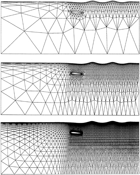


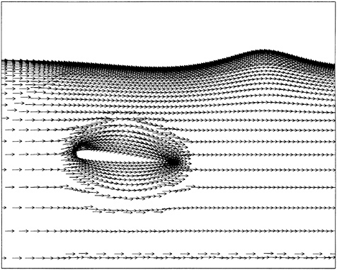
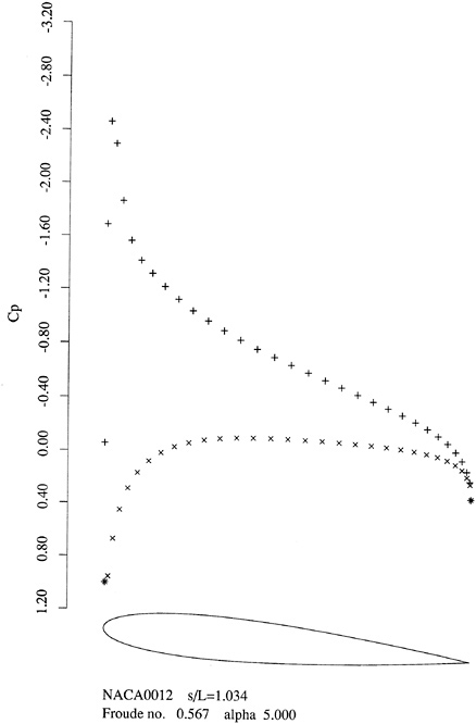


DISCUSSION
by Dr. Antony J.Musker, DRA Haslar, England.
A very sophisticated algorithm has been presented for solving the 2D Euler equations for the free-surface wave-making problem. There is little doubt that an Euler approach will perform better in the near wave-breaking region compared with Rankine source density methods since these fail completely for extreme nonlinear cases. It is not clear, though, how the methodology described in your paper can be expanded to deal with actual wave-breaking. Does your suggestion of adopting a Lagrancian approach imply that one has to start again from first principles or that some modification can be made to the existing approach?
The grid is composed of triangles constructed according to Delaunay criterion. I believe it is a property of this technique that the resulting triangles tend to be not far from equilateral. Although this may work for Euler solvers, it is doubtful that it will work for Navier-Stokes solvers because of the need to resolve the very high velocity gradients close to solid boundaries. Perhaps the authors could comment on this?
Author's Reply
In order to simulate breaking waves, the free surface conditions, both kinematic and dynamic conditions, should be satisfied as accurately as possible. The unstructured grid method shown here can cope with the dynamic condition in case of the complex geometry which may occur in the wave breaking process.
The implementation of the kinematic free surface condition is crucial for breaking wave simulations. The Lagrangean approach may be the most promising way to deal with large deformation such as overturning waves. In the present flow solver, any algorithm for free surface tracking can be used with the proper triangulation procedure of flow domain. The modifications are needed only in the free surface tracking and re-girding routines.
The unstructured grids for the Navier-Stokes solutions require high-aspect-ratio triangles near the solid boundary. The simple Delaunay triangulation does not work well in such cases. However, by using the local mapping, the stretching grid for the viscous computations can be generated by the Delaunay algorithm, see the following reference.
Mavriplis, D.J., “Adaptive Mesh Generation for Viscous Flows Using Delaunay Triangulation, ” Journal of Computational Physics, Vol. 90, No. 2, 1990.
A Semi-Implicit Semi-Lagrangian Finite Element Model for Nonlinear Free Surface Flow
A.Allievi and S.Calisal
(University of British Columbia, Canada)
ABSTRACT
Potential flow initial-boundary value problems describing fluid structure interaction with fully nonlinear free surface boundary conditions have been studied using a mixed Lagrangian Eulerian formulation. The two dimensional boundary value problem has been solved in the physical domain by means of a Bubnov-Galerkin formulation of the Laplace equation. The initial-value problem related to the behavior of some of the moving boundaries has been discretized using a semi-implicit semi-Lagrangian two time level iterative scheme that is almost free from smoothing.
Fluid responses to periodic excitation of surface piercing and submerged bodies have been calculated. The impulsive response of tanks of various shapes has also been simulated. Resulting natural frequencies show good agreement with available data.
A slender body representation of the flow around a hull advancing with forward speed in otherwise calm water has also been simulated. Numerical calculations of a number of quantities of engineering interest are presented for different length Froude numbers. Results compare favorably with experimental data.
NOMENCLATURE
|
A: |
Body motion amplitude |
|
B(x,y): |
Body offset |
|
CB: |
Block coefficient |
|
CP: |
Prismatic coefficient |
|
Cw: |
Wave resistance coefficient |
|
CWP: |
Waterplane coefficient |
|
D: |
Ship draft |
|
f: |
Distortion function for mesh generation |
|
Fn: |
Length Froude number, |
|
g: |
Acceleration of gravity |
|
J: |
Jacobian of the transformation from (x,y) to (ξ,η) coordinates |
|
J*: |
Jacobian of the transformation from ( |
|
L: |
Ship length |
|
|
Unit normal vector |
|
t: |
Time |
|
U: |
Ship forward speed |
|
x,y,z: |
Cartesian coordinates |
|
α: |
Parameter for modified Lax method |
|
ξ,η: |
Isoparametric coordinates |
|
|
Boundary fitted curvilinear coordinates |
|
Г: |
Boundary of domain of integration Ω |
|
ω: |
Body motion frequency |
|
Ω: |
Domain of integration |
|
|
Velocity potential |
|
Φj: |
Linearly independent functions |
|
|
Free surface elevation |
|
|
Unsteady Bernoulli constant |
|
ρ: |
Water density |
1.
INTRODUCTION
In ship design, it is important to determine the behavior of a vessel at sea as a function of its form and dimensions. From this information, the designer is able
-
to select an optimal hull form that will satisfy predefined criteria such as type of cargo, speed, displacement and route of operation
-
to predict the behavior of the chosen configuration and to ascertain the consequences of this behavior on various effects such as safety, structural dimensioning, resistance and propulsion.
At the preliminary design stage, many ship parameters remain to be varied. Principal dimensions, line plans, and various hull coefficients are some of the variables involved in the primary selection of a ship hull. Testing of this initially large number of concepts is more easily executed by mathematical simulations than by physical model tests. Test facilities and costs may also be restrictive factors in the use of the latter models.
In order to have reliability of the numerical simulation results, all possible phenomena that are related to the type of problem to be solved should be incorporated in the development of the computer code. The variables related to these phenomena can be considered as part of a three dimensional nonlinear problem. This requires the solution of very large systems of algebraic equations at each of a large number of time steps. In this case, excessive memory and CPU requirements may pose restrictions on the viability of the calculations. In order to make this problem more tractable in a numerical sense, certain simplifications in ship dimensions may be introduced to reduce the computational demands required for the solution of the problem. Simplifying steps can be taken in limiting the ratio of the transverse to longitudinal physical dimensions of the ship. This is known as a slender body approximation[1].
For a slender body, the underlying physical idea is that flow variations in the longitudinal direction are much smaller than those occurring in other directions in the local vicinity of the body. The cross-flow at each cross-section is considered to be independent of the flow downstream of that section. The fluid flow at each cross-section is only determined by information conveyed from upstream conditions. The connection of these series of two dimensional flows with the actual three-dimensional flow is achieved through the body boundary condition that contains the longitudinal x-variable. One of the first attempts to use slender body theory for surface ships was made by Cummins[2] in the solution of the wave resistance problem. Later, Kaplan[3] studied the vertical force and pitching moment on a slender body moving normal to the crests of regular waves.
As a result of these investigations, a considerable number of researchers made use of slender body theory in works related to the marine environment. Lighthill[4] studied the thrust efficiency of a slender fish and concluded that this parameter would depend strongly on the wave like motion of the fish and its propagation speed along the spinal cord. Vossers[5] and Maruo[6] studied wave resistance of a ship with uniform forward speed. Ursell[ 7] approximated the flow around a stationary ship by an axial line distribution of known point singularities and the harmonic small motions by wave sources satisfying the free surface condition. Tuck[ 8] extended this work to the steady translation of a slender ship. Newman and Tuck[9] described a complete systematic linear theory of the motions of a slender ship in a seaway. Newman[10] generalized the Haskind relations[11] for the six exciting forces and moments in waves to include the effect of forward speed as a function of the wave length, heading angle and forward speed. Tuck[12] solved the problem of the disturbance produced to a shallow water stream by an immersed slender body.
Much of the progress in slender body theory as applied to submerged and floating marine vehicles was carried out in the 1960's. Newman[ 13] summarized the advances made during this period. Research until then had focused on analytical techniques for steady state problems. Numerical results related to slender-ship motions were then published. These results compared analytical and numerical calculations within the realm of linear boundary conditions compatible with small departures of the body from an equilibrium position and with infinitesimal deviations of the free surface from undisturbed conditions. Some of these works are by Chapman[14] and Jensen and Pedersen[15]. Troesch[16,17] ob-
tained sway, roll and yaw motion coefficients for a slender ship with uniform forward speed. A simplified boundary value problem was later introduced by Maruo[18] in a new slender body approach to calculate resistance of a ship with uniform forward speed. Other slender-ship approximations were presented by Noblesse[19] for the calculation of linear wave resistance problems using a new integro-differential equation for the velocity potential of the flow caused by the ship. Faltinsen[20] studied the flow around a ship bow at high Froude numbers and regular incident head sea waves with complete linear boundary conditions. Chen and Noblesse[21,22] presented numerical results for wave resistance at a relatively wide range of Froude numbers for the theory developed by Noblesse in[19]. Diffraction of free surface waves using linear theory was presented by Sclavounos[23] using matched asymptotic expansions to match a two dimensional inner field with the three dimensional solution of the far field. Sclavounos[24] extended this work to address linear diffraction and radiation problems for heave and pitch motions of a ship with forward speed in waves. Breit and Sclavounos[25] used a linear approximation for surface wave radiation by two adjacent slender bodies. Maruo's approach[18] was numerically studied by Song et. al.[26] in the calculation of wave patterns and wave resistance of a Wigley hull. Various computational procedures making use of slender body approximations with different degrees of nonlinearities included in their schemes were also tackled by Choi and Mei[27], Kashiwagi[28], Kashiwagi and Ohkusu[29], Calisal and Chan[30] and Ando[31]. Further progress of the theory presented by Maruo [18] were later reported by this author[32].
Slender body theory assumes the validity of a two-dimensional cross-sectional flow that is carried along the remaining third dimension through appropriate boundary conditions. In this case it seems advisable to initially develop a robust model that can describe two-dimensional flow with a nonlinear free surface in a reliable and accurate form. As a consequence of intensified research in relatively recent years, the importance of two-dimensional nonlinear free surface hydrodynamic problems has become apparent. A compilation of some of the methodologies used to solve these types of problems during preliminary years has been outlined by Yeung[33]. The pioneer work by Longuet-Higgins and Cokelet [34] used an integral equation formulation to simulate large amplitude steep waves and wave breaking. Later investigations by Vinje and Brevig [35] and Lin, Newman and Yue[36] added the presence of a moving body. A number of contributions in the area of integral-equation methods were also made by Baker, Meiron and Orzag[37], Dold and Peregrine[38] and Suzuki[39]. Sen et.al. [40] studied the propagation of steep two dimensional periodic waves and the large motions induced by these waves on free floating bodies. Cointe[41] studied the nonlinear forced motion of surface piercing bodies and the nonlinear motion of a rectangular barge in beam seas[42].
Finite difference techniques have also been employed in nonlinear wave-body problems by numerically mapping the physical domain onto a regular computational domain. Ghia, Shin and Ghia[43] and Haussling[44] used this approach to study the formation of breaking waves. Telste[ 45] and Yeung and Wu[46,47] solved nonlinear free surface problems associated with forced periodic motion in a tank.
Finite element techniques were introduced in the context of free surface flows by Luke[48]. A modified form of Luke's formulation was used by Whitman[49,50] to study wave dispersion. Bai and Yeung[51] studied linear forced motion problems using the conventional variational formulation and a more efficient modified variational method in order to truncate the original infinite domain of solution. The first procedure presented by Bai and Yeung[51] was used by Bai[52] to study diffraction of oblique waves by an infinite cylinder with linear boundary conditions. Yim[53] addressed the problem of nonlinear steady ship waves using an approach with linear theory in the outer region. Bai[54,55] calculated flow about two dimensional bodies under a linear free surface using weak and variational formulations. Bai[56] also derived an approximate formula for blockage effects affecting the flow past ship models moving in a towing tank with a free surface. Wellford and Ganaba[57] implemented a pseudo-variational approach for
unsteady water wave problems. Further contributions using finite element techniques in ship hydrodynamics using free surface potential flow were presented at the 3rd International Conference on Numerical Ship Hydrodynamics. Oomen [58] used perturbation analysis of the velocity potential and free surface elevation. This technique produced a series of linearized two dimensional problems that were used to study the steady translation of a Series 60 model in calm water. Jami[59] solved the linearized flow past a submerged body with arbitrary transient motion of small amplitude. Numerical results were presented for two-dimensional transient forces acting on the body. Euvard et. al. [60] coupled finite element and singularity distribution procedures.
In this work, consideration has been given to produce a simplified model that can reliably predict quantities required in ship design with affordable computer hardware. A Bubnov-Galerkin formulation of the boundary value problem describing two-dimensional potential flow was developed for the spatial estimation of the velocity potential. It was foreseen that this formulation would require an efficient mesh generation system capable of adapting to the changes of the nonlinear moving boundaries. Again, a Bubnov-Galerkin formulation of the grid generation equations was performed. Significant computational advantages over previous methods of solution have been realized [ 61,62]. Linear and quadratic isoparametric elements were used and their relative merits analyzed.
The time derivatives describing the nonlinear boundary conditions were initially discretized using various orders of explicit-implicit predictor-corrector methods. These methods exhibited excellent stability characteristics and improved accuracy for linear free surface applications. However, for nonlinear free surface flow calculations these procedures displayed unstable behaviour. Numerical dissipation of the velocity potential and the free surface elevation then had to be introduced. The resulting motion of the free surface fluid particles exhibited inaccuracies that negatively affected the calculation of quantities of engineering interest. In order to avoid erroneous estimations due to smoothing, efforts were directed towards devising a numerical scheme that would be stable with minimum numerical dissipation. A two time level semi-implicit semi-Lagrangian iterative integration scheme was then conceived[63]. The method is almost free from so called smoothing. Iterative schemes of a similar nature were used by Robert[64,65], Staniforth and Temperton[66,67] and Bermejo[68]. These works were concerned with meshes whose boundaries remained unchanged as the solution progressed in time. In this work, an iterative semi-implicit semi-Lagrangian scheme is used to locate the fluid particles in contact with the moving boundaries. In addition, values of the dependent variable are obtained on these material points.
In order to validate the methodologies previously mentioned, a number of two-dimensional problems have been solved. Results are given for fluid response due to forced oscillations of surface piercing and submerged bodies in a closed domain. Fluid response in tanks of different shapes due to impulsive loading is also studied. The two dimensional results are subsequently extended to study a mathematically defined slender body, the Wigley hull, advancing with forward speed in otherwise calm water. All concepts and results reported in this paper can be found in greater detail in[63].
2.
GOVERNING EQUATIONS
We consider the two-dimensional motion of an inviscid, incompressible and homogeneous fluid undergoing irrotational motion in a tank. A Cartesian coordinate system (y,z) fixed in space is adopted. Acceleration of gravity g acts in the negative y-direction and y=0 is the plane of the undisturbed free surface. The fluid velocity vector ![]() , where t denotes time, can then be represented by the gradient of a scalar potential ø(y,z,t) which satisfies the Laplace equation. Denoting B(y,t) the moving body surface,
, where t denotes time, can then be represented by the gradient of a scalar potential ø(y,z,t) which satisfies the Laplace equation. Denoting B(y,t) the moving body surface, ![]() the free surface elevation and Sw,Sb the tank's bottom and side walls respectively, we can write the initial-boundary value problem in a two-dimensional tank as
the free surface elevation and Sw,Sb the tank's bottom and side walls respectively, we can write the initial-boundary value problem in a two-dimensional tank as
(1)
(2)
(3)
(4)
(5)
(6)
Equation (1) describes a boundary value problem which is solved subject to the moving boundary conditions (2) to (5) and (6). Details on the calculation of Bernoulli's constant ![]() were reported by Yeung and Wu[46].
were reported by Yeung and Wu[46].
3.
GALERKIN FORMULATION IN SPACE
The boundary value problem has been solved using a Galerkin formulation of the Laplace equation. The basic idea of this method is to obtain the solution of a partial differential equation by introducing an approximate solution ![]() which is in turn equal to the summation of n linearly independent functions Φi times the nodal values
which is in turn equal to the summation of n linearly independent functions Φi times the nodal values ![]() of the dependent variable. Minimization of the resulting residual leads to
of the dependent variable. Minimization of the resulting residual leads to

(7)
where Jkm are the components of the Jacobian of the transformation from Cartesian coordinates to isoparametric coordinates. Equation (7) is solved subject to equations (2) to (5) at the exact instantaneous position of the moving boundaries. Dirichlet-type boundary conditions have been used for the free surface. Neumann boundary conditions are used on all fixed and moving solid boundaries by calculating the right side of (7).
4.
DISCRETIZATION OF THE FREE SURFACE IN TIME
Equations (2) and (3) are used to obtain the trajectories followed by fluid particles located on the fluid-air interface . In order to integrate these equations, an iterative scheme was developed by Allievi[63] to obtain vectorial position and value of the velocity potential at each fluid particle on this boundary. We write the expressions for the first increment of each Lagrangian derivative (2), (3) and (4) on the free surface in the following second-order extrapolative form
(8)
(9)
(10)
where the subindex i refers to a fluid particle on the free surface. Now, with an initial value given by the equations above we iterate the following scheme
k=1, …, m

(11)

(12)
(13)
(14)
The iteration is continued until
where ![]() α,
α, ![]() β and
β and ![]() γ are tolerances to be specified. When convergence has been achieved at the m iteration, the free surface is updated as
γ are tolerances to be specified. When convergence has been achieved at the m iteration, the free surface is updated as

(15)
In some instances numerical dissipation was applied to maintain stability of the numerical scheme. This was performed only on the velocity potential ![]() using a modified Lax method as
using a modified Lax method as
(16)
with α specified as the minimum value that would result in a stable run. Note that for α=0 no dissipation is introduced and for α=1 we have the traditional Lax method.
5.
MESH GENERATION
The mesh generation system used here was developed by Ryskin and Leal[69]. It has been solved using a Bubnov-Galerkin formulation. For the z-coordinate, we then have

(17)
Similarly, for the y-coordinate we have

(18)
Details on the derivation and application of these equations to various geometries were reported by Allievi and Calisal[61,62].
6.
NUMERICAL RESULTS
6.1
Heave of surface-piercing cylinder in a tank
In this section, we present results corresponding to vertical sinusoidal forced motion of the composite surface piercing cylinder shown in Figure 1. This case was studied by Yeung and Wu[46] using a computational domain finite difference discretization. Where appropriate, comparison is made with this publication. All results are non-dimensionalized using acceleration of gravity g, density ρ and radius of the circular section. The variable NI appearing in this section corresponds to the number of divisions used to discretize the free surface and half of the body surface. Nonlinear results in this section have been obtained using α=0.01.
Figures 2 and 3 show time histories of the free surface elevation produced by vertical forced excitation of the composite cylinder shown in Figure 1 with A=0.5 and ω=1.25. Vertical dimensions have been magnified 10 times. As noted by Yeung and Wu[46] the free surface remains regular for linear free surface boundary conditions. However, there is qualitative differences in the free surface profiles. This is particularly noticeable towards the end of the run. While quadratic elements tend to predict a smoother y−z contour of the free surface, linear elements show the appearance of a hump.

Figure 1: Typical mesh for surface-piercing cylinder.

Figure 3: Linear free surface time record for surface-piercing cylinder (NI=20, Δt=0.1).

Figure 4: Linear free surface evolution up to 20 cycles, NI=10, t=0.1.
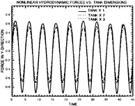
Figure 9: Hydrodynamic forces for surface-piercing cylinder versus tank dimensions.
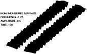
Figure 5: Nonlinear free surface evolution up to 20 cycles, NI=10, Δt=0.1.
ear free surface profiles corresponding to ω= 1.25 and A=0.5 through 20 cycles of oscillation. The nonlinear free surface tends to be more irregular than that predicted by linear theory. However, irregularities are not as pronounced as those reported by Yeung and Wu[ 46]. This is more easily seen in Figure 6 where grids at approximately 8.25, 8.5, 8.75 and 9th cycles are shown. Figure 7 shows velocity vector plots for the mesh points shown in Figure 6. It can be seen that good quality meshes and smooth velocity field distributions are obtained.
Figure 8 shows hydrodynamic heave forces for the conditions used in Figure 6. As pointed out by Yeung and Wu[46], for large oscillations, nonlinear theory predicts a larger negative peak and a smaller positive one with respect to the sinusoidal prediction of linear theory. This effect is essentially a consequence of the relative dimensions of the tank and the moving body. Figure 9 shows the effect of increasing the tank dimensions by 2 and 3 times while keeping the body dimensions constant. The resulting effect

Figure 6: Mesh deformation at 8.25, 8.5, 8.75 and 9th cycles.
is two-folded. First, a significant reduction of the amplitude of the hydrodynamic force is observed. Also, a decrease in the difference between positive and negative peaks of this force occurs.
6.2
Heave of submerged cylinder in a tank
Figure 10 shows a typical configuration for the mesh corresponding to the submerged cylinder. For this case, the cylinder radius is unity. The variable NI appearing in this section corresponds to the number of divisions used to discretize the free surface and a quarter of the body surface. Based on the experience gained in the case of the surface-piercing cylinder, in this section we have opted to use quadratic elements only. No smoothing was required for this case.
Figures 11 and 12 respectively show linear and nonlinear free surface time histories for A=0.5. Vertical dimensions have also been magnified by 10 times. Steeper peaks were observed

Figure 7: Velocity vector plots at 8.25, 8.5, 8.75 and pth cycles.

Figure 8: Hydrodynamic forces for surface-piercing cylinder.
to develop in the regions next to the tank walls for nonlinear results. Linear results predicted an almost sinusoidal behavior of the free surface across the width of the tank. As expected, vertical elevations remained lower than that obtained for the case of the surface-piercing cylinder.
Figure 13 shows mesh deformation corre-
Figure 10: Hydrodynamic forces for surface-peiercing cylinder versus tank dimensions.

Figure 10: Typical mesh for submerged cylinder.

Figure 11: Linear free surface for submerged cylinder (NI=20, Δt=0.1).

Figure 12: Nonlinear free surface time record for submerged cylinder (NI=10, t=0.05).
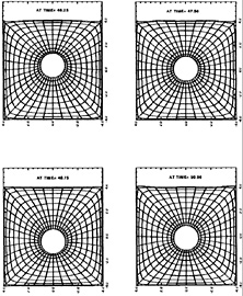
Figure 13: Mesh deformation at 9.25, 9.5, 9.75 and 10th cycles.
sponding to the 9.25, 9.5, 9.75 and 10th cycles of oscillation. Figure 14 shows corresponding velocity vector plots. Again, velocity fields behaved in a physically acceptable manner with very small differences between specified and calculated values.
For A=0.5, linear and nonlinear prediction of the hydrodynamic forces resulting from vertical motion of the circular cylinder displayed similar trends. Figure 15 shows linear and nonlinear hydrodynamic forces corresponding to an amplitude of motion A=1.5. Even for this extremely large amplitude of motion, both formulations gave similar results. Some differences

Figure 14: Velocity vector plots at 9.25, 9.5, 9.75 and 10th cycles.

Figure 15: Hydrodynamic force due to sinusoidal excitation, A=1.5.

Figure 16: Free surface frequency spectra due to impulsive motion for circular basin.
can again be seen in the force peaks, but these are significantly less noticeable than for the surface piercing case.
6.3
Impulsive motion in a tank
In this section, we present results corresponding to free surface response due to impulsive excitation of tanks of different shapes. Excitation is prescribed as a step velocity at t=0. We have opted to match the types of excitations given by Yeung and Wu[47]. Application of Fast Fourier Transform to the time record of the free surface elevation measured at a fixed point yields the frequency spectrum. Nondimensional frequencies for linear and nonlinear free surface boundary conditions are presented. Smoothing in the worst of these cases was applied using α=1 every 10th time step.
Figure 16 shows linear and nonlinear frequency spectra results for a circular tank. In this case, frequencies predicted by linear theory tend to be slightly higher than those given by nonlinear theory. Table 1 shows comparison with results given by Chang and Wu[70] (CW) using an integral equation formulation with linear boundary conditions. Their results also exhibit higher values than those predicted by nonlinear theory.
Corresponding results for a parabolic basin are given in Figure 17. For this particular configuration, results tend to show no difference be-
tween linear and nonlinear predictions. Table 2 compares our results with those given by Yeung and Wu[47]. In general, good agreement is achieved.
Table 1 Nondimensional frequencies for circular tank
|
CIRCULAR TANK |
|||
|
Freq. |
Lin. |
Nonl. |
CW |
|
1st |
1.7330 |
1.7180 |
1.7492 |
|
2nd |
2.4697 |
2.4545 |
2.5632 |
|
3rd |
3.0066 |
2.9759 |
— |
Table 2 Nondimensional frequencies for parabolic tank
|
PARABOLIC TANK |
||||
|
Freq. |
Lin. |
Nonl. |
YW. Lin. |
YW. Nonl |
|
1st |
1.6720 |
1.6720 |
1.6846 |
1.6846 |
|
2nd |
2.4390 |
2.4390 |
2.4170 |
2.4170 |
|
3rd |
3.0066 |
3.0066 |
3.0029 |
3.0029 |
Figure 18 shows results for a triangular basin. For this case, no definite trend is shown between linear and nonlinear results. As noted in Table 3, this effect is also shown in the results of Yeung and Wu[47]. Results by Lamb[71] are also presented.
Table 3 Nondimensional frequencies for triangular tank
|
TRIANGULAR TANK |
|||||
|
Freq. |
Lin. |
Nonl. |
YW. Lin. |
YW. Nonl |
Lamb |
|
1st |
1.5339 |
1.5646 |
1.5381 |
1.5381 |
1.5244 |
|
2nd |
2.3930 |
2.3930 |
2.3439 |
2.3438 |
2.3447 |
|
3rd |
3.0066 |
2.9912 |
2.9297 |
3.0029 |
2.9393 |

Figure 17: Free surface frequency spectra due to impulsive motion for parabolic basin.
6.4
Slender body calculations
In this section we present results corresponding to the forward motion of a mathematically defined ship hull advancing at zero angle of attack in otherwise calm water. The Wigley parabolic hull, whose main parameters are given in Table 4, is defined as
(19)
Table 4 Wigley hull dimensions
|
WIGLEY PARABOLIC HULL[m] |
|||||
|
Length L |
Beam B |
Draft D |
CB |
CWP |
CP |
|
2 |
0.2 |
0.125 |
0.444 |
0.667 |
0.667 |
Coordinates z and y remained as defined in pre-

Figure 18: Free surface frequency spectra due to impulsive motion for triangular basin.
vious sections for surface-piercing cases. The coordinate x is directed along the length of the hull and considered positive towards the stern.
Results presented for trim, sinkage and wave-resistance coefficients have been obtained for the conditions shown in Table 5. The tank width is in metres. The variable Δx refers to the spatial increment used along the x-coordinate in metres. For the length of the Wigley hull used in this study, this increment resulted in 2000 stations. CPU time estimates are presented in Table 6. Smoothing in the worst of these cases was also applied using α=1 every 10th time step.
Table 5 Computational conditions for Wigley hull calculations
|
COMPUTATIONAL CONDITIONS |
|||
|
Δx |
Tank Width |
No of elements |
No of Nodes |
|
0.001 |
3.0 |
1200 |
3741 |
Table 6 Computational demand for Wigley hull calculations
|
COMPUTATIONAL DEMANDS |
||
|
Machine Type |
Mflops |
CPU [min/Δx] |
|
SUN MP/670 |
4.0 |
5.0 |
|
IBM RS/6000 |
31.0 |
0.75 |
Figures 19 and 20 show linear and nonlinear three dimensional views of the free surface elevation for the Wigley hull advancing with a forward speed of ![]() . This corresponds with a length Froude number of 0.267. It is clear that nonlinear theory predicts a more realistic shape of the free surface. This is evident in the aft-half of the hull where linear theory is not able to produce the recovery from the second crest of the wave next to the hull. This is more easily seen in Figure 21 where comparison has been made with results presented by Maruo and Song[32]. Nonlinear results show good agreement with experimental values for the wave past the midship section. However, there is a shift of the first crest and trough of the fore-half of the wave. It is conjectured that one possible reason for this shift is due to the at rest (zero-valued) initial conditions used in this work. Figure 21 shows numerical results given by Maruo and Song[32] which clearly display non-homogeneous initial conditions. Free surface elevation contours are also shown in Figure 22 and Figure 23 for linear and nonlinear boundary conditions respectively. Nonlinear results show a ‘jagged' nature due to small wiggles appearing on the free surface. These wiggles were typical of nonlinear free surface profiles and occasionally were the origin of unstable behavior. In order to maintain the size of these wiggles bounded, small time steps (Δx) were used.
. This corresponds with a length Froude number of 0.267. It is clear that nonlinear theory predicts a more realistic shape of the free surface. This is evident in the aft-half of the hull where linear theory is not able to produce the recovery from the second crest of the wave next to the hull. This is more easily seen in Figure 21 where comparison has been made with results presented by Maruo and Song[32]. Nonlinear results show good agreement with experimental values for the wave past the midship section. However, there is a shift of the first crest and trough of the fore-half of the wave. It is conjectured that one possible reason for this shift is due to the at rest (zero-valued) initial conditions used in this work. Figure 21 shows numerical results given by Maruo and Song[32] which clearly display non-homogeneous initial conditions. Free surface elevation contours are also shown in Figure 22 and Figure 23 for linear and nonlinear boundary conditions respectively. Nonlinear results show a ‘jagged' nature due to small wiggles appearing on the free surface. These wiggles were typical of nonlinear free surface profiles and occasionally were the origin of unstable behavior. In order to maintain the size of these wiggles bounded, small time steps (Δx) were used.
Figure 24 shows the wave resistance coefficient as a function of the Froude number Fn for linear and nonlinear formulations. Data given by Aanesland[72] and mean values of experimental data from the 1st and 2nd Workshops on Wave Resistance Computations are presented [73,74]. At low values of Fn nonlinear prediction shows significant improvement over results

Figure 19: Linear free surface elevation for Wigley hull with forward speed, Fn=0.267.
obtained using linear theory. In fact, linear theory gives very poor agreement with experimental results for this Fn-range. For this set of experimental data, nonlinear results show superior performance throughout the Fn interval. Figure 25 shows the wave resistance coefficient compared with Maruo and Song[ 32]. Again, at low values of the Froude number nonlinear results give a better prediction than linear ones. However, as the Froude number increases, linear results show improvement over their nonlinear counterpart. This is a clear example of the scatter encountered in experimental data for these type of physical problems.
Figures 26 and 27 show sinkage and trim of the Wigley hull as a function of Fn. Improved predictions at the lower end of the Froude number interval used in this work are again realized for nonlinear results. This improvement is more clearly seen in the results for sinkage. These results suggest that nonlinear theory predicts a more accurate magnitude of the forces. This is consistent with results obtained for wave resistance as shown in Figure 24. Trim calculations show little discrepancy between linear and nonlinear results. In turn, this suggests that the distribution of forces is predicted with similar accuracy in both formulations.
CONCLUSIONS
The boundary value problem defined by the Laplace equation for the solution of potential

Figure 20: Non Linear free surface elevation for Wigley Hull with forward speed Fn=0.267

Figure 21: Wave profile at side of Wigley Hull with forward speed, Fn=0.267

Figure 22: Linear free surface elevation contours of Wigley hull with forward speed, Fn=0.267.

Figure 23: Nonlinear free surface elevation contours of Wigley Hull with forward speed, Fn=0.267
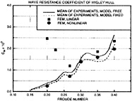
Figure 24: Wave resistace coefficient of Wigley hull versus Fn.

Figure 25: Wave resistance coefficient of Wigley hull versus Fn.

Figure 26: Sinkage of Wigley hull versus Fn.
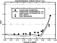
Figure 27: Trim of Wigley hull versus Fn.
flow in two dimensions has been formulated using a Bubnov-Galerkin weighted residual method to obtain the spatial variation of the velocity potential. The moving boundary problem corresponding to the a-priori unknown dependent and independent spatial variables in the nonlinear boundary conditions has been treated using a semi-Lagrangian semi-implicit scheme. This method proved to be more accurate and stable than predictor-corrector methods. When necessary, dissipation was applied only to the velocity potential.
ACKNOWLEDGEMENT
I (AA) would like to extend my sincere gratitude to Dr. Rodolfo Bermejo for his generous assistance during the development of some of the concepts expressed in this paper. I am also thankful to Dr. Chun-Fa Wu for his help during our phone conversations.
REFERENCES
[1] Van Dyke M.D., ‘Perturbation Methods in Fluid Mechanics', Academic Press, 1964.
[2] Cummins W.E., ‘The Wave Resistance of a Floating Slender Body', Unpublished Thesis, American University, 1956.
[3] Kaplan P., ‘Application of Slender Body Theory to Forces Acting on Submerged Bodies and Surface Ships in Regular Waves', Journal of Ship Research, vol. 1, 1957.
[4] Lighthill M.J., ‘Note on the Swimming of Slender Fish', Journal of Fluid Mechanics, vol. 9, 1960.
[5] Vossers G., ‘Wave Resistance of a Slender Ship', Schiffstechnik, vol. 9, 1962.
[6] Maruo H., ‘Calculation of the Wave Resistance of Ships, the draft of which is as small as the beam', Journal of the Society of Naval Architects of Japan, vol. 112 , 1962.
[7] Ursell F., ‘Slender Oscillating Ships At Zero Forward Speed', Journal of Fluid Mechanics, vol. 14, 1962.
[8] Tuck E.O., ‘A Systematic Asymptotic Expansion Procedure for Slender Ships', Journal of Ship Research, vol. 8, 1964.
[9] Newman J.N. and Tuck E.O., ‘Current Progress in the Slender Body Theory for Ship Motions', Procceedings of the 5th Symposium on Naval Hydrodyanmics, 1964.
[10] Newman J.N., ‘The exciting Forces on a Moving Body in Waves', Journal of Ship Research, vol. 9, 1965.
[11] Haskind M.D., ‘The exciting Forces and Wetting of a Ship in Waves', Izvestia Akademii Nauk SSSR, 1957 (in russian). DTMB translation No 307, 1962.
[12] Tuck E.O., ‘Shallow-Water Flows Past Slender Bodies', Journal of Fluid Mechanics, vol. 26, 1966.
[13] Newman J.N., ‘Applications of Slender Body Theory in Ship Hydrodynamics', Annual Review of Fluid Mechanics, vol. 2, 1970.
[14] Chapman R.B., ‘Free Surface Effects for Yawed Surface Piercing Plates', Journal of Ship Research, vol. 20 , 1976.
[15] Jensen J.J. and Pedersen P.T., ‘Wave-Induced Bending Moments in Ships', Transactions of the Royal Institute of Naval Architects, vol. 121 , 1979.
[16] Troesch A.W., ‘Sway, Roll and Yaw Motion Coefficients Based on a Forward Speed Slender Body Theory: Part 1', Journal of Ship Research, vol. 25, 1981.
[17] Troesch A.W., ‘Sway, Roll and Yaw Motion Coefficients Based on a Forward Speed Slender Body Theory: Part 2', Journal of Ship Research, vol. 25, 1981.
[18] Maruo H., ‘New Approach to the Theory of Slender Ships with Forward Speed', Bulletin of the Faculty of Engineering, Yokohama University, vol. 31, 1982.
[19] Noblesse F., ‘A Slender Ship Theory of Wave Resistance', Journal of Ship Research, vol. 27, 1983.
[20] Faltinsen O.M., ‘Bow Flow and Added Resistance of Slender Ships at High Froude Numbers and Low Wave Lengths', Journal of Ship Research, vol. 27, 1983.
[21] Chen C.Y. and Noblesse F., ‘Preliminary Numerical Study of a New Slender Ship Theory of Wave Resistance', Journal of Ship Research, vol. 27, 1983.
[22] Chen C.Y. and Noblesse F., ‘Comparison Between Theoretical Predictions of Wave Resistance and Experimental Data for the Wigley Hull', Journal of Ship Research, vol. 27, 1983.
[23] Sclavounos P.D., ‘The Diffraction of Free Surface Waves by a Slender Ship', Journal of Ship Research, vol. 28, 1984.
[24] Sclavounos P.D., ‘The Unified Slender Body Theory: Ship Motions in Waves', Proceedings of the 15th Symposium on Naval Hydrodynamics, 1984.
[25] Breit S.R. and Sclavounos P.D., ‘Wave Interactions Between Adjacent Slender Bodies', Journal of Fluid Mechanics, vol. 165, 1986.
[26] Song W., Ikehata M. and Suzuki K., ‘Computation of Wave Resistance and Ship Wave Pattern by the Slender Body Approximation', Journal of the Kamsai Society of Naval Architects of Japan, vol. 209, 1988, in Japanese.
[27] Choi H.S. and Mei C.C., ‘Wave Resistance
and Squat of a Slender Ship Moving Near the Critical Speed in Restricted Waters', Proceedings of the 5th International Conference on Numerical Ship Hydrodynamics, 1989.
[28] Kashiwagi M., ‘Theoretical prediction of Tank Wall Effects on Hydrodynamic Forces Acting on an Oscillating and Translating Slender Ship', Extended Abstracts of the 4th International Workshop on Water Waves and Floating Bodies, 1989.
[29] Kashiwagi M., ‘Side Wall Effects on Hydrodynamic Forces Acting on a Ship with Forward and Oscillating Motions', Proceedings of the 5th International Conference on Numerical Ship Hydrodynamics, 1989.
[30] Calisal S.M. and Chan J.L.K., ‘A Numerical Model of Ship Bow Waves', Journal of Ship Research, vol. 33, 1989.
[31] Ando S., ‘Forward Speed Effect in Head Wave Diffraction over the Forebody of A Slender Hull', Extended Abstracts of the 4th International Workshop on Water Waves and Floating Bodies, 1989.
[32] Maruo H. and Song W., ‘A Numerical Appraisal of the New Slender Ship Formulation in Steady Motion', Proceedings of the 18th Symposium on Naval Hydrodynamics, 1990.
[33] Yeung R.W., ‘Numerical Methods in Free Surface Flows', Annual Review of Fluid Mechanics, vol. 14, 1982.
[34] Longuet-Higgins M.S. and Cokelet E.D., ‘The Deformation of Steep Surface Waves on Water I: A Numerical Method of Computation'. Proceedings of the Royal Society of London, Series A 350, 1976.
[35] Vinje T. and Brevig P., ‘Nonlinear Ship Motion', Proceedings of the 3rd International Conference on Numerical Ship Hydrodynamics , 1981.
[36] Lin W.M, Newman J.N. and Yue D.K., ‘Nonlinear Forced Motions of Floating Bodies', Proceedings of the 15th International Symposium on Naval Hydrodynamics , 1985.
[37] Baker G.R., Meiron D.J. and Orzag S.A., ‘Generalized Vortex Methods for Free-Surface Flow Problems', Journal of Fluid Mechanics, vol. 123, 1982.
[38] Dold J.W. and Peregrine D.H., ‘Steep Unsteady Water Waves: An Efficient Computational Scheme', Proceedings of the 19th International Conference on Coastal Engineering, ASCE, 1984.
[39] Suzuki K., ‘Calculation of Nonlinear Water Waves Around a Two-Dimensional Body in Uniform Flow by Means of a Boundary Element Method', Proceedings of the 5th International Conference on Numerical Ship Hydrodynamics, 1989.
[40] Sen, D., Pawlowsky J.S., Lever J. and Hinchey M.J., ‘Two-Dimensional Numerical Modelling of Large Motions of Floating Bodies in Waves', Proceedings of the 5th International Conference on Numerical Ship Hydrodynamics, 1989.
[41] Cointe R., ‘Nonlinear Simulation of Transient Free Surface Flows', Proceedings of the 5th International Conference on Numerical Ship Hydrodynamics, 1989.
[42] Cointe R., Geyer P., King B., Molin B. and Tramoni M., ‘Nonlinear and Linear Motions of a Rectangular Barge in a Perfect Fluid', Proceedings of the 18th International Symposium on Naval Hydrodynamics , 1990.
[43] Ghia U., Shin C.T. and Ghia K.N., ‘Analysis of a Breaking Free Surface Wave Using Boundary Fitted Coordinates for Regions Including Reentrant Boundaries', Proceedings of the 3rd International Conference on Numerical Ship Hydrodynamics, 1981.
[44] Haussling A.J., ‘Solution of Nonlinear Water Wave Problems Using Boundary Fitted Coordinate Systems', Numerical Grid Generation: J.Thompson, editor, 1982.
[45] Telste J.G., ‘Calculation of Fluid Motion from Large-Amplitude Forced Heave Motion of a Two-Dimensional Cylinder in a Free Surface', Proceedings of the 4th International Conference on Numerical Ship Hydrodynamics, 1985.
[46] Yeung R.W. and Wu C., ‘Nonlinear Wave-Body Motion in a Closed Domain', Computers & Fluids, vol. 17, 1989.
[47] Yeung R.W. and Wu C. , ‘On Nonlinear Wave Motion in a Closed Domain', Jahrbuch
der Schiffbautechnischen Gesellschaft, vol. 83, 1989.
[48] Luke J.C., ‘A Variational Principle for a Fluid with a Free Surface', Journal of Fluid Mechanics, vol. 27, 1967.
[49] Whitman G.B., ‘Nonlinear Dispersion of Water Waves', Journal of Fluid Mechanics, vol. 27, 1967.
[50] Whitman G.B., ‘Two-timing, Variational Principles and Waves', Journal of Fluid Mechanics, vol. 44, 1970.
[51] K.J.Bai and R.W.Yeung, ‘Numerical Solutions to Free Surface Flow Problems', Proceedings of the 10th Symposium on Naval Hydrodynamics, 1974.
[52] Bai K.J., ‘Diffraction of Oblique Waves by an Infinite Cylinder', Journal of Fluid Mechanics, vol. 68, 1975.
[53] Yim B., ‘A Variational Principle Associated with a Localized Finite Element Technique for Steady Ship-Wave and Cavity Problems', Proceedings of the 1st International Conference on Numerical Ship Hydrodynamics, 1975.
[54] Bai K.J., ‘A Localized Finite Element Method for Steady, Two Dimensional Free Surface Flow Problems', Proceedings of the 1st International Conference on Numerical Ship Hydrodynamics, 1975.
[55] Bai K.J., ‘A Localized Finite Element Method for Two-Dimensional Steady Potential Flows with a Free Surface', Journal of Ship Research, vol. 22, 1978.
[56] Bai K.J., ‘Blockage Correction with a Free Surface', Journal of Fluid Mechanics, vol. 94, 1979.
[57] Wellford C.L. and Ganaba T., ‘Finite Element Procedures for Fluid Mechanics Problems Involving Large Free Surface Motion', Proceedings of the 3rd International Conference in Finite Elements in Flow Problems, 1980.
[58] Oomen A., ‘Free Surface Potential Flow Computation Using a Finite Element Method ', Proceedings of the 3rd International Conference on Numerical Ship Hydrodynamics, 1981.
[59] Jami A., ‘Numerical Solving of Transient Linear Hydrodynamics Problems by Coupling Finite Elements and Integral Representation', Proceedings of the 3rd International Conference on Numerical Ship Hydrodynamics, 1981.
[60] Euvard D., Jami A., Lenoir M. and Martin D., ‘Recent Progress Towards an Optimal Coupling between Finite Elements and Singularity Distribution Procedures', Proceedings of the 3rd International Conference on Numerical Ship Hydrodynamics, 1981.
[61] Allievi A. and Calisal S.M., ‘Finite Element Application to Grid Generation for Submerged and Floating Bodies', International Symposium on Hydro & Aero Dynamics In Marine Engineering, 1991.
[62] Allievi A. and Calisal S.M., ‘A Bubnov-Galerkin Formulation For Orthogonal Grid Generation', Journal of Computational Physics, vol. 98, 1992.
[63] Allievi A., ‘On Nonlinear Free Surface Potential Flow by a Bubnov-Galerkin Formulation in Space and a Semi-Lagrangian Semi-implicit scheme in Time', Ph.D. thesis, University of British Columbia, in preparation.
[64] Robert A.J., ‘A Stable Numerical Integration Scheme for the Primitive Meteorological Equations', Atmosphere-Ocean, vol. 19, 1981.
[65] Robert A.J., ‘A Semi-Lagrangian and Semi-Implicit Numerical Integration Scheme for the Primitive Meteorological Equations', Journal of the Meteorological Society of Japan, vol. 60, 1982.
[66] Staniforth A. and Temperton C., ‘Semi-Implicit Semi-Lagrangian Integration Schemes for a Barotropic Finite-Element Regional Model', Monthly Weather Review, vol. 114, 1986.
[67] Staniforth A. and Temperton C., ‘An Efficient Two-Time-Level Semi-Lagrangian Semi-Implicit Integration Scheme', Quarterly Journal of the Royal Meteorological Society, vol. 113, 1987.
[68] Bermejo R., ‘An Analysis of an Algorithm for the Galerkin-Characteristic Method ', Numerische Mathematik, vol. 60, 1991.
[69] Ryskin G. and Leal L.G., ‘Orthogonal Map-
ping', Journal of Computational Physics, vol. 50, 1983.
[70] Chang S.C. and Wu S.T., ‘On the Natural Frequencies of Standing Waves in a Canal of Arbitrary Shape', Journal of Applied Mathematics and Physics, vol. 23, 1972.
[71] Lamb H., ‘Hydrodynamics', Cambridge University Press, 1932.
[72] Aanesland V., ‘A Hybrid Model for Calculating Wave Making Resistance', Proceedings of the 5th International Conference on Numerical Ship Hydrodynamics, 1989.
[73] ‘Proceedings of the First Workshop on Ship Wave Resistance Computations ', David Taylor Naval Ship Research and Development Center, 1979.
[74] ‘Proceedings of the Second Workshop on Ship Wave Resistance Computations ', David Taylor Naval Ship Research and Development Center, 1983.


