
Numerical Analysis of Nonlinear Ship Wavemaking Problem by the Coupled Element Method
X.W.Yu,1 S.M.Li,2 and C.C.Hsiung1
(1Technical University of Nova Scotia, Canada, 2Wuhan University of Water Transportation Engineering, PRC)
Abstract
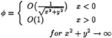
In this paper, the free surface condition for the ship wavemaking problem is analyzed and simplified with a new order analysis for the ship wavemaking potential based on the slow-ship theory. The total velocity potential is expressed as Φ=x+φr+φ, where φ is the wave disturbance potential, and φr is the double-body disturbance potential with the order ![]() and k>1, so that the nonlinear free surface condition can be simplified and calculated on z=0. In the numerical calculation, the coupled element method is applied. The flow domain is divided into inner and outer regions. The finite element method is used with the simplified nonlinear free surface condition for the inner region and the Green function method is employed with the linear free surface condition for the outer region. In the outer region, the Kelvin source function is used as the Green function, so that no numerical treatment of the radiation condition is needed. Numerical calculations were carried out for a cylinder, a sphere, a Wigly model and a Series 60 Block 60 ship model. The computed results agree well with the experimental results.
and k>1, so that the nonlinear free surface condition can be simplified and calculated on z=0. In the numerical calculation, the coupled element method is applied. The flow domain is divided into inner and outer regions. The finite element method is used with the simplified nonlinear free surface condition for the inner region and the Green function method is employed with the linear free surface condition for the outer region. In the outer region, the Kelvin source function is used as the Green function, so that no numerical treatment of the radiation condition is needed. Numerical calculations were carried out for a cylinder, a sphere, a Wigly model and a Series 60 Block 60 ship model. The computed results agree well with the experimental results.
Nomenclature
|
a |
: radius of a cylinder or a sphere |
|
A,B,C,D,E,F,H,P,Q,R,S,U,V,W |
: order groups or coefficient matrices |
|
CB |
: block coefficient |
|
CL |
: lift coefficient |
|
Cw |
: wave resistance coefficient |
|
Cx |
: midship section coefficient |
|
Cs |
: wetted surface area coefficient |
|
D |
: flow domain |
|
D1 |
: inner region of the flow domain |
|
D2 |
: outer region of the flow domain |
|
Fn |
: Froude number |
|
g |
: gravitational acceleration |
|
G |
: Green's function |
|
L,B,T |
: ship length, beam, and draft, respectively |
|
LB |
: intersection of ship hull and free surface |
|
L1,L2,L3 |
: path of the line integral |
|
|
: unit outer normal vector |
|
N |
: total number of nodes |
|
Ni |
: shape function |
|
p |
: pressure |
|
Rw,L |
: wave resistance and lift on a body, respectively |
|
SB |
: wetted surface of ship |
|
S1 |
: boundary of the inner region |
|
S2 |
: boundary of the outer region |
|
SF1 |
: free surface of the inner region |
|
SF2 |
: free surface of the outer region |
|
Sj |
: interface of the inner and outer regions |
|
S∞ |
: boundary surface at infinity |
|
U |
: ship speed |
|
x,y,z |
: Cartesian coordinate system |
|
α |
: solid angle at a control point |
|
η |
: wave elevation |
|
Φ |
: total velocity potential |
|
|
: disturbance potential |
|
φ |
: wave disturbance potential |
|
φr |
: double-body disturbance potential |
|
ρ |
: fluid density |
1
Introduction
Normally, ship wavemaking is a highly nonlinear problem. The major difficulty in this problem lies in the nonlinear boundary condition at the unknown location of the free surface. A basic approach to deal with this nonlinear problem is to employ the perturbation analysis. Almost exclusively a linearized condition is applied at the free surface, and in most cases the solution is described by a superposition of complicated singularities that satisfy this linearized free surface condition. Based on the assumption of small Froude number the low-speed ship theory, which takes account of the nonlinear effect on the free surface condition, has been developed. The perturbation process was applied to the zero-Froude number flow field instead of the free stream. The series expansion with respect to the wave elevation was carried out. The small parameter of Froude number was introduced to simplify the nonlinear free surface condition. This perturbation analysis with a quasi-analytic method, which was developed by Baba [1] for the low-speed flow past a blunt ship bow, gave a good agreement of computed and experimental results of wave-resistance coefficient over a range of low Froude numbers. Based on the same perturbation method, in 1977, Dawson[2] developed a numerical method by distributing the Rankine sources on the body surface and on the local free surface around the body. A wave field was superimposed on the double-body flow. The source strength distribution on the body surface and on the local free surface was obtained by satisfying the body boundary condition and the free surface condition. The radiation condition, which states that the ship waves occur only behind the ship, was replaced by a one-side finite difference operator for the second derivative of the potential in the direction of the double-body streamlines appearing in Dawson 's free surface boundary condition. Good numerical results were obtained by Dawson's method despite the fact that the numerical treatment of the radiation condition has no theoretical support.
The finite element method is known to be flexible for the nonlinear problem and for the boundary value problem with a complicated boundary. Therefore many researchers have developed numerical methods based on the finite element method to solve the free surface flow problems. Bai[3] developed the localized finite element method for calculating wave resistance of a body moving in a channel. Recently Bai and others [4] successfully used the finite element method to solve the nonlinear wavemaking problem in shallow water, but his method was not applied to the infinite domain. Eatok-Taylor and Wu[5] used the coupled element method to calculate wave resistance and lift on 2-D submerged cylinders, but did not cover the 3-D ship wavemaking problem.
In this work, a new order analysis of the wavemaking potential is developed. As a result, a simplified free surface condition, which takes account of the effect of nonlinearity but is different from Dawson's free surface condition, is obtained. The coupled element method is employed to solve the 3-D ship wavemaking problem. In the numerical computation, the flow domain is divided into two regions as shown in Fig.1: the inner region originates around the ship hull and is bounded by surfaces Sj+SB+SF1; the outer region is outside the interface Sj and is bounded by surfaces Sj+SF2+S∞. In the inner region the effect of nonlinearity of the free surface is very important, so that the finite element method is used together with the simplified nonlinear free surface condition. The effect of nonlinearity is negligible in the outer region far from the ship hull, where the Green function method is employed with the linear free surface condition. The Kelvin source function is adopted as the Green function, consequently, the radiation condition is satisfied exactly. By matching the solutions of the inner and outer regions at the interface of two regions, the solution for the entire flow field can be found. Numerical computations have been carried out for a submerged cylinder, a submerged sphere, a Wigly model and also a Series 60 Block 60 ship model. The computed results agree well with the experimental results.
2
The Free Surface Condition
2.1
Exact Mathematical Expression for the Wavemaking Potential
The coordinate system and flow domain are shown in Fig. 1. It is assumed that the fluid is ideal and incompressible, and the flow is irrotational and steady. The Froude number is defined by ![]() , where U is the ship speed, g the gravitational constant and L the ship length. The
, where U is the ship speed, g the gravitational constant and L the ship length. The
total velocity potential is written as
(1)
in which ![]() must satisfy the Laplace equation
must satisfy the Laplace equation
![]() in domain D (2)
in domain D (2)
subject to the following boundary conditions:
on the free surface η(x,y) (3)
on the free surface η(x,y) (4)
on the body surface SB (5)
(6)
The problem described by (2)—(6) is the exact mathematical representation of the boundary value problem of the ship wavemaking potential.
2.2
Simplification of the Free Surface Condition
The ship wavemaking problem described by (2)–(6) is a highly nonlinear problem. As well-known, the difficulty lies in that the free surface condition is nonlinear and must be satisfied on the unknown surface. Before trying to solve the nonlinear problem, we have to simplify the free surface condition. It is assumed that the Froude number, Fn, is sufficiently small.
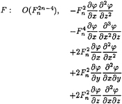
By substituting (3) into (4) and keeping the terms of the products of derivatives of ![]()
(7)
after applying Taylor's expansion to the wave elevation and again keeping the products of derivatives of ![]() , we obtain
, we obtain
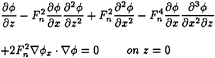
(8)
The disturbance potential ![]() can be further decomposed into two parts,
can be further decomposed into two parts,
(9)
where φr denotes the double body disturbance potential and φ the wave disturbance potential.
If we assume that:
(1) ![]()
for φr, i=1, 2, 3
(2) ![]()
for φ, i=1, 2, 3
Substituting (9) into (8), we obtain
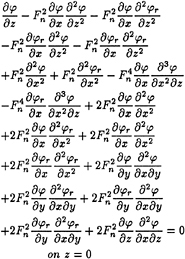
(10)
If (10) is classified according to the following orders

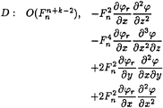

From above, these different groups generally differ from one another with their orders of magnitude. It is clear that:
1. for the terms with the wave potential φ, no matter what value n is, the following is always true:
n−2<n+k−2<n+k
which means that group D is smaller than group A by ![]() , and group E is smaller than group D by
, and group E is smaller than group D by ![]()
2. for the terms only including the double-body disturbance potential, no matter what value k is, the following always exists
k+2<2k+2
which means that group C is smaller than group B by ![]()
The order of magnitude of each group with the difference between n and k is shown in Table 1.
Table 1 The order of magnitude with the difference between n and k
|
GROUP |
ORDER |
n=k+5 |
n=k+4 |
n=k+3 |
n=k+2 |
|
A |
n−2 |
k+3 |
k+2 |
k+1 |
k |
|
B |
k+2 |
k+2 |
k+2 |
k+2 |
k+2 |
|
C |
2k+2 |
2k+2 |
2k+2 |
2k+2 |
2k+2 |
|
D |
n+k−2 |
2k+3 |
2k+2 |
2k+1 |
2k |
|
E |
n+k |
2k+5 |
2k+4 |
2k+3 |
2k+2 |
|
F |
2n−4 |
2k+6 |
2k+4 |
2k+2 |
2k |
From Table 1, it can be seen that:
-
Group E is the first one to be neglected.
-
With a decrease of the difference between n and k, group F becomes more influential and group C becomes less influential.
-
In addition to groups A and B, the first group to be considered is group D.
-
The value of k has no effect on the choice of the terms in the free surface condition.
The difference between n and k represents the magnitude of the wave potential. The large difference shows the small effect of wave potential, and the small difference means that large wave has been made by the ship at high speed. Since we assume that the ship speed is low, the small difference will lead to invalidation of the assumption, therefore in the numerical calculation we only keep groups A, B, C and D in the free surface condition:
(11)
If only the group A is kept in the free surface condition, the well-known linear free surface condition is obtained:
(12)
3
The Coupled Element Method for the Ship Wavemaking Problem
In the boundary value problem of ship wavemaking, the wave disturbance potential should satisfy:
∇2φ=0 z≤0 (13)
![]() z=0 (14)
z=0 (14)
![]() on SB (15)
on SB (15)

(16)
where for the linear ship wavemaking problem, ![]() , f2(x,y,z)=−nx; and for the nonlinear problem, it is easy to obtain f1(x,y) from (11), and f2(x,y,z)=0.
, f2(x,y,z)=−nx; and for the nonlinear problem, it is easy to obtain f1(x,y) from (11), and f2(x,y,z)=0.
As mentioned before, for numerical calculation, the flow domain is divided into two regions. In the inner region around the ship hull, the finite element method is used to solve the nonlinear problem; whereas, the effect of nonlinearity is negligible in the outer region far from the ship hull, thus the Green function method is adopted to solve the linear problem. By matching the solutions of inner and outer regions at their interface, the solution for the entire flow field can be obtained.
The flow domain is shown in Fig. 1. D1, with the boundary S1=SB+SF1+Sj, represents the inner region where the wave potential is defined by φ1. D2, with the boundary S2=Sj+SF2+S∞, represents the outer region where the wave potential is defined by φ2. On Sj, the interface of two regions, φ1 and φ2 should satisfy the matching conditions:
φ1=φ2on Sj (17)
![]() on Sj (18)
on Sj (18)
3.1
The Green Function Method for φ2 in the Outer Region
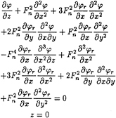
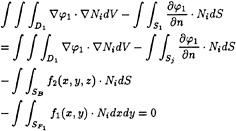
In the outer region D2, the linear free surface condition (12) is used. Applying the Green function method to the potential φ2 in D2 gives
(19)
Using the matching conditions (17) and (18), on the surface Sj, we obtain

(20)
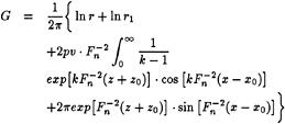
where α is the solid angle at the control point p on Sj and G is the Kelvin source function[8]

(21)
If φ1 and ![]() in D1 are now approximated by
in D1 are now approximated by
(22)
(23)
where Ni is the so-called shape function. If the problem we deal with is a Neumann-Kelvin problem of a submerged body, we can choose the inner region under the free surface, then the line integral on the line L1+L2 will disappear. Eq. (20) can be simply rewritten in a discretized form
(24)
or, identically,
(25)
where the element of [A] is
(26)
the element of [B] is
(27)
In a general case, the line integral on L1+L2 exists, then Eq.(20) can not be written as (24). We have to pay special attention to the treatment of the line integral.
3.2 Auxiliary Equations for Computing the Line Integral on the Free Surface
When the boundary of the inner region D1 includes the free surface SF1, the line integral on L1+L2 exists(please see Fig. 1). Since the Kelvin source function is not defined on the free surface when control points are the nodes on the L1+ L2, the Kelvin sources cannot be distributed on these points. After discretization, the number of equations is not equal to the number of nodes on the interface Sj, then the linear equation system is not in a closed form. It can be expressed by the following matrix form
(28)
where [φ1] is the unknown potential vector at the nodes on the surface Sj under the free surface, and [φ10] is the unknown potential vector at the nodes on the path of the line integral. [D] and [F] are the coefficient matrices including the contribution from both surface integrals and line integrals on the interface elements, [E] and [H] are the coefficient matrices only related to line integrals on L1+L2.
Since the system equation expressed by Eq.(28) is not in a closed form, we have to establish auxiliary equations from the relationship between φ1 and ![]() on L1+L2. The potential φ1 has to satisfy the following conditions: φ1 is continuous in D1, and the continuity is extended to the boundary of D1; in addition, φ1 has to satisfy the Laplace equation and the free surface condition.
on L1+L2. The potential φ1 has to satisfy the following conditions: φ1 is continuous in D1, and the continuity is extended to the boundary of D1; in addition, φ1 has to satisfy the Laplace equation and the free surface condition.
By the finite element approach, we can write
(29)
(30)
then we have
(31)
For example, on L2, we have
(32)
(33)
In the outer region D2, we have the linear free surface condition:
After discretization, we can write the matrix form
(34)
combining (28) and (34), we get
(35)
we can also write (35) as
(36)
where

where N is the total number of nodes on the Sj, and M is the total number of nodes on the elements only along the line integral path plus the total number of nodes on the Sj.
3.3 The Finite Element Method for φ1 in D1
According to the Galerkin method, for every Ni, φ1(x,y,z) has to satisfy
(37)
By the Green thoerom, it is clear that
(38)
where S1=Sj+SB+SF1.
(38) becomes
(39)
a. the Neumann-Kelvin problem
For the Neumann-Kelvin problem
(40)
f2(x,y,z)=−nx (41)
(39) becomes

(42)
From (36),
(43)
(44)
Substituting (43) and (44) into (42), we write (42) as a matrix form
[U+V][φ1]=[W] (45)
where the elements of [U] are

(46)
The matrix [V] expresses the matching conditions. Its elements are

(47)
[W] is the known vector,
(48)
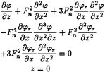
b. the nonlinear problem
For the nonlinear problem, refer to Eq.(11) and Eq.(14)
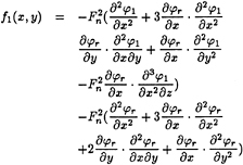
(49)
For Eq.(15)
f2(x,y,z)=0 (50)
Similarly as (45), for the nonlinear problem we can also obtain
[U+V][φ1]=[W] (51)
where

(52)

(53)
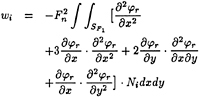
(54)
By solving (51) we can obtain φ1 for the inner region.
4 Numerical Results
The numerical calculations have been carried out for wave resistance of a 2-D submerged cylinder, a 3-D submerged sphere, a Wigly model and a Series 60 Block 60 model.
From the Bernoulli integral
(55)
for the nonlinear problem, ![]() =φr +φ1.
=φr +φ1.
The wave resistance and lift are calculated by integrating pressure over the wetted body surface.
(56)
(57)
4.1 The Submerged Cylinder
For a submerged cylinder the wave resistance and lift have been calculated by the coupled element method. The inner region D1 was discretized with 8-node isoparameter quadrilateral elements. The nonlinear free surface condition is
(58)
and the 2-D Green function[8] for the outer region is
(59)
where
r=[(x−x0)2+(z−z0)2]½
r1=[(x−x0)2+(z+z0)2]½
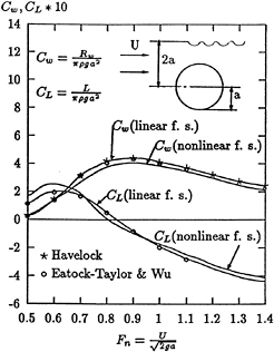
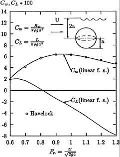
The computed results are compared with results from Havelock's analytical solution and Eatock-Taylor and Wu's numerical results as shown in Fig.3. For the Neumann-Kelvin problem, our numerical results agree very well with the referred results. The solution with the nonlinear free surface condition is not too different from the solution with the linear free surface condition.
4.2 The Submerged Sphere
Using the coupled element method, the Neumann-Kelvin problem has been solved for a submerged sphere. The inner region D1 was under the free surface. 20-node isoparameter hexagon elements were used to discretize the inner region. The comparison between the numerical result and Havelock's analytical solution is shown in Fig. 4. They agree very well.
4.3 Wigly Ship Model
The Wigly ship hull of mathematical form is expressed by
(60)
where
with
CB=0.444 CP=0.667
Cx=0.667 Cs=0.661
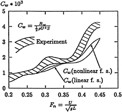
The numerical results for the wave resistance coefficient are compared with the experimental results, shown in Fig. 5. Comparing with the solution with the linear free surface condition, the numerical solution with the simplified nonlinear free surface condition is more agreeable with the experimental results.
4.4 Series 60 Block 60 Ship Model
In the numerical calculation, the inner region D1 is chosen as −1.25L≤x≤1.25L, 0≤y≤ 0.5L and −0.06L≤z≤0. We discretized D1 into 120 quadratic isoparameter hexahedron elements with 819 nodes. The computed wave resistance coefficient curves are compared with other known results, shown in Fig. 6.
5 Discussion and Concluding Remarks
In the present study, based on the low-speed ship theory, an investigation has been made into the free surface conditions. Through a new approach of the order analysis, a simplified nonlinear free surface condition, which is different from Baba's and Dawson's, has been obtained.
The coupled element method has been introduced for numerical calculation. Efforts have been made for the treatment of the line integral along L1+L2 (Fig. 1). Auxiliary equations on the path L1+L2 of the line integral were established by using the free surface and continuity conditions to overcome the difficulty arisen in computing the line integral. Also, by using the Kelvin source function as the Green function in the outer
region, no numerical treatment of the radiation condition is needed.
In the finite element method, the form of the shape function and the element dimension have an important effect on the numerical result. The quadratic isoparameter hexahedron elements were used to discretize the inner region in order to match the ship hull geometry. The element dimension has a direct effect on the computer time, storage of data and solution accuracy. Before using the coupled element method to the ship wavemaking problem, a special investigation was carried out to find the effect of the element dimension on the numerical results. Wave resistance and lift coefficients of a submerged sphere have been computed for different values of maximum element dimension Lm/(U2/g). They are shown in Table 2.
Table 2
|
Lm/(U2/g) |
Cw |
CL |
|
0.5 |
0.06210 |
−0.02910 |
|
1.0 |
0.06190 |
−0.02915 |
|
1.5 |
0.06195 |
−0.02920 |
|
2.5 |
0.06220 |
−0.02930 |
|
3.0 |
0.06230 |
−0.02950 |
|
3.5 |
0.06450 |
−0.03130 |
From Table 2, it is suggested to keep Lm/(U2/g) within the limit of 1.0 ~ 3.0 for calculations.
Computations were carried out on Silicon Graphics IRIS 4D/120SX. The CPU time for computing the wave resistance coefficient for one Froude number on the Series 60 Block 60 model is about 28 minutes. For this numerical calculation, the inner region D1 was discretized into 120 quadratic isoparameter hexahedron elements with 819 nodes, and the interface Sj was represented by 96 quadratic isoparameter quadrilateral elements with 329 nodes. Most of the computer time was consumed on computation of coefficient matrices A and B in Eq.(36) which is related to integrals of the Kelvin source function and its derivatives on quadrilateral elements. The calculation method was mainly based on Shen and Farell 's work[9]. The four-point Gaussian quadrature was employed for computing the surface integrals. The nine-point Gaussian quadrature was also applied. It increased the computing time by almost twice for one Froude number but did not improve the computing results significantly, only varied about 3 to 4%. The computed results of the Series 60 Block 60 model agree well with the experimental results.
Acknowledgements
This work was originally developed at the Wuhan University of Water Transportation Engineering under the support of Chinese Natural Science Foundation. Part of this work was recomputed at the Technical University of Nova Scotia under the support of the Natural Sciences and Engineering Council of Canada.
References
1. Baba, E., and Hara, M., “Numerical Evaluation of Wave-Resistance Theory for Slow Ships,” Second International Conference on Numerical Ship Hydrodynamics, Sept. 1977, PP. 17– 29.
2. Dawson, C.W., “A Practical Computer Method for Solving Ship Wave Problem,” Second International Conference on Numerical Ship Hydrodynamics, Sept. 1977, pp. 30–38.
3. Bai, K.J., “A localized Finite Element Method for Steady Three-Dimensional Free-Surface Flow Problem,” Second International Conference on Numerical Ship Hydrodynamics, Sept. 1977, pp. 78–87.
4. Choi, H.S., Bai, K.J., Kim, J.W., and Cho, I.H., “Nonlinear Free Surface Waves Due to a Ship Moving Near the Critical Speed in a Shallow Water,” Eighteenth Symposium on Naval Hydrodynamics, 1991, pp. 173–190.
5. Eatock-Taylor, R., and Wu, G.X., “Wave Resistance and Lift on Cylinders By Coupled Element Technique, ” International Ship Progress, Vol.33, 1986
6. Raven, H., “Adequacy of Free Surface Conditions for the Wave Resistance Problem, ” Eighteenth Symposium on Naval Hydrodynamics, 1991, pp. 375– 396.
7. Aanesland, V., “A Hybrid Model for Calculating Wave-Making Resistance,” Fifth International Conference on Numerical Ship Hydrodynamics, Sept. 1989, pp. 657–666.
8. Wehausen, J.V., and Laitone, E.V., “Surface Waves,” Handbuch der Physik, Vol.9, 1960
9. Shen, H.T., and Farell, C., “Numerical Calculation of the Wave Integrals in the Linearized Theory of Water Waves,” Journal of Ship Research, Vol.21, No.1, 1977, pp. 1–10.
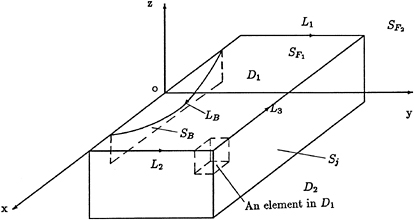
Fig.1 Coordinate System and Flow Domain
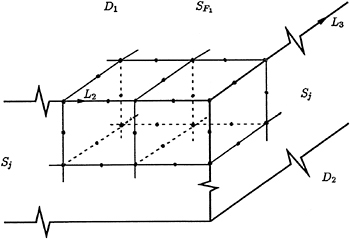
Fig.2 Finite Elements in D 1

Seakeeping and Wave Induced Loads on Ships with Flare by a Rankine Panel Method
P.D.Sclavounos, D.E.Nakos, and Y.Huang
(Massachusetts Institute of Technology, USA)
ABSTRACT
A Rankine Panel Method developed for the prediction of the seakeeping of ships advancing with forward velocity in regular waves is in this paper extended to treat realistic hull forms with flare at their bow and stern. The method is based on the distribution of panels over the ship hull and the free surface with a bi-quadratic spline variation of the velocity potential over their surface. For ships with significant flare or a transom stern a strip of panels forming a ‘wake' trailing the ship is introduced and Kutta-type conditions of smooth detachment of the steady and unsteady flow at the stern are enforced.
In steady flow, computations are presented of the Kelvin wake of a transom stern ship and in time-harmonic flow of the hydrodynamic coefficients, heave and pitch motions and wave induced structural loads for the SL7, S-175 hulls and an IACC yacht in head, beam and quartering waves. They are found to be in very good agreement with experimental measurements and point to the importance of effects of flare and the coupling between the steady and unsteady flow components at the bow and stern.
1. INTRODUCTION
The advent of powerful computational environments over the past decade has encouraged the development of numerous three-dimensional panel methods for the solution of the steady, time-harmonic and transient potential flow around ships advancing with forward velocity. The Rankine Panel Method (RPM) has in particular enjoyed thorough study, following the pioneering numerical studies of Dawson(1977) and Gadd(1976). The success of the RPM may be attributed to the property of most forward-speed ship flows that the condition of no waves upstream is sufficient to ensure the proper physical behaviour of the wave patterns trailing a ship in steady and time-harmonic flow and to the simplicity of the Rankine source used as the Green function in the integral equation governing the velocity potential.
Several studies have reported success with the Rankine Panel Method (RPM) for the linear and nonlinear steady potential flow past ships, including Xia(1986), Jensen and Soding (1989), Raven (1992), Kim and Lucas (1990), Reed, Telste and Scragg (1990), and Rosen et. al. (1993). Extensions of the RPM have appeared recently for the solution of forward speed ship flows in the time domain by Cao, Schultz and Beck(1990), Maskew (1992) and the companion paper by Nakos, Kring and Sclavounos (1993), which extends the RPM method of the present study in the time domain.
The present paper reports on the continued development of the RPM developed at MIT over the past several years for the solution of the steady and time-harmonic ship flows [cf. Sclavounos and Nakos (1988), Nakos and Sclavounos (1990a, b)]. To date most RPM's
|
† |
Currently with Intec Software & Consulting Services, USA. |
have considered the solution of free surface flows past ships with mathematical shape and wall sided geometries, like the Wigley and the Series 60 (Cb=0.6) hulls. This study reports upon the extension of the MIT RPM method, hereafter referred to as SWAN (ShipWaveANalysis), to the treatment of forward-speed free surface flows past realistic ship forms with significant flare at the bow or stern, including transoms. Both steady and time-harmonic flows are considered, since the accurate solution of the latter is found to hinge upon the proper treatment of the former.
The physics and numerical treatment by RPM methods of the flow past wall sided and flared hulls will next be briefly discussed for the steady flow. Similar conclusions will apply to time-harmonic flow. The most evident difference in the flow around wall-sided versus flared ships is the extent and intensity of the spray formation in the bow region, which is more pronounced for ships with flare. Most RPM's developed to date, including SWAN, are based on the linearization of the free surface condition, and as such they cannot model the formation of spray. Yet the numerical solution in the vicinity of the bow obtained by SWAN is robust and for flared bows tends to predict a significant wave elevation which is typically smaller than measured values.
The properties of the flow near the stern are more subtle. Experiments often suggest that the steady flow in the vicinity of the stern of well designed ships, wall sided, flared or transom, does not display the nonlinearity observed in the bow region. Viscosity is largely responsible for this behaviour, yet unlike the bow region, this regularity is seen to persist both for wall-sided and flared ship forms. As with the unseparated flow at the trailing edge of lifting surfaces, viscosity exerts a regularizing influence upon the potential flow which is a valid model outside the ship boundary layer. Therefore, the proper statement of the boundary value problem governing the potential flow must include a Kutta-type condition in the vicinity of the stern which serves to ensure that the free surface detaches smoothly from the ship hull.
The difference in the local stern flow physics for flared and wall sided hull shapes is significant. It can be best illustrated by considering two extreme hull forms, a thin vertical strut and a flat vessel with a transom stern. For the thin vessel the flow locally resembles a thickness flow symmetric about the stem of the stern, for which a Kutta condition is unnecessary. For the flat vessel the stern flow may be locally approximated by a one-sided lifting flow, with the transom stern playing the role of the trailing edge where a smooth detachment condition must be enforced.
The panel method implemented in SWAN has been extended to account for ship forms with flat sterns. A strip of panels trailing the stern is added forming a free-surface wake equipped with two smooth detachment conditions, namely a specified wave elevation equal to the transom draft and a continuous free surface slope at the stern. Computations of the Kelvin wave pattern of a transom stern destroyer hull demonstrate the effectiveness of these conditions and the convergence of the numerical solution. More details on the steady flow may be found in Nakos and Sclavounos (1993) where the computation of the wave resistance and the Kelvin wave patterns trailing transom stern vessels are discussed.
In the linearized time-harmonic problem, the enforcement of the smooth detachment condition at the transom is similar and equally important for the convergence of the numerical solution, in analogy to the unsteady Kutta condition of finite velocity in lifting flows. Otherwise the time-harmonic forward-speed free surface problem is linearized about the double-body flow, leading to a free surface condition with variable coefficients and a ship hull condition which includes the familiar m-terms. The statement of both boundary value problems is summarized in Sections 2–6.
Computations have been carried out of the heave and pitch added-mass, damping coefficients and exciting forces on three hull forms with signficant flare at their bow and stern, namely the S-175 and SL7 hulls and an IACC yacht. Systematic convergence studies were conducted aiming to establish the sensitivity of the numerical solution upon on the number of panels, their aspect ratio and the truncation distance of the free surface mesh upstream, sideways and downstream of the ship.
Ship motion computations with SWAN for wall
sided ships like the Wigley and the Series 60 (Cb=0.6), hull have been found to be in very good agreement with experimental measurements in Nakos and Sclavounos (1990). Similar computations for flared ship forms however reveal an overprediction by SWAN of the measured heave and pitch RAO's. Systematic numerical tests suggest a strong sensitivity of the hydrostatic coefficients upon the interaction of the steady wave profile with flared sterns. Especially in the case of the SL7 hull which has a rather long countertop stern, the steady wave profile wets a significant portion of the stern thus altering significantly the restoring coefficients which enter the heave and pitch equations of motion. Computations have been carried out with SWAN of the steady wave profile and its effect upon the heave and pitch hydrostatic coefficients. The resulting motion amplitudes were reduced significantly and were found to be in very good agreement with experiments, unlike their linear counterparts. These computations, including the SWAN heave and pitch motion predictions for a generic IACC yacht hull, are presented in Section 7.
The vertical shear force and bending moment distribution, on the SL-7 and S-175 hulls translating in head, beam and quartering waves are discussed in Sections 6 and 8. Definitions of the wave induced loads in the general three-dimensional case are derived, consistent with the assumptions underlying linear theory. The structural load expressions include surface as well as waterline contributions, the latter found to be significant for ships with flare where the steady wave elevation has a significant value. Computations of the vertical bending moment and shear force for the SL-7 and S-175 hulls were carried out using the linear heave and pitch motion predictions as well as their ‘nonlinear' values based on the corrected values of the hydrostatic coefficients derived from the steady wave profile build-up on the stern. Comparison with experimental measurements presented in Dalzell(1992) is found to be very satisfactory in all wave headings. Of particular interest is the contribution of the waterline integrals to the wave loads which may be shown to vanish for wall sided vessels. Their contribution is found to be significant and of comparable magnitude to the integrals over the hull surface, pointing to the importance of flare effects.
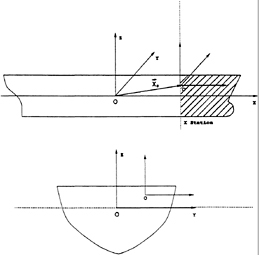
Figure 1: Coordinate System.
2. PROBLEM FORMULATION
Figure 1 illustrates a Cartesian coordinate system ![]() fixed on the mean translating position of the ship which advances in the positive x—direction with a constant velocity U. The positive z—axis points upwards and the origin of the coordinate system is located on the calm water plane. The second coordinate system centered at
fixed on the mean translating position of the ship which advances in the positive x—direction with a constant velocity U. The positive z—axis points upwards and the origin of the coordinate system is located on the calm water plane. The second coordinate system centered at ![]() will be used for the derivation of the wave induced structural loads, carried out in Section 6.
will be used for the derivation of the wave induced structural loads, carried out in Section 6.
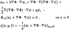
Potential flow is assumed, governed by the velocity potential ![]() which is subject to the Laplace equation in the fluid domain. The nonlinear free surface condition is linearized on the assumption that either the ship hull form is slender or that the ship speed is low. Both these linearization assumptions may be accommodated by the double-body linearization of the free-surface condition, which assumes the decomposition of Ψ into the double-body potential, Φ, the steady wave potential,
which is subject to the Laplace equation in the fluid domain. The nonlinear free surface condition is linearized on the assumption that either the ship hull form is slender or that the ship speed is low. Both these linearization assumptions may be accommodated by the double-body linearization of the free-surface condition, which assumes the decomposition of Ψ into the double-body potential, Φ, the steady wave potential, ![]() , and
, and
the unsteady potential ψ, or
Ψ=Φ+![]() +ψ. (2.1)
+ψ. (2.1)
The flow velocities due to the last two components in (2.1) are assumed small relative to the double-body flow velocity ![]() Φ which far from the ship tends to a uniform flow with velocity (−U,0,0).
Φ which far from the ship tends to a uniform flow with velocity (−U,0,0).
The linearized free surface conditions governing the steady and unsteady wave disturbances have been derived and discussed in Nakos and Sclavounos (1990). They take the form:

(2.2)
for the steady flow, and
(2.3)
for the unsteady flow.
The linearized the ship hull condition takes the familiar form
![]() , on
, on ![]() (2.4)
(2.4)
for the double-body flow,
![]() , on
, on ![]() (2.5)
(2.5)
for the steady flow, and
![]() , on
, on ![]() (2.6)
(2.6)
for the unsteady flow, all applying on the mean position of the ship hull ![]() . In equation (2.6) the summation is carried out over all six rigid-body modes, namely the surge, sway, heave displacements (ξ1,ξ2,ξ3) and the roll, pitch and yaw rotations (ξ4,ξ5,ξ6). The normal vector components nj are defined as
. In equation (2.6) the summation is carried out over all six rigid-body modes, namely the surge, sway, heave displacements (ξ1,ξ2,ξ3) and the roll, pitch and yaw rotations (ξ4,ξ5,ξ6). The normal vector components nj are defined as ![]() follows, and
follows, and ![]() , while the so-called m-terms are defined as in Ogilvie and Tuck (1969) in terms of the double gradients of the double body velocity potential Φ.
, while the so-called m-terms are defined as in Ogilvie and Tuck (1969) in terms of the double gradients of the double body velocity potential Φ.
Frequency Domain Formulation
It is customary in linear seakeeping theory and computation to solve the boundary value problem for the unsteady flow in the frequency domain. Denote by ![]() 0 the velocity potential of a regular surface wave of amplitude A, absolute frequency ω0, heading β, relative to the positive x—axis and wavenumber in deep water,
0 the velocity potential of a regular surface wave of amplitude A, absolute frequency ω0, heading β, relative to the positive x—axis and wavenumber in deep water, ![]() . Relative to the translating coordinate system, it is defined as follows:
. Relative to the translating coordinate system, it is defined as follows:
![]() , (2.7)
, (2.7)
where the complex velocity potential φ0 is given by
(2.8)
with the encounter frequency ω defined as follows
(2.9)
Decomposing the unsteady wave disturbance into incident, diffraction and radiation components and adopting the complex notation (2.7), the unsteady potential may be cast in the form
(2.10)
where φ7 is the complex diffraction potential and φj are the complex radiation potentials due to the harmonic oscillation of the ship in each rigid body mode with unit velocity at the frequency of encounter ω.
3. THE HYDRODYNAMIC FORCES AND EQUATIONS OF MOTION
The linearized unsteady hydrodynamic pressure on the mean position of the ship hull follows from Bernoulli's equation,
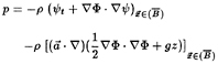
(3.1)
where ![]() denotes the vector oscillatory displacement of the ship surface due to a six-degree-of-freedom oscillatory motion. The second component of (3.1) consists of two terms. The last term contributes the hydrostatic restoring force and moments, while the first term supplies a dynamic correction to the hydrostatic effect which arises from the oscillatory displacement of the ship in the non-uniform steady flow created by the ship forward translation. For the Froude numbers considered in this paper this dynamic contribution to the restoring coefficients was found to be small and was neglected. Yet, at higher Froude numbers this effect may be significant.
denotes the vector oscillatory displacement of the ship surface due to a six-degree-of-freedom oscillatory motion. The second component of (3.1) consists of two terms. The last term contributes the hydrostatic restoring force and moments, while the first term supplies a dynamic correction to the hydrostatic effect which arises from the oscillatory displacement of the ship in the non-uniform steady flow created by the ship forward translation. For the Froude numbers considered in this paper this dynamic contribution to the restoring coefficients was found to be small and was neglected. Yet, at higher Froude numbers this effect may be significant.
The linear equations of motion governing the time-harmonic responses of the ship follow from Newton's law. In complex notation, they accept the familiar form
![]() ,
,
i=1, … 6 , (3.2)
where mij is the ship inertia matrix, ξj the complex amplitude of the ship oscillatory displacement and cij the matrix which which accounts for hydrostatic and inertia restoring effects. The hydrodynamic added-mass and damping coefficients, aij and bij respectively and the exciting forces and moments Xj, are defined as follows
(3.3)
As indicated by (3.1) and (3.3) all hydrodynamic forces are evaluated by direct integration of the hydrodynamic pressure over the mean position of the ship hull. The numerical algorithm implemented in SWAN determines the flow velocity on the panels as part of the solution, therefore, it is unnecessary to apply Stokes' theorem for the evaluation of (3.3) as suggested in Ogilvie and Tuck (1969).
4. THE RANKINE PANEL METHOD
In this section the principal attributes of the Rankine Panel Method developed for the solution of the steady and unsteady free surface problems will be described. Further details may be found in Sclavounos and Nakos (1988) and Nakos and Sclavounos (1990a,b).
Plane quadrilateral panels are distributed over the ship hull and part of the free surface, as illustrated in Figure 3 for the S-175 hull. The potential flow in the fluid domain is solved by an application of Green's second identity for the unknown potentials ![]() ,φ using the Rankine unit source as the Green function. The result is an integro-differential equation for the unknown steady and unsteady potentials and their gradients over the mesh illustrated in the Figure. Four aspects of the Rankine Panel Method implemented in SWAN deserve special mention. They are discussed below:
,φ using the Rankine unit source as the Green function. The result is an integro-differential equation for the unknown steady and unsteady potentials and their gradients over the mesh illustrated in the Figure. Four aspects of the Rankine Panel Method implemented in SWAN deserve special mention. They are discussed below:
1. Bi-Quadratic Spline Scheme—Stability Analysis
A bi-quadratic spline basis function has been introduced for the approximation of the velocity potential over the ship hull and the free surface. The numerical properties of this representation for forward speed free surface flows were studied in Nakos and Sclavounos (1990b). The method was found to be free of numerical damping or amplification, a very desirable property in the computation of ship wave patterns. A stability criterion was developed restricting the selection of the panel aspect ratio relative to the Froude number and frequency rendered non-dimensional by the panel size h. The numerical dispersion of
the method was determined to be of O(h3) which was found to introduce negligible numerical error.
2. Radiation Condition
With Rankine Panel Methods, the proper enforcement of the radiation condition at infinity is essential for their successful use. In SWAN the condition of no waves upstream of the ship has been satisfied by requiring that both the wave elevation and its slope vanish at the upstream boundary of the free surface discretization. The formal derivation of this radiation condition in steady flow is presented in Sclavounos and Nakos (1988), were its preformance for a range of 2D and 3D steady and unsteady flows has been tested and found to be very satisfactory. The transverse and downstream ends of the free surface mesh are successfully treated as free boundaries. For values of the reduced frequency ![]() less than 1/4, a component of the unsteady wave disturbance generated by the ship is known to propagate upstream. In such cases the same upstream radiation condition was found to generate convergent computations of the unsteady flow past the ship for Froude numbers typically larger than 0.15. Seakeeping experiments in the vicinity
less than 1/4, a component of the unsteady wave disturbance generated by the ship is known to propagate upstream. In such cases the same upstream radiation condition was found to generate convergent computations of the unsteady flow past the ship for Froude numbers typically larger than 0.15. Seakeeping experiments in the vicinity ![]() of are unfortunately scarce, therefore the fidelity of the SWAN computations in such cases is to be determined.
of are unfortunately scarce, therefore the fidelity of the SWAN computations in such cases is to be determined.
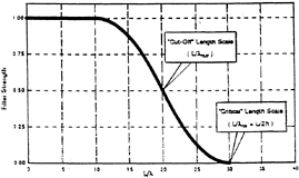
Figure 3: The Low-pass Filter Used for Smoothing the Basis Flow.
3. Filtering Algorithm
The steady and time-harmonic free surface flows past elementary wave singularities have shown that the linearized free surface condition allows for wave disturbances with very small length scales associated with divergent wave systems. The presence of such short scales in ship flows modelled by linearized free surface conditions cannot therefore be ruled out. Moreover, experimental evidence may be misleading when it comes to the existence of short scales in the solution of linearized forward-speed ship flows because of the prevalence in the physical flow of nonlinearity at the bow and viscosity at the stern.
In early computations with SWAN attempts to generate convergent wave pattern predictions in the steady and time-harmonic problems revealed either lack of convergence and the manifestation of short scale spatial oscillations in the numerical solution. Unable to determine the degree to which they are to be attributed to a short scale analytical behaviour in the wave pattern or to numerical error, the decision was taken to filter such short scales out of the numerical solution.
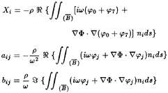
There exist several ways to carry out such a filtering. In the SWAN formulation, as in most double-body linearizations of the free surface condition, short scales are likely to be generated by the sharp gradients of the double-body flow near the ship ends. The low-pass filter shown in Figure 3 is applied to the second-gradients of the double-body flow by discrete convolution in the x—and y—directions. The remaining gradients of Φ which enter in the free-surface conditions (2.2) and (2.3) are not filtered. In Figure 3 two characteristic length scales are defined. The scale λCR denotes the shortest wavelength which can be resolved by the numerical scheme, and equals 2h, where h is the typical grid size in the streamwise direction. In Figure 3 this scale is selected to be 30 times smaller that the ship length. The second length scale λCUT is a parameter of the filter function and denotes the upper bound of the length scales which are to be trusted as accurate in the numerical solution. Numerical experiments suggest that numerical error may be significant for length scales between λCR and λCUT. The former is essentially the Nyquist length scale 2h and is controlled by the selection of the number of panels. The latter is a parameter of the filter which may be selected independently of the number of panels.
In the SWAN computations reported in the present paper λCUT was selected equal to L/15, where L is the ship length. The SWAN computations of the wave pattern have been found to be convergent for such a cutoff lengthscale, therefore the numerical solution of the linear boundary-value problem should be trusted for wavelengths larger than λCUT. Such a claim cannot be made for shorter scales, regardless of their analytical or physical relevance. Further properties of this filtering algorithm in the computation of Kelvin wave patterns and wave resistance are discussed in Nakos and Sclavounos (1993).
4. Iterative Solution of Linear System
The efficient solution of the real or complex linear system obtained from RPM formulations is essential for the utility of such methods in practice. The associated matrices are full, asymmetric and generally poorly conditioned, therefore robust and efficient solution algorithms must be available for their solution.
The linear systems in SWAN are presently solved by block Gauss-Siedel iteration, equipped with a minimum-residual acceleration scheme. The block size is typically selected to be a quarter of the matrix size, leading to convergence in about 20–30 iterations for the unsteady problem. This rate of convergence is found to be insensitive to the number of panels used as long as the block/matrix ratio is kept equal to 1/4.
A preconditioner is currently under development for the SWAN sub-matrix which is associated with the free surface grid. Preliminary results indicate that the rate of convergence of basic iterative methods on the preconditioned matrix are increased and the need for block iteration is eliminated. The objective is the development of a rapidly convergent preconditioned iterative method based on the efficient access and computation of large matrix-vector products.
5. THE FREE SURFACE WAKE
As outlined in the Introduction, for ships with transom or flared sterns, the proper treatment of the local free surface flow physics calls for the introduction of a free surface wake, consisting of a strip of panels trailing the ship as illustrated in Figure 2. Denoting by h(x,y) the vertical offset of the ship hull near the stern and by ζ(x, y) the free surface elevation just downstream of it as defined by equation (2.2), the following smooth detachment conditions are enforced at the stern in the case of steady flow:
ζ(xT,y)=h(xT,y) (5.1)
(5.2)
These conditions state that the free surface elevation at the upstream end of the free surface wake leaves the stern smoothly, preserving the continuity of the steady flow streamlines.
The same conditions are enforced in the time-harmonic problem with the unsteady free surface elevation now defined by expression (2.3). In both steady and unsteady problems the smooth detachment conditions (5.1) and (5.2) merely enforce a finite velocity over the portion of the stern which sheds a wake. The analogy with the linearized Kutta conditions in lifting surface theory is evident.
Expressions (5.1)–(5.2) are expected to properly model stern flows past transom sterns of small or zero draft. In either case the two conditions are transferred on the z=0 plane and enforced on the upstream side of the wake. In the numerical implementation of (5.1) and (5.2) it was found that the most essential condition to enforce is the continuity of the velocity potential. This finding is consistent with similar implementations of the linearized Kutta condition, also known as Morino condition, in potential based steady and unsteady lifting flows.
6.
STRUCTURAL LOADS
Figure 1 illustrates two Cartesian coordinate systems, fixed relative to the ship hull and translating with its forward speed. The reference coordinate system (x,y,z) has been defined above in connection with the formulation of the free surface boundary value problems. The second coordinate system, is obtained by parallel shift of the axes of the reference frame by the vector  0. It is centered at an arbitrary point O with
respect to which all components of the structural loads exerted by inertia and fluid forces on the shaded portion of the ship hull will be determined.
All forces will be linearized about the mean position of the ship hull, therefore use will be made of the linear version of the skew symmetric rotation matrix T,
(6.1)
where (ξ4,ξ5,ξ6) are the linear roll, pitch and yaw ship displacements. It follows that the linear displacement of a point on or inside the ship hull, fixed relative to the reference frame (x,y,z), is defined by
(6.2)
where ![]() denotes the vector of linear ship displacements and the vector
denotes the vector of linear ship displacements and the vector ![]() is to be regarded as a quantity independent of time.
is to be regarded as a quantity independent of time.
The fluid pressure acting on the wetted part of the shaded portion of the ship hull is determined from the solution of the steady and time harmonic free surface flows described above. The resultant forces and moments follow by direct integration over the ship hull of the hydrodynamic pressure as defined by (3.1). For the Froude numbers considered in the present study, the contribution to the structural loads by the steady pressure was found to be small and was ignored.
Denoting by S the mean wetted surface of the shaded portion of the ship hull, by C the mean position of its waterline and V the volume over which mass elements are distributed, the unsteady force vector acting over (S,V) by fluid and inertia forces follows in the form

(6.3)
where p is the unsteady pressure, ηs is the steady and ηr the relative wave elevations along the ship waterline, the latter defined as the difference between the total unsteady wave elevation and the vertical ship displacement. The corresponding moment vector acting over the same portion of the ship hull, about the axes of the coordinate system centered at the point O, is defined as follows

(6.4)
In (6.3) and (6.4), the second terms arise from the fluid pressure forces which include the hydrostatic contribution by virtue of the last term in the definition (3.1) of the pressure. The leading terms account for the inertia effect contributed by the acceleration of the differential mass dm and the last terms represent the restoring force and moment, respectively, contributed by the mass of the shaded part of the ship as it undergoes rotational oscillations. A more detailed derivation of (6.3) and (6.4) is carried out by Helmers (1992)(private communication).
The waterline integrals may be seen to depend on the steady wave elevation along the waterline which is assumed to be large for flared geometries. For the vertical loads, the normal vector component n3 may be seen to be equal to the sine of the the flare angle which vanishes for wall sided ships. The magnitude of the waterline integral contribution to the vertical wave loads will be studied in Section 8. Expressions (6.3) and (6.4) represent the unsteady contribution to the structural loads which must be added to the static loads acting upon a ship in calm water.
By virtue of the three dimensional nature of the hydrodynamic solution determined by SWAN, the force and moment vectors defined by (6.3) and (6.4) may be evaluated at any arbitrary point O over the ship surface or its interior, as the structural analysis may require. The evaluation of the volume integrals accounting for the
dynamic and restoring inertial effects may be easily evaluated by a summation over as many mass points as are necessary to distribute over the ship interior in order to represent its inertia properties. This is the method adopted in SWAN.
7. NUMERICAL RESULTS
7.1 Kelvin Wave Patterns Past Transom Stern Ships
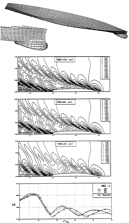
Figure 4 illustrates the hull discretization of the transom stern DTMB model 5415 consisting of 80 panels along the ship length and 10 panels along its half section. A strip of panels trailing its transom is added with the smooth detachment conditions (5.1) and (5.2) enforced at its upstream end. Computations of the Kelvin pattern at a Froude number 0.25 are presented, where their convergence is studied as a function of the number of panels along the ship length. A comparison is also carried out of the computed Kelvin wake spectrum with the measurements carried out in the ‘wakeoff' comparative study of Lindenmuth, Ratcliffe, and Reed (1991) with good agreement. In all computations the panel aspect ratio α was taken equal to 1 on the free surface and near the ship hull. This selection of the aspect ratio typically requires a large number of panels on the free surface but has been found to lead to convergent computations.
7.2 Hydrodynamic Forces and Motions of the SL7 and S-175 Hulls
Computations have been carried out of the heave and pitch damping coefficients of the SL7 and S-175 hulls. Both hulls have flared geometries at the stern which must be taken into account properly for the accurate computation of their seakeeping properties.
The steady problem is solved first about the calm water position of the hull and its sinkage, trim and steady wave profile are evaluated along the waterline and downstream of the stern. Based on this information, the new position of the ship waterline relative to the ship hull is determined and the extent of the ship stern that gets wet is determined by intersecting the steady wave profile with the stern profile, including effects of sinkage and trim. The SL7 stern possesses a long countertop, a significant portion of which gets wet as a result of the sinkage, trim and steady elevation downstream of the stern. A similar but less pronounced effect may be observed for the S-175 hull and generally for hull shapes with significant flare at their stern. The corresponding effect at the bow is less pronounced for nearly vertical bow stems.
Computations of the hydrostatic, impedance forces and ship motions for the linear and ‘nonlinear' wetted surface of the ship hull revealed a strong sensitivity of the motions on the steady wave profile effect on the hydrostatic coefficients. The hydrodynamic coefficients were found not to be appreciably different in the two cases and they have thus been computed about the linear wetted surface, for the sake of simplicity.
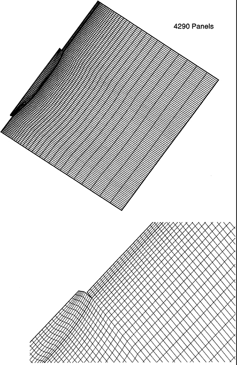
The proper discretization of the free surface in the vicinity of the stern of a flared hull is essential for the robustness and convergence of the numerical solution. An attempt to distribute panels around flared sterns without the introduction of a wake revealed a strong sensitivity of the numerical solution on the number and arrangement of panels. The introduction of a wake strip of panels trailing the stern was found to cure this problem and lead to convergent computations. The panel arrangement in the vicinity of the stern of the S-175 is illustrated in Figure 2 where the shallow portion of the stern has been removed and an equivalent transom was introduced as indicated in the Figure.
Convergence tests were carried out using the grid arrangement shown in Figure 2. The parameters varied included the panel aspect ratio and the total number of panels. For both ship hulls and for all frequencies and Froude numbers tested, convergence to within graphical accuracy was achieved, using up to about 5,000 panels on half the ship hull, free surface and wake with the panel aspect ratio varying from 1.5 to 2.0, defined at the ratio of the stream wise to the transverse dimensions of a typical panel in the vicinity of the ship waterline. The aspect ratio of 1.5 was selected in the final computations. The extent of the free surface grid relative to the ship dimension is illustrated in Figure 2.
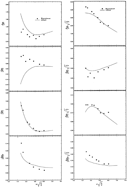
The heave and pitch added mass and damping coefficients of the SL7 hull advancing at a Froude
number 0.3 are illustrated in Figure 5. The computations by SWAN are compared to the experimental measurements by O'Dea and Jones (1983). The corresponding computations for the S-175 advancing at a Froude number 0.275 are plotted in Figure 7. Computations by SWAN of the heave and pitch exciting forces for the SL7 advancing in head waves are compared to experiments in Figure 6. The agreement is very satisfactory, as is usually the case with the exciting forces.
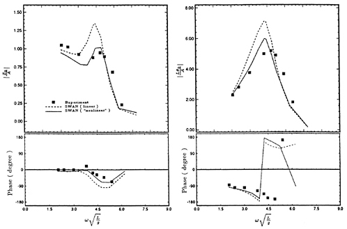
Heave and pitch motion amplitude and phase computations by SWAN for the SL7 are compared to experiments in Figure 8 in head waves and a Froude number Fr=0.3. The SWAN predictions marked as ‘nonlinear' have accounted for the effect of the hull sinkage, trim and steady wave profile upon the restoring coefficients. The corresponding head wave heave and pitch motion computations for the S-175 hull at a Froude number 0.275, are illustrated in Figure 10. The experimental measurements for the S-175 hull have been reported by the ITTC and are discussed in more detail by Dalzell (1992).
A clear trend emerges from these computations. The account of the nonlinear effect described above reduces the amplitude of the heave and pitch motions at resonance by an appreciable amount, leading to a good agreement with experimental measurements. Both the linear SWAN computations and strip theory tend to overpredict the heave and pitch motions at resonance, a trend which is not evident for wall sided geometries like the Wigley and the Series 60 hull, studied in Nakos and Sclavounos (1990).
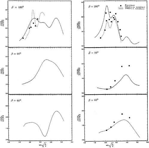
Heave and pitch motions of the S-175 advancing at Fr=0.275 in beam (β=90 deg) and quartering (β=60 deg) waves are plotted in Figure 10 and compared with good agreement to the experimental measurements reported by the ITTC. All hydrodynamic force and motion computations reported in this study correspond to Froude number and frequency combinations such that the values of the reduced frequency ![]() =ωU/g are greater than 1/4.
=ωU/g are greater than 1/4.
7.3 Heave and Pitch Motions of an IACC Yacht Hull
Figure 11 illustrates the body plan and free surface discretization of an International America's Cup Class generic yacht hull, code named PACT (Partnership for America's Cup Technology) baseline geometry, characterized by its small draft and significant flare along its entire length. The robust solution of the steady and unsteady flows around such hulls necessitates the introduction of a free surface wake which may be seen trailing the yacht stern in Figure 11. The wake panels are distributed around the flared portion of the stern, since in this case the definition of an equivalent transom is not as evident as for the SL7 and S-175 hulls.
Computations of the heave and pitch motion amplitudes including the nonlinear steady state effect discussed above are compared in Figure 11 with experimental measurements by Cohen and Beck (1992). Consistently with the SL7 and S-175 computations, the heave and pitch motion amplitudes are found not to display a resonant peak, which is clearly visible in the linear SWAN computations not shown in the figure. Further seakeeping and added resistance computations for the PACT and other yacht hull geometries are presented in Sclavounos and Nakos (1993).
8. WAVE INDUCED STRUCTRURAL LOADS ON THE SL-7 and S-175 HULLS
Computations were carried out of the vertical shear force and bending moment induced at the midship section and about a transverse axis coinciding with the z=0 plane. Expressions (6.3) and (6.4) were used with all integrations carried out over the fore half of the ship hull. The wave induced loads have been determined using both the linear and nonlinear heave and pitch motion amplitudes evaluated in the manner described in Section 7. Furthermore the contribution to the loads from the waterline integrals in (6.3) and (6.4) which account for the effect of flare has been isolated and compared to the surface and volume integrals in the same expressions.
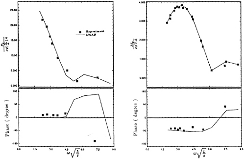
The vertical shear force and bending moment induced by head waves on the SL7 hull are presented in Figure 9. SWAN computations using the linear and nonlinear heave and pitch motion amplitude predictions are shown and the latter are found to be in very good agreement
with the measured values. It is noteworthy that the account of the nonlinear effect in the motion amplitude tends to decrease the peak value of the shear force modulus and increase the corresponding modulus of the bending moment, consistently with the experimental trend.
The corresponding head wave shear force and bending moment computations for the S-175 hull are presented in Figure 12. Again the wave load predictions based on the ‘nonlinear' heave and pitch motions are in better agreement with the experimental measurements and as for the S-175 hull are found to differ appreciably from their linear counterparts. The SWAN wave load predictions in beam and quartering waves are also illustrated in Figure 11 using the ‘nonlinear' heave and pitch motions amplitudes. The agreement with experiments, where available, is again seen to be satisfactory.
The importance of the waterline contribution to the wave loads is demonstrated in Figure 12 where the S-175 head wave midship bending moment defined by expression (6.4) is plotted with and without the waterline terms. It is evident that ignoring the waterline integral, may lead to a marked underprediction of the bending moment. This trend is also evident in the shear force predictions and for other wave headings. Recalling that the waterline-integral contributions are absent for wall-sided hull geometries, it is concluded that the effect of flare near the fore end of a ship hull is responsible for a siginificant component of the vertical wave induced loads, as intuition alone might suggest.
9. SUMMARY
Seakeeping and wave induced structural load computations have been presented for the SL7, S-175 hulls and an IACC yacht with the Rankine Panel Method SWAN. All three hulls are characterized by the presence of significant flare near their bow and stern regions. Extensions of SWAN are developed which account for the effects of flare, driven by the flow physics and aiming to generate robust and accurate numerical predictions for the ship motions and wave loads. They include; a) the introduction of a wake of panels trailing transom and flared sterns, equipped with Kutta type conditions of finite velocity, b) the account of the effect of the ship sinkage, trim and steady wave profile interaction with the stern upon the hydrostatic coefficients and c) the derivation of waterline corrections to the linearized wave load definitions, which account for effects of flare.
Heave and pitch motion computations, corrected for the effects of flare as outlined above, are found to be in very good agreement with experiments, particularly near resonance where flare effects appear to introduce a detuning to the heave/pitch oscillation and a reduction of their respective amplitudes. Computations of the vertical shear force and bending moments in head and oblique waves for the SL7 and the S-175 hulls show a strong dependence upon, a) the use of the ‘nonlinear' heave and pitch motion amplitudes, corrected for the effects of flare at the stern, and b) the account of waterline terms in the definition of the loads, which arise only when flare is present near the ship bow.
10. Acknowledgements
This study has been supported by the Office of Naval Research (Contract N00014–91-J-1509), David Taylor Model Basin (ONR Contract N00014–92-J- 1776) and A.S., Veritas Research. The study of the seakeeping properties of the IACC yacht hull has been supported by PACT (Partnership for America's Cup Technology).
References
Cao, Y., Schultz, W.W. and Beck, R.F. 1992, “Three Dimensional Unsteady Computations of Nonlinear Waves Caused by Underwater Disturbances”. Proceedings 18th Symposium on Naval Hydrodynamics, Ann Arbor, Michigan .
Dalzell, J.F., Thomas, W.L., III and Lee, W.T., 1992, “Correlations of Model Data with Analytical Load Predictions for Three High Speed Ships”, Report SHD-1374–02, Naval Surface Warfare Center.
Dawson, C.W., 1977, “A practical computer method for solving ship-wave problem”, 2nd International Conference on Numerical Ship Hydrodynamics, USA .
Gadd, G.E., 1976, “A method for computing the flow and surface wave pattern around full forms”, Trans. Roy. Asst. Nav. Archit., Vol 113, pg. 207.
Jensen, G., and Soding, H., 1989, “Ship Wave Resistance Computations”, Finite Approximations in Fluid Mechanics II, Vol 25.
Kim, Y.H., and Lucas, T., 1990, “Nonlinear Ship Waves”, Proceedings of the 18th Symposium on Naval Hydrodynamics, Ann Arbor, MI, USA.
Lindenmuth, W.T., ratcliffe, T.J. and Reed, A. M., 1991, “Comparative Accuracy of Numerical Kelvin Code Predictions—Wake-Off”. DTMB Report 91/004, Bethesda, Maryland.
Maskew, B., 1992, “Prediction of Nonlinear Wave/Hull Interactions on Complex Vessels ”, Proceedings of the 19th Symposium on Naval Hydrodynamics, Seoul, Korea.
Nakos, D.E. and Sclavounos P.D., 1990b, “On steady and unsteady ship wave patterns”, Journal of Fluid Mechanics, Vol. 215, pp. 256–288.
Nakos, D.E. and Sclavounos P.D., 1990a, “Ship Motions by a Three Dimensional Ranking Panel Method”, Proceedings of the 18th Symposium on Naval Hydrodynamics, Ann Arbor, MI, USA.
Nakos, D.E. and Sclavounos, P.D. 1993, “Kelvin Wakes and Wave Resistance of Cruiser and Transom Stern Ships ”. To appear in Journal of Ship Research.
Nakos, D.E., Kring, D.C. and Sclavounos, P.D., 1993, “Ranking Panel Methods for Time-Domain Free Surface Flows” 5th International Conference on Numerical Ship Hydrodynamics, USA .
O'Dea, J.F. and Jones, H.D., 1983, “Absolute and Relative Motion Measurements on a Model of a High-speed Containership”, Proceedings of the 20th American Towing Tank Conference, Hobeken, NJ, USA, Vol. II.
Raven, H., 1992, “A Practical Nonlinear Method for Calculating Ship Wavemaking and Wave Resistance”, Proceedings of the 19th Symposium on Naval Hydrodynamics, Seoul, Korea.
Reed, A.M., Telste, J.G., Scragg, C.A. and Liepmann, D., 1990, “Analysis of Transom Stern Flows”, Proceedings of the 18th Symposium on Naval Hydrodynamics, Ann Arbor, MI, USA.
Rosen, B.S., Laiosa, J.P., Davis, W.H. and Stavetski, D., 1993, “SPLASH Free-Surface Flow Code Methodology for Hydrodynamic Design and Analysis of IACC Yachts”. Proceedings of 11th Chesapeake Sailing Yacht Symposium, Annapolis, Marland.
Sclavounos, P.D. and Nakos, D.E., 1988, “Stability Analysis of Panel Methods for Free-Surface Flows with Forward Speed”, Proceedings of the 17th Symposium on Naval Hydrodynamics, The Hague, The Netherlands.
Sclavounos, P.D. and Nakos, D.E., 1993, “See-keeping and Added Resistance of IACC Yachts by a Three Dimensional Panel Method”, 11th Chesapeake Sailing Yacht Symposium, Annapolis, IN, USA.
Xia, F., 1986, “Numerical Calculations of Ship Flows with Special Emphasis on the Free Surface Potential Flow”, Doctoral Thesis, Chalmers University of Technology, Sweden.


DISCUSSION
by Professor Robert Beck, University of Michigan, Ann Arbor
Do you have an explanation to the hump that appears in the bending moment curve at high frequencies?
Author's Reply
I would attribute the mid-ship bending moment hump at high frequencies to constructive/destructive interference effects caused for wavelengths shorter than the ship length of nature similar to that encountered in the high-frequency behavior of the heave and pitch exciting forces. The amplitude of these effects is magnified in the mid-ship bending moment and shear force integrations which are carried out over half the ship surface. Similar interference effects in the exciting force evaluation are less pronounced due to cancellation in the respective integration which is carried out along the entire ship length.
DISCUSSION
by Emilio Campana, INSEAN, Italian Ship Model Basin
In your paper you say that for the solution of the large linear system a wave preconditioner, based on the free surface grid, has been used. Can you give some more details?
Author's Reply
We have developed a reconditioner which is custom designed for real and complex matrix equations arising in Rankine panel methods. The preconditioner is based on the approximate inversion of the sub-matrix associated with the free-surface mesh by a discrete FFT technique. The resulting preconditioned matrix (real for the steady and complex for the unsteady problem) becomes diagonally dominant and its inversion becomes possible by point, as opposed to block, minimum residual accelerated Jacobi and Gauss-Siedel iteration. The rate of convergence of this new iterative scheme was found to be uniformly faster than the original block iteration method over a broad range of frequencies and speeds.
Calculation of Transom Stern Flows
J.G.Telste and A.M.Reed
(David Taylor Model Basin, USA)
ABSTRACT
This paper presents a method of calculating the flow near a transom stern ship moving forward at a moderate to high steady speed into otherwise undisturbed water. The speed is assumed to be sufficient to guarantee smooth flow separation at the stern and a dry transom. In addition, conditions necessary to justify the assumption of potential flow are assumed. Modified free-stream linearization is used to obtain a Neumann-Kelvin boundary value problem in which the usual linearization about the mean free-surface level is replaced in the area behind the transom stern by linearization about a surface originating at the hull-transom intersection. A Rankine singularity integral equation is presented for obtaining the solution of the resulting mathematical boundary-value problem. The integral equation involves line integrals around the hull and has been designed so that it greatly reduces the requirement of using forward finite differences to enforce the radiation boundary condition. The approach permits the presence of free-surface dipoles and provides a mechanism for carrying lift downstream from a transom stern in accordance with the work of various researchers who, in recent years, had suggested that lift effects are an important component of wave resistance under certain conditions. Computational results are presented for two transomstern ships.
NOMENCLATURE
|
CWP |
wave resistance coefficient computed from wave spectral energy (=2 RW/ϱSU2) |
|
E(x,y) |
surface behind a transom stern on which linearized free-surface boundary conditions are applied (=SE) |
|
F |
Froude number |
|
|
sine component of the free-wave spectrum |
|
g |
gravitational acceleration |
|
|
cosine component of the free-wave spectrum |
|
k0 |
fundamental wave number (=g/U2) |
|
L |
ship length |
|
|
unit normal directed into the fluid |
|
(nx,ny,nz) |
components of the normal vector |
|
r |
distance from the singular point |
|
Rw |
wave resistance |
|
S |
wetted surface area of the hull |
|
SB |
hull surface (zero sinkage and trim) |
|
SE |
surface behind a transom stern on which linearized free-surface boundary conditions are applied (=E(x,y)) |
|
|
projection of SE onto the mean free-surface level |
|
SF |
mean free-surface level |
|
U |
ship speed |
|
u |
transverse wave number (=secθ tanθ) |
|
ν |
longitudinal wave number (=secθ) |
|
|
vector notation of the field point (x,y,z) |
|
(x,y,z) |
coordinates of the field point |
|
|
point on the hull-transom intersection |
|
Z(x,y) |
wave elevation |
|
|
vector notation for a singular point (ξ,η,ζ) |
|
(ξ, η, ζ) |
coordinates of the singular point |
|
|
density of water |
|
Φ |
velocity potential |
|
|
perturbation potential |
|
θ |
angle from which the transverse wave number is computed |
INTRODUCTION
Before the appearance of high-speed computers, ship designers had to rely solely on systematicseries experiments for designing criteria. With the great improvement in the capability of computing quantities such as wave resistance, trim moment, and the Kelvin wave pattern that has occurred especially since the 1970's, designers now frequently rely on a complementary combination of experiments and computer simulations. The increased computational capability has come about because of the effort that has been expended through the years in the development of computer codes to simulate flow near ships moving steadily into otherwise undisturbed water— the wave resistance problem. Computational results for several of these codes can be seen in the “Wake-Off” report of Lindenmuth et al. (1). One of the conclusions of that report was that the predictions of Kelvin wave pattern for ships with transom, sterns were poor.
Since the “Wake-Off,” additional effort has been expended in trying to properly model flow in the neighborhood of the transom stern of a translating ship. Results of such work are presented in the papers of Cheng (2), Reed et al. (3), and Nakos and Sclavounos (4). In their paper, Nakos and Sclavounos present computational results in which a lifting surface originating at the stern is present. Kutta-like conditions are enforced at the stern. For shallow transom sterns the wake is collapsed onto the mean free-surface level. Reed et al. present various arguments to show that it is reasonable and even necessary to include a lift model for flows in the vicinity of a moderate to high-speed transom stern ship, as is done to model the flow about three-dimensional wings. The arguments were based on analogies with high-speed planing craft and ventilated hydrofoils at moderate speeds, as well as the theoretical work and analysis of experimental work of Tulin and Hsu (5). The point of the argumentation was that under certain conditions effects due to lift form a significant component of the wave resistance. Reed et al. present the effects of including a lift model in Rankine and Havelock singularity codes. The effects of lift could be more easily separated in the computational results from the Havelock singularity code, where it was shown that lift modifies the diverging waves of the Kelvin wave pattern originating at the stern. Additionally, it was shown that the strength of the dipole distribution along the transom has a shape similar to that of an elliptic loading on a three-dimensional lifting surface. The effect of lift in the Rankine singularity code could not be distinguished so easily.
This paper presents a method of calculating the flow near a transom stern ship moving forward at a moderate to high steady speed into otherwise undisturbed water. This is a Rankine singularity method in which several enhancements have been made so that the effect of including lift can be seen more clearly in the computational results. The speed is assumed to be sufficiently high to guarantee smooth flow separation at the stern and a dry transom. In addition, conditions necessary to justify the assumption of potential flow are assumed. A modified free-stream linearization is used to obtain a Neumann-Kelvin boundary value problem. In this linearization scheme, for most of the free surface, the usual linearization is used. However, behind the transom, the usual linearization about the mean free-surface level is replaced by linearization about a surface originating at the hull-transom intersection. A Rankine singularity integral equation is presented for obtaining the solution of the resulting mathematical boundary value problem. The integral equation involves line integrals around the hull and has been designed so that it greatly reduces the requirement of using forward finite differences to enforce the radiation boundary condition. The approach permits the presence of free-surface dipoles and provides a mechanism for carrying lift downstream from a transom stern.
MATHEMATICAL FORMULATION
A coordinate system is fixed to the ship with the origin inside the hull on the mean free-surface level so that x is positive downstream, z is positive above the mean free-surface level, and y is positive on the starboard side. In this coordinate system a uniform stream of speed U is flowing past the hull in the positive x-direction.
Boundary Value Problem
Conditions necessary for potential flow are assumed. For now, a cruiser stern is assumed and freestream linearization about the mean free-surface level is used. The total potential Φ is written as the sum of the free-stream potential Ux and a disturbance potential ![]() :
:
Φ=Ux+![]() (1)
(1)
Then the following dimensional equations characterize the boundary value problem:
∇2Φ=∇2![]() =0 (2)
=0 (2)
UZX−![]() z=0 on SF (3)
z=0 on SF (3)
U![]() x+gZ=0 on SF (4)
x+gZ=0 on SF (4)
(5)
where SF is the mean free-surface level, SB is the hull surface below the mean free-surface level, Z is the free-surface height, and ![]() is the unit normal directed into the fluid. Eqs. (3) and (4) are the kinematic and dynamic free-surface boundary conditions, which are to be satisfied on the mean free-surface level. To ensure a unique solution, a radiation condition that no waves propagate upstream of the hull must also be satisfied.
is the unit normal directed into the fluid. Eqs. (3) and (4) are the kinematic and dynamic free-surface boundary conditions, which are to be satisfied on the mean free-surface level. To ensure a unique solution, a radiation condition that no waves propagate upstream of the hull must also be satisfied.
After normalizing lengths by the length L of the ship and velocities by the speed U, the equations take the form
Φ=x+![]() (6)
(6)
![]() 2Φ=
2Φ=![]() 2
2![]() =0 (7)
=0 (7)
Zx−![]() z=0 on SF (8)
z=0 on SF (8)
![]() +Z/F2 =0 on SF (9)
+Z/F2 =0 on SF (9)
(10)
where F is the Froude number given by ![]() . The nondimensional kinematic and dynamic boundary conditions, eqs. (8) and (9), can be combined into the single boundary condition
. The nondimensional kinematic and dynamic boundary conditions, eqs. (8) and (9), can be combined into the single boundary condition
F2![]() xx+
xx+![]() z=0 (11)
z=0 (11)
which is to be applied on the mean free-surface level.
Integral Equation
Green's second identity can be used to obtain an integral equation for the solution of eqs. (7)–(10). If the integral over a hemispherical surface beneath the mean free-surface level vanishes as that surface is expanded to infinity, then the integral equation

(12)
holds for ![]() . All integrals other than the first or third one are regular. If
. All integrals other than the first or third one are regular. If ![]() , then the first integral is a principal-value integral; otherwise
, then the first integral is a principal-value integral; otherwise ![]() and the third integral is a principal-value integral. Eq. (11), the combined free-surface boundary condition, was used to obtain the last term in its present form.
and the third integral is a principal-value integral. Eq. (11), the combined free-surface boundary condition, was used to obtain the last term in its present form.
It is intended to solve the boundary value problem with a low-order Rankine singularity panel code in which the source and dipole distributions over each panel are uniform. Such codes often use finite differences to approximate the derivative of the potential in the last term of the integral equation. However, as is stated in the recent paper by Lechter (6), there is really no satisfactory finite difference scheme for Rankine singularity methods. The situation is worsened by the appearance of the second derivative ![]() rather than a first derivative. In this case, however, the need for finite differencing can be greatly reduced by applying Stokes ' theorem to the last term of eq. (12). Then a collocation point shifting scheme together with analytic differentiation can be used over most of the free surface. This scheme is similar to the scheme used by Jensen (7). As is pointed out in (6), there are difficulties associated with Jensen's method, especially at low speeds; even so, at the moderate to high speed flows with which this paper deals, the method is an improvement over one in which
rather than a first derivative. In this case, however, the need for finite differencing can be greatly reduced by applying Stokes ' theorem to the last term of eq. (12). Then a collocation point shifting scheme together with analytic differentiation can be used over most of the free surface. This scheme is similar to the scheme used by Jensen (7). As is pointed out in (6), there are difficulties associated with Jensen's method, especially at low speeds; even so, at the moderate to high speed flows with which this paper deals, the method is an improvement over one in which ![]() is approximated by forward finite differences. The first application of Stokes' theorem follows a simple use of the chain rule for differentiation. The result is
is approximated by forward finite differences. The first application of Stokes' theorem follows a simple use of the chain rule for differentiation. The result is
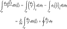
(13)
in which the line integral is counterclockwise around the outer edges of the computational region and clockwise around the hull. The x-derivative in front of the surface integral was obtained from the symmetry of r with respect to ![]() and
and ![]() and from the fact that the integration variable is independent of x. The range of integration for the surface integrals is taken to be the finite portion of the mean free-surface level which is to be paneled later. If the computational domain has sides parallel to the x-z plane, then the line integral has nonvanishing contributions only from around the hull, along the upstream boundary, and along the downstream boundary. The technique can be used again to remove the remaining derivative from inside the surface integral. The result is
and from the fact that the integration variable is independent of x. The range of integration for the surface integrals is taken to be the finite portion of the mean free-surface level which is to be paneled later. If the computational domain has sides parallel to the x-z plane, then the line integral has nonvanishing contributions only from around the hull, along the upstream boundary, and along the downstream boundary. The technique can be used again to remove the remaining derivative from inside the surface integral. The result is

Fig. 1—Top view of surfaces defined for a transom-stern ship.
(14)
Therefore, the final form of the integral equation is
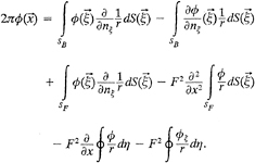
(15)
Transom Stern
Flow past a ship with a transom stern is now considered. The flow is assumed to separate smoothly at the hull-transom intersection. As before SB denotes the hull surface beneath the mean free-surface level. In this case, however, SF denotes the mean free-surface level only for that portion which is not directly behind the stern. There is an additional surface SE which extends from the separation line at the hull-transom intersection to downstream infinity. Eventually, it would be desirable for SE to vary with respect to distance downstream from the hull so that the surface approaches the mean free-surface level downstream of the stern. In this paper, however, SE does not vary in x and so forms a cylindrical surface downstream of the transom stern. It is assumed that ![]() is a smooth surface. The surfaces, viewed from above, are depicted in Fig. 1.
is a smooth surface. The surfaces, viewed from above, are depicted in Fig. 1.
Under the same conditions that were required in the case of a cruiser stern, Green's second identity can be used to obtain the integral equation
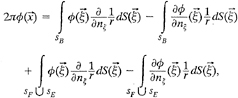
(16)
which is valid for ![]() . For
. For ![]() , the first integral is a principal-value integral; for
, the first integral is a principal-value integral; for ![]() , the third integral is a principal-value integral; otherwise, the integrals are regular. To continue as before, the normal derivative in the last integral must be expressed in terms of the potential and its tangential derivatives on the boundary. If the surface
, the third integral is a principal-value integral; otherwise, the integrals are regular. To continue as before, the normal derivative in the last integral must be expressed in terms of the potential and its tangential derivatives on the boundary. If the surface ![]() is given by the equation
is given by the equation
z−E(x,y)≡0, (17)
then the unit normal directed into the fluid is given by
(18)
and the last term of the integral equation can be rewritten as
 . (19)
Here S′E refers to the projection of SE onto the mean free-surface level.
On the actual free surface z=Z(x, y), which is to be distinguished from the surface z=E(x, y), the nonlinear kinematic and dynamic free-surface boundary conditions are given by

(20)
and
(21)
respectively. It is assumed that ![]() , although it might be argued that
, although it might be argued that ![]() y is not negligible in the vicinity of deep transoms with steep side walls.
y is not negligible in the vicinity of deep transoms with steep side walls.
After discarding these terms, the dynamic free-surface boundary condition becomes
![]() x+Z/F2=0 on z=Z(x,y). (22)
x+Z/F2=0 on z=Z(x,y). (22)
Expanding the factors involving the potential in eqs. (20) and (22) in Taylor series about z=E(x,y) and dropping all terms of the series expansions except the lowest order terms, we obtain

(23)
and
(24)
on z=E(x, y). Eq. (24) can be differentiated with respect to x and combined with eq. (23) to obtain

(25)
on z=E(x,y) which, if we assume ![]() , becomes
, becomes

(26)
on z=E(x,y). This equation is used to eliminate ![]() ζ from the the right hand side of eq. (19):
ζ from the the right hand side of eq. (19):
(27)
If ![]() , then eq. (27) becomes
, then eq. (27) becomes
![]() (28)
(28)
and eq. (16) becomes
 (29)
(29)
which is almost the same as eq. (12). The application of Stokes' theorem proceeds as it does for the case of a cruiser stern and we obtain the integral equation
(30)
This equation is the final form of the integral equation for the case of a transom stern hull.
Free-Wave Spectrum and Wave-Pattern Resistance
We wish to compute the magnitude of the free-wave spectrum whose sine and cosine components ![]() (u) and
(u) and ![]() (u) are defined in eq. (35) of Eggers et al. (8). The definitions assume that all lengths have been normalized by the inverse of the fundamental wave number k0. The same normalization applies to
(u) are defined in eq. (35) of Eggers et al. (8). The definitions assume that all lengths have been normalized by the inverse of the fundamental wave number k0. The same normalization applies to ![]() ,
, ![]() , and the magnitude of the spectrum. The transverse wave number u has been normalized by k0.
, and the magnitude of the spectrum. The transverse wave number u has been normalized by k0.
The free-wave spectrum is calculated from a pair of transverse wave cuts by a method derived by Sharma (9). Sharma, in contrast to Eggers et at., retained dimensions. Taking into account this difference, ![]() and
and ![]() are reproduced here in terms of the nondimensional variables of this paper. If the two transverse wave cuts are Z1(y)=Z(x1,y) and Z2(y)≡Z(x2,y), then
are reproduced here in terms of the nondimensional variables of this paper. If the two transverse wave cuts are Z1(y)=Z(x1,y) and Z2(y)≡Z(x2,y), then
(31)
and
(32)
where
(33)
(34)
and
(35)
for k=1,2.
Using eq. (2.49) of Sharma, the wave resistance RW can be written in terms of ![]() and
and ![]() . The corresponding nondimensional wave-pattern resistance CWP is given by
. The corresponding nondimensional wave-pattern resistance CWP is given by
(36)
where S is the wetted area and L is the length of the hull.
NUMERICAL IMPLEMENTATION
The hull surface and the finite portion of ![]() within the finite computational domain are approximated by strips of flat rectangular panels. Strips on SE originate at the hull-transom intersection; strips on SF originate at the computational boundary upstream of the hull. For the time being, the upstream panel in each strip of SF is assumed to have approximately twice the longitudinal dimension of those panels immediately downstream from it.
within the finite computational domain are approximated by strips of flat rectangular panels. Strips on SE originate at the hull-transom intersection; strips on SF originate at the computational boundary upstream of the hull. For the time being, the upstream panel in each strip of SF is assumed to have approximately twice the longitudinal dimension of those panels immediately downstream from it.
On each panel, the perturbation potential ![]() and its derivative ∂
and its derivative ∂![]() /∂nξ in the surface integrals of integral eq. (30) are assumed to be uniform and equal to their values at the centroid of the panel. Surface integrals over panels are then evaluated analytically.
/∂nξ in the surface integrals of integral eq. (30) are assumed to be uniform and equal to their values at the centroid of the panel. Surface integrals over panels are then evaluated analytically.
On the most forward panel of each longitudinal strip of SF, the surface integral and the line integrals along the upstream edge of the strip in the last three terms of the integral equation are combined. On and around this panel ![]() ξ is set to zero. Then, when the range of integration for the integrals is restricted to this panel and its edges, the sum of the last three terms in the integral equation on this panel becomes
ξ is set to zero. Then, when the range of integration for the integrals is restricted to this panel and its edges, the sum of the last three terms in the integral equation on this panel becomes

Here the common multiplicative factor of F2 has been deleted. The numbers 1 through 4 refer to the vertices in clockwise order around the panel when the panel is viewed from above. The side joining vertices 1 and 4 is at the upstream edge of the computational region. The first and third integrals are zero when the edges joining vertices 1 and 2 and vertices 3 and 4 are parallel to the x-z plane.
Similar treatment of the line and surface integrals at the downstream boundaries of the computational domain is employed except that ![]() ξ in the second line integral is discarded. Since disturbances propagate downstream, this treatment of
ξ in the second line integral is discarded. Since disturbances propagate downstream, this treatment of ![]() ξ at the downstream boundary should not affect the flow near the ship if the downstream boundary is far enough downstream.
ξ at the downstream boundary should not affect the flow near the ship if the downstream boundary is far enough downstream.
Hull-waterline integrals are split into a part along the hull-transom intersection and a part along the sides of the hull. The numerical treatment of the two parts differs. Along the sides of the hull in the first line integral of eq. (30), ![]() is assumed to be uniform over the edge of a panel where its value is extrapolated from function values at the centroids of two nearby free-surface panels. The derivative of the potential in the second line integral is approximated by finite differences as is shown in Fig. 2 and is assumed to be uniform over the edge of a panel. In particular, the derivative
is assumed to be uniform over the edge of a panel where its value is extrapolated from function values at the centroids of two nearby free-surface panels. The derivative of the potential in the second line integral is approximated by finite differences as is shown in Fig. 2 and is assumed to be uniform over the edge of a panel. In particular, the derivative ![]() ξ at the waterline point a is approximated by a linear combination of the potential at a and at three points upstream of a; this differencing scheme is the same one as was used by Dawson (10). The potential at each of the points a through d is in
ξ at the waterline point a is approximated by a linear combination of the potential at a and at three points upstream of a; this differencing scheme is the same one as was used by Dawson (10). The potential at each of the points a through d is in

Fig. 2—Top view of free-surface panels adjacent to the hull. The x-derivative of the potential at a is a linear combination of the potential at the points a, b, c, and d. The potential at a is in turn a linear combination of the potential at the centroids of panels 1 and 5. Similarly, the potential at each of the points b, c, and d is a linear combination of the potential at the centroids of two numbered panels. Thus the derivative of the potential at a is a linear combination of the potential at the centroids of the panels numbered 1 through 8.
turn expressed as a linear combination of the potential at the centroids of two free-surface panels. Thus the derivative at each waterline point is approximated by a linear combination of the potential at the centroids of eight free-surface panels.
At the hull-transom intersection along the assumed separation line which corresponds to the upstream edge of SE, an approximation to ![]() ξ based on hull geometry and a linearized form of Bernoulli's equation is available since it is known that the pressure there is atmospheric pressure. With this approximation, the last line integral of eq. (30) is evaluated analytically along the intersection. The potential
ξ based on hull geometry and a linearized form of Bernoulli's equation is available since it is known that the pressure there is atmospheric pressure. With this approximation, the last line integral of eq. (30) is evaluated analytically along the intersection. The potential ![]() along the separation line in the other line integral is set to the potential at the centroid of the free-surface panel directly behind the stern.
along the separation line in the other line integral is set to the potential at the centroid of the free-surface panel directly behind the stern.
On the hull surface SB, collocation points are placed at the centroids of panels. For each panel on ![]() , there is associated a collocation point located at the centroid of the panel just upstream of it. This collocation point shifting is a convenient way of enforcing the radiation condition without the use of upstream finite differences.
, there is associated a collocation point located at the centroid of the panel just upstream of it. This collocation point shifting is a convenient way of enforcing the radiation condition without the use of upstream finite differences.
At the upstream end of SF, where there are no upstream panels, the collocation point is shifted forward a distance approximately equal to the longitudinal dimension nearby free-surface panels. The upstream panel has two collocation points on it because it has twice the longitudinal dimension of the free-surface panels immediately downstream from it. All collocation points associated with SF thus lie on SF.
At the upstream end of strips of panels originating at the hull-transom intersection, collocation points are not associated with panels closest to the

Fig. 3—Top view of some of the panels in the neighborhood of a transom stern. Panels to the left of the heavy line are on the hull surface; panels to the right are on the surface about which the free-surface boundary conditions are linearized.
transom. Instead, equations that would be associated with these collocation points are replaced with equations specifying free-surface depth and slope in terms of the hull geometry at the transom stern. This treatment is based on the work of Sclavounos and Nakos (11) which showed that wave height and slope must be specified at the forward edge of a truncated computational free-surface domain. The specified free-surface elevation and slope ensure that the free-surface elevation and slope at the transom match the hull depth and hull shape. For a linearized problem, these are conditions on ![]() x and
x and ![]() xx at the transom. After numerical experimentation, it was decided to enforce conditions on
xx at the transom. After numerical experimentation, it was decided to enforce conditions on ![]() x at two successive panels immediately behind the stern rather than to use the direct approach of setting
x at two successive panels immediately behind the stern rather than to use the direct approach of setting ![]() x at the centroid of one panel and
x at the centroid of one panel and ![]() xx at the centroid of a second panel. At the centroids of the two successive panels,
xx at the centroid of a second panel. At the centroids of the two successive panels, ![]() x is set by means of finite difference equations to values obtained from truncated Taylor series expansions involving
x is set by means of finite difference equations to values obtained from truncated Taylor series expansions involving ![]() x and
x and ![]() xx at the transom. An example of such a difference equation for strip j in Fig. 3 is
xx at the transom. An example of such a difference equation for strip j in Fig. 3 is
![]() ij−
ij−![]() i−1,j=(xij−xi−1j).
i−1,j=(xij−xi−1j).
where ![]() is the midpoint of the forward edge of the j-th strip on SE and the other, subscripted x-values refer to the centroids of panels immediately downstream from the hull-transom intersection.
is the midpoint of the forward edge of the j-th strip on SE and the other, subscripted x-values refer to the centroids of panels immediately downstream from the hull-transom intersection.
For free-surface paneling behind a transom stern, where smaller paneling is usually used, there is a lot of noise in the solution. An examination of columns of the final matrix showed that there was much more upstream-downstream symmetry in the matrix near diagonal elements corresponding to panels be-
hind the stern than elsewhere on the free surface. To produce more upstream-downstream asymmetry near these diagonal elements, a small additional shift downstream was used for the collocation points in the strips of panels behind the transom stern. The additional downstream shift succeeded in damping the numerical noise. For all the results presented in this paper, the additional shift downstream was applied only in strips directly behind the transom stern and it amounted to 0.0002L where L is the length of the hull. This value was determined by numerical experimentation so as to minimize the additional downstream shift of the collocation points and at the same time provide enough numerical damping to produce the desired effects.
A full, nonsymmetric system of linear equations is obtained. To solve it, the system is first row scaled; then an accelerated block Gauss-Seidel solver is used to obtain a solution. Smaller Froude numbers and smaller panel sizes tend to increase the number of iterations required in the solver, but convergence is almost always obtained. If not, a change in paneling seems to help convergence.
PREDICTIONS
Athena Hull
Plots of the computed Kelvin wave pattern and the amplitude of the free-wave spectrum obtained from the computed wave pattern are presented for speeds corresponding to the Froude numbers 0.48 and 0.4. The first speed is especially interesting because the wave elevation immediately aft of the transom stern can be compared with published measurements.
The body plan of the Athena hull and the paneling on and near the hull are depicted in Fig. 4 and Fig. 5. Since the flow configuration is symmetric about the center plane, only the starboard half is paneled. In this case, the starboard half of the hull is paneled with 8 longitudinal strips of 50 panels whose longitudinal dimensions are nearly uniform (Δx≈0.02). The widths of these strips at each longitudinal station along the hull are nearly uniform. Free-surface paneling covers a region extending from one ship length upstream to nearly one and a half ship lengths downstream from the hull, extends laterally from the center plane to one ship length away, and is swept back at a 45º angle from the center plane. Except upstream of the hull where the longitudinal dimension of free-surface panels is gradually increased, free-surface panels have approximately the same longitudinal dimension (Δx=0.02) as that of the hull panels. Adjacent to the hull, free-surface panels have aspect ratios nearly equal to unity and match the hull panels at the waterline; the widths of the strips gradually increase with increasing distance from the center plane. Be hind the transom, eight strips of panels lying on a cylindrical surface originating at the stern and extending downstream are used. There is no variation in the depth of these strips with respect to distance downstream from the transom. At the stern the forward edges of these strips match the downstream edges of the strips of panels on the hull. Due to the narrowness of the strips behind the stern, the longitudinal dimension of the panels is halved to avoid numerical problems that occur with panels of aspect ratio greater than two. In this paneling arrangement, the total number of panels used on the starboard half of the configuration is 3880.
Fig. 6 presents a contour plot of the computed Kelvin wave pattern in a neighborhood of the high-speed Athena hull at Froude number 0.48. Figs. 7a and 7b present the same data in close-up contour plots of the computed and measured wave elevation near the transom stern. The computed elevation behind of the stern is slightly deeper and rises more quickly toward the mean free-surface level than is indicated by the measured results of Fig. 7b. However, the fact that the two contour plots agree as well as they do is encouraging. Fig. 8 shows the amplitude of the free-wave spectrum for this flow configuration. The wave resistance computed from this spectrum is 0.0015, higher than the experimental result of 0.0013 reported in (12) for the slightly higher Froude number 0.484.
A contour plot of the computed wave elevation and a plot of the computed amplitude of the free-wave spectrum for Froude number 0.4 appear in Fig. 9 and Fig. 10. The corresponding computed wave resistance is 0.0012.
Model 5415
The body plan for Model 5415 is shown in Fig. 11. Comparison with Fig. 4 shows that with respect to the midship section, the transom stern on the Athena hull is larger and more rectangular than on Model 5415. The two hulls differ mainly in that Model 5415 has a bow dome. This difference, however, is irrelevant to the content of this paper. Paneling for the hull and the surrounding free surface is depicted in Fig. 12. The paneling is similar to the paneling used for the Athena hull. Experimental data measurements for this model at several speeds are available in a report by Ratcliffe and Lindenmuth (13). The measurements are presented in the form of plots of the wave spectrum and contour plots of the measured wave elevation. Two speeds corresponding to Froude numbers 0.414 and 0.25 are considered here. For the slower speed, measured free-surface height is available in the region immediately behind the transom stern.
Contours of the computed wave elevation near the stern of this hull for a speed corresponding to
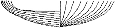
Fig. 4 — Body plan of the Athena hull.
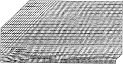
Fig. 5 — Top view of the panelling of the athena hull and the free surface near the hull.

Fig. 6 -Contours of the computed free-surface elevation for the Athena hull at F = 0.48. Solid lines indicate positive nondimensional wave elevation Z/F2= 0.005j for j = 1,2, etc. Dashed lines indicate negative wave elevation Z/F2= -0.0005j for j = 1,2, etc. The zero contour level is not drawn. (b) Measured
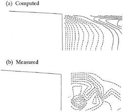
Fig. 7 -Contours of the Kelvin wave pattern near the transom stern of the Athena hull at F = 0.48. (a) Contours of the computed wave elevation. (b) Con-tours of the measured wave elevation. [Measured data from (12).] T he contour levels are the same as in Fig. 6.
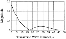
Fig. 8 - Amplitude of the free-wave spectrum from a pair of transverse wave cuts at 1.15 and 1.20 ship lengths aft of the midship section of the Athena hull for F = 0.48.

Fig. 9—Contours of the computed free-surface elevation for the Athena hull at F=0.4. Solid lines indicate positive nondimensional wave elevation Z/F2=0.005j for j=1, 2, etc. Dashed lines indicate negative wave elevation Z/F2=−0.005j for j=1, 2, etc. The zero contour is not drawn.
Froude number 0.414 are shown in Fig. 13 and Fig. 14a. The computed contours near the transom are compared with the corresponding contours obtained from measurements in Fig. 14. (In Fig. 14b, the contours immediately behind the transom are computed, not measured, since no measurements were obtained in this region.) From Fig. 14b it appears that the peak behind the stern is nearly in the correct position. The measured contours of the wave elevation in Fig 14b show a sharp gradient of the wave elevation that starts approximately 0.1 ship length aft of the stern and lies along a ray at about the Kelvin angle away from the center plane. In the computed contours of Fig. 14a there is a corresponding surface height gradient, but is not as sharp. The peak of the computed free-surface elevation here corresponds to level 0.08F2 whereas the measured wave height corresponds to level 0.085F2. A comparison of the amplitude of the free-wave spectrum obtained from computed wave elevations along transverse wave cuts and from measured wave elevations is presented in Fig. 15. The wave resistance computed from the amplitude of the wave spectrum shown in this figure is 0.0018, which is lower than the value of 0.0024 obtained from experimental data.
For Froude number 0.25 contours of the computed free-surface height are shown in Figs. 16 and 17a. The corresponding amplitude of the free-wave spectrum is plotted in Fig. 18. A close-up comparison of the contours of computed and measured wave elevation near the stern of Model 5415 at Froude number 0.25 is provided in Fig. 17. For this speed, measurements are available in the region immediately behind the stern. The positions of the computed and measured peaks behind the stern agree fairly well. Outside the area immediately behind the stern, as is the case for the higher speed, there is a sharp gradient in the measured wave elevation along a line starting
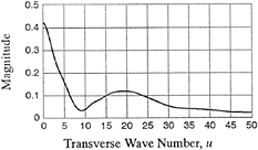
Fig. 10—Amplitude of the free-wave spectrum obtained from a pair of transverse wave cuts at 1.15 and 1.20 ship lengths aft of the midship section of the Athena hull for F=0.4.
at the stern and radiating downstream from the hull at approximately the Kelvin angle. The large gradient is also present in the computed results, but it is not as sharp. At the peak elevation near the sharp gradient, the computed nondimensional free-surface height is 0.08 F2. Except for a very small area where the measured elevation is higher, this is the nondimensional wave height of the highest measured contour level plotted. The wave resistance computed from the magnitude of the wave spectrum is 0.00042, which is higher than the value of 0.00037 obtained from experimental data.
If paneling behind the stern is placed on the mean free-surface level rather than on the cylindrical surface surface extending downstream from the hulltransom intersection and if no strips of wake panels originating at the transom are used, then a different solution is obtained. In this case finite differencing to set the free-surface depth and slope immediately behind the stern is based on the potential solely at the centroids of free-surface panels and thus excludes the potential on the hull. Contours of the wave elevation near the stern for Froude numbers 0.25 and 0.414 are shown in Figs. 19 and 20. These are to be compared with the previous results depicted in Figs 17a and 14a, respectively. There is a visible difference in the contours. There is less of the sharp gradient that is seen in the contours of the experimental measurements. This difference is more obvious for the lower speed. Corresponding plots of the amplitude of the free-wave spectrum are given in Figs. 21 and 22. There is not much difference at Froude number 0.414.
CONCLUSION
It has been shown that it is possible to linearize the wave resistance problem about a surface that originates at the intersection of the hull and a transom

Fig. 11 - Body plan of Model 5415.

Fig. 12 -Top view of the paneling on Model 5415 and on the surrounding free surface.
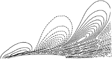
Fig. 13 - Contours of the computed Kelvin wave pattern for Model 5415 at F = 0.414. Solid lines indicate positive nondimensional wave elevation Z/F2 = 0.005j for j = 1, 2, etc. Dashed lines indicate negative wave elevation Z/F2 = -0.005j for j = 1,2, etc. The zero contour level is not drawn.

Fig. 14 - Contours of the free-surface elevation near the transom stern of Model 5415 at F = 0.414. (a) Contours of computed wave elevation. (b) Contours of measured wave elevation except aft of the transom where contours of computed wave eleva-tion are presented (and are identical to the corre-sponding contours in (a)). Contour levels are the same as in Fig. 13

Fig. 15—Comparison of the amplitude of the free-wave spectrum for Model 5415 at F=0.414 obtained from a pair of computed transverse wave cuts (—) and from experiments (▲).
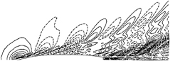
Fig. 16—Contours of the computed free-surface elevation for model 5415 at F=0.25. Solid lines indicate positive wave elevation Z/F2=0.005j for j= 1,2, etc., and the dashed lines, negative wave elevations Z/F2=–0.005j for j=1,2, etc. The zero contour is not drawn.
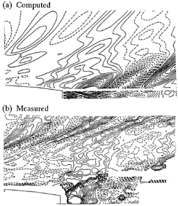
Fig. 17—Contours of the free-surface elevation near the stern of model 5415 at F=0.25 (a) Contours of computed wave elevation. (b) Contours of measured wave eleveation. Contour levels are the same as in Fig. 16.

Fig. 18—Amplitude of the free-wave spectrum for Model 5415 at F=0.25 obtained from a pair of computed transverse wave cuts (—) and from experiments (▲).
stern and which extends downstream from this intersection. The computed wave height is different from the wave height obtained using a model in which panels behind a transom stern are placed on the mean free-surface level and the transom is left open. For the few results presented here, some features present in experimental results show up more clearly when panels behind the stern are placed on the surface originating at the hull-transom intersection.
To compute the solution of the wave resistance problem, we have modified an existing Rankine singularity code that had been based on the use of distributions of sources and dipoles on the mean free-surface level. The finite-differencing scheme in the code was replaced by one in which analytic differentiation and collocation point shifting are used to enforce the radiation boundary condition. In so doing free-surface integrals have been replaced by a combination of free-surface and hull-waterline integrals. The hull-waterline integrals are analogous to those customarily seen in Havelock singularity methods only in that similar mechanisms are used to arrive at them; they are otherwise completely different. The wave height appears to be calculated more accurately by using this scheme than by using the scheme in the original code.
Difficulties can be expected in this method when the wave slope is enforced at a transom stern. Several causes can be singled out. First, obtaining the hull slope is problematic since there is typically a rapid variation in the hull shape at the stern. Second, developing an accurate numerical scheme that enforces the slope on a curved surface is complicated. Here part of the latter problem has been eliminated by using a cylindrical surface beneath the mean free-surface level without longitudinal variation in depth downstream of the hull-transom intersection.
Further developments might be made. The first involves putting panels behind a hull-transom intersection on a curved surface that rises toward the mean free-surface level. This was tried, but anomalies in the contours of the computed wave elevation directly behind the transom led to the simpler approach of putting panels on a cylindrical surface originating at the intersection. Perhaps the linearization scheme should be reexamined, or perhaps the accuracy to which higher derivatives of the potential due to source and dipole distributions on curved surfaces can be computed should be reevaluated. As a second refinement, the nonlinear zero-pressure Kutta condition, Bernoulli 's equation with the pressure set to atmospheric pressure, could be satisfied at the transom stern. This nonlinear Kutta condition should be used in conjunction with a varying depth in the surface originating at the hull-transom intersection about which the free-surface boundary conditions are linea-
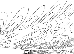
Fig . 19 - Contours of computed free-surface elevation for Model 5415 hull at F = 0.25. Paneling behind the transom stern has been placed on the mean free-surface level. Finite differencing at the upstream end of strips of panels originating at the stern involves the disturbance potential only at the centroids of free-surface panels instead of at the centroids of neighboring free surface and hull pan-els. Solid lines indicate positive wave elevation Z/F2 = 0.005j forj = 1,2, etc. and dashed lines, neg-ative elevation Z/F2= -0.005j forj = 1,2, etc. The zero contour level has not been drawn.
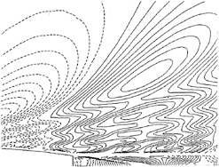
Fig. 20 - Contours of computed free-surface elevation for Model 5415 hull at F = 0.414. Paneling aft of the transom stern has been placed OII the mean free-surface level. Finite differencing at the upstream end of strips of panels originating at the stern involves the disturbance potential only at the centroids of free-surface panels instead of at the centroids of neighboring free-surface and hull panels. The contour levels are the same as in Fig. 19.

Fig. 21 - Amplitude of the free-wave spectrum obtained from a pair of computed transverse wave cuts at 1.15 and 1.20 ship lengths aft of the midship of Model 5415 Froude number 0.25 (—) and the corresponding spectrum obtained from experimen-tal data (▲). Paneling aft of the transom stern has been placed on the mean free-surface level. Finite differencing at the upstream end of strips of panels originating at the stern involves the disturbance po-tential only at the centroids of free-surface panels instead of at the centroids of neighboring free-surface and hull panels.
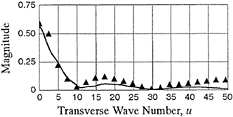
Fig. 22—Amplitude of the free-wave spectrum obtained from a pair of computed transverse wave cuts at 1.15 and 1.20 ship lengths aft of the midship section of Model 5415 at F=0.414 (—) and the corresponding spectrum obtained from experimental data (▲). Paneling aft of the transom stern has been placed on the mean free-surface level. Finite differencing at the upstream end of strips of panels originating at the stern involves the disturbance potential only at the centroids of free-surface panels instead of at the centroids of neighboring free surface and hull panels.
rized. The combination may be especially important for deep transoms.
Although, according to Lechter (6), the method of collocation point shifting and analytic differentiation may break down at low Froude numbers, several enhancements might be made to the Rankine singularity method that was used to obtain numerical approximations to free-surface potential flows. They are related to the more general problem of calculating the linearized free-surface potential flow near arbitrarily shaped ships advancing into calm water. The first would be to eliminate the finite differencing at the hull waterline. This would eliminate all finite differences except those at the hull-transom intersection. Second, the relationship between free-surface paneling and collocation point shifting should be clarified. When a second small longitudinal shift downstream is used, damping is introduced into the wave pattern. Further, a more or less rectangular grid of panels on the free surface damps the waves in the Kelvin wave pattern more than the arrangement used in this paper, in which the computational free-surface domain is swept back at a 45-degree angle. The effect is most noticeable in the diverging waves seen in contour plots. Finally, it might be useful to consider whether something similar to the DtN exact boundary condition of Keller and Givoli (14) could be used for the outer boundaries of the computational domain to handle the boundary conditions there more accurately and to reduce the size of the computational domain.
ACKNOWLEDGMENT
This work was supported in part by the Applied Hydromechanics Research program of the Applied Research Division of the Office of Naval Research.
REFERENCES
1. Lindenmuth, W.T., Ratcliffe, T.J., and Reed, A.M., “Comparative Accuracy of Numerical Kelvin Wake Code Predictions—‘Wake-Off'”. DTRC Ship Hydromechanics Dept. R & D Report DTRC-91/004, 1991, 257+xiv p.
2. Cheng, B.H., “Computations of 3D Transom Stern Flows,” Proc. Fifth International Conference on Numerical Ship Hydrodynamics, National Academy Press: Washington, DC, 1989, pp. 581–592.
3. Reed, A., Telste, J., and Scragg, C., “Analysis of Transom Stern Flows,” Proc. Eighteenth Symposium on Naval Hydrodynamics, National Academy Press: Washington, DC, 1990, pp. 207–220.
4. Nakos, D.E. and Sclavounos, P.D. “Kelvin Wakes and Wave Resistance of Cruiser and Transom Stern Ships, ” Journal of Ship Research, to appear.
5. Tulin, M.P. and Hsu, C.C., “Theory of High-Speed Displacement Ships with Transom Sterns,” Journal of Ship Research, Vol. 30, No. 3, 1986, pp. 186–193.
6. Lechter, J.S., “Properties of Finite-Difference Operators for the Steady-Wave Problem, ” Journal of Ship Research, Vol. 37, No. 1, March 1993, pp. 1–7.
7. Jensen, P.S., “On the numerical radiation condition in the steady-state ship wave problem,” Journal of Ship Research, Vol. 31, No. 1, March, 1987, pp. 14–22.
8. Eggers, K., Sharma, S.D., and Ward, L.W., “An Assessment of Some Experimental Methods for Determining the Wavemaking Characteristics of a Ship Form,” SNAME Transactions, Vol. 75, 1967, pp. 112–57.
9. Sharma, S.D., “A Comparison of the Calculated and Measured Free-Wave Spectrum of an Inuid in Steady Motion,” Proc. Int'l Seminar on Theoretical Wave-Resistance, Vol 1, University of Michigan, Ann Arbor, 1963, pp. 203–272.
10. Dawson, C.W., “A Practical Computer Method for Solving Ship-Wave Problems,” Proc. Second International Conference on Numerical Ship Hydrodynamics, Univ. of California: Berkeley, California, CA, 1977, pp. 30–38.
11. Sclavounos, P.D. and Nakos, D E., “Stability of Panel Methods for Free-Surface Flows with Forward Speed, ” Proc. Seventeenth Symposium on Naval Hydrodynamics, National Academy Press: Washington, DC, 1988, pp. 173–93.
12. Jenkins, D.S., “Resistance Characteristics of the High Speed Transom Stern Ship R/V Athena in the Bare Hull Condition, Represented by DTNSRDC Model 5365, ” Ship Performance Dept. R & D Report DTNSRDC-84/024, 1984, 59+ix p.
13. Ratcliffe, T.J. and Lindenmuth, W.T., “Kelvin Wake Measurements Obtained on Five Surface Ship Models,” DTRC Ship Hydromechanics Dept. R & D Report DTRC-89/038, 1990, 88+x p.
14. Keller, J.B. and Givoli, D., “Exact Non-reflecting Boundary Conditions,” Journal of Computational Physics, Vol. 82, 1989, pp. 172–192.


