
Navier-Stokes Computations of Ship Stern Flows: A Detailed Comparative Study of Turbulence Models and Discretization Schemes
G.B.Deng, P.Queutey, and M.Visonneau
(Ecole Centrale de Nantes, France)
ABSTRACT
A fully elliptic numerical method for the solution of the Reynolds Averaged Navier Stokes Equations is applied to the flow around the HSVA Tanker. The weaknesses of the simulation are analysed by comparing several discretisation schemes and grids as well as several turbulence models. Grid refinement in the near wake or application of new accurate discretisation schemes have a little effect on the quality of the solution in the wake. Systematic comparisons of various turbulence models and numerical experiments suggest that the solution is essentially affected by a too high level of turbulence viscosity in the core of the longitudinal vortex.
NOMENCLATURE
Variables
|
(x,y,z) |
cartesian coordinates |
|
U |
average velocity vector |
|
p |
pressure |
|
t |
time |
|
Re |
Reynolds number |
|
uu |
Reynolds stress tensor |
|
k |
turbulent kinetic energy |
|
ε |
rate of turbulence dissipation |
|
I |
Identity tensor |
|
vT |
eddy viscosity |
|
Cμ,Cε1, Cε2,σk,σε |
k-ε coefficients |
|
Reff, Rk, Rε |
effective Reynolds numbers |
|
G |
production |
|
ξ,η,ζ |
curvilinear coordinates |
|
u,v,w |
contravariant components of the velocity |
|
U,V,W |
cartesian components of the velocity |
|
J |
jacobian |
|
|
j component of the contravariant vector bi |
|
gij |
contravariant metric tensor |
|
SU1 |
source term for the momentum equations |
|
Sk |
source term for the k transport equation |
|
Sε |
source term for the ε transport equation |
|
CNB |
influence coefficients at point C |
|
A,B |
normalized convective velocities |
|
ÛC |
pseudo-velocity at point C |
Operators
|
Div |
divergence |
|
|
gradient |
|
|
laplacian |
|
|
transposed gradient |
1.
INTRODUCTION
Advances in numerical solution methodology along with increased computer storage and speed have made it possible to seek numerical solutions of the three-dimensional Reynolds Averaged Navier Stokes Equations (RANSE) for moderately complex ship hulls. With the development of computers, wind tunnel or towing tank experiments are no more the only way to get information on ship performances and CFD tools appear to be able to generate an overwhelming amount of information on the flow with a level of details and flexibility which seems out of reach of a reasonable experimental approach. These computations are nevertheless mostly confined to double models, in which wave effects are absent, to
bare hulls without appendages or propulsors and conducted at laboratory Reynolds numbers. However, even for these simple configurations, it is crucial to locate as accurately as possible the limitations of numerical simulations in order to know (i) which level of details can be reasonably captured by a CFD tool, (ii) what are the leading weaknesses of the simulation and (iii) how to improve the accuracy of the numerical prediction.
From that point of view, the so-called HSVA tanker is known as the best documented test case among all the available experimental ship flow data bases. It is why it was chosen as one of the two testcases of the 1990 SSPA-
CTH-IIHR Workshop on Ship Viscous Flow which was held at Goteborg [1]. Some nineteen organizations coming from twelve countries participated in the Workshop and all of them calculated the first test case i.e. the flow around the HSVA tanker at the laboratory Reynolds number Re=5.0 106 on which this paper will be entirely focussed.
Despite its seemingly geometric simplicity, the flow around this hull is rather complex. As the flow progresses along the hull, the geometry of the body gradually forces the boundary layer to pack in an area whose girthwise dimension decreases, implying a progressive convergence of the streamlines in some regions of the hull. Continuity requires a large normal velocity, a strong thickening of the boundary layer occurs often associated to the birth of a longitudinal vortex motion which is slowly relaxed in the wake at large distances downstream from the ship.
A more detailed understanding of the flow is provided by the visualisation of the limiting streamlines (Figure 1 from [1]), actually the print of the flow on the hull; it clearly indicates the existence of a well defined line of convergence located just beyond the keel plane of symmetry. It is also quite clear that the behaviour of the limiting streamlines is complex since two convergence lines are visible. The first one (S1 line) is S-shaped and demarcates a vertical wall flow region and a small zone of flow reversal. The second convergence line (S2 line) is located just beyond the keel plane of symmetry and joins the S1 line at the end of the hull. Consequently, since this region seems to be characterized by a rapid normal variation of the velocity orientation from the wall to the so-called logarithmic region, it is plausible to think that such a complex three-dimensional behaviour can be hardly simulated by a wall function approach which cannot account for the high twist angle (>90º) between the wall flow and the external streamlines directions.
Even more interesting are the measurements of the pressure and velocity components made at several cross-sections. Figs 2-a-b-c from [1] show the axial velocity contours at several locations, namely, x/L=0.908, 0.976 and 1.005. The longitudinal velocity contours indicate a very characteristic “hook” shape in the central part of the wake correlated with the core of the longitudinal vortex. This small region is characterised by a nearly uniform U component, a linear variation of the vertical component W preceding a maximum and again an “hook” shape of the pressure contours. These features confirm the existence of an intense longitudinal bilge vortex emanating from the hull and leads us to classify the HSVA tanker as an U-shaped hull rather than a V-shaped hull for which the longitudinal vortex is far more intense and does not create this very characteristic hook shape of the longitudinal velocity contours.
The Goteborg workshop's results indicated that great progress has been made through the development of methods based on the Reynolds-Averaged Navier Stokes Equations. These methods generally simulate the gross features of the wake and predict the shape and location of the velocity contours with reasonable accuracy even on the rather coarse meshes recommended for the simulations. Nevertheless, neither the central part of the wake with this hook shaped velocity contour nor the entire wall flow behaviour can be captured by the methods presented at this time.
The description of this phenomena could be of crucial importance for the design since the designer's task is to devise the best hull geometry leading to improvments to propulsive efficiency through better hull form/propeller matching. This is often a compromise between V-shaped stern sections which are associated to lower viscous resistance and less intense longitudinal bilge vortex and U-shaped stern sections for which the more intense longitudinal bilge vortex create an higher propulsive efficiency which partly compensates for the higher resistance. It is therefore fundamental to determine if the solution of the RANSE enables us to distinguish between the flows associated to U-shaped or V-shaped geometries without ambiguity.
During the workshop, several hypotheses were put forward to explain the incapability of the RANSE-based methods to describe accurately the central part of the bilge vortex. Two types of explanations may be evocated, the first one favouring the discretization inaccuracies and the second one emphasizing the weaknesses of the turbulence modelisation.
It is sensible to stress the numerical inaccuracy since the threedimensional grids are often too coarse to capture the details of the flow especially if we consider that most of the discretisation schemes are only first order accurate when the flow is dominated by the convection and not aligned with the coordinate lines. The numerical solution produced by such discretisation schemes is always too diffusive and local inhomogeneities such
as this hook shape are filtered by a too high artificial viscosity.
On the other hand, it is reasonable to stress the weaknesses of the classical turbulence modelisation for this class of stern flows. As it was pointed out by V.C.Patel in [2], the turbulence in stern flows seems to behave in a very specific way. Let us compare with him the behaviour of the measured kinetic energy k plotted in outer variables, with U0 and δ as scales of velocity and length for two different flows, a thick boundary layer stern flow around the SSPA hull and a traditional flat plate flow (Fig. 3 from [2],[15]). The measurements for the strong thick boundary layer indicate a two layer structure, leading V.C.Patel to wonder if a single set of scaling parameters is adequate to modelize this flow. The outer zone is actually characterized by a lower level of the turbulence intensity, meaning that the conventional turbulence model might generate again a too diffusive flow.
Then, the conjecture could be stated in these terms. What is the respective importance of the artificial viscosity compared with the likely inadequacy of the turbulence modelling? Actually, these aspects are strongly tied up if we think that the turbulence numerically produced by the discretised k-ε transport equations is somewhat modified by various numerical inaccuracies among which might be quoted the discretisation errors, an unsufficient level of coupling between the source terms of the turbulence transport equations or an unsatisfactory level of convergence for the nonlinearities. This is why some authors consider it safer to use a simpler 0 equation turbulence model like a Baldwin-Lomax model.
The aim of this paper can be summarised as follows: (i) to determine what is the respective weight of the numerics compared to the turbulence modelisation for this class of stern flows, (ii) to show what has to be improved in the future to use the RANSE based methods as a reliable design tool in the naval architecture context.
This paper is outlined as follows. In section 2, the alternative curvilinear formulations are described as well as the turbulence models used in the present study. Section 3 is devoted to a brief survey of the two numerical methods being the subject of comparisons. In section 4, the conditions of the computations are described and the relative influence of turbulence models and numerical approaches upon the simulation is investigated. Some concluding remarks are mentionned in Section 5.
2.
EQUATIONS
2.1
The Basic Equations
We consider the equations of motion in cartesian (x,y,z) coordinates for incompressible flows. The exact RANSE of continuity and momentum of the mean flow in dimensionless form are given by equations (2.1), (2.2) and (2.3):
divU=0 (2.1)
(2.2)
(2.3)
U,p and uu are respectively the velocity vector, the pressure and the Reynolds stress tensor. The resulting turbulent closure problem is solved by means of the classical k-ε turbulence model in which the Reynolds stress is linearly related to the mean rate of strain tensor through an isotropic eddy viscosity as follows:
(2.4)
If the k-ε turbulence model is used, the eddy viscosity vT is classically given by:
(2.5)
where the adimensional turbulent kinetic energy k and its dimensionless rate of dissipation ε are governed by the following transport equations:
(2.6)
(2.7)
where G is the turbulence generation term:
G=vT![]() U:(
U:(![]() U+
U+![]() TU) (2.8)
TU) (2.8)
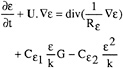
The effective Reynolds numbers Rk, Rε, Reff have been defined by:
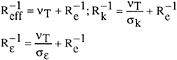
(2.9)
Unless specified, the constants in the previous equations are taken to their standard values (2.10):
In order to avoid the wall function approach, several near wall k-ε models are compared in this study. For the sake of brevity, the details concerning their implementation, which can be found in [ 4], [13] and [14], are omitted here. For a significant increase of numerical troubles and computing time (because the integration is carried out to y+≈1), the delicate problem of the three-dimensional specification of the log-law, dealt with only in [5], is avoided.
The algebraic Baldwin-Lomax model [6] is also evaluated because it is less expensive in terms of CPU effort and rate of convergence.
2.2
The Equations In The Transformed Coordinate System
For hydrodynamic applications, a numerical coordinate transformation is highly desirable in that it greatly facilitates the application of the boundary conditions and transform the physical domain in which the flow is studied into a parallelepipedic computational domain ![]()
The partially transformed RANSE are given by the following relations in a fully conservative developped form. The contravariant components of the velocity are defined by ![]() and the physical cartesian components by
and the physical cartesian components by ![]()
(2.11)
(2.12)
with ![]() =U,V,W,k,ε where:
=U,V,W,k,ε where:
(2.13)
while ![]() =Reff if
=Reff if ![]() =U,V,W;
=U,V,W;
![]() =Rk if
=Rk if ![]() =k;
=k;
![]() =Rε if
=Rε if ![]() =ε
=ε
Also,
The alternative convective form needs to be introduced (2.14):

(2.14)
where:

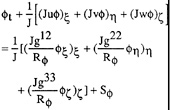
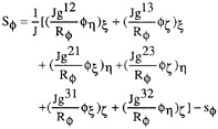
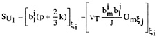
The additional source terms contain classically the pressure gradients and the turbulence contributions:
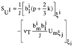
(2.15)

(2.16)
Endly, the metric coefficients involved in the transformation are given. They are the contravariant base, {bi}, normalized by the Jacobian, J, of the transformation and the metric tensor g:

gij=J−2bibj; (2.17)
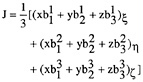
(2.18)
The convective form needs the functions fj which can be seen as purely geometrical convective coefficients or defined as stretching functions:
(2.19)
3.
THE NUMERICS
In order to clarify the role played by the accuracy of the discretisation schemes, two approximation methods are evaluated. Before detailing the differences, let us first recall their common characteristics. For each of them, a cell-centered layout is used in which pressure, turbulence and velocity unknowns share the same location. This strategy simplifies coding and leads to significant savings in computational time and storage. Even if a steady solution is looked for, a local time step ensuring a fixed amount of diagonal dominance with respect to the momentum equations, is devised to accelerate the convergence towards the steady state. Endly, the momentum and continuity equations are coupled through the well known (one step) PISO procedure already detailed in [7].
3.1
Method 1
The Convection Diffusion Schemes
The momentum equations are written down under their convective form (2.14). When the Multi-exponential scheme is used, the normalized transport equation is splitted as follows :
2 A ![]() ξ−
ξ−![]() ξξ=D2−(R
ξξ=D2−(R ![]() t+
t+![]() ) (3.1)
) (3.1)
2 B ![]() η−
η−![]() ηη=D1−(R
ηη=D1−(R ![]() t+
t+![]() ) (3.2)
) (3.2)
where D1 and D2 are defined as:
−D1=2A![]() ξ−
ξ−![]() ξξ, (3.3)
ξξ, (3.3)
−D2=2B![]() η−
η−![]() ηη, (3.4)
ηη, (3.4)
Using an exponential scheme for every equation and summing gives the so-called multi-exponential scheme:
(CU+CD+CN+CS)![]() C=CU
C=CU![]() U+CD
U+CD![]() D +CN
D +CN![]() N+CS
N+CS![]() S−(R
S−(R![]() t+
t+![]() ) (3.5)
) (3.5)
where
(3.6)
The multi-exponential scheme is very similar to the hybrid scheme. Its coefficients are always positive. It is second order accurate when the cell Reynolds numbers A, B are small, and it behaves as an upwind scheme when A, B dominate. Although the accuracy is similar to that of the hybrid scheme, this scheme is preferred since the coefficients resulting from this discretization vary smoothly, this factor is favorable for convergence.
The Uni-exponential scheme is a skew upwind exponential scheme designed to decrease the numerical diffusion occuring in the previous scheme when the flow is not aligned with the grid lines. The idea is briefly outlined below for a 2D equation. After normalisation, the 2D transport equation can be written as:
(3.7)
where s is the local advection direction. The first term can be expressed by an exponential discretization, while other second derivatives are discretised by centered differences. A parabolic interpolation fonction is used to express the intermediate values ![]() U and
U and ![]() D in terms of dependent variables, for instance:
D in terms of dependent variables, for instance:
(3.8)
which results in a 9 points formula.
(3.9)
Extension to the 3D case is straightforward and a 27 points formula is obtained. The 3D Uni-exponential scheme is not a positive scheme, but this fact does
not induce any troubles, neither in the convergence, nor in the monotony of the solution. Nevertheless, this scheme is only first order accurate when the flow is dominated by a balance between convection and pressure gradient.
The Continuity Equation
The fully conservative formulation is retained. The discretised form is a balance between unknown mass fluxes:
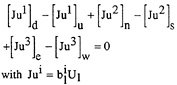
(3.10)
On the both sides of the control volume interface, the discretised momentum equations are available and can be written as:
(3.11)
where the contributions of neighbouring points and source term (except the pressure gradient) are accumulated into the pseudo-velocity ![]() (C).
(C).
We must now reconstruct the contravariant velocity components ui needed at the control volume interfaces to enforce continuity and to avoid the chequerboard pressure oscillations.
(3.12)
Instead of interpolating U1 from available neighbouring values of the same species, U1 is linked to other dependent variables through a local ‘pseudo-physical' approximation of momentum equation at the control volume interface [8].
(3.13)
A linear interpolation (in the computational domain) is used to build ![]() and
and ![]() but the pressure gradient is rediscretised at the respective interface. This is why this reconstruction is called “pseudo-physical”. Using the relation (3.12), the contravariant components are now given by:
but the pressure gradient is rediscretised at the respective interface. This is why this reconstruction is called “pseudo-physical”. Using the relation (3.12), the contravariant components are now given by:

(3.14)
Using relation (3.13), the mass fluxes are gathered in (3.10) to provide a pressure-pseudo-velocity equation which does not admit chequerboard oscillating solutions.
3.2
Method 2
The Convection Diffusion Scheme
The major drawback of the previous discretisation schemes comes from the fact that the local variations of the convection or diffusion coefficients as well as the source term are not accounted for in the influence coefficients. The CPI (Consistent Physical Interpolation) scheme, based on a fully conservative formulation of the momentum equations, was proposed recently by the authors to remedy this weakness [9]. Its name stems from the fact that the fluxes are reconstructed from auxiliary (momentum) equations which are rediscretised at the interfaces of the control volume. This discretisation provides a “dynamical interpolation formula” linking the interfacial unknowns to the neighbouring cell-centered unknowns. For instance, the 2D reconstruction formula for the unknown u at the interface e is given by:

(3.15a,b)
with:

(3.16a,b)
The pseudo-velocities ![]() are no more interpolated from the available neighbouring
are no more interpolated from the available neighbouring ![]() like in the previous approach. They are linked to the surrounding velocities UNB through a discretisation of an auxiliary momentum equation. This is why the CPI approach is a generalisation of the previous recontruction: (i) this is a physical reconstruction, (ii) this technique is applied not only to the continuity equation but also to the momentum equations. For the sake of compacity, the details concerning the stencil and the
like in the previous approach. They are linked to the surrounding velocities UNB through a discretisation of an auxiliary momentum equation. This is why the CPI approach is a generalisation of the previous recontruction: (i) this is a physical reconstruction, (ii) this technique is applied not only to the continuity equation but also to the momentum equations. For the sake of compacity, the details concerning the stencil and the
discretisation scheme which can be found in [9], are omitted here.
After elimination of the interfacial unknowns and combination of the various fluxes, the CPI method yields a stable second-order accurate twenty-seven point stencil in the three-dimensional case.
The Continuity Equation
The available reconstructed mass fluxes are gathered into the continuity equation which provides a new pressure-pseudo velocities equation.
4.
THE RESULTS
The Grid Topology
The flow domain covers 0.5<x/L<3, L being the length of the ship; rS<r/L<1. Starting from an a priori specified surface grid distribution, a volumic mesh is generated using a transfinite interpolation procedure. A new O-O topology is preferred to the previous H-O grid topology [7], This new topology enables us to optimize the number of points describing the hull and makes it possible a better description of the near wake flows. The fact that no a priori grid line is aligned with the dominant flow direction could appear as a disadvantage. Actually, since the fully elliptic RANSE are retained here, and since no particular anisotropic splitting is involved in the discretisation schemes, we think that the results are not too penalised by this choice. At the very most may we fear a slight increase of false diffusion in some parts of the flow domain. This likely drawback is largely compensated for by the fact that this fully body fitted grid allows a correct handling of the propeller boss, which was not possible with x=x(ξ) grids used in [7].
The Boundary Conditions
Inlet velocity profiles (ξ=1) are generated in accordance with the method of Coles and Thompson [10] which needs the specification of δ, Uτ and Qe. These values are estimated from the specified data [11], [12] where:

in order to match the solution to the measured data at X/L=0.646. However, it is felt that the influence of inlet conditions is forgotten at the stations on the afterbody and in the wake.
Neumann conditions are used for the planes of symmetry (ξ=ξmax, ζ=1 and ζ=ζmax). No slip conditions is enforced on the hull (η=1) and free stream conditions (U=1, V=W=0) are applied at the outer surface (η=ηmax). Velocity profiles are slightly modified to enforce the global mass continuity constraint; hence, linear extrapolation is used for the extraneous pressure boundary conditions on all the surfaces limitating the flow domain instead of the usual Dirichlet condition p=0.
The First Results
Computations with Method 1 associated to a two-layer k-ε model [4] are performed on a 80×40×51 fully body fitted grid based on an O-O topology described before (Grid I). Figure 4 shows a perspective view of this grid. The clustering of the grid close to the hull is such that the boundary layer is always described by more than 25 points, the first point being located in the viscous sublayer (y+=1). The longitudinal pressure distributions are presented in figs. 5a-b. A very good agreement with the experimental results is observed on the waterline while the pressure distribution on the keel line presents the same trends as in [7], i-e an overestimation of about 40% near x/L=0.875. However, the spike that was present at X/L=0.90 in our previous computations [ 7] has disappeared here.
Girthwise pressure distributions at several x-stations (figs 6a-b-c) exhibit the same trends as in [7].
The computational and experimental skin friction lines on the hull surface are presented in figs 7a-b. They both indicate that the flow close to the stern separates along an S convergence line (S1 line). The excellent agreement of the results with visualisation data is due to the eviction of the wall function approach associated to the use of a fully body fitted grid on which the propeller boss can be correctly accounted for. Nevertheless, the convergence line present in the visualisation data near the keel line (S2 line) is completely missed by the computations. The calculated skin friction lines go up from the keel line and cross this region without any distortion.
The axial velocity contours at the propeller plane (x/L=0.976) are presented in figs 8a-b-c. Two convection-diffusion schemes have been employed to generate the computational results; the first one is the multi-exponential scheme based on a 7 points stencil and the second one is the uni-exponential one which leads to a 27 points stencil. They are both first order accurate when the flow is dominated by a balance between convection and pressure forces but the last one is preferred because the extraneous
corner points enable a more accurate representation of the convective direction and leads to a reduction of the directional numerical viscosity. Nevertheless, even if the results are improved when the Uni-exponential scheme is used—the axial velocity contours have a bulge on a level near the propeller centerline—the characteristic hook shape present in the measured velocity contours is not found by the computations.
Endly, the velocity components U,V,W as well as pressure data are compared more extensively in figs 9–10–11. For each series of plots, the evolution is considered with respect to y for several depths z=cste. Here again, the calculations exhibit a correct agreement with the data except in the region close to the core of the longitudinal vortex. The experimental U profiles are characterised by a non-monotonicity which is forgotten by the computations. The maximum of W profiles is underestimated in the computations, indicating that the calculated longitudinal vortex is less intense than its experimental counterpart.
The results of these simulations are in good agreement with the experimental measurements. The gross features of the wake such as the thin shear layer near the keel, the accumulation of low speed flow in the middle part of the hull and the related occurence of a longitudinal vortex are correctly captured by the computations. However, the simulated flow seems more regular than the experimental one and some very specific details, such as the low speed region in the vicinity of the propeller disk associated to the hook-shaped velocity contours, appear filtered by the simulation. Actually, the computed flow looks like the flow around a slender hull, which makes questionable the use of the results of simulations to improve the geometry via an interactive design process.
Influence of Discretisation Errors
Therefore, it is necessary to identify the parameters which have a dominant influence on the quality of the simulation for such hulls. As pointed before, the influence of the discretisation scheme does not seem negligible. In order to clarify the degree of importance of discretisation errors, two categories of tests are conducted.
Test 1
For the first test, the usual methodology based on the Uni-exponentiel scheme and a Baldwin-Lomax model is retained (Method 1). The computations are performed on a refined mesh (121×61×60) (Grid II) based on the same O-O topology. The clustering of discretisation points is such that about twice more points per direction are present into the propeller disk region. Figure 12 shows the girthwise Cp distribution for three locations, namely, x/L=0.64, 0.87 and 0.94. For the first two stations, no spectacular improvment can be noticed. However, the strong gradient near the keel plane of symmetry is better captured on the finer grid. Figure 13 presents a visualisation of skin-friction lines on the hull which is not noticeably different from the one obtained on Grid I. Figure 14 shows the longitudinal velocity contours in the propeller disk. Again, no evident improvment can be noticed so that it seems that the results are more or less grid independant.
Test 2
In order to assess the influence of the discretisation errors, a new convection diffusion scheme (CPI) leading to a totally new methodology, has been applied to this problem (Method 2). A Baldwin-Lomax turbulence model is again used here and the computations are performed on Grid I. Figures 15–16 show the girthwise Cp distributions and the wall flow which are not significantly different from the results obtained with Method 1 on Grid I. Figure 17 shows the axial velocity contours at x/L=0.976. The bulge is now slightly more developped but the innermost contours do not reveal any hook-configuration.
Several numerical tests have been performed to evaluate the weight of numerical inaccuracies. Neither the computation on a refined grid, nor the use of a new discretisation method, have improved the computed simulation in the near wake. As a matter of fact, even if the global characteristics are slightly improved, the characteristic hook-shaped contours are not predicted in the propeller disk region. These numerical tests indicate that (i) the solution is more or less grid independent on Grid I, (ii) the simulated flow is too diffusive, (iii) the turbulence modelisation plays a major role in the mechanisms giving birth to these uneven vortex features.
Influence Of The Turbulence Modelisation Errors
To evaluate the influence of the classical newtonian turbulence models, the Baldwin-Lomax model has been compared to several k-ε models (Chen & Patel [4], Nagano & Tagawa [13], Deng & Piquet [14]) for which the wall function approach is always discarded. For the sake of brevity, the results are just mentionned and not analysed in detail. The k-ε models should be more accurate since the eddy viscosity depends on the two quantities k and ε which are obtained by solving transport equations. However, the supremacy of the k-ε models over the algebraic Baldwin-Lomax model is not demonstrated for this class of flows. As it was pointed out in [1], the aforementionned tested models produce
essentially the same too diffusive flow, especially in the near wake region.
In order to get an idea of what has to be modified to improve the simulation, a last “heretic” computation has been performed by reducing the level of the eddy viscosity by a factor 2.5 in the core of the longitudinal vortex. Figure 18 shows the axial velocity contours at x/L=0.976. The hook-shaped configuration is now captured and figs 19a-b confirm the very good agreement between this computation and the experiments. The U component profiles are non-monotonic in the core of the longitudinal vortex and the W component profiles indicate that the predicted vortex is now far more intense. At last, fig. 20 shows a visualisation of the wall flow. It is very interesting to notice that the S2 convergence line is now present, which underlines the correlation between the extent and intensity of the longitudinal vortex and its trace on the hull. This numerical experiment indicates clearly that the turbulent eddy viscosity is the key parameter which controls the near wake of the flow. The classical turbulence models seem to produce a too high level of eddy viscosity in the central part of the wake which hides the characteristics of discretisation schemes.
5.
CONCLUSION
A detailed analysis of several numerical approaches and turbulence models has been performed in this work. The various discretisation schemes which have been evaluated, produce a similar flow in the near wake, characterized by a too moderate longitudinal vortex and no hook-shaped isowake contours. The computations on a refined grid revealing the same weaknesses, it is sensible to think that errors coming from the turbulence modelling are mainly responsible for the inaccuracies of the RANSE computations. This hypothesis is confirmed by the spectacular effect of a local reduction of the eddy viscosity. Therefore, the development of new turbulence models including more physics (Reynolds stress models, improvment of k-ε models, curvature effects,?..) seems to be the only way to improve the quality of RANSE based simulations for this class of flows.
Acknowledgments
Thanks are due to the Scientific Committee of CCVR and the DS/SPI for attributions of Cpu on the Cray 2 and on the VP200.
REFERENCES
1. L.Larsson, V.C.Patel & G.Dyne (Eds) Proceedings of 1990 SSPA-CTH-IIHR Workshop on Ship Viscous Flow. Flowtech Int. Report Nº2, 1991.
2. V.C.Patel “Ship Stern and Wake Flows: Status of Experiment and Theory”, Proc. 17th Symp. on Naval Hydrodyn., The Hague, The Netherlands, 1988, pp. 217–240.
3. M.Wolfhstein “The Velocity and Temperature Distribution in One- Dimensional Flow with Turbulent Augmentation and Pressure Gradient”, Int J. Heat Mass Transfer, Vol.12, 1969, pp. 301–318.
4. H.C.Chen & V.C.Patel “Practical Near-Wall Turbulence Models for Complex Flows Including Separation”, AIAA-87–1300, 1987.
5. V.C.Patel, H.C.Chen & S.Ju “Ship Stern and Wake Flows: Solutions of the Fully Elliptic Reynolds Averaged Navier Stokes Equations and Comparisons with Experiments ”, IIHR Rept. 323, Iowa City, Iowa, 1988.
6. B.S.Baldwin and H.Lomax “Thin Layer Approximation and Algebraic Model for Separated Turbulent Flows”, AIAA Paper 78–257, 1978.
7. J.Piquet & M.Visonneau “Computation of the Flow past a Shiplike Hull”, Proc. 5th. Int. Conf. Num. Ship Hydrodynamics, Hiroshima, Mori, K.H. Ed., 1989.
8. C.M.Rhie & W.L.Chow “A Numerical Study of the Turbulent Flow past an Isolated Airfoil with Trailing Edge Separation”, AIAA-82–0998, 1982.
9. G.B.Deng, J.Piquet, P.Queutey & M. Visonneau “A Fully Implicit and Fully Coupled Approach for the Simulation of Three-Dimensional Unsteady Incompressible Flows” Paris GAMM Workshop, Notes on Num. Fluid Mech., Vol 36, M.Deville, T.H.Lê & Y.Morschoine Eds., 1991.
10. T.Cebeci, K.C.Chang and K.Kaups “A Three Dimensional General Method for Three-dimensional Laminar and Turbulent Boundary Layers on Ship Hulls”, Proc. 12th ONR Symp. Naval Hydro., Washington, 1978.
11. L.Larsson (Ed.) ( 1980) Proceedings of SSPA-ITTC on Ship Boundary Layers. SSPA Report Nº90.
12. K.Wieghardt and J.Kux “Nomineller Nachström auf Grund von Windkanal versuchen”, Jahrb. der Schiffbautechnischen Gesellschaft (STG), 1980, pp. 303–318.
13. Nagano, Y. & Tagawa, M. “An Improved k-ε Model for Boundary-Layer Flows”, J. Fluids Eng., 100, 1990, pp. 33–39.
14. Deng G.B. & Piquet J. “K-ε Turbulence Model for Low Reynolds Number Wall-Bounded Shear Flow ”, Proc. “8th Turbulent Shear Flow ”, 26–2, Münich, 1991.
15. Lofdahl, L. “Measurements of the Reynols Stress Tensor in the Thick Three-Dimensional Boundary Layer near the Stern of a Ship Model”, SSPA, Goteborg, Sweden, Report Nº61, 1982.

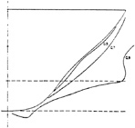


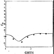

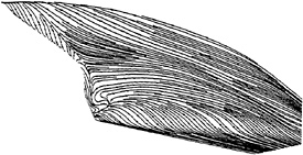
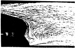


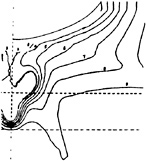


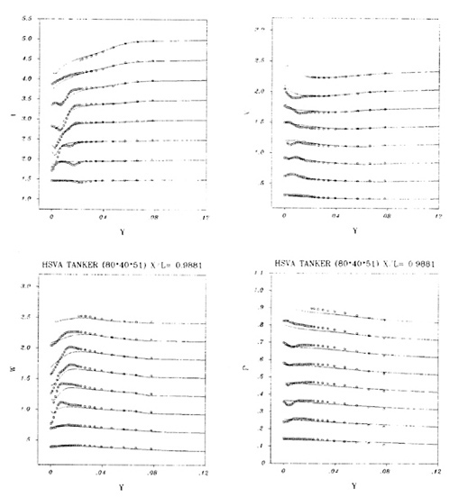
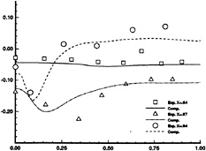
Figure 12- Girth wise Cp distributions- Uni-exponential scheme- Grid II.
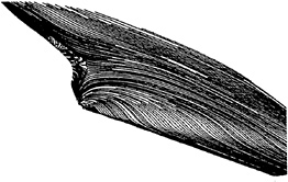
Figure 13- Wall flow- Uni-exponential scheme-Grid II.
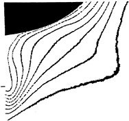
Figure 14- Axial velocity contours- Uni-exponentiel scheme- x/L=0.976-Grid II.
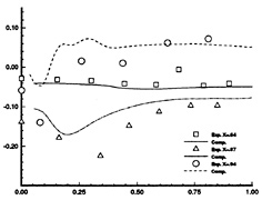
Figure 15- Girthwise Cp distributions- CPI scheme-Grid I.

Figure 16- Wall flow- CPI scheme- Grid I.

Figure 17- Axial velocity contours- CPI scheme-x/L=0.976-Grid I.

Figure 18- Axial velocity contours- Reduction of the turbulence viscosity-x/L=0.976-Grid I.

Figure 19b- W profiles as functions of y, for several depths z=cste, measurements; ---, Standard Uni-exp. computations; — vT modified computations. x/L=0.978-Grid I.

Figure 19a- U profiles as functions of y, for several depths z=cste, measurements; ---, Standard Uni-exp. computations; — vT modified computations. x/L=0.978-Grid I.
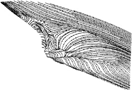
Figure 20- Wall flow- Computations with a reduction of eddy viscosity-Grid I.
DISCUSSION
by Dr. Yoshiaki Kodama, Ship Research Institute, Tokyo, Japan.
The authors conducted a rather definitive work which answers most of the questions raised in the 1990 SSPA Workshop, with respect to the disagreement between the measured and computed wake distributions of the HSVA tanker. I agree with the authors that the turbulence model is mainly responsible for the disagreement. I would, thus, like to ask the authors how can we improve the available turbulence models in order to accurately predict the wake distributions?
Author's Reply
We believe that it is time to implement new turbulence models which are not based on the eddy viscosity concept if the simulation of complex three-dimensional flows is aimed. Encouraging results are already obtained with several full Reynolds stress closures employed to computed three dimensional flows (see [1] & [2] for instance). However, it is now difficult to evaluate the likely numerical difficulties associated with the eviction of turbulent viscosity. We guess that the correct treatment of the turbulent coupling will require severe improvements of the present methodology.
Sotiropoulos, F. and Patel, V.C., “Numerical Calculation of Turbulent Flow through a Circular-to Rectangular Transition Duct Using Advanced Turbulence Closure,” AIAA Paper 93–3030, AIAA 24th Fluid Dynamics Conference ( 1991).
Chen, H.C., “Calculations of Submarine Flows by a Multiblock Reynolds-Averaged Navier-Stokes Method,” Proc. of the 2nd Int. Symp. on Engineering Turbulence Modelling and Measurements ( 1993).
DISCUSSION
by Professor Lars Larsson, FlowTech International and Chalmers University
This is a very interesting and careful study of the flow around one of the test cases of the 1990 SSPA-CTH-IIHR Workshop on Ship Viscous Flow. A new and effective grid is used and grid independence is reasonably well-demonstrated. Different discretization schemes and two standard turbulence models are used. The results seem to verify what was suspected at the Workshop, namely that the results are rather insensitive to variations of this kind. Good results are obtained in all cases for the outer part of the wake, but the central part is wrong.
The drastic improvement in the results caused by the ad hoc change to the eddy viscosity in the vortex is extremely interesting, and the excellent results obtained in this way seem to indicate that it is the turbulence model that has caused the problems everyone has had so far. The reduction in turbulence levels in the thick part of the boundary layer is well-known from experiments and our group tried a more drastic variation already at the Workshop, namely to set vT=0 aft of X/L=0.8. This gave a slight improvement, but not at all as large as in the present paper. However, turbulence data are available for the HSVA tanker (see the paper by Dr. Kux et al. at the Osaka Colloquium in 1985) and it would be very interesting to see whether the present ad hoc modification of the turbulence model is substantiated by that data.
Author's Reply
At this time, we did not make any comparisons with turbulence data since they were not available to us. However, it is planned to make such comparisons for the CFD Workshop devoted to the “Improvement of Hull Forms Design” which will be held in Tokyo in 1994. It will be interesting to check if these ad-hoc modifications of the turbulence model improve also the description of turbulence data.
DISCUSSION
by Steve Watson, Hampshire, DRA
To which method did you apply your viscosity?
Author's Reply
In this paper, the reduction of turbulent viscosity was done for calculations conducted with method I. Since then, the same modification was applied to calculations associated with method II with a similar effect on the near wake.
DISCUSSION
by Prof. A.Y.Odabasi, Technical University of Istanbul, Turkey
I would like to congratulate the authors for an excellent paper and even better presentation. I would like to provide some additional information which may assist in their future work:
-
The measure offered by Prof. M.Tulin, already exists in turbulent shear flow calculations, known as the effects of extra strain rates, largely advocated by Prof. P. Bradshaw of Stanford University (ex-Imperial College, London) and his proposals were published by AGARD.
-
During the PHIVE project, jointly conducted by BSRA and NMS, three models were tested in the large wind tunnel and these measurement included turbulent quantities up to (including) triple velocity correlation terms. Energy balance near vortex cores in the stern region showed that these the dissipation was balanced by diffusion (not by production as is the case near the wall). This feature was brought out in Ref. [16]. Unless transport equations reach to a maturity to model turbulence as measured these anomalies will continue
References:
[16] Odabasi, A.Y., and Davies, M.E., “ Structure of complex turbulent shear flow,” Proc. 3rd Symp. on Numerical and Physical Aspects of Aerodynamic Flows, Long Beach, CA, 1985
Author's Reply
We are aware of many works concerned with curvature effects related to specific configurations. However, we do not know any general approach which could be used in a general purpose computational code to modify the turbulent viscosity in complex three-dimensional flows. Moreover, it is difficult to determine if the reduction of turbulent stresses is mainly due to curvature effects.
DISCUSSION
by Professor M.Tulin, University of California at Santa Barbara
You reported significant improvements in comparisons, when you reduced the Reynolds stress in the longitudinal vortex by a factor of 2.5. In flows with significant streamline curvature the pressure gradients normal to the streamlines can strongly effect the turbulent fluctuations in the normal direction. This is an effect analogous to that due to vertical density gradients in the ocean and the atmosphere; in these cases vertical turbulence can be, and often is strongly suppressed and becomes strongly isotropic. I mention this because there is a large literature on the subject (see Monin's book, for example). I am quite sure that this analogy has already been carried over to homogeneous flows with curved streamlines and applied to flows with vortices, etc. This effect is not part of the Baldwin-Lomax model, but it should be added; this would result in anisotropic Reynolds stresses.
Author's Reply
Thank you for your comments and helpful remarks but we feel that it is not easy to sensitize the turbulent viscosity to the complex streamline curvature that occurs in such a situation.
DISCUSSION
by Dr. A.J.Musker, Defense Research Agency, Haslar, England
A previous Haslar study [1], published in the wake of the 1990 Gothenburg Workshop, indicated that future CFD validation studies should avoid attempts at improving the accuracy of discretization schemes and recommended instead “ (that) a comprehensive assessment of different wall treatments and turbulence models (should be undertaken).” The present study confirms that the solution is insensitive to the numerical scheme but is extremely sensitive to local changes in turbulence diffusivity.
In the most recent Haslar study (presented at this Conference), we cite the presence of the upstream support wire as the possible cause of the “hook” observed in the contours for axial velocity in the propeller plane. Our only evidence for this is the observation that when the
support wire used in the experiment was included (albeit crudely) in the RANS calculation it had the effect of introducing a hook downstream. The only other occasion where a hook was observed, in any of our predictions without the support wire, occurred when the (current) solution was far removed from convergence. If such a solution was then driven more and more towards convergence the hood would eventually vanish. I would be interested to learn whether the present authors have observed similar behavior and whether they are confident that the solution displayed in Figure 18 had truly converged.
Notwithstanding the above cautionary note, the findings in the present paper offer an entirely different, less troublesome, and more exciting explanation for the presence of the hook —namely, that it is associated with a reduced eddy diffusivity within the core of the longitudinal bilge vortex. I say less “troublesome” because our own investigation casts unwanted doubt on the validity of the experiment data which were carefully measured and compiled by the Hamburg team; I say “exciting” because this new finding supplies us with a tantalizing lead which will allow the CFD community to focus attention on the turbulence models with a view to introducing some consistent mechanism for attenuating the eddy diffusivity within such a vortical flow.
The community will want to know which team is right—is the hook caused by the presence of the support wire? Or is it caused by the inherent properties of the turbulent fluid? Time will tell, but I'm bound to say that the case for the former, resting as it does on an imperfect grid, is much weaker in the light of the authors' findings. This paper is an excellent example of what can be achieved by systematic validation studies and I offer the authors my sincere congratulations.
Author's Reply
We agree with Dr. Musker and confirm that it is very important to get a converged solution, although it is almost impossible to reduce the non-linear residuals to machine-zero for this kind of flows. Actually, the evolution of near-wall quantities appears to provide a Unstable sensor of practical convergence for this class of applications, once the non-linear L2-residuals are reduced by 3 to 4 orders of magnitude. The flow resulting from a local reduction of turbulent viscosity obeys these criteria.
Concerning this particular flow, we noticed that an intense unsteady longitudinal vortex appeared if the computations are started in laminar regime. Once the turbulence model is activated, this vortex and the associated hook-shaped structure slowly disappear to give the well-known unsatisfactory results. Then, if we start from this turbulent solution and reduce the turbulent viscosity by an ad-hoc factor in the ad-hoc region, the intensity of the longitudinal vortex grows again, then stabilizes during several hundreds of non-linear iterations, giving birth to the distorted wake pattern and the secondary line of convergence illustrated in this paper.
DISCUSSION
by Dr. Ming Zhu, University of Tokyo
Have you ever seen the flow separation in your computed results? With our numerical study (see our paper in the present conference), we found that the distortional wake pattern in the propeller plane is produced by the flow separation in which phenomenon the Reynolds stress intensity is observed, in many experiment, lower than those in thin turbulent boundary layer. That means that if the flow separation can not be revealed in the numerical simulation, it may be quite difficult to simulate the distortional wake pattern well.
Author's Reply
As indicated in your very interesting paper presented at this conference, the reduction of turbulent shear stresses is due to the conjunction of two phenomena: (i) the thickening of the boundary layer, (ii) the occurrence of a longitudinal flow reversal region near the hub of the hull. However, we guess that the distorted wake pattern observed in the propeller plane is not only due to the presence of this small separated region. Indeed, a small separated region was simulated in our first calculations presented at the Goteborg's Workshop in 1990 but nevertheless, we were not able to capture neither the hook-shaped structure of isowakes nor the longitudinal skin friction convergence line.
Effects of Turbulence Models on Axisymmetric Stern Flows Computed by an Incompressible Viscous Flow Solver
C.H.Sung, J.F.Tsai, T.T.Huang, and W.E.Smith
(David Taylor Model Basin, USA)
ABSTRACT
An incompressible Reynolds-averaged Navier-Stokes (RANS) computational procedure which employs multigrid, multiblock, and local refinement techniques is presented. The effects of grid spacing and grid stretching on the convergence rate of pressure residuals are investigated. In the computation of turbulent flow over an axisymmetric body the grid distributions in the streamwise, azimuthal, and normal-to-the-wall directions and the grid stretching factor normal to the wall are varied. Quantification of computation errors by a solution-to-solution comparison is used to achieve a grid-independent numerical solution. Numerous computations using a three-dimensional computer code with a multigrid capability are then made on four axisymmetric bodies at a Reynolds number (RL) about 107 to investigate the variation of grid distribution requirements at higher RL. The grid distributions are refined to adapt to the local flow conditions on the body. More grid points are needed in regions of rapid pressure variation and finer grid density is required for flow at a higher Reynold number. The total grid cell number is proportional to the square of (RL/y1+) and inversely proportional to the aspect ratio of the first grid cell normal to the wall. A grid independent numerical solution has been obtained from the present RANS computer code when the average value of y1+ is less than 7, and the rate of solution convergence is controlled by avoiding the use of grid cells with an excessively large aspect ratio and extreme grid stretching. Comparisons with experiment are presented for axial velocity and turbulent shear stress profiles in the stern regions of four axisymmetric bodies are used to evaluate and validate various turbulence models. The root-mean-square (RMS) differences of the measured and computed flow variables are given. Two modifications to the Baldwin-Lomax turbulence model are shown to improve the predictions of axisymmetric stern flows.
A brief description is also given of a new numerical approach based on multiblock, multigrid and local refinement techniques that has been implemented in IFLOW. Prediction of three-dimensional complex flows at high Reynolds numbers can be accomplished along with a fine spatial resolution and reduced requirements for computer memory and cpu time.
NOMENCLATURE
|
ax |
=axial-to-normal aspect ratio of the 1st grid cell from the wall |
|
aθ |
=circumferential-to-normal aspect ratio of the 1st grid cell from the wall |
|
A+ |
=26, Eq.(5) |
|
C |
=chord length of hydrofoil |
|
Cτ,Cf |
=local, mean skin friction coefficient |
|
CF(ITTC) |
=the 1957 ITTC friction correlation line |
|
Ccp |
=1.2, Eq.(6) |
|
Ch |
=1.55, δ=Chymax |
|
Ckleb |
=0.65, Eq.(6) |
|
Cβ |
=0.01, Eq.(8) |
|
E |
=preconditioned matrix, Eq.(2) |
|
F,G,H |
=flux vectors in x,y,z directions, Eq.(2) |
|
F(y) |
= |
|
Fwake |
=ymaxFmax |
|
|
|
|
|
|
|
k |
=0.4, von Karman constant, Eq.(5) |
|
K |
=0.0168, Clauser constant |
|
L |
=length of axisymmetric body |
|
l |
=mixing length |
|
N |
=total number of data points or grid cells |
|
MW |
=computer memory in million words |
|
nx,nθ,ny |
=grid cell numbers in axial, circumferential, and normal to the wall directions |
|
|
|
|
BL |
=Baldwin-Lomax turbulence model |
|
q |
=primitive flow variable vector, Eq(2) |
|
|
|
|
Rmax |
=maximum radius of the hull |
|
r |
=radius, ro=hull radius |
|
u,v,w |
=velocity components in x,y,z directions |
|
x,y,z |
=coordinate system |
|
U∞ |
=reference velocity |
|
uτ |
=frictional velocity, |
|
vc |
=computed flow variable |
|
vm |
=measured flow variable |
|
y1 |
=distance from the wall to 1st grid cell center |
|
ymax |
=value of y at the maximum of F(y) |
|
|
|
|
y+ |
=uτy/v, y=distance from the wall |
|
|
|
|
−u′v′ |
=turbulent shear strss |
|
t |
=a parameter in Table 1, 95% confidence limit=t×RMS |
|
α,β |
=preconditioned parameters, α=−1, β=1 |
|
δ |
=boundary layer thickness |
|
ρ |
=mass density of fluid |
|
v |
=kinematic viscosity of fluid |
|
vt |
=eddy viscosity |
|
|
=inner eddy viscosity, Eq.(4, 5) |
|
|
=outer eddy viscosity, Eq.(4, 6) |
|
|
|
|
|
|
|
|
|
|
|
|
|
Δu |
=computed velocity difference at two RL'S |
|
ω |
=vorticity, Eq.(6) |
|
|ω|max |
=maximum value of |ω| |
|
τ |
=wall shear stress |
|
τij |
=Reynolds stress tensor, Eq.(3) |

INTRODUCTION
Recent advances in Computational Fluid Dynamics (CFD) based on numerical solutions of the Reynolds-Averaged Navier-Stokes (RANS) equations have demonstrated a capability to predict the physics of complex flows as measured in model experiments. Computer codes have been developed for hydrodynamic applications where the flows are treated as incompressible and the Reynolds numbers are high (order of 10 6 to 109). However, such codes must be thoroughly validated in order to assess their utility and limitations as design tools. There are many types of errors which the validation process seeks to identify and, hopefully, eliminate. These include numerical errors, physical model errors, and even coding errors. In this paper, a RANS code, IFLOW (Sung and Griffin[1], Sung et. al.[2], and Tsai et. al.[3]) is used as a vehicle to quantify such error sources. The numerical errors associated with grid resolution, grid stretching and convergence rate of the pressure residuals are investigated. Quantification of these errors by solution-to-solution comparison is essential in order to achieve a grid-independent numerical solution. The most critical physical errors are induced by the turbulence model. The errors associated with the turbulence model can only be evaluated after a grid-independent solution is obtained. Performance of the turbulence model can then be assessed by comparisons of measured and computed results. In this paper the measured pressures, skin friction, turbulence shear stress and axial velocity profiles of turbulent axisymmetric stern flows are used to evaluate computed results using various grid resolutions. The RMS differences between the measured and computed flow variables are used to quantitatively assess the validity of the numerical technique.
In the computation of turbulent flow over an axisymmetric body, the grid distributions in the streamwise, circumferential, and normal-to-the-wall directions and the grid stretching in the normal-to-the-wall direction are varied to obtain a grid-independent numerical solution. The distributions and spacings of the flow-adapted grids are successively refined. More grid points are needed in the region of rapid pressure variation and
finer grid density is required for flow at higher Reynolds numbers. The center of the first grid cell normal to the wall (y1) must be set inside the viscous sublayer to obtain a grid-independent solution. This requirement is satisfied by keeping the average value of ![]() less than 7, where uτ is the factional velocity and ν is the kinematic viscosity of the fluid. The rate of solution convergence is monitored during the computation to identify the presence of grid cells with excessively large aspect ratios.
less than 7, where uτ is the factional velocity and ν is the kinematic viscosity of the fluid. The rate of solution convergence is monitored during the computation to identify the presence of grid cells with excessively large aspect ratios.
Computation of body drag at high values of Reynolds number is a major challenge for any CFD code. The effects of grid resolution and turbulence models on the computed total fcitional drag coefficients of the axisymmetric bodies are presented. This demonstrates the status of CFD drag prediction by an incompressible RANS code. An example is also given of RANS computations at two Reynolds numbers to address one aspect of scale effects.
DESCRIPTION OF NUMERICAL METHOD
The three-dimensional, incompressible, Reynolds-averaged Navier-Stokes equations is solved using the artificial compressibility approach first proposed by Chorin [4] and subsequently generalized and improved by Turkel [5,6]. This approach has been successfully used by Chang and Kwak [7], Kwak et al. [8], and many others. The formulation of IFLOW [1,2,3] developed at the David Taylor Model Basin is outlined in the following
Eqt+Fx+Gy+Hz=0,
or
qt+E−1Fx+E−1Gy+E−1Hz=0
(1)
where the subscripts indicate partial derivatives with respect to time t, and the three coordinates x, y, and z. The preconditioned matrix E and the column vectors of the dependent variables q and of the three components of fluxes F, G and H are defined as

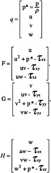
(2)
where p is the pressure, ρ is the constant density, u, v and w are the three Cartesian components of the mean velocity and the Reynolds stresses are defined as
i, j=1, 2, 3 (3)
where u=(u1,u2,u3)=(u,v,w), (x1,x2,x3)= (x,y,z), v is the sum of the kinematic and eddy viscosities, and Rn is the Reynolds number. The variables are nondimensionalized by the free stream condition at infinity in the following manner: u, v and w by U∞; p and τ by ![]() x, y and z by L;
x, y and z by L; ![]() L is the body length; and α and β−2 are the preconditioned parameters. Numerical experiments indicate that the choice of α=−1 and β=1 is adequate.
L is the body length; and α and β−2 are the preconditioned parameters. Numerical experiments indicate that the choice of α=−1 and β=1 is adequate.
The spatial discretization is based on the cell-centered central difference finite-volume formulation. An explicit one-step, five-stage Runge-Kutta time-stepping scheme is used. In this scheme only three evaluations of the artificial dissipation term are made at the first, the third and
the fifth stages with an appropriate weighting at each stage to increase the stability limit. Specifically, the parabolic stability limit along the real axis has been raised to 9 which is advantageous in terms of stability when solving the Navier-Stokes equations. The three techniques used to accelerate the rate of convergence are local time-stepping, implicit residual smoothing and multigridding. The local time step size when defined to include both the convective and the viscous terms has been found to be more stable than that which is estimated by including only the convective term. Three smoothing parameters are used in the residual smoothing technique. These parameters are fixed as constants but are self-adjusting to flow characteristics, and are properly scaled to reduce the undesirable effect arising from high aspect ratios of the grid cells. It is essential to add an appropriate amount of artificial dissipation to suppress spurious oscillations which occur in all central difference schemes. The conventional unidirectional dissipation where the dissipation is proportional only to the maximum eigenvalue of the flux Jacobian in that coordinate direction has been modified to appropriately blend the maximum eigenvalues in all three coordinate directions. Numerical experiments with the revised artificial dissipation terms with carefully devised boundary conditions for the dissipation terms have demonstrated that the revised dissipation models are robust and accurate in the calculation of the flow problems which include high aspect ratio grid cells.
The multigrid method developed by Jameson [9] to accelerate solution convergence has been adopted. By the cyclic use of a sequence of fine to coarse grids, the multigrid technique is very effective in damping the solution modes with long wave lengths which are primarily responsible for slow convergence. Both V- and W-cycle multigrid techniques are used. Boundary conditions are updated at each Runge-Kutta stage of every grid level in the fine-to-coarse path, but they are not updated in the coarse-to-fine path. This practice is mainly used to avoid introducing boundary condition interpolation errors. For ease of coding the grid cell numbers in all the coordinate directions used in a coarse grid is selected to be half of that in the fine grid.
The boundary conditions used on the solid wall are that the three velocities and the normal pressure gradients are all zero. The far field boundary conditions which include both the inflow and the outflow through the boundaries are based on a zero-gradient for the three velocities and a non-reflecting condition for the pressure ; Hedstrom [10], and Rudy and Strikewerda [11]. The non-reflecting boundary condition is particularly important for computation in a relatively small domain and has been carefully implemented.
TURBULENCE MODEL
A simple modification of Baldwin-Lomax turbulence model [12] is used in this paper. The Baldwin-Lomax formulation of eddy viscosity is similar to the algebraic eddy-viscosity model of Cebeci and Smith [13] but is easier to implement in the RANS code. The inner and outer eddy viscosity of the turbulent wall model are defined as
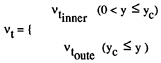
(4)
where y is the normal distance from the wall, and yc is the value of y at which the values of eddy viscosity from the inner and outer formulas are equal.
(5)

(6)
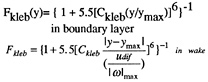
For a wall boundary layer, Fwake=ymaxFmax, and
Fkleb(y)={1+5.5[Ckleb(y/ymax)]6}−1,
where Fmax is the maximum value of ![]() that occurs in a profile and ymax is the corresponding value of y at which it occurs. The Kkleb(y) is the Klebanoff intermittency factor. The constants used are: k=0.4,
that occurs in a profile and ymax is the corresponding value of y at which it occurs. The Kkleb(y) is the Klebanoff intermittency factor. The constants used are: k=0.4, ![]() wall shear stress), Ckleb=0.65, Ccp=1.2, and K= 0.0168=the Clauser constant.
wall shear stress), Ckleb=0.65, Ccp=1.2, and K= 0.0168=the Clauser constant.
In the stern regions of axisymmetric bodies the standard Baldwin-Lomax model overpredicts the values of turbulent shear stresses and streamwise velocities. Two simple modifications to the standard Baldwin-Lomax model are made for these
flows. The modifications are made based on the experimental data of Huang et al. [14,15,16] and are applied only to the values of ![]() as
as
(7)
and
(8)
where
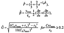 ,
,
and ![]() .
.
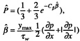
The constants Cβ=0.01 and Ch=1.55(Chymax =δ=the boundary-layer thickness), were obtained by conducting numerical experiments using the measured velocity profiles of Huang et al., and ro is the local radius of the hull. The modified turbulence model used in equations (7) and (8) will be referred to as BL-G, and BL-GP, respectively, and both are simple modifications of the Baldwin-Lomax (BL) model. The letters G indicate the modification is based on the flow geometry of an axisymmetric boundary layer, Eq(7), and GP indicates that the modification is based on the flow geometry and pressure gradient, Eq(8). The modifications apply in the stern region where the axial pressure gradient is positive (adverse).
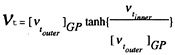
In the symmetric wake of a single axisymmetric body or a two-dimensinal foil the modified eddy viscosity of Renze, Buning, and Rajagopalan [17] is used,
(9)
where
The value of ymax is set at |ω|max and the Klebanoff function is applied outside of ymax. Inside of ymax the eddy viscosity is constant and is set equal to the computed value of ![]() at ymax. The wake becomes asymmetric when the axisymmetric body or foil is at angle of attack. The center line of the asymmetric wake is set at the location of the minimum velocity in the wake. The values of ymax are set at two locations of |ω|max from upper and lower wake. The value of
at ymax. The wake becomes asymmetric when the axisymmetric body or foil is at angle of attack. The center line of the asymmetric wake is set at the location of the minimum velocity in the wake. The values of ymax are set at two locations of |ω|max from upper and lower wake. The value of ![]() takes the maximum value from either side of the wake center line. Inside the two locations of ymax the eddy viscosity is constant and the Klebanoff function is applied outside of ymax.
takes the maximum value from either side of the wake center line. Inside the two locations of ymax the eddy viscosity is constant and the Klebanoff function is applied outside of ymax.
The problem of multiple peaks in the Baldwin-Lomax Fmax function has previously been reported by Degani and Schiff [18]. The modification of the Baldwin-Lomax model made by Degani and Schiff is implemented in the IFLOW code for an axisymmetric body at angle of attack. The differentiation between the vorticity within the attached boundary layers from the vorticity on the surfaces of separated vortices is made to select a length scale based on the thickness of the attached boundary layers rather than one based on the radial distance between the body surface and the surfaces of separated vortices. This modification eliminates the possibility of locating the value of ymax at the surface of the separated vortex and causing an excessively large eddy viscosity.
RESULTS AND DISCUSSION
The comparison of the typical rates of convergence of single grid, 3-level V-cycle multigrid and 3-level W-cycle multigrid based on the calculations on a 96×32×48 grid of a complex appendage-flat plate juncture flow at Rc=6.2×10⁵ is shown in Fig. 1, where Rc in the Reynolds number based on the chord length of the appendage. The residual is defined as the RMS difference between the nondimensional pressures at the (n+1)th and nth cycle, pn+1 and pn,
(10)
where N is the total number of points. As expected, the W-cycle multigrid converges fastest and the single the slowest. The results presented in this paper are for converged residuals of 3×10⁻³ to 10−4 which indicate satisfactorily convergence of the numerical solutions. Around 100 V-cycle multigrid iterations were generally sufficient to achieve the converged numerical solutions with the residuals less than 3×10⁻³.
Computation of the flow field and drag of an axisymmetric body at a high Reynolds number is a major challenge to CFD capability. The effects of grid resolution and turbulence models on the computed flow field and drag coefficients of the axisymmetric Suboff model [16] and the DTNSRC Axisymmetric Body 1, 2 and 5 [14,15] are presented to illustrate the status of the incompressible IFLOW RANS code. The grid-independent solution is defined ideally as the solution of the finite difference equations that approaches the exact solution of the corresponding partial differential (RANS) equations as the grid spacing approaches zero. Since no exact solution of the RANS equations is available for an axisymmetric body at high Reynolds numbers to validate the numerical results, it is necessary to generate numerous numerical solutions for various grid spacings and distributions to compare with experimental measurements. Validation of a RANS computer code can only be made by this tedious numerical-experimental comparison. Quantification of measurement uncertainties are generally available for high-quality experiments. The root-mean-square (RMS) value of the difference between the computed and measured values of the flow variables, respectively defined as vc and vm, is
(11)
where N is the total number of data values used in the comparison. In the presentation of the following results the measurement uncertainties, the RMS differences, and the average values of y1+=uτy/ν for the first grid center normal to the wall are reported for all the computations. The grids are distributed in the axial, circumferential, and radial directions of the axisymmetric body. The distribution of axial grids is selected according to the magnitude of the axial pressure gradient on the body; finer grids are used in the regions of higher pressure gradient. The distribution of circumferential grids is chosen to keep the aspect ratios of grids within the limit that provides good solution convergence (residuals of less than 3 ×10⁻³ in about 100 iteration cycles). The distribution of radial grids, made to resolve the boundary layer characteristics on the hull, requires that y1+ of the first grid center from the wall be limited to less than the thickness of the laminar sublayer. The effects of grid distribution on the computed pressure and skin friction coefficients on the body, the axial velocity and turbulent shear stress profiles at two axial locations of x/L=0.904 and 0.978 on the Suboff Axisymmetric Body have been shown in Reference 3. The computed RMS differences of the flow variables as a function of the average values of y1+ for the Suboff model are shown in Fig. 2. The Reynolds number based on the body length is 1.2×10⁷. As shown in Fig. 2 and the results of Reference 3 when the average value of y1+ of the first grid center from the wall is smaller than 7 every computed viscous flow variable approaches a grid-independent solution. It was found that the computed pressure coefficients approach the grid-independent solution faster than the computed skin friction coefficients.
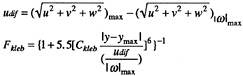
The effect of turbulence model parameters on the computed results can be evaluated after a grid-independent solution has been achieved. An example of the effect of choice of turbulence model parameters on the computed viscous flow variables with a 112×32×64 grid (5.5<y1+<7.9) is shown in Table 1 and Figs. 3 and 4. It is evident that the original Baldwin-Lomax turbulence model must be modified for thick stern boundary layers. The standard Bladwin-Lomax turbulence model was found to overpredict the measured eddy viscosity by as much as a factor of 4, mixing length by a factor of 2, and Reynolds stress by a factor of 2. These discrepancies will generally cause an overprediction of axial velocities in the propeller plane by up to10% of the free stream velocity. The prediction of full-scale ship speed and propulsor rotation speed imposes stringent accuracy requirements for experimental and computational data. Therefore, continued improvement of experimental and computational accuracy is essential to meet CFD validation requirements. The turbulence model we proposed here is an interim rather than a final solution. Critical examination of the measured and computed Reynolds stresses and velocity profiles, as illustrated in this paper is helpful for assessing the validity of turbulence models. Without such a careful examination and detailed comparison, the utility of CFD can be seriously
compromised. Table 1 indicates that the two modified Baldwin-Lomax turbulence models (BL-G, and BL-GP) with the value of the average y1+ smaller than 7, the RMS differences between the computed and measured pressures, skin frictions, axial velocities, and turbulent shear stresses are within the measurement uncertainties. Furthermore, Table 1 shows that the computed total frictional drag coefficients, Cf, are almost equal to or smaller than the value of the standard ship-model correlation line of the 1957 International Towing Tank Conference , CF(ITTC), depending on whether the value of y1+ for the grid used is smaller than or greater than 7. During the course of computation it was noted that grid cells of excessive aspect ratios reduced the rate of convergence. As a result, the circumferential grid number was increased to reduce the aspect ratios and in turn provided an improved rate of convergence. The total pressure drag of the body was also computed and a slight oscillation with increasing grid density was noted. Further improvement of the pressure drag computation has been made by using a local refinement technique to a generate fine grid around the body.
The modified Baldwin-Lomax turbulence model (BL-GP) was used to predict the flow over the Suboff Axisymmetric Body. The results are shown in Figs. 5 and 6 using a grid of 128×32×88. It is seen that satisfactorily computed results for axial velocity and turbulent shear stress profiles were obtained for an average value of y1+=4.4. The computed axial velocity profiles at RL=6.6×10⁶ and 2.5×10⁷, and the computed profiles of the difference in axial velocity at the two RL's for the DTNSRDC Axisymmetric Body 1 are shown Fig. 7. These computed results are useful for propulsor design.
The present comparisons of the computed and measured results provide a guide to estimate the minimum number of grid cells in the streamwise (axial), circumferential, and normal-to-the-wall directions, nx, nθ, and ny. In many applications the RANS solutions, which consistently predict flow variables within the measurement uncertainties of the experimental data, will be accepted as grid-independent solutions for engineering applications. The minimum axial and circumferential grid numbers, nx and nθ, needed to achieve grid-independent RANS solutions of flows over axisymmetric bodies at high Reynolds numbers may be estimated as

(12)
where y1 is the first grid center from the wall, ax and aθ are the average values of the axial and circumferential aspect ratios of the first grid cell from the wall with respect to 2y1, Cf is the mean skin friction coefficient, RL=LU∞/v is the Reynolds number based on body length L and free-stream velocity U∞, y1+=y1+=y1uτ/ν, D is the maximum diameter of the body, and v is the kinematic viscosity. The grid spacings normal to the wall direction are stretched according to a hyperbolic tangent function of two control parameters. The value of ny has been varied from 36 to 88 and the stretching parameters have also been varied to obtain a grid with the smallest allowable value of y1+ that possesses a good rate of solution convergence. The ratios of two adjacent grid spacings, Δn+1/Δn, in each direction are normally limited to 1.2> Δn+1/Δn>0.8. The total number of grid cells becomes
(13)
Here a factor is used to allow for 50% more axial grid cells in the wake. The required computer memory M in units of words may be estimated by assuming that about 50 to 60 (used in the present estimates) 64 bit (8 byte) words of memory are needed for each grid cell. Table 4 of Reference 3, which is generated using the estimates of Equations (12) and (13), provides a guide to select the minimum grid numbers and computer memory required to obtain grid-independent RANS solutions for a range of Reynolds numbers at three typical aspect ratios and at two desired values of y1+. The present computer limitation of about 200 megawords (2 gigawords is possible in the near future) of supercomputer memory for CFD production computations with simple grid distributions precludes the use of y1+=1.0 for RL>107. It is evident that a RANS computer code must possess rapid convergence characteristics for large numbers of grid cells with the largest possible aspect ratios in order to perform computations for RL at about 107 to 108 and must be able to provide consistent
engineering grid-independent solutions for a value of y1+ of about 4.0–6.0. It is very difficult to perform an accurate RANS computation at RL=109 with the memory and speed of the present supercomputers with a simple grid distribution technique and it will be a grand challenge for future CFD efforts for many years to come.
RECENT ADVANCES
The value of y1+ must be smaller than 7 to achieve a grid-independent solution. It is noted from Eqs.12 and 13 that the grid cell number is proportional to the square of Reynolds number for the same values of y1+, nx and nθ. The required large grid cell numbers at full-scale Reynolds numbers are the major diffculty and hence the grand challenge for CFD. One seemingly easy approach is to increase the aspect ratios of the grid cells near the wall and to stretch the grid as much as possible away from the wall. However, excessively large aspect ratio of grid cell near the wall and extreme grid stretching anywhere has been found to degrade numerical stability and to slow solution convergence.
A new numerical approach based on a multiblock, multigrid, local refinement method proposed by Sung[19] has been implemented in IFLOW. The multiblock structure makes grid generation for a complex geometry easier. Multigrid techniques significantly accelerate the rate of convergence. The local refinement method provides high spatial resolution of three-dimensional boundary layer and separated vortical flows at reduced computer memory and cpu time. Two sample three-dimensional flow computations for an appendage/flat plate juncture have been made for RC=6.2×10⁵ [1, 20] and are presented in Figs.8, and 9. Traditional grids of 96×48×48 and 192×96×96 were first used. Then three and four levels of local refinement were applied; the performance of IFLOW on a Cray C90 for these two calculations are shown in Table 2. Memory savings of 70% and 92% and reductions of cpu time by factors of 4.3 and 19 respectively have been achieved with the same spatial resolution in the inner viscous layer. The original values of y1+ of 8.4 and 3.7, respectively were maintained for this evaluation. It is very interesting to note from Table 2 that both computer memory savings and cpu reductions improve with an increasing numbers of grid cells in the computational domain. The required solution resolution in the dominantly viscous flow region (boundary layer, vortex core, or three-dimensional separated zone) dictates the acceptable spacings of grid cells in that region. It is very desirable to be able to reduce grid spacing locally in the critial region without changing the overall grid. The local refinement technique doubles grid numbers in all three directions for every level of refinement. Multiple levels of local grid refinement with moderate grid stretching can be used to provide fine grid spacings near the wall. Thus, the method provides the required fine spatial resolution in the dominantly viscous region which is relatively small. This also avoids the use of excessively large aspect ratios of the grid cells near the wall or large grid numbers. Furthermore, the results of numerical experimentation indicate that the present multigrid local refinement technique can provide effective numerical communications across the interfaces of all levels of grid refinement without numerical instability. This multiblock, multigrid and local refinement method can be used to predict three-dimensional complex flows at high Reynolds numbers with fine spatial resolution in a numbers of critical regions. The details of the numerical method and code validation will be presented in future publications.
CONCLUSION
An incompressible Reynolds-averaged Navier-Stokes computational procedure is presented. Numerous computations are made on four axisymmetric bodies at high values of Reynolds number (between 6.6×10⁶ and 1.2×10⁷) to investigate the effects of grid distribution and turbulence model on computed stern flows. The numerical-experimental comparisons are presented for pressure and skin friction coefficients on the body, and axial and turbulent shear stress profiles at several axial locations in the stern region. The root-mean-square (RMS) differences between the measured and computed flow variables are summarized.
It was found that when the average values of y1+ for the first grid center from the wall was smaller than 7, the RMS differences between all the measured and computed flow variables were within the measurement uncertainties, and the computed total skin friction coefficients were approaching the values of the standard ship-model correlation line of the 1957 International Towing Tank Conference. It was also noted that the grid cells with excessively large aspect ratios near the wall and extreme grid stretching reduced the rate of solution convergence. Therefore, it is important to monitor the rate of solution convergence during computations and avoid the use of grid cells having extreme grid stretching and excessively large aspect ratios.
Two simple interim modifications of the original Baldwin-Lomax turbulence model were made for the stern regions of axisymmetric bodies.
The two modified turbulence models provide better predictions of the stern flows for two axisymmetric bodies.
Preliminary sample computations indicate that a multiblock (for complex geometry), multigrid(for fast solution), local refinement (for efficient use of grid cells) method can be used to compute complex flows at high Reynolds numbers with considerably reduced computer momery and cpu time.
ACKNOWLEDGEMENT
This paper is dedicated to Professor Louis Landweber who inspired and led ship hydrodynamic research for twenty-two years (1932–1954) at the David Taylor Model Basin (DTMB) and continued to consult with many of us at DTMB after he came to the Iowa Institute of Hydaulics Research. In this special Numerical Ship Hydrodynamics Conference we join researchers throughout the world to honor your six-decade career of devoted research and distinguish achievement. Privately we would like to assure our most outsdanding alumnus that the “Landweber ” spirit in Ship Hydrodynamics is alive and well at DTMB. This work was supported by the Office of Naval Research. We are grateful to Mr. James A.Fein of ONR for his support. The majority of the work was completed when Dr. J.F.Tsai was a visiting researcher at the Johns Hopkins University from the National Taiwan University during the school year 1991–1992. The NAS program at NASA-Ames Research Center provided their CRAY-2 and CRAY-YMP computer resources for this work.
REFERENCES
1. Sung, C.-H., and Griffin, M.J., “ Improvement in Incompressible Turbulent Horseshoe Vortex Juncture Flow Calculations,” AIAA Paper 91–0022, AIAA 29th Aerospace Sciences Meeting, Reno, Nevada, January 7–10, 1991.
2. Sung, C.-H., Griffin, M.J., and Coleman, R.M., “Numerical Evalution of Vortex Flow Control Devices,” AIAA paper 91–1825, AIAA 22nd Fluid Dynamics, Plasma Dynamics & Laser Conference, Honolulu, Hawaii, June 24–26, 1991.
3. Tsai, J.F., Sung, C.H., Griffin, M.J., and Huang, T.T.,” Effects of Grid Resolution on Axisymmetric Stern Flows Computed by an Incompressible Viscous Flow Solver,” paper presented at the ASME Summer Fluids Engineering Conference, FED-Vol. 158, pp99– 108, June 20–24, 1993.
4. Chorin, A.J.,” A Numerical Method for Solving Incompressible Viscous Flow Problems, ” J. Comp. Phys., vol. 2, pp. 12–26, 1967.
5. Turkel, E., “Preconditioned Methods for Solving Incompressible and Low Speed Compressible Equations,” NASA ICASE Report 86–14, 1989.
6. Tuekel, E., “Review of Preconditioning Methods for Fluid Dynamics,” NASA ICASE Report 92–47, 1992.
7. Chang, J.L.C., and Kwak, D.,” On the Method of Pseudo Compressibility for Numerically Solving Incompressible Flows,” AIAA Paper-0252, 1984.
8. Kwak, D., Chang, J.L.C., Shanks, S. P., and Chakravarthy, S.,” A Three-Dimensional Incompressible Navier-Stockes Flow Solver Using Primitive Variables,” AIAA J., vol. 24, no. 3, pp390–396, 1986.
9. Jameson, A., “Multigrid Algorithms for Compressible Flow Calculation,” in Multigrid Methods II. Lecture Notes in Mathematics series, no.1228, Hackbusch, W., and Trottenberg, U. Eds., Spring-Verlag, New York, 1986.
10. Hedstrom, G.W., “Nonreflecting Boundary Conditions for Nonlinear Hyperbolic System, ” J. Computational Physics. vol. 30, pp222–237, 1979.
11. Rudy, D.H., and Strikewerda, J.C., “ Boundary Conditions for Subsonic Compressible Navier-Stokes Equations, ” Computers and Fluids, vol.9, pp327–338, 1981.
12. Baldwin, B.S., and Lomax, H., “Thin Layer Approximation and Algebraic Model for Separated Turbulent Flows,” AIAA paper 78–257, AIAA 16th Aerospace Sciences Meeting, Huntsville, Alabama, January 16–18, 1978.
13. Cebeci, T. and Smith, A.M.O., Analysis of Turbulent Boundary Layers, Academic, New York, 1974.
14. Huang, T.T., Santelli, N., Belt, G., “ Stern Boundary-Layer Flow on Axisymmetric Bodies,” Paper presented at the 12th Symposium on Naval Hydrodynamics, Wash. D.C., June 5–9, 1978, National Academy of Sciences Wash. D.C., pp 127–157, 1978.
15. Huang, T.T., Groves, N.C., and Belt, G.S., “Boundary Layer Flow on an Axisymmetric Body with an Inflected Stern, ” DTNSRDC Report 80/064, 1980.
16. Huang, T.T., Liu, H.-L., Groves, N. C., Forlini, T.J., Blanton, J.N., and Gowing, S.,” Measurements of Flows Over an Axisymmetric Body with Various Appendages ( DARPA SUBOFF Experiments)” Paper presented at the 19th Symposium on Naval Hydrodynamics, Seoul, Korea, August 24–28, 1992.
17. Renze, K.J., Buning, P.G., and Rajagopalan, R.G.,” A Comparative Study of Turbulence Models for Overset Grids, AIAA paper
92–0437, AIAA 30th Aerospace Sciences Meeting, Reno, Nevada, Jan. 6–9, 1992.
18. Degani, D., and Schiff, L.B.,” Computation of Turbulent Supersonic Flows around Pointed Bodies Having Crossflow Separation,” J. Comp. Phys., Vol. 66, pp173– 196, 1986.
19. Sung, C.H.,” A Multiblock Multigrid Local Refinement Method for Incompressible Reynolds-averaged Navier-Stokes Equations”, 6th Copper Mountain Conference on Multigrid Methods, Copper Mountain, Colorado, April 4–9, 1993.
20. Devenport, W.J., Dewitz, M.B., Agarwal, N.K., Simpson, R.L., and Poddar, K.,” Effects on the Flow Past a Wing Body Junction,” AIAA 2nd Tuebulent Shear Flow Control Conference, Tucson, Arizona, March, 1989.

FIGURE 1. TYPICAL RATE OF CONVERGENCE WITH AND WITHOUT MULTIGRID FOR 96×32×48 GRID

FIGURE 2. RMS DIFFERENCES BETWEEN MEASURED AND COMPUTED FLOW VARIABLES AT VARIOUS VALUES OF y1+

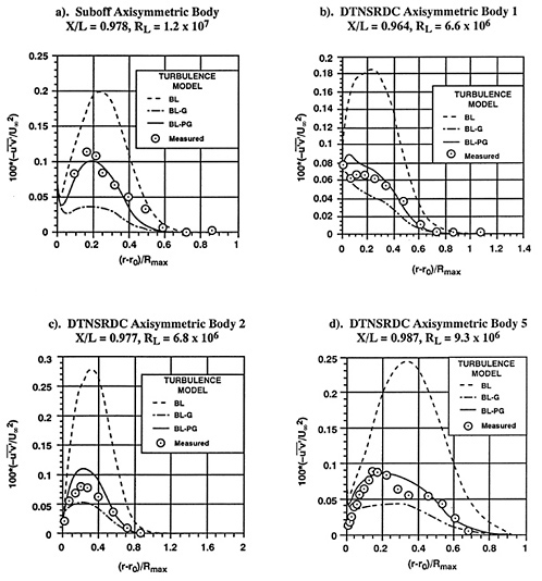


TABLE 1. EFFECT OF TURBULENCE MODELS ON THE RMS DIFFERENCES BETWEEN MEASURED AND COMPUTED FLOW VARIABLES Grid 112×32×64
|
a) Suboff Axisymmetric Body, RL=1.2×10⁷ |
||||||||||||
|
u/U∞ |
|
Cp |
Cτ×104 |
Cf×103 |
y+ave |
|||||||
|
Measurement Uncertainty |
±0.025 |
±0.01 |
± 0.015 |
±2.0 |
||||||||
|
X/L |
0.904 |
0.927 |
0.956 |
0.978 |
0.904 |
0.927 |
0.956 |
0.978 |
||||
|
No. of Points |
19 |
14 |
12 |
16 |
19 |
14 |
12 |
16 |
21 |
17 |
||
|
t |
2.093 |
2.145 |
2.179 |
2.120 |
2.093 |
2.145 |
2.179 |
2.120 |
2.080 |
2.110 |
||
|
BL |
0.050 |
0.013 |
0.007 |
0.049 |
0.089 |
0.111 |
0.131 |
0.116 |
0.023 |
3.0 |
2.778 |
7.658 |
|
BL-G |
0.032 |
0.015 |
0.006 |
0.024 |
0.054 |
0.057 |
0.035 |
0.076 |
0.020 |
2.6 |
2.772 |
7.570 |
|
BL-PG |
0.032 |
0.010 |
0.005 |
0.030 |
0.011 |
0.006 |
0.007 |
0.008 |
0.019 |
2.5 |
2.766 |
7.265 |
|
CF(ITTC): 2.907×10⁻³ |
||||||||||||
|
b) DTNSRDC Axisymmetric Body 1, RL=6.6×10⁶ |
||||||||||||
|
u/U∞ |
|
Cp |
Cτ×104 |
Cf×103 |
y+ave |
|||||||
|
Measurement Uncertainty |
±0.025 |
±0.01 |
±0.015 |
±2.0 |
||||||||
|
X/L |
0.755 |
0.934 |
0.964 |
0.978 |
0.755 |
0.934 |
0.964 |
|||||
|
No. of Points |
15 |
14 |
16 |
35 |
12 |
9 |
11 |
11 |
9 |
|||
|
t |
2.131 |
2.145 |
2.120 |
2.000 |
2.179 |
2.262 |
2.201 |
2.201 |
2.262 |
|||
|
BL |
0.021 |
0.017 |
0.043 |
0.039 |
0.018 |
0.062 |
0.077 |
0.009 |
0.9 |
2.936 |
7.93 |
|
|
BL-G |
0.021 |
0.011 |
0.028 |
0.014 |
0.019 |
0.021 |
0.019 |
0.010 |
1.2 |
2.919 |
7.78 |
|
|
BL-PG |
0.021 |
0.006 |
0.020 |
0.010 |
0.023 |
0.009 |
0.010 |
0.012 |
1.0 |
2.879 |
7.78 |
|
|
CF(ITTC): 3.229×10⁻³ |
||||||||||||
|
c) DTNSRDC Axisymmetric Body 2, RL=6.8×10⁶ |
||||||||||||
|
u/U∞ |
|
Cp |
Cτ×104 |
Cf×103 |
y+ave |
|||||||
|
Measurement Uncertainty |
±0.025 |
±0.01 |
±0.015 |
±2.0 |
||||||||
|
X/L |
0.840 |
0.934 |
0.970 |
0.977 |
0.840 |
0.934 |
0.970 |
0.977 |
||||
|
No. of Points |
11 |
17 |
14 |
13 |
6 |
14 |
10 |
9 |
12 |
11 |
||
|
t |
2.201 |
2.110 |
2.145 |
2.160 |
2.306 |
2.145 |
2.228 |
2.262 |
2.179 |
2.110 |
||
|
BL |
0.025 |
0.028 |
0.064 |
0.033 |
0.022 |
0.064 |
0.113 |
0.115 |
0.017 |
2.1 |
3.217 |
5.50 |
|
BL-G |
0.014 |
0.042 |
0.026 |
0.018 |
0.016 |
0.008 |
0.019 |
0.017 |
0.020 |
2.0 |
3.211 |
5.51 |
|
BL-GP |
0.025 |
0.027 |
0.037 |
0.019 |
0.026 |
0.014 |
0.016 |
0.019 |
0.015 |
1.5 |
3.157 |
5.35 |
|
CF(ITTC): 3.212×10⁻³ |
||||||||||||
|
d) DTNSRDC Axisymmetric Body 5, RL=9.3×10⁶ |
||||||||||||
|
u/U∞ |
|
Cp |
Cτ×104 |
Cf×103 |
y+ave |
|||||||
|
Measurement Uncertainty |
± 0.025 |
±0.01 |
± 0.015 |
±2.0 |
||||||||
|
X/L |
0.704 |
0.831 |
0.951 |
0.987 |
0.704 |
0.831 |
0.951 |
0.987 |
||||
|
No. of Points |
21 |
18 |
26 |
27 |
21 |
9 |
13 |
17 |
15 |
14 |
||
|
t |
2.080 |
2.101 |
2.056 |
2.052 |
2.080 |
2.262 |
2.160 |
2.110 |
2.131 |
2.145 |
||
|
BL |
0.019 |
0.016 |
0.061 |
0.058 |
0.008 |
0.009 |
0.160 |
0.094 |
0.025 |
3.76 |
2.993 |
5.98 |
|
BL-G |
0.018 |
0.016 |
0.025 |
0.013 |
0.008 |
0.010 |
0.024 |
0.026 |
0.023 |
2.75 |
2.978 |
5.89 |
|
BL-GP |
0.019 |
0.015 |
0.023 |
0.015 |
0.008 |
0.007 |
0.027 |
0.018 |
0.019 |
2.23 |
2.926 |
5.87 |
|
CF(ITTC): 3.038×10⁻³ |
||||||||||||
TABLE 2. MULTIBLOCK MULTIGRID LOCAL REFINEMENT COMPUTATION OF TURBULENT APPENDAGE/FLAT PLATE JUNCTURE FLOW ON CRAY C90 COMPUTER, RC=6.2×10⁵
|
Sample Computation 1. 3-Level Local Refinement to Obtain Resolution of 96×48×48 Grid, y1+=8.4 |
|||||
|
MULTIGRID |
GRID CELLS |
MEMORY (MW) |
CPU(SEC)/ 100 CYCLES |
% SAVING MW |
RED. IN CPU TIME |
|
Without Local Refinement |
221,184 |
11.5 |
430 |
– |
– |
|
With Local Refinement |
49,536 |
3.4 |
99 |
70% |
4.3 |
|
Sample Computation 2. 4-Level Local Refinement to Obtain Resolution of 192×96×96 Grid, y1+=3.7 |
|||||
|
MULTIGRID |
GRID CELLS |
MEMORY (MW) |
CPU(SEC)/ 100 CYCLES |
% SAVING MW |
RED. IN CPU TIME |
|
Without Local Refinement |
1,769,472 |
80.0 |
3600 |
– |
– |
|
With Local Refinement |
71,808 |
6.16 |
191 |
92% |
19 |
DISCUSSION
by Professor V.C.Patel, University of Iowa
I have some questions that could be addressed also to authors of some previous papers in which the Baldwin-Lomax model is used with the first grid point at y+around 7 to 10. The questions are:
“Are these the maximum or minimum, or just average values? How do you determine Cf, the friction coefficient? Do you simply use the slope at the wall? Do you make a correction for the pressure gradients, both longitudinal and transverse? If not, how accurate are Cf and related quantities?”
Author's Reply
In our paper the value of y1+at the first grid point around 7 to 10 is meant to say that the maximum value of y1+ is 10 and the arithmetic mean value is 7. When one value of y1+ is given that is the arithmetic mean value of y1+ for all the grid cells on the body.
The local skin-friction coefficient Cf is calculated by
where the value of ![]() is computed at the cell center of the first grid from the wall when the value of y1+ is less than 7. It is noted that the exact value
is computed at the cell center of the first grid from the wall when the value of y1+ is less than 7. It is noted that the exact value ![]() at the wall must be used when the value of y1+is larger than 7, and can be obtained by extrapolating from the velocities parallel to the wall u(y1) and u(y2) of the first second grid centers at distances y1 and y2 normal to the wall,
at the wall must be used when the value of y1+is larger than 7, and can be obtained by extrapolating from the velocities parallel to the wall u(y1) and u(y2) of the first second grid centers at distances y1 and y2 normal to the wall,
where u(y0) is set equal to 0 at the smooth wall y0 without drag reduction.
No correction for the pressure gradients was made in computing Cf, but the effect due to the streamwise pressure gradient is added to the Baldwin-Lomax model. The total skin-friction was integrated from the local skin-friction. The accuracy of the computed local and total skin-friction coefficients is shown in Table 1.


