
CHAPTER 14
NITROGEN OXIDE EMISSIONS AND THEIR DISTRIBUTORS
INTRODUCTION
Nitrogen Compounds
Nitrogen, the most abundant gas in the atmosphere, is found in a variety of gaseous and particulate forms. The overwhelming amount in air (79 percent of air by volume or 4.6×10¹² tons) is present as relatively inert nitrogen gas, N2. However, the oxidation of nitrogen by bacteria, lightning, organic protein decay, and high temperature combustion and chemical processing causes the appearance of nitrogen in a variety of compounds. The most important, because of health effects and reactivity, are: NO (nitric oxide), NO2 (nitrogen dioxide), NH3 (ammonia) and to a lesser extent N2O (nitrous oxide).
Nitrous Oxide (N2O)
Nitrous oxide, a colorless and odorless gas, has been used as an anesthetic (laughing gas). It is present in the atmosphere in concentrations averaging about 0.25 ppm (Junge 1963, Bates and Hays 1967). There are no direct pollutant sources of N2O, although it may be an indirect and minor product of NO2 photolysis with sunlight and hydrocarbons. The in-
terest in N2O is not in the troposphere (ground level to 8–15 km) where it is practically inert but in photodissociation reactions in the stratosphere. Bates and Hays (1967) indicate that the dissociation of N2O into NO and atomic nitrogen accounts for about 20 percent of the dissociation in the stratosphere. The NO thus formed provides an important sink reaction for ozone.
Ammonia (NH3)
As an industrial emission, ammonia is produced mainly from coal and oil combustion but natural production from biological generation over land and ocean is many times greater than that from anthropogenic sources (250 to 1). NH3’s importance is the significant role it plays in atmospheric reactions in both the nitrogen and sulfur cycles. Nearly three-fourths of the NH3 is converted to ammonium ion condens ed in droplets or particles. These aerosols are then subject to the physical removal mechan isms of coagulation, washout, rainout and dry deposition.
In general, ambient background concentrations of NH3 vary directly with the intensity of biological activity. The highest concentrations occur in the summer and in the tropical latitudes. Concentrations, as reported by many investigators, range from 1 to 10 ppb (Strauss 1972).
Nitric Oxide-Nitrogen Dioxide
NO, a colorless, odorless gas, is formed naturally from the nitrates in various materials by bacteria and then is oxidized to NO2 (Peterson 1956).
Altschuller (1958) and others have reported very hazardous conditions for farm workers near closed silos where NO→NO2 bacterial production has resulted in toxic concentrations of several hundred ppm of NO2.
Organic nitrogen compounds are found in
coal and oil in concentrations of a few tenths to a few percent by weight. Bituminous coal contains 1–2 percent nitrogen, and United States crude oil approximately 0.05–0.5 percent nitrogen (Demski et al. 1973).
Natural gas, while containing up to 4 percent nitrogen gas, does not contain any significant organic nitrogen (Perry et al. 1963). Because organic nitrogen compounds have relatively high molecular weights, they tend to be concentrated in the residual and heavy oil fractions during distillation.
Nitrogen oxides are produced during combustion by the oxidation of organic nitrogen compounds in fossil fuels and by the thermal fixation of atmospheric nitrogen gas, N2.
The primary sources of NO and NO2 as pollutants are combustion processes in which temperatures are high enough to fix N in the air and fuel, and in which the quenching of combustion is rapid enough to reduce decomposition back to N2 and O2. The predominant product of this high temperature combustion is NO. During combustion, approximately 5–40 percent of the nitrogen in coal, and 20 to 100 percent of the nitrogen in oil is oxidized to nitrogen oxides (see Chapter 15).
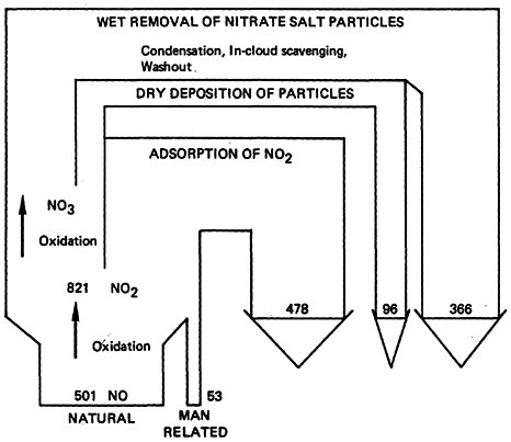
NO is subsequently oxidized to NO2 either in the stack gas or, to a lesser extent, in the diluted plume. Once the NO has been diluted to 1 ppm (1230 μg/m3) or less, the direct reactions with O2 do not contribute significantly to NO2 formation (USEPA 1971). However, the reaction of NO with tropospheric ambient concentrations of O3 (ozone) to form NO2 is rapid. It is believed that the almost everpresent background concentrations of O3 will yield NO2 predominance over NO, although some researchers have reported higher NO than NO2 concentrations in remote areas (Lodge and Pate 1960, Ripperton et al. 1970).
NO2 is removed from the atmosphere either by further O3 oxidation to a nitrous salt or by the more favored conversion to HNO3 in the presence of water vapor. The HNO3 is then rapidly removed by reactions with NH3 and absorption by hygroscopic particles (Strauss 1972)
Nitrogen Oxides
Global Emissions
To estimate the total annual emission of oxides of nitrogen (NOx), emission factors have been applied to the fuel usage of several sources (Robinson and Robbins 1968). According to Robinson and Robbins, the annual production in 1967 was about 53×106 tons with coal combustion contributing the majority, 51 percent, followed by petroleum production and combustion contributing 41 percent. Natural gas combustion on a world-wide basis is comparatively less important (4 percent). However, it should be noted that on a local or regional basis, it could be the major source of NOx. (It should also be noted that these figures include combustion sources only since careful surveys of industrial process losses had not been undertaken at the time these estimates were prepared.) See Table 14–1.
National Emissions
Anthropogenic sources in the United States produce nearly 50 percent of the world’s NOx emissions (USEPA 1971). While emissions from human activities amount to far less than the estimated 50×107 tons of NOx emitted annually from natural sources (USEPA 1971), the spatial concentration of emissions in urban areas leads to concentrations of NOx 10 to 100 times higher than those in non-urban atmospheres.
Fuel combustion is the major cause of anth ropogenic NOx emissions in the United States (See Figure 14–12). In 1972, coal, oil, natural gas and motor-vehicle fuel combustion contributed over 86 percent of the estimated 24.6 million tons of NOx emitted in the United States. Stationary area and point sources account for approximately 64 percent of all the NOx. Direct stationary fuel combustion is the largest source
TABLE 14–1
World-Wide Urban Emissions of Nitrogen Dioxide
|
Fuel |
Source |
NO2 Emissions (106 Tons) |
% Total |
Sub % |
|
TOTAL |
|
52.9 |
100 |
|
|
COAL |
51 |
100 |
||
|
|
Power Generation |
12.2 |
23 |
47 |
|
Industrial |
13.7 |
26 |
52 |
|
|
Domestic/Commercial |
1.0 |
2 |
3 |
|
|
PETROLEUM |
41 |
100 |
||
|
|
Refinery Production |
0.7 |
1 |
3 |
|
Gasoline |
7.5 |
14 |
34 |
|
|
Kerosene |
1.3 |
2 |
6 |
|
|
Fuel Oil |
3.6 |
7 |
16 |
|
|
Residual Oil |
9.2 |
17 |
41 |
|
|
NATURAL GAS |
4 |
100 |
||
|
|
Power Generation |
0.6 |
1 |
25 |
|
Industrial |
1.1 |
2 |
50 |
|
|
Domestic/Commercial |
0.4 |
<1 |
25 |
|
|
OTHER |
||||
|
|
Incineration |
0.5 |
<1 |
|
|
Wood |
0.3 |
<1 |
||
|
Forest Fires |
0.5 |
1 |
||
|
Source: Modified from Robinson and Robbins (1968). |
||||
category (49.7 percent) with coal as the single largest contributor of NOx in this group.
Gasoline powered vehicles are the overwhelming source of transportation-related NOx contributing 32 percent of all NOx and 82 percent of the transportation NOx.
Significant quantities of NOx are emitted from industrial processes, primarily the manufacturing and use of nitric acid and refining of petroleum. On a local scale, electroplating, engraving, welding, and metal cleaning are responsible for industrial NOx emissions which may also be significant. In 1972, industrial process losses accounted for 2.9 million tons of NOx, or 11.7 percent of total nationwide emissions.
Overall, about 77 percent of the total NOx emissions occur in highly populated areas. Eighty percent of stationary source emissions occur in populated areas as do 71 percent of motor vehicle emissions.
The 1972 NOx emissions for the Nation will be defined in greater detail in the following section.
There has been a steady growth of NOx nationwide emissions. The decade of the sixties witnessed a greater increase in emissions than the previous two decades (see Table 14–2).
TABLE 14–2
NITROGEN OXIDES: Estimated Total Nationwide Emissions (106 tons) (USEPA 1974)
|
1940 |
1950 |
1960 |
1970 |
|
6.5 |
8.8 |
11.4 |
22.1 |
Over the past three decades, total nationwide emissions are estimated to have quadrupled. During this period, emissions from motor vehicles have increased at a steady rate of 4.6 to 4.9 percent per year. Emissions from stationary sources, however, have contributed progressively increasing proportions. Total NOx
emissions from power plants have increased at an annual rate of 6.9 to 7.4 percent.
Nitrogen Oxide Concentrations
Controversy and uncertainty about NOx measurement methods have made reliable urban NO and NO2 concentration data almost as scarce as the remote area data. Global remote measurements show NO2 variations with growing season, latitude, and altitude. Lodge and Pate (1966) reported average dry season values of 0.9 ppb and wet season values at 3.6 ppb NO2 in Panama. Junge reported in 1966 measured NO2 concentrations averaging 0.9 ppb in Florida and 1.3 ppb at 10,000 foot high Mauna Kea, Hawaii (Junge 1956). In the continental U.S., several investigators found NO2 values in the 4 ppb range and NO concentrations about 50 percent lower at 2 ppb (Hamilton et al. 1968, Ripperton et al. 1970).
Based upon the estimated global background levels and the annual emissions rates, the average residence time of NO2 in the atmosphere is about 3 days and that of NO is about 4 days. Residence times of atmospheric pollutants reflect the action of natural scavenging processes including photochemical reactions. Figure 14–1 provides a flow diagram summary of the atmospheric NO-NO2 cycle.
The spatial and temporal variations in ambient NO2 concentrations are great. Not surprisingly, the highest concentrations are found in urban regions. Measurements of NO2 have been taken since 1961 through the CAMP and SCAN programs of EPA (formerly NAPCA). However, there is now considerable uncertainty regarding ambient levels and trends for NOx. Although an EPA study of CAMP data for 5 cities reported slight increases in ambient NOx for 1962–1971, the data were obtained by the Jacobs-Hochheiser method for NOx analysis, which has been shown to overestimate ambient NOx levels at low concentrations (CEQ 1975). Thus, these NOx data must be viewed with caution. (See Appendix 14-B)
The National Air Surveillance Network (NASN) program for measuring NOx by a modified Jacobs-Hochheiser method was started in 1972 and it will be several years before the program can provide useful trend data on ambient NOx levels.
EPA has suspended all Air Quality Control Regions priority classifications based on NOx. However, regions where the standards for NO2 are believed to be exceeded are Los Angeles, Chicago, and Baltimore, and possible, New York-New Jersey-Connecticut, Salt Lake City, and Denver.
In spite of the uncertainties in the absolute values, there are NOx data available to indicate the general yearly trends in a few areas. The trends in CAMP observations of nitrogen dioxide are provided in Table 14–3. With the exception of Chicago, annual avenge nitric oxide concentrations of the period 1967–1971 are consistently higher than those of the period 1962–1966.
Annual nitrogen dioxide (NO2) averages show a greater variability among cities than do the nitric oxide averages, and the trends for nitrogen dioxide do not parallel those of nitric oxide. It is not clear whether this deviation is a result of instrument variation, or whether it can be attributed to differences in atmospheric conversion rates in various cities (NAS 1974).
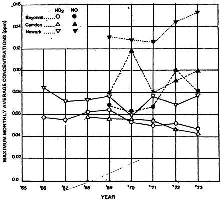
Monitoring data for NO and NO2 in New Jersey cities presented in Figure 14–2 suggest that a pattern of change similar to that observed in the CAMP cities has occurred at these locations. Maximum monthly averages of nitric oxide appear to have increased after 1971, while the levels of NO2 have remained essentially constant over the same period.
In Los Angeles County there has been a direct relationship between increasing NOx emissions and the reported annual average one hour concentrations of NO2. Between 1965 and 1972, NOx emissions have increased in L.A. County at an annual average rate of 3.8 percent per year. The annual average of the maximum hourly average total NOx concentrations has increased approximately 3.2 percent per year from 1965 to
TABLE 14–3
Nitrogen Dioxide Trends in CAMP Cities 1962–71 (National Academy of Sciences 1974)
|
|
Average NO concentration, ppm |
Average NO2 concentration, ppm |
||
|
Station |
1962–66 |
1967–71 |
1962–66 |
1967–71 |
|
Chicago |
0.10 |
0.10 |
0.04 |
0.05 |
|
Cincinnati |
0.03 |
0.04 |
0.03 |
0.03 |
|
Denver |
0.03 |
0.04 |
0.04 |
0.04 |
|
Philadelphia |
0.04 |
0.53* |
0.04 |
0.04 |
|
St. Louis |
0.03 |
0.04 |
0.03 |
0.03 |
|
*The unusually high NO concentration for Philadelphia in 1967–71 is discussed in the section of this chapter on U.S. Nitrogen Oxide Emissions. |
||||
1972 at Burbank and downtown L.A. However, Anaheim and Azusa experienced increases in these annual averages of close to 11 percent per year.
There is more detailed discussion of NOx, hydrocarbon, and oxidant trends and relationships presented in Vol. 3, “The Relationship of Emissions to Ambient Air Quality” of the National Academy of Sciences Report, Air Quality and Automobile Emission Control, September 1974.
Diurnal Nitrogen Oxide Concentrations
The concentrations of NO and NOx in the ambient air change during a typical day. While all aspects of the typical diurnal cycle are not completely understood (Comm. of Mass, 1973, 1974; Coffey and Stasink 1975), it is possible to trace the concentrations of NO and NO2 throughout the day.
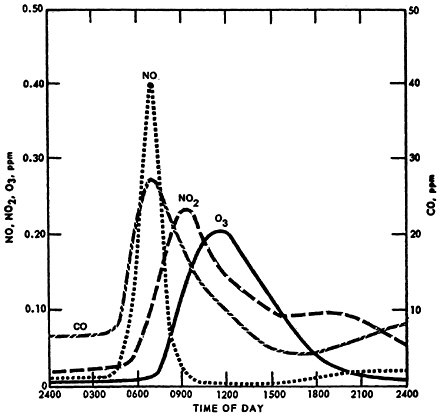
On a normal day in a city, ambient NOx levels follow a regular pattern with the sun and traffic. Nocturnal levels of NO and NO2 are relatively stable and are usually higher than the minimum daily values. During the dawn hours of 6 to 8 a.m., NO begins to increase as a result of automobile emissions. With increasing ultraviolet sunlight to drive the conversion reactions, NO2 concentrations increase until most of the NO is converted to secondary NO2. Photochemical oxidants accumulate as NO decreases to low levels (<0.1 ppm) and they reach a peak about midday. Secondary and tertiary reactions involving NO and NO2 occur leading to complex formations of eye irritants such as PAN (peroxyacylnitrates).
Later in the afternoon, there is decreased mixing, and increased atmospheric stability. Evening rush hour traffic (4 to 7 p.m.) produces another build-up of NO which is not readily converted to NO2 or more oxidants. The absence of sunlight does not completely halt NO2 formation, however. The principal oxidant present, ozone (O3), continues to react rapidly with NO to form NO2, until the O3 supply is
exhausted, and thus the early evening NO2 concentration may continue to rise. This condition may be ascribed to meteorological factors and, on cold evenings, to increased emissions from stationary sources.
A smoothed concentration profile for NO, NO2, carbon monoxide (CO), and O3 in Los Angeles on July 19, 1965, is displayed in Figure 14–3. The figure shows concentration on only a single day but it graphically displays the diurnal phenomenon described above. The NO2 peak lags the NO peak. The build-up of O3 is coincidental with the decrease of NO. The evening increase of NO2 apparently did not occur on this day.
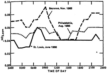
The classical diurnal trend is also apparent in Figure 14–4, which illustrates the diurnal variation in monthly mean 1-hour average NO2 concentrations from St. Louis, Philadelphia, and Bayonne, N.J.
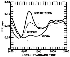
Figure 14–5 compares the diurnal patterns of NO for weekend days and weekdays (for Chicago CAMP stations). The Sunday 8 a.m. peak is about one-third of the weekday peak concentration. On some weekends, some locations have peak values, but these occur between 9 and 11 a.m.
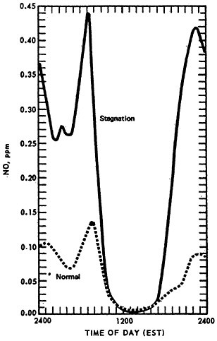
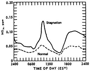
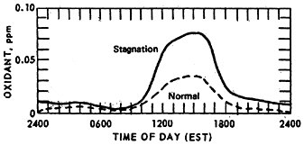
The effect of stagnation conditions on the nitrogen oxide- photo-oxidant relationship is graphically exemplified in the diurnal concentrations of NO, NO2 and oxidants during a stagnating air mass over Washington, D.C. (USDOC 1967). Figures 14–6 through 14–8 compare the diurnal concentration pattern for NO, NO2 and oxidants that occurred during a four day stagnation in Washington, D.C., October 15 to 19, 1963, with a composite of the normal concentrations without stagnation and inversions. The efficiency of the NO-NO2 conversion to photo-oxidants is obvious. During midday when solar energy is most intense, the photo-oxidation of NO and NO2 in the presence of hydrocarbons is so efficient that their concentrations differ little from the norm. Details of these photochemical reactions are discussed in Appendix 14-A.
Seasonal Patterns
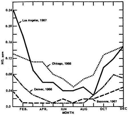
The concentration of NO displays a seasonal variation while that of NO2 does not. For NO, higher mean values are observed during late fall and winter months coinciding with decreased atmospheric mixing and generally less untraviolet energy available for the formation secondary products.
Figure 14–9 shows the seasonal patterns in NO by presenting the mean values by month of the year. The higher winter levels are quite distinctive.
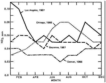
The seasonal pattern for NO2 is less consistent, as seen in Figure 14–10. Thus there appears to be little monthly variation for Denver (1966) and Bayonne, N.J. (1967). Even though a greater amount of NO is converted to NO2 during the summer months, the actual concentrations of NO2 are governed by the rate of conversion to oxidant. This can lead to apparently contradictory comparisons between Los Angeles and Chicago monthly trends.
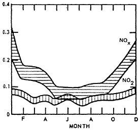
NO2 is highest during summer months in Chicago and during winter months in L.A. On closer examination of the L.A. aerometric data, one finds an inverse relationship between oxidant levels and NO2 levels. The presence of oxidants during summer months, when the synoptic weather condition superimposes a persistent inversion lid over the L.A. basin, and when there is higher solar radiation intensity and higher temperature, effectively scavenges the NO molecules. Figure 14–11.
Indoor Concentrations of Nitrogen Oxides
There is now a very active interest in determining pollutant levels in the home environment. However, very little of the research performed to date has been concerned with NOx indoor levels (USEPA 1973). One of the studies which has examined nitrogen oxide concentrations both indoors and outdoors was performed in Tokyo and found that although particulate matter and sulfur dioxide concentrations in indoor air
were lower than concentrations in outdoor air, there was no such difference for nitrogen dioxide (Miura et al. 1975). The results for NO2 confirmed the findings of an earlier study in Dushambe, Russia (Berdyer et al. 1967). It has been found that nitrogen oxide concentrations in private homes with gas stoves can exceed 100 μg/m3 (Wade et al. 1974). The existence of such pollutant levels indicates that there is clearly a need for further investigation of the sources of nitrogen oxides within the home and of the factors affecting the indoor/outdoor concentration relationship.
U.S NITROGEN OXIDE EMISSIONS
Description of Methodology of Emissions Estimation
Emission data from the Environmental Protection Agency’s National Emission Data System (NEDS) can be used to describe the present pattern of nitrogen oxide (NOx) emissions across the United States (USEPA 1972b). NEDS, a computerized emission data system, summarizes emissions by source type, e.g., transportation, electric generation, and by fuel use, e.g., coal, oil, and natural gas for every county, Air Quality Control Region (AQCR) and State in the U.S. Emissions are further summarized by point and area source classification for each source type. Point sources are all industrial process emission sources and stationary fuel combustion sources in urban areas emitting more than 100 tons per year of any one contaminant, and stationary fuel combustion sources in rural areas emitting more than 25 tons per year of any one pollutant. Area sources include all sources other than those defined as point sources.
The 1972 National Emissions Report from NEDS provides the basis for all of the current emission descriptions in this section. The 1972 report contains emission data representative of either 1970, 1971, or 1972 for each political
jurisdiction, depending on the base year inventory used in state implementation plans required by the Clean Air Act. Because the 1972 report represents the first such comprehensive emissions summary and because the sophistication of state and local jurisdictions in gathering emissions data varies widely, the accuracy of the data varies from state to state. Such variability can result in apparent data anomalies. For example, according to the 1972 report, the Metropolitan Philadelphia Interstate AQCR accounts for 75 percent of the nationwide industrial process emissions of nitrogen oxides. This is presumed to occur because this AQCR contains the only comprehensive survey of petroleum refinery emissions in the U.S. and seems to indicate that nationwide industrial process emissions are significantly underestimated. However, the emission data for stationary fuel combustion and transportation sources which account for over 85 percent of the nationwide NOx emissions are much more accurate and consistent. In fact, the national emission totals obtained from the 1972 report agree quite closely with independent national emission estimates performed with national fuel use and vehicle usage data (Mason and Shimizu 1974, Cortese 1975)
As new and more accurate emission factors become available, emission estimates and projections will be improved. Currently there is variability in emission estimates resulting from use of different emission factors. Because of recent changes in transportation source emission factors, the 1972 NEDS data overestimates diesel emissions by 590,000 tons per year and underestimates gasoline emissions by 320,000 tons per year (USEPA 1973b, 1974b). Thus total transportation emissions are overestimated by approximately 270,000 tons per year.
Nationwide Nitrogen Oxide Emission Patterns
Nationwide NOx emissions for 1972 are summarized in Table 14–4 and Figure 14–12. In 1972, 24.64 million tons of NOx were emitted into the nation’s atmosphere; of this total 49.7 percent
TABLE 14–4
Summary of Nationwide NOx Emissions, 1972
|
|
Emissions (106 tons/year) |
% of Total Emissions |
||||
|
Source Type |
Total |
Point |
Area |
Total |
Point |
Area |
|
Stationary Fuel Combustion |
12.27 |
10.78 |
1.49 |
49.7 |
43.8 |
5.9 |
|
Transportation |
8.72 |
- |
8.72 |
35.4 |
- |
35.4 |
|
Industrial Process Lossess |
2.88 |
2.88 |
- |
11.7 |
11.7 |
- |
|
Solid Waste Disposal |
0.18 |
0.03 |
0.15 |
0.7 |
0.1 |
0.6 |
|
Miscellaneous |
0.17 |
- |
0.17 |
0.7 |
- |
0.7 |
|
New York Point Sourcesa |
0.42 |
0.42 |
- |
1.8 |
1.8 |
- |
|
TOTAL |
24.64 |
14.11 |
10.53 |
100.0 |
57.3 |
42.7 |
|
aNew York point sources were separately treated since a further dissection of these data by source type was not possible. |
||||||
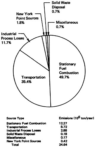
or 12.27 million tons were produced by stationary fuel combustion sources and 35.4 percent or 8.72 million tons were produced by transportation sources. All fuel combustion accounted for over 85 percent of the national total. Dissecting the data in a slightly different manner, point sources accounted for 57.3 percent (14.11 million tons) while area sources accounted for 42.7 percent (10.53 million tons) of the total national emissions. The major portion of the point source emissions was contributed by stationary fuel combustion and industrial process losses (97 percent) and the major portion of area source emissions was contributed by transportation sources (83 percent).
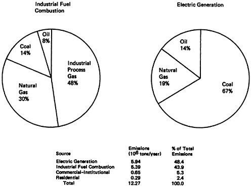
Since stationary fuel combustion sources accounted about half of the total national emissions in 1972, it is appropriate to examine the types of stationary sources and fuels which make the major contribution to stationary fuel combustion emissions. As shown in Table 14–5 and Figure 14–13, electric power generation (48 percent) and industrial fuel combustion (44 percent) shared almost equally in the production of over 92 percent of the stationary fuel combustion emissions. However, a look at the type of fuel consumed in electrical power generation and industrial heating discloses differences. Coal accounted for 67 percent of the NOx emissions from electric power generation, but only 14 percent of the industrial fuel combustion emissions. The major contributor to industrial fuel combustion NOx emissions was industrial process gas, such as coke oven gas and refinery gas, which accounts for 48 percent of the industrial fuel combustion emissions. Natural gas was the second largest contributor for each source type, accounting for 30 percent of industrial fuel combustion emissions and 19 percent of electric power generation emissions.
The predominance of coal-related NOx electric power generation emissions is a result of two factors. First, coal is the major fuel used in electric power generation. Secondly, coal has a higher NOx emission rate than oil or natural gas on an equivalent heat production basis as indicated in Table 14–6.
TABLE 14–5
Summary of Nationwide NOx Emissions by Source Type and Fuel Use, 1972
|
Source Type |
Emissions (106 tons/year) |
% of Total Emissions |
||||
|
Stationary Fuel Combustion |
12.27 |
|
49.7 |
|
||
|
Electric Generation |
|
5.94 |
|
|
24.1 |
|
|
Coal |
|
3.95 |
|
16.0 |
||
|
Oil |
0.85 |
3.4 |
||||
|
Natural Gas |
1.14 |
4.7 |
||||
|
Industrial Fuel COmbustion |
|
5.39 |
|
|
21.8 |
|
|
Coal |
|
0.76 |
|
3.0 |
||
|
Oil |
0.41 |
1.6 |
||||
|
Process Gas |
2.58 |
10.5 |
||||
|
Natural Gas |
1.64 |
6.7 |
||||
|
Commercial-Institutional |
|
0.65 |
|
|
2.6 |
|
|
Residential |
0.29 |
1.2 |
||||
|
Transportation |
8.72 |
|
35.4 |
|
||
|
Gasoline |
|
6.62 |
|
|
26.9 |
|
|
Diesel |
1.90 |
7.7 |
||||
|
Other |
0.20 |
0.8 |
||||
|
Industrial Process Losses |
2.88 |
|
11.7 |
|
||
|
Solid Waste Disposal |
0.18 |
0.7 |
||||
|
Miscellaneous |
0.17 |
0.7 |
||||
|
New York Point Sources |
0.42 |
1.8 |
||||
|
TOTAL |
24.64 |
100.0 |
||||
Projected increases in energy demand coupled a desire to convert existing electric utilities from oil and natural gas to coal combustion and to require new electric utilities to burn coal could result in a substantial increase in NOx emissions from electric power generation in the future.
Geographical Nitrogen Oxide Emission Patterns
General Patterns
Geographical nitrogen oxide emission patterns were determined by summarizing NOx emission data for all the AQCR’s and states located within the jurisdictional boundaries of each of the Environmental Protection Agency’s (EPA) 10 regional offices. A complete listing of the states located within the jurisdictional boundaries of each EPA regional office is given in Table 14–7.
Table 14–8 displays the geographical distribution of 1972 NOx emissions for the United States. The North-east includes all states east of the Mississippi River and north of the Mason-Dixon line, the South includes all states south of the Mason-Dixon line and east of Arizona, and the West includes all of the area west of the Mississippi River and north of Oklahoma and Arkansas. The North-east was responsible for 56 percent of total U.S. NOx emissions with the South and West being nearly equal contributors to the remaining 44 percent. Distribution of stationary fuel combustion emissions followed a similar pattern. Transporation emissions followed a somewhat different pattern more closely following population patterns. The North-east accounted for 42 percent of U.S. NOx emissions from transportation while the South and West contributed 32 percent and 26 percent respectively.
A closer look at the contribution of EPA Regions to total emissions reveals that 27 percent of U.S. total NOx emissions and 39 percent of U.S. stationary fuel combustion emissions
TABLE 14–7
Listing of States Located Within Jurisdictional Boundaries of EPA Regional Offices (EPA 1972)
|
EPA Region |
States and Territories |
|
I |
Connecticut, Maine, Massachusetts, New Hampshire, Rhode Island, Vermont |
|
II |
New Jersey, New York, Puerto Rico, Virgin Islands |
|
III |
Delaware, Maryland, Pennsylvania, Virginia, West Virginia |
|
IV |
Alabama, Florida, Georgia, Kentucky, Mississippi, North Carolina, South Carolina, Tennessee |
|
V |
Illinois, Indiana, Michigan, Minnesota, Ohio, Wisconsin |
|
VI |
Arkansas, Louisiana, New Mexico, Oklahoma, Texas |
|
VII |
Iowa, Kansas, Missouri, Nebraska |
|
VIII |
Colorado, Montana, North Dakota, South Dakota, Utah, Wyoming |
|
IX |
Arizona, California, Hawaii, Nevada, American Samoa, Guam |
|
X |
Alaska, Idaho, Oregon, Washington |
TABLE 14–8
Geographical Distribution of Nitrogen Oxide Emissions, 1972a
|
Geographical Area (EPA Region)b |
% Total U.S. Emissions |
% Total U.S. Stationary Fuel Combustion Emissions |
% Total U.S. Transportation Emissions |
||||
|
EAST |
|
56 |
|
59 |
|
42 |
|
|
|
V |
|
27 |
|
38 |
|
19 |
|
III |
19 |
12 |
10 |
||||
|
II |
7 |
6 |
9 |
||||
|
I |
3 |
3 |
4 |
||||
|
SOUTH |
|
24 |
|
23 |
|
32 |
|
|
|
IV |
|
14 |
|
14 |
|
19 |
|
VI |
10 |
9 |
13 |
||||
|
WEST |
|
20 |
|
18 |
|
26 |
|
|
|
IV |
|
10 |
|
10 |
|
12 |
|
VII |
5 |
5 |
7 |
||||
|
VIII |
3 |
2 |
4 |
||||
|
X |
2 |
1 |
3 |
||||
|
aPercentages have been rounded off bRegions listed in decreasing order of contribution to Area emissions. |
|||||||
were produced in the six Eastern states located in Region V. Regional transportation emissions were consistent with population distribution. Stationary fuel combustion emissions on the other hand, reflected geographical differences in industrialization and electric power requirements.
NOx Emission Patterns in EPA Regions
Tables 14–9 through 14–20 compare the distribution of NOx emissions in each of the ten EPA Regions. The Regional NOx emissions are dissected according to the degree of urbanization is determined by the largest Standard Metropolitan Statistical Area (SMSA) population within an AQCR’s are grouped in the following manner: grouped in the following manner:
-
large urban AQCR’s: AQCR’s with an SMSA population greater than 1 million;
-
medium-sized urban AQCR’s: AQCR’s with an SMSA population of 250,000–1,000,000
-
small urban AQCR’s: AQCR’s with an SMSA population of 50,000–250,000; and
-
rural AQCR’s: AQCR’s not containing an SMSA.
Although it reflects the obvious distribution of population, electric power generation and industrialization, Table 14–9 reveals some interesting points:
-
Region VIII had high rural emissions due to electric power generation. Electric generation emissions were 62 percent of rural emissions and 25 percent of the Region’s total emissions. This reflects the presence of the Four Corners power plant in Region VIII.
-
In Region X the rural emissions were also high. However, 66 percent of the emissions
TABLE 14–9
Effect of Urbanization on Nitrogen Oxide Emissions for Different Geographical Areasa,b
TABLE 14–10
1972 NOx Emissions
EPA Region I
|
Air Quality Control Regions |
||||||||||||||||||
|
Source Category |
Rural (7)a |
Medium-Sized, Urban (3)a |
Total Urban |
Total Region |
||||||||||||||
|
Tons |
% |
Tons |
% |
Tons |
% |
Ton |
% |
Tons |
% |
Tons |
% |
|||||||
|
Stationary Fuel Combustion |
20632 |
33 |
100 |
89116 |
48 |
100 |
158335 |
51 |
100 |
98664 |
59 |
100 |
346115 |
52 |
100 |
366747 |
50 |
100 |
|
Residential |
2790 |
|
13 |
5657 |
|
6 |
8000 |
|
5 |
5918 |
|
6 |
19575 |
|
6 |
22365 |
|
6 |
|
Electric Generation |
3359 |
16 |
48298 |
54 |
90825 |
57 |
47617 |
48 |
186740 |
54 |
190099 |
52 |
||||||
|
Industrial |
10785 |
52 |
20407 |
23 |
19271 |
12 |
6581 |
7 |
46259 |
13 |
57044 |
16 |
||||||
|
Commercial-Institutional |
3695 |
18 |
14754 |
17 |
40239 |
25 |
38548 |
39 |
93541 |
27 |
97236 |
26 |
||||||
|
Industrial Process Losses |
23 |
0 |
|
1041 |
1 |
|
184 |
0 |
|
0 |
0 |
|
1225 |
0 |
|
1248 |
0 |
|
|
Solid Waste Disposal |
1254 |
2 |
3816 |
2 |
4105 |
1 |
1058 |
1 |
8979 |
1 |
10233 |
1 |
||||||
|
Transportation |
41654 |
66 |
100 |
90528 |
49 |
100 |
148409 |
48 |
100 |
68830 |
41 |
100 |
307767 |
46 |
100 |
349421 |
48 |
100 |
|
Light-duty gas vehicles |
27778 |
|
67 |
64178 |
|
71 |
102637 |
|
69 |
56075 |
|
81 |
222890 |
|
72 |
250668 |
|
72 |
|
Other |
13876 |
33 |
26350 |
29 |
45772 |
31 |
12755 |
19 |
84877 |
28 |
98753 |
28 |
||||||
|
Miscellaneous |
0 |
0 |
|
0 |
0 |
|
0 |
0 |
|
0 |
0 |
|
0 |
0 |
|
0 |
0 |
|
|
Total |
63564 |
100 |
184500 |
100 |
311032 |
100 |
168553 |
100 |
664085 |
100 |
727649 |
100 |
||||||
|
a Number in parentheses indicates the number of AQCR’s in that category b Largest SMSA population within AQCR c Total urban=emissions from all AQCR’s except Rural AQCR’s |
||||||||||||||||||
TABLE 14–11
1972 NOx Emissions
EPA Region IId
|
Air Quality Control Regions |
||||||||||||||||||
|
Source Category |
Rural (2)a |
Total Urbanc |
Total Region |
|||||||||||||||
|
Tons |
% |
Tons |
% |
Tons |
% |
Tons |
% |
Tons |
% |
Tons |
% |
|||||||
|
Stationary Fuel Combustion |
9516 |
18 |
100 |
31985 |
58 |
100 |
35120 |
18 |
100 |
317296 |
36 |
100 |
384401 |
34 |
100 |
393917 |
33 |
100 |
|
Residential |
1797 |
|
19 |
819 |
|
3 |
7208 |
|
21 |
39896 |
|
13 |
47923 |
|
12 |
49720 |
|
13 |
|
Electric Generation |
824 |
9 |
22884 |
72 |
0 |
0 |
139924 |
44 |
162808 |
42 |
163632 |
42 |
||||||
|
Industrial |
713 |
7 |
2851 |
9 |
0 |
0 |
57939 |
18 |
60790 |
16 |
61503 |
16 |
||||||
|
Commercial-Institutional |
6181 |
65 |
5431 |
17 |
27913 |
79 |
79538 |
25 |
112882 |
29 |
119063 |
30 |
||||||
|
Industrial Process Losses |
0 |
0 |
|
402 |
0.7 |
|
0 |
0 |
|
23335 |
3 |
|
23737 |
2 |
|
23737 |
2 |
|
|
Solid Waste Disposal |
706 |
1 |
240 |
0.4 |
3261 |
2 |
15523 |
2 |
19024 |
2 |
19730 |
2 |
||||||
|
Transportation |
41843 |
80 |
100 |
22512 |
41 |
100 |
161947 |
81 |
100 |
511706 |
59 |
100 |
696165 |
62 |
100 |
738008 |
63 |
100 |
|
Light Duty gas vehicles |
25126 |
|
60 |
11325 |
|
50 |
96189 |
|
59 |
341373 |
|
67 |
448887 |
|
64 |
474013 |
|
64 |
|
Other |
16717 |
40 |
11187 |
50 |
65758 |
41 |
170333 |
33 |
247278 |
36 |
263995 |
36 |
||||||
|
Miscellaneous |
0 |
0 |
|
0 |
0 |
|
0 |
0 |
|
2145 |
0 |
|
2145 |
0 |
|
2145 |
0 |
|
|
Total |
52064 |
100 |
55139 |
100 |
200329 |
100 |
870005 |
100 |
1125473 |
100 |
1177537 |
100 |
||||||
|
a Number in parentheses indicates the number of AQCR’s in that category b Largest SMSA population within AQCR c Total urban=emissions from all AQCR’s except Rural AQCR’s d Does not include 421,000 tons from New York City Point Sources. |
||||||||||||||||||
TABLE 14–12
1972 NOx Emissions
EPA Region III
|
Air Quality Control Regions |
|||||||||||||||||||
|
Source Category |
Rural (12)a |
Total Urbanc |
Total Region |
||||||||||||||||
|
Tons |
% |
Tons |
% |
Tons |
% |
Tons |
% |
Tons |
% |
Tons |
% |
||||||||
|
Stationary Fuel Combustion |
200902 |
65 |
100 |
219192 |
73 |
100 |
422045 |
61 |
100 |
723466 |
22 |
100 |
1364703 |
31 |
100 |
1565605 |
34 |
100 |
|
|
Residential |
4515 |
|
2 |
3389 |
|
1 |
11185 |
|
3 |
19096 |
|
3 |
33670 |
|
2 |
38185 |
|
2 |
|
|
Electric Generation |
156591 |
78 |
162769 |
74 |
301993 |
72 |
496032 |
69 |
960794 |
70 |
1117385 |
71 |
|||||||
|
Industrial |
35347 |
18 |
49738 |
23 |
85460 |
20 |
146640 |
20 |
281838 |
21 |
317185 |
20 |
|||||||
|
Commercial-Institutional |
4559 |
2 |
3926 |
1.7 |
23407 |
6 |
61697 |
9 |
89030 |
7 |
93589 |
6 |
|||||||
|
Industrial Process Losses |
2025 |
0.6 |
|
6210 |
2 |
|
4524 |
0.6 |
|
2175857 |
65 |
|
2186591 |
50 |
|
2188616 |
47 |
|
|
|
Solid Waste Disposal |
1749 |
0.5 |
1259 |
0.4 |
1341 |
0.2 |
6312 |
0.1 |
8912 |
0.2 |
10661 |
0.2 |
|||||||
|
Transportation |
103413 |
34 |
100 |
75748 |
25 |
100 |
265678 |
38 |
100 |
439907 |
13 |
100 |
781333 |
18 |
100 |
884746 |
19 |
100 |
|
|
Light-duty gas vehicles |
59474 |
|
58 |
43950 |
|
58 |
160580 |
|
60 |
266356 |
|
61 |
470886 |
|
60 |
530360 |
|
60 |
|
|
Other |
43939 |
42 |
31798 |
42 |
105098 |
40 |
173551 |
39 |
310447 |
40 |
354386 |
40 |
|||||||
|
Miscellaneous |
56 |
.01 |
|
0 |
0 |
|
0 |
0 |
|
4 |
0 |
|
4 |
0 |
|
60 |
0 |
|
|
|
Total |
308147 |
100 |
302410 |
100 |
693,587 |
100 |
3345546 |
100 |
4341543 |
100 |
4649690 |
100 |
|||||||
|
a Number in parentheses indicates the number of AQCR’s in that category b Largest SMSA Population within AQCR c Total urban=emissions from all AQCR’s except Rural AQCR’s |
|||||||||||||||||||
TABLE 14–13
1972 NOx Emissions
EPA Region IV
|
Air Quality Control Regions |
||||||||||||||||||
|
Source Category |
Rural (16)a |
Total Urbanc |
Total Region |
|||||||||||||||
|
Tons |
% |
Tons |
% |
Tons |
% |
Tons |
% |
Tons |
% |
Tons |
% |
|||||||
|
Stationary Fuel Combustion |
156522 |
31 |
100 |
376839 |
52 |
100 |
950265 |
52 |
100 |
237407 |
49 |
100 |
1564511 |
51 |
100 |
1721033 |
48 |
100 |
|
Residential |
6672 |
|
4 |
8115 |
|
2 |
11984 |
|
1 |
1646 |
|
1 |
21739 |
|
1 |
28411 |
|
2 |
|
Electric Generation |
97421 |
62 |
247034 |
66 |
689749 |
73 |
184154 |
77 |
1102937 |
70 |
1218358 |
71 |
||||||
|
Industrial |
43360 |
28 |
111834 |
30 |
220141 |
23 |
45886 |
19 |
377861 |
24 |
421221 |
24 |
||||||
|
Commercial-Institutional |
9066 |
6 |
9858 |
3 |
28393 |
3 |
5726 |
2 |
43977 |
3 |
53043 |
3 |
||||||
|
Industrial Process Losses |
9072 |
2 |
|
9180 |
1 |
|
67525 |
4 |
|
5539 |
1 |
|
82244 |
3 |
|
91316 |
3 |
|
|
Solid Waste Disposal |
6359 |
1 |
8169 |
1 |
12670 |
1 |
2332 |
1 |
23171 |
1 |
29530 |
1 |
||||||
|
Transportation |
338750 |
66 |
100 |
329640 |
46 |
100 |
804008 |
44 |
100 |
234761 |
49 |
100 |
1368409 |
45 |
100 |
1707159 |
48 |
100 |
|
Light-duty gas vehicles |
243307 |
|
72 |
199124 |
|
60 |
589073 |
|
73 |
146702 |
|
62 |
934899 |
|
68 |
1178206 |
|
69 |
|
Other |
95443 |
28 |
130156 |
40 |
214935 |
27 |
88059 |
38 |
433510 |
32 |
528953 |
31 |
||||||
|
Miscellaneous |
1076 |
0 |
|
0 |
0 |
|
2394 |
0 |
|
1974 |
0 |
|
4368 |
0 |
|
5444 |
0 |
|
|
Total |
511776 |
100 |
723834 |
100 |
1837044 |
100 |
482016 |
100 |
3042894 |
100 |
3554670 |
100 |
||||||
|
a Number in parentheses indicates the number of AQCR’s in that category b Largest SMSA population within AQCR’s except Rural AQCR’s c Total urban=emissions from all AQCR’s except Rural AQCR’s |
||||||||||||||||||
TABLE 14–14
1972 NOx Emissions
EPA Region V
|
Air Quality Control Regions |
||||||||||||||||||
|
Source Category |
Rural (13)a |
Total Urbanc |
Total Region |
|||||||||||||||
|
Tons |
% |
Tons |
% |
Tons |
% |
Tons |
% |
Tons |
% |
Tons |
% |
|||||||
|
Stationary Fuel Combustion |
550994 |
66 |
100 |
136182 |
46 |
100 |
754891 |
55 |
100 |
3375474 |
80 |
100 |
4266552 |
73 |
100 |
4817546 |
72 |
100 |
|
Residential |
9695 |
|
2 |
5694 |
|
4 |
22719 |
|
3 |
37865 |
|
1 |
66278 |
|
2 |
72973 |
|
2 |
|
Electric Generation |
441305 |
80 |
53019 |
39 |
445422 |
59 |
574867 |
17 |
1073308 |
25 |
1514613 |
31 |
||||||
|
Industrial |
84982 |
15 |
63809 |
47 |
234826 |
31 |
2693250 |
80 |
2991885 |
70 |
3076867 |
64 |
||||||
|
Commercial-Institutional |
15048 |
3 |
13657 |
10 |
51925 |
7 |
69498 |
2 |
135080 |
3 |
150128 |
3 |
||||||
|
Industrial Process Losses |
47450 |
6 |
|
2361 |
1 |
|
35693 |
3 |
|
51781 |
1 |
|
89835 |
2 |
|
137285 |
2 |
|
|
Solid Waste Disposal |
3399 |
0.4 |
3004 |
1 |
9946 |
1 |
21970 |
1 |
34920 |
1 |
38319 |
1 |
||||||
|
Transportation |
231182 |
28 |
100 |
151566 |
52 |
100 |
562855 |
|
100 |
727989 |
17 |
100 |
1442410 |
25 |
100 |
1673592 |
25 |
100 |
|
Light-duty gas vehicles |
121864 |
|
53 |
79263 |
|
52 |
294859 |
|
52 |
438331 |
|
60 |
812453 |
|
56 |
934317 |
|
56 |
|
Other |
109318 |
47 |
72303 |
48 |
267996 |
48 |
289658 |
40 |
629957 |
44 |
739275 |
44 |
||||||
|
Miscellaneous |
2 |
0 |
|
0 |
0 |
|
0 |
0 |
|
1 |
0 |
|
1 |
|
|
3 |
0 |
|
|
Total |
832307 |
100 |
293103 |
100 |
1363388 |
100 |
4197602 |
100 |
5854093 |
100 |
6686400 |
100 |
||||||
|
a Number in parentheses indicates the number of AQCR’s in that category b Largest SMSA population within AQCR c Total urban=emissions from all AQCR’s except Rural AQCR’s |
||||||||||||||||||
TABLE 14–15
1972 NOx Emissions
EPA Region VI
|
Air Quality Control Regions |
||||||||||||||||||
|
Source Category |
Rural (9)a |
Total Urbanc |
Total Region |
|||||||||||||||
|
Tons |
% |
Tons |
% |
Tons |
% |
Tons |
% |
Tons |
% |
Tons |
% |
|||||||
|
Stationary Fuel Combustion |
72887 |
38 |
100 |
157265 |
40 |
100 |
417050 |
50 |
100 |
488012 |
48 |
100 |
1062327 |
47 |
100 |
1135214 |
47 |
100 |
|
Residential |
2510 |
|
3 |
7711 |
|
5 |
6385 |
|
2 |
5527 |
|
1 |
19623 |
|
2 |
22133 |
|
2 |
|
Electric Generation |
38846 |
53 |
81637 |
52 |
201899 |
48 |
301193 |
62 |
584729 |
55 |
623575 |
55 |
||||||
|
Industrial |
28789 |
39 |
62068 |
39 |
194014 |
47 |
163377 |
33 |
419459 |
39 |
448248 |
39 |
||||||
|
Commercial-Institutional |
2744 |
4 |
5838 |
4 |
14751 |
4 |
17915 |
4 |
38504 |
4 |
41248 |
4 |
||||||
|
Industrial Process Losses |
4736 |
2 |
|
28701 |
7 |
|
25989 |
3 |
|
123458 |
12 |
|
178148 |
8 |
|
182884 |
7 |
|
|
Solid Waste Disposal |
2127 |
1 |
3396 |
1 |
6610 |
1 |
8825 |
1 |
18831 |
1 |
20958 |
1 |
||||||
|
Transportation |
113393 |
59 |
100 |
207023 |
52 |
100 |
387972 |
46 |
100 |
386572 |
38 |
100 |
981567 |
44 |
100 |
1094960 |
45 |
100 |
|
Light-duty gas vehicles |
55143 |
|
49 |
90624 |
|
44 |
198071 |
|
51 |
205388 |
|
53 |
494083 |
|
51 |
549226 |
|
50 |
|
Other |
58250 |
51 |
116399 |
56 |
189901 |
49 |
181184 |
47 |
487484 |
49 |
545734 |
50 |
||||||
|
Miscellaneous |
0 |
0 |
|
0 |
0 |
|
0 |
0 |
|
0 |
0 |
|
0 |
0 |
|
0 |
0 |
|
|
Total |
193143 |
100 |
396375 |
100 |
837620 |
100 |
1012866 |
100 |
2246861 |
100 |
2440004 |
100 |
||||||
|
a Number in parentheses indicates the number of AQCR’s in that category b Largest SMSA population within AQCR c Total urban=emissions from all AQCR’s except Rural AQCR’s |
||||||||||||||||||
TABLE 14–16
1972 NOx Emissions
EPA Region VII
|
Air Quality Control Regions |
||||||||||||||||||
|
Source Category |
Rural (10)a |
Total Urbanc |
Total Region |
|||||||||||||||
|
Tons |
% |
Tons |
% |
Tons |
% |
Tons |
% |
Tons |
% |
Tons |
% |
|||||||
|
Stationary Fuel Combustion |
90687 |
32 |
100 |
195354 |
46 |
100 |
16667 |
41 |
100 |
375130 |
67 |
100 |
587151 |
57 |
100 |
677838 |
51 |
100 |
|
Residential |
4731 |
|
5 |
6176 |
|
3 |
616 |
|
4 |
4916 |
|
1 |
11708 |
|
2 |
16439 |
|
2 |
|
Electric Generation |
54077 |
60 |
146372 |
75 |
12879 |
77 |
327690 |
87 |
486941 |
83 |
541018 |
80 |
||||||
|
Industrial |
24567 |
27 |
30833 |
16 |
1539 |
9 |
35877 |
10 |
68249 |
12 |
92816 |
14 |
||||||
|
Commercial-Institutional |
7311 |
8 |
11975 |
6 |
1633 |
10 |
6647 |
2 |
20255 |
3 |
27566 |
4 |
||||||
|
Industrial Process Losses |
8530 |
3 |
|
11695 |
3 |
|
1354 |
3 |
|
15619 |
3 |
|
28668 |
3 |
|
37198 |
3 |
|
|
Solid Waste Disposal |
2926 |
1 |
3991 |
1 |
216 |
0.5 |
2470 |
0.4 |
6677 |
0.6 |
9603 |
1 |
||||||
|
Transportation |
184239 |
64 |
100 |
214704 |
50 |
100 |
21855 |
54 |
100 |
170659 |
30 |
100 |
407218 |
40 |
100 |
591457 |
45 |
100 |
|
Light-duty gas vehicles |
84109 |
|
46 |
111437 |
|
52 |
13191 |
|
60 |
96782 |
|
57 |
221410 |
|
54 |
305519 |
|
52 |
|
Other |
100130 |
54 |
103267 |
48 |
8664 |
40 |
73877 |
43 |
185808 |
46 |
285938 |
48 |
||||||
|
Miscellaneous |
745 |
0.2 |
|
356 |
0.1 |
|
80 |
0.1 |
|
0 |
0 |
|
436 |
.04 |
|
1181 |
0.1 |
|
|
Total |
287126 |
100 |
426102 |
100 |
40172 |
100 |
563877 |
100 |
1030151 |
100 |
1317277 |
100 |
||||||
|
a Number in parentheses indicates the number of AQCR’s in that category b Largest SMSA population within AQCR c Total urban=emissions from all AQCR’s except Rural AQCR’s |
||||||||||||||||||
TABLE 14–17
1972 NOx Emissions
EPA Region VIII
|
Air Quality Control Regions |
||||||||||||||||||
|
Source Category |
Rural (16)a |
Total Urbanc |
Total Region |
|||||||||||||||
|
Tons |
% |
Tons |
% |
Tons |
% |
Tons |
% |
Tons |
% |
Tons |
% |
|||||||
|
Stationary Fuel Combustion |
229297 |
51 |
100 |
31325 |
18 |
100 |
21900 |
38 |
100 |
30194 |
37 |
100 |
83419 |
26 |
100 |
312716 |
41 |
100 |
|
Residential |
5390 |
|
2 |
1394 |
|
4 |
1288 |
|
6 |
1441 |
|
5 |
4123 |
|
5 |
9513 |
|
3 |
|
Electric Generation |
187860 |
82 |
11847 |
38 |
6298 |
29 |
18192 |
60 |
36337 |
44 |
224197 |
72 |
||||||
|
Industrial |
27406 |
12 |
14400 |
46 |
10647 |
49 |
6696 |
22 |
31743 |
38 |
59149 |
19 |
||||||
|
Commercial-Institutional |
8704 |
4 |
3685 |
12 |
3667 |
17 |
3863 |
13 |
11215 |
13 |
19919 |
6 |
||||||
|
Industrial Process Losses |
7976 |
2 |
|
91591 |
51 |
|
5095 |
9 |
|
4726 |
6 |
|
101412 |
32 |
|
109388 |
14 |
|
|
Solid Waste Disposal |
2864 |
1 |
691 |
0 |
329 |
1 |
188 |
0 |
1208 |
0 |
4072 |
1 |
||||||
|
Transportation |
203745 |
46 |
100 |
54018 |
30 |
100 |
30581 |
53 |
100 |
47469 |
57 |
100 |
132068 |
41 |
100 |
335813 |
44 |
100 |
|
Light-duty gas vehicles |
92125 |
|
45 |
27671 |
|
51 |
18981 |
|
62 |
29631 |
|
62 |
76283 |
|
58 |
168408 |
|
50 |
|
Other |
111620 |
55 |
26347 |
49 |
11600 |
38 |
17838 |
38 |
55785 |
42 |
167405 |
50 |
||||||
|
Miscellaneous |
3780 |
1 |
|
434 |
0 |
|
10 |
0 |
|
0 |
0 |
|
444 |
0 |
|
4224 |
1 |
|
|
Total |
447700 |
100 |
178059 |
100 |
57916 |
100 |
82578 |
100 |
318553 |
100 |
766253 |
100 |
||||||
|
a Number in parentheses indicates the number of AQCR’s in that category b Largest SMSA population within AQCR c Total urban=emissions from all AQCR’s except Rural AQCR’s |
||||||||||||||||||
TABLE 14–18
1972 NOx Emissions
EPA Region IX
|
Air Quality Control Regions |
||||||||||||||||||
|
Source Category |
Rural (12)a |
Total Urbanc |
Total Region |
|||||||||||||||
|
Tons |
% |
Tons |
% |
Tons |
% |
Tons |
% |
Tons |
% |
Tons |
% |
|||||||
|
Stationary Fuel Combustion |
156693 |
55 |
100 |
5177 |
42 |
100 |
155213 |
33 |
100 |
882293 |
57 |
100 |
1042683 |
51 |
100 |
1199376 |
52 |
100 |
|
Residential |
1915 |
|
1 |
255 |
|
5 |
4164 |
|
3 |
12172 |
|
1 |
16591 |
|
2 |
18506 |
|
2 |
|
Electric Generation |
112924 |
72 |
4259 |
82 |
121888 |
78 |
182969 |
21 |
309116 |
30 |
422040 |
35 |
||||||
|
Industrial |
39254 |
25 |
0 |
0 |
19381 |
12 |
660586 |
75 |
679967 |
65 |
719221 |
60 |
||||||
|
Commercial-Institutional |
2604 |
2 |
662 |
13 |
9781 |
7 |
26568 |
4 |
37011 |
4 |
39615 |
3 |
||||||
|
Industrial Process Losses |
13167 |
5 |
|
1 |
0 |
|
3804 |
0.5 |
|
62140 |
4 |
|
65945 |
3 |
|
79112 |
3 |
|
|
Solid Waste Disposal |
2703 |
1 |
5 |
0 |
7368 |
2 |
17189 |
1 |
24562 |
1 |
27265 |
1 |
||||||
|
Transportation |
110240 |
39 |
100 |
7049 |
|
100 |
304801 |
64 |
100 |
589829 |
38 |
100 |
901679 |
44 |
100 |
1011919 |
44 |
100 |
|
Light-duty gas vehicles |
51967 |
|
47 |
4342 |
|
62 |
163512 |
|
54 |
381100 |
|
65 |
548954 |
|
61 |
600921 |
|
59 |
|
Other |
58273 |
53 |
2707 |
38 |
141289 |
46 |
208729 |
35 |
352725 |
39 |
410998 |
41 |
||||||
|
Miscellaneous |
0 |
0 |
|
0 |
0 |
|
2611 |
.5 |
|
0 |
0 |
|
2611 |
0 |
|
2611 |
0 |
|
|
Total |
282820 |
100 |
12232 |
100 |
473794 |
100 |
1551453 |
100 |
2037479 |
100 |
2320299 |
100 |
||||||
|
a Number in parentheses indicates the number of AQCR’s in that category b Largest SMSA population within AQCR c Total urban=emissions from all AQCR’s except Rural AQCR’s |
||||||||||||||||||
TABLE 14–19
1972 NOx Emissions
EPA Region X
|
Air Quality Control Regions (Washington, Oregon, Idaho) |
||||||||||||||||||
|
Source Category |
Rural (8)a |
Total Urbanc |
Total Region |
|||||||||||||||
|
Tons |
% |
Tons |
% |
Tons |
% |
Tons |
% |
Tons |
% |
Tons |
% |
|||||||
|
Stationary Fuel Combustion |
32346 |
21 |
100 |
5192 |
21 |
100 |
4673 |
47 |
100 |
37512 |
21 |
100 |
47377 |
22 |
100 |
79723 |
22 |
100 |
|
Residential |
3283 |
|
10 |
500 |
|
10 |
277 |
|
6 |
4386 |
|
12 |
5163 |
|
11 |
8446 |
|
11 |
|
Electric Generation |
0 |
0 |
0 |
0 |
0 |
0 |
313 |
1 |
313 |
1 |
313 |
0 |
||||||
|
Industrial |
27772 |
86 |
4328 |
83 |
4239 |
91 |
28285 |
75 |
36852 |
78 |
64624 |
81 |
||||||
|
Commercial-Institutional |
1286 |
4 |
363 |
7 |
156 |
3 |
4519 |
12 |
5038 |
11 |
6324 |
8 |
||||||
|
Industrial Process Losses |
13337 |
9 |
|
0 |
0 |
|
0 |
0 |
|
1509 |
1 |
|
1509 |
1 |
|
14846 |
4 |
|
|
Solid Waste Disposal |
2193 |
1 |
329 |
1 |
214 |
2 |
3325 |
2 |
3868 |
2 |
6061 |
2 |
||||||
|
Transportation |
100035 |
66 |
100 |
19179 |
76 |
100 |
5027 |
51 |
100 |
137280 |
76 |
100 |
161486 |
74 |
100 |
261521 |
71 |
100 |
|
Light-duty gas vehicles |
48796 |
|
49 |
8816 |
|
46 |
2777 |
|
55 |
77714 |
|
57 |
89307 |
|
55 |
138103 |
|
53 |
|
Other |
51239 |
51 |
10363 |
54 |
2250 |
45 |
59566 |
43 |
72179 |
45 |
123418 |
47 |
||||||
|
Miscellaneous |
2858 |
2 |
|
483 |
2 |
|
21 |
0 |
|
2071 |
1 |
|
2575 |
1 |
|
5433 |
1 |
|
|
Total |
150770 |
100 |
25184 |
100 |
9934 |
100 |
181697 |
100 |
216815 |
100 |
367585 |
100 |
||||||
|
a Number in parentheses indicates the number of AQCR’s in that category b Largest SMSA population within AQCR c Total urban=emissions from all AQCR’s except Rural AQCR’s |
||||||||||||||||||
TABLE 14–20
1972 NOx Emissions
EPA Region X
|
Air Quality Control Regions (Alaska) |
||||||||||||||||||
|
Source Category |
Rural (1)a |
Total Urbanc |
Total Region |
|||||||||||||||
|
Tons |
% |
Tons |
% |
Tons |
% |
Tons |
% |
Tons |
% |
Tons |
% |
|||||||
|
Stationary Fuel Combustion |
20,873 |
58 |
100 |
|
|
100 |
|
|
100 |
|
|
100 |
|
|
100 |
20873 |
58 |
100 |
|
Residential |
1095 |
|
5 |
|
1095 |
|
53 |
|||||||||||
|
Electric Generation |
7022 |
34 |
7022 |
34 |
||||||||||||||
|
Industrial |
9513 |
46 |
9513 |
46 |
||||||||||||||
|
Commercial-Institutional |
3243 |
16 |
3243 |
16 |
||||||||||||||
|
Industrial Process Losses |
0 |
0 |
|
0 |
0 |
|
||||||||||||
|
Solid Waste Disposal |
776 |
2 |
776 |
2 |
||||||||||||||
|
Transportation |
14459 |
40 |
100 |
|
|
100 |
|
|
100 |
|
|
100 |
|
|
100 |
14459 |
40 |
100 |
|
Light-duty gas vehicles |
3879 |
|
27 |
|
3879 |
|
27 |
|||||||||||
|
Other |
10580 |
73 |
10580 |
73 |
||||||||||||||
|
Miscellaneous |
0 |
0 |
|
0 |
0 |
|
||||||||||||
|
Total |
36108 |
100 |
|
|
100 |
|
|
100 |
|
|
100 |
|
|
100 |
|
36108 |
100 |
|
|
a Number in parentheses indicates the number of AQCR’s in that category b Largest SMSA population within AQCR c Total urban=emissions from all AQCR’s except Rural AQCR’s |
||||||||||||||||||
-
were transporation related. Surprisingly, this represented 27 percent of the total Region’s emissions. Further, rural industrial fuel combustion emissions equaled urban industrial fuel combustion emissions in this Region.
-
In Region II 81 percent of emissions arose in three large urban AQCR’s. The transportation emissions in just these large urban AQCR’s represented 43 percent of the Region’s total emissions. Stationary fuel combustion in these largest urban AQCR’s generated 27 percent of the Region’s emissions with only 12 percent coming from electric power generation.
-
In Region III the urban emissions were dominated by industrial processing. Forty-six percent of the Region’s emissions arose from industrial processing in a single AQCR, the Metropolitan Philadelphia Interstate AQCR. (This is due, at least in part, to the fact that petroleum refinery emissions have been carefully surveyed in the Philadelphia area, as discussed earlier in this chapter.)
-
In Region I transportation emissions are dominated by light duty gasoline vehicles (72 percent). For all other Regions, light duty gas line vehicles contribute an average of 57 percent of the transportation emissions.
There are some similarities among Regions in the distribution of emissions which reflect the degree of urbanization and industrialization of the Regions:
-
Regions I and IV (New England and the Southeast) had a similar distribution of emissions between rural and urban AQCR’s. The majority of the Regional emissions were produced in medium-sized urban AQCR’s. However, Southern states had a greater proportion of electric power emissions in rural areas.
-
Regions II, III, and V represent major population centers. Sixty-three to 80 percent of the Regions’ emissions were produced in large urban areas.
Effects of Degree of Urbanization on Nationwide Nitrogen Oxide Emissions
Figure 14–14 displays the effects of the degree of urbanization on nationwide NOx emissions in 1972. Urban AQCR’s accounted for 87 percent of the total NOx emissions. Large urban AQCR’s alone accounted for 53 percent of total emissions while rural AQCR’s contributed only 13 percent of total emissions. Thus, the major portion of the NOx problem as characterized by NOx emissions was in urban areas.
Analysis of the 10 AQCR’s with the largest SMSA populations indicates that these AQCR’s accounted for 39 percent of the total U.S. NOx emissions. The emissions from these ten AQCR’s are shown in Table 14–21. The majority of the emissions in these AQCR’s were produced by stationary fuel combustion and industrial process loss sources with transportation sources contributing only 20 percent of the total. This is in marked contrast to the remainder of the country where transportation contributed 45 percent of total emissions.
Nitrogen Oxide Emissions by States
Table 14–22 ranks the states and the District of Columbia according to their total statewide NOx emissions. Table 14–22 also provides another basis for characterizing NOx emissions; it compares emissions per capita and emissions per unit area for each state to the NOx emission density for the contiguous United States. The U.S. NOx emission density is approximately 8.15 tons per square mile and National emissions per capita are approximately 0.112 tons.
The column labeled Ratio Emission Densities (State/U.S.) in Table 14–22 presents a tabulation of each state’s NOx emissions per square mile divided by 8.15 tons per square mile, the nationally averaged emission density. The ratios range from 104 for the District of Columbia to .008 for Alaska. The states of Pennsylvania, Michigan, Indiana, New Jersey, Massachusetts, Maryland and Rhode Island had NOx emission den-
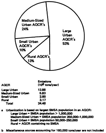
TABLE 14–21
1972 NOx Emissions from 10 Largest Urban Air Quality Control Regionsa
|
AQCRb (Name of Largest City) |
Total Emissions (106 tons/year) |
Stationary Fuel Combustion Emissions (106 tons/year) |
Transportation Emissions (106 tons/year) |
Other Sources |
|
New York-New Jersey-Connecticut Interstate |
1.15 |
0.69 |
0.43 |
0.11 |
|
Metropolitan Los Angeles Intrastate |
1.20 |
0.79 |
0.36 |
0.05 |
|
Metropolitan Chicago Interstate |
1.33 |
1.07 |
0.23 |
0.03 |
|
Metropolitan Philadelphia Interstate |
2.58 |
0.24 |
0.18 |
2.16c |
|
San Francisco Bay Area Intrastate |
0.28 |
0.06 |
0.19 |
0.03 |
|
Metropolitan Detroit-Port Huron Intrastate |
2.01 |
1.85 |
0.15 |
0.01 |
|
Greater Metropolitan Cleveland Intrastate |
0.29 |
0.15 |
0.13 |
0.01 |
|
Metropolitan Boston Intrastate |
0.17 |
0.09 |
0.07 |
0.01 |
|
National Capitol Interstate (Washington, D.C.) |
0.18 |
0.09 |
0.09 |
0 |
|
Metropolitan St. Louis Interstate |
0.43 |
0.31 |
0.11 |
0.01 |
|
TOTAL |
9.62 |
5.26 |
1.94 |
2.42 |
|
aAQCR’s chosen by SMSA population bAQCR’s listed in descending order of SMSA population cDue to industrial process emissions |
||||
TABLE 14–22
NOx Emissions by States and the District of Columbia
|
Rank |
State |
State’s Emissions |
Running % U.S. Total |
Ratio Emission Densities (State/US) |
Ratio Emission Capita (State/US) |
|
1 |
Pennsylvania |
3,326,053 |
13 |
9.1 |
2.5 |
|
2 |
Michigan |
2,449,819 |
22.9 |
5.3 |
2.5 |
|
3 |
California |
1,833,297 |
30.9 |
1.4 |
.82 |
|
4 |
New York |
1,659,019 |
37.6 |
2.7 |
.52 |
|
5 |
Indiana |
1,511,526 |
43.7 |
5.1 |
2.6 |
|
6 |
Texas |
1,427,195 |
49.6 |
.67 |
1.2 |
|
7 |
Ohio |
1,214,163 |
54.5 |
3.6 |
.98 |
|
8 |
Illinois |
1,074,061 |
58.9 |
2.4 |
.87 |
|
9 |
Florida |
710,764 |
61.8 |
1.6 |
.94 |
|
10 |
South Carolina |
574,904 |
64.1 |
2.3 |
1.9 |
|
11 |
New Jersey |
539,268 |
66.3 |
8.8 |
.67 |
|
12 |
Missouri |
494,166 |
68.3 |
.13 |
2.1 |
|
13 |
Tennessee |
470,085 |
70.2 |
1.4 |
1.1 |
|
14 |
Louisiana |
466,076 |
72.1 |
1.3 |
1.1 |
|
15 |
Kentucky |
462,025 |
73.9 |
1.4 |
1.3 |
|
16 |
North Carolina |
454,813 |
75.8 |
.11 |
.79 |
|
17 |
Wisconsin |
450,332 |
77.6 |
1.0 |
.09 |
|
18 |
Alabama |
437,693 |
79.4 |
.03 |
.04 |
|
19 |
Georgia |
407,653 |
81 |
.86 |
.79 |
|
20 |
Massachusetts |
368,590 |
82.5 |
5.8 |
.58 |
|
21 |
Virginia |
363,000 |
84 |
1.1 |
.69 |
|
22 |
Minnesota |
343,738 |
85.4 |
.53 |
.80 |
|
Rank |
State |
State Emissions |
Running % U.S. Total |
Ratio Emission Densities (State/US) |
Ratio Emission Capita (State/US) |
|
23 |
Maryland |
293,337 |
86.6 |
7.2 |
.68 |
|
24 |
Iowa |
267,337 |
87.7 |
.59 |
.85 |
|
25 |
Kansas |
257,926 |
88.7 |
.39 |
1.0 |
|
26 |
West Virginia |
253,088 |
89.8 |
1.3 |
1.3 |
|
27 |
Oklahoma |
245,470 |
90.8 |
.44 |
.86 |
|
28 |
New Mexico |
219,559 |
91.5 |
.22 |
1.9 |
|
29 |
Washington |
207,150 |
92.2 |
.38 |
.54 |
|
30 |
Mississippi |
190,170 |
.49 |
.76 |
|
|
31 |
Arkansas |
186,278 |
|
.03 |
.06 |
|
32 |
Connecticut |
171,775 |
.56 |
.06 |
|
|
33 |
Montana |
163,588 |
.13 |
2.1 |
|
|
34 |
Colorado |
163,586 |
.19 |
.66 |
|
|
35 |
Oregon |
149,637 |
.19 |
.64 |
|
|
36 |
Arizona |
136,544 |
.15 |
.69 |
|
|
37 |
Nebraska |
112,378 |
.18 |
.68 |
|
|
38 |
Nevada |
98,032 |
.11 |
1.8 |
|
|
39 |
North Dakota |
94,477 |
.17 |
1.3 |
|
|
40 |
Utah |
89,285 |
.13 |
.71 |
|
|
41 |
Maine |
84,592 |
.34 |
.76 |
|
|
42 |
Wyoming |
79,997 |
.1 |
2.1 |
|
|
43 |
New Hampshire |
74,195 |
1.0 |
.89 |
|
|
44 |
Delaware |
64,383 |
3.9 |
1.11 |
sities over 40 tons/sq. mile. (It should be noted, however, that the Pennsylvania data include a comprehensive survey of petroleum refinery emissions near Philadelphia. Since such surveys do not exist elsewhere, emissions from states other than Pennsylvania may be greater than shown here.)
A comparison of per capita emissions is given in the column of Table 14–22 labeled Ratio Emission Capita (State/U.S.). The per capita NOx emissions range from 2.6 for Indiana to 0.4 for Alabama. Pennsylvania, Michigan, Indiana, Missouri, Montana and Wyoming had per capita emissions which were two or more times the National average of 225 pounds per person per year. Montana and Wyoming contributed less than 1 percent each to the total U.S. emissions but had a high per capita emission ratio because of their small population.
Table 14–22 also compiles the running accumulating percent contribution of state’s emissions to the total U.S. NOx emissions (24.64 million tons/year). Interestingly, six states (Pennsylvania, Michigan, California, New York, Indiana and Texas) were responsible for about 50 percent of the nationwide NOx emissions. Pennsylvania, itself, contributed over 13 percent. Over 90 percent of the annual NOx emissions are accounted for in the first 27 states listed, with the remaining 23 states and the District of Columbia combining to contribute less than 10 percent.
Nationwide NOx Emission Trends
1940–1972
Nationwide NOx emission trends from 1940–1972 are displayed in Table 14–23 and Figure 14–15 (USEPA 1973a). Total nationwide emissions tripled in the three decades from 1940–1972. The stationary source fuel combustion category revealed the largest emission growth increasing from 3.5 million tons in 1940 to 12.3 million tons in 1972. In this category, emissions from electric power generation showed the greatest increase, climbing nearly 800 percent over the three decades. Transportation emissions tripled during this period.
TABLE 14–23
Nationwide NOx Emissions, 1940–1970 (EPA 1973b)
|
|
NOx Emissions (106 tons/year) |
|||||
|
Source Category |
1940 |
1950 |
1960 |
1968 |
1969 |
1970 |
|
Stationary Fuel Combustion |
3.5 |
4.3 |
5.2 |
9.7 |
10.2 |
10.0 |
|
Electric Generation |
0.6 |
1.2 |
2.3 |
4.2 |
4.3 |
4.7 |
|
Industrial |
1.9 |
2.0 |
1.8 |
3.7 |
4.6 |
4.5 |
|
Commercial-Institutional |
0.1 |
0.1 |
0.2 |
1.0 |
0.4 |
0.2 |
|
Residential |
0.9 |
1.0 |
0.9 |
0.8 |
0.9 |
0.6 |
|
Industrial Process Losses |
<0.1 |
0.1 |
0.1 |
0.2 |
0.2 |
0.2 |
|
Solid Waste Disposal |
0.1 |
0.2 |
0.2 |
0.4 |
0.4 |
0.4 |
|
Transportation |
1.7 |
2.9 |
4.3 |
7.5 |
8.3 |
8.8 |
|
Road Vehicles |
1.4 |
2.2 |
3.5 |
5.5 |
5.8 |
6.2 |
|
Gasoline |
1.4 |
2.15 |
3.2 |
4.8 |
5.1 |
5.4 |
|
Diesel |
<0.1 |
0.05 |
0.3 |
0.7 |
0.7 |
0.8 |
|
Other |
0.3 |
0.7 |
0.8 |
2.0 |
2.5 |
2.6 |
|
Miscellaneous |
0.8 |
0.4 |
0.2 |
0.2 |
0.2 |
0.1 |
|
Total |
6.1 |
7.9 |
10.0 |
18.2 |
19.3 |
19.5 |
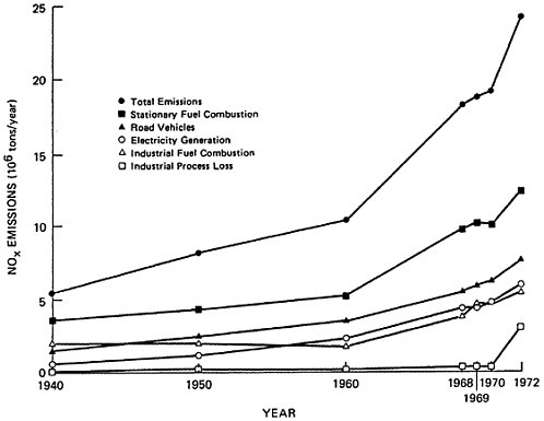
Total Emissions: 1972–1990
In Appendix 14-C, total emissions of nitrogen oxide are projected to the year 1990 under various assumptions about the implementation of regulatory programs and about the growth rate of stationary and mobile sources.
Assuming the implementation of the present statutory program for NOx control; using emission projections for electric power generation based on forecasts by the Federal Energy Administration (USEPA 1975) and the National Academy of Engineering (1974); assuming a slowing of the growth rate of NOx emissions from industrial, commercial, and institutional fuel combustion; and using other assumptions presented in detail in Appendix 14-C, a conservative estimate yields a 36 percent increase in total NOx emissions from 1972–1990 (see Figure 14–16). The largest increases will result from industrial process losses, non-highway transportation, industrial fuel combustion, and electric power generation. Highway-related transportation emissions will decline under the assumptions of this projection as Federal controls on nitrogen oxide emissions from automobiles are implemented.
Appendix 14-C examines future NOx emissions from electric power generation and highway vehicles in some detail. Protections of power generation emissions are critically dependent upon the rate at which nuclear power generation increases. If for any reason no new nuclear power plants were built after 1975, NOx emissions from power generation facilities could more than double. Road vehicle emissions are projected under three options: (1) no control of NOx emissions, (2) implementation of a proposed five year delay of the 1977 statutory standards and (3) implementation of the present statutory program. The analysis shows a 25 percent reduction in road vehicle NOx emissions by 1990 (compared with 1972) under the present statutory program (if vehicle miles of travel increase by 4 percent per year). The five year delay leads to a 17 percent reduction in emissions by 1990. Emission reductions are somewhat smaller than might be expected from the
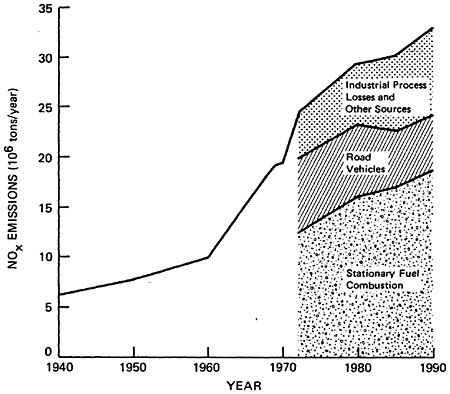
LITERATURE CITED
Altschuller, A.P. (1958) Tellus 10, 479.
Bates, D.R. and P.B.Hays (1967) Planetary Space Sci., 15, 189.
Berdyer, Kh.B, N.V.Pavlovich, and A.A. Tuzhilina (1967) Effect of Motor Vehicle Exhaust Gases on Atmospheric Pollution in Dwellings and in a Main Street, Hyg. and Sanitation (Moscow) 32:424–426, Ap-Jn.
Coffey, P.E. and W.N.Stasiuk (1975) Evidence of Atmospheric Transport of Ozone into Urban Areas, Env. Sci., and Tech., 9(1).
Commonwealth of Massachusetts (1974) Ozone Data, 1973.
Cortese, A.D. (1975) Harvard School of Public Health, Unpublished NOx Emission Estimates, January.
Council on Environmental Quality (1975) The Fifth Annual Report, 274.
Hamilton, H.L. et al. (1968) Am. Atmospheric Physics and Chemistry Study on Pikes Peak in Support of Pulmonary Edema Research RTI for Army Research Office, Research Triangle Park, N.C.
Junge, C.E. (1956) Recent Investigations in Air Chemistry, Tellus 8:127–139, May.
Junge, C.E. (1963) Air Chemistry and Radioactivity, Academic Press, New York.
Lodge, J.P., Jr. and J.B.Pate (1960) Science, 153, 408.
Lodge, J.P., Jr. and J.B.Pate (1966) Atmospheric Gases and Particulate in Panama, Science 153:408–410, July 22.
Mason, H.B. and A.B.Shimizu (1974) Briefing Document for the Maximum Stationary Source Technology Systems Program for NOx Control, EPA Contract No. 68–02–1318.
Miura, T., K.Kimura, K.Kimotsuki, M.O.Kusa, O.Tada, and T.Sawano (1975) Comparison of the Concentration of Suspended Particulate Matter and Gaseous Pollutants Between Indoor Air and Outdoor Air in Urban Areas, J. Sci. Labour (Tokyo) 41(10) 493–500.
National Academy of Engineering (1974) U.S. Energy Prospects: An Engineering Viewpoint, Task Force on Energy, October.
National Academy of Sciences (1974) The Relationship of Emission to Ambient Air Quality, Ser. NO. 93–24, Vol. 3, P. 65.
Perry, J.H., C.H.Chilton, and S.D.Kirkpatrick (1963) Chemical Engineer’s Handbook, 4th edition, McGraw-Hill, New York.
Peterson, W.H. (1956) Production of Toxic Gas (NO2) from Silage, presented at 130th National Meeting, Am. Chem. Soc., Atlantic City, N.J.
Ripperton, L.A. et al. (1970) J. Air Poll. Cont. Assoc. 20(9) 589–592.
Ripperton, L.A., L.Kornreich, and J.J.B.Worth (1970) Nitrogen Dioxide and Nitric Oxide in Non-Urban Air, J. Air Poll. Cont. Assoc. 20, 589–592, September.
Robison, E. and R.C.Robbins (1968) Sources, Abundance, and Fate of Gaseous Atmospheric Pollutants, Stanford Research Institute, Final Report.
Schuck, E.A., J.N.Pitts, Jr., and J.K.S.Wan (1966) Relationships Between Certain Meteorological Factors and Photochemical Smog, Air and Water Pollution 10:689–711.
Strauss, Werner (1972) Air Pollution Control, Wiley.
System Development Corporation (1970) Comprehensive Technical Report on All Atmospheric Contaminants Associated with Photochemical Air Pollution. Santa Monica, California, Report No. TM (L) 4411/002–01, June.
U.S. Department of Commerce (1967) The Automobile and Air Pollution, A Program for Progress, Part II, Washington, D.C., December.
U.S. Environmental Protection Agency (1971) Air Quality Criteria for Nitrogen Oxides, AP-84.
U.S. Environmental Protection Agency (1972a) Federal Air Quality Control Regions, AP-102, Rockville, Maryland, January.
U.S. Environmental Protection Agency (1972b) Guide for Compiling a Comprehensive Emission Inventory, APTD-1135, Research Triangle Park, North Carolina, June.
U.S. Environmental Protection Agency (1973) Indoor-Outdoor Air Pollution Relationships, Vol. II, AP-1126.
U.S. Environmental Protection Agency (1973a) Nationwide Air Pollutant Trends: 1940–1970, AP-115, Research Triangle Park, North Carolina, January.
U.S. Environmental Protection Agency (1973b) Compilation of Air Pollutant Emission Factors, AP-42, Research Triangle Park, North Carolina, April.
U.S. Environmental Protection Agency (1974) The National Air Monitoring Program, Air Quality and Emission Trends (1975) Vol. 1, Table 1–5.
U.S. Environmental Protection Agency (1974a) 1972 National Emissions Report, NEDS, AEROS. Report Number EPA-450/2–74–012, Research Triangle Park, North Carolina, June.
U.S. Environmental Protection Agency (1974b) Compilation of Air Pollutant Emission Factors, AP-42, Draft Supplement No. 5, Research Triangle Park, North Carolina, November.
U.S. Environmental Protection Agency (1975) Federal Energy Administration Electric Generation Projections, personal communication with James Speyer, Office of Planning and Management, January.
Wade, W.A., III, W.A.Cote, and J.E.Yocon (1974) A Study of Indoor Air Quality, presented at the 68th Annual Air Poll. Control Assoc. Conf., Denver, June.
APPENDIX 14-A
ATMOSPHERIC REACTIONS
Nitrogen oxides play a principal role in the atmospheric reactions which produce photochemical smog. The complex reactions and the increased toxic potential associated with these secondary pollutants complicate the evaluation of control strategies significantly.
Dr. J.G.Calvert (1973) and Dr. E.R.Stephens (1973) have discussed the atmospheric reactions in detail in the Proceeding of the Conference on Health Effects of Air Pollution of the National Academy of Sciences.
PRODUCTION OF NITROGEN OXIDES
Nitrogen oxides are produced during combustion by the oxidation of organic nitrogen compounds in fossil fuels and the thermal fixation of atmospheric nitrogen gas, N2.
Nitrogen gas (N2) is generally inert with respect to tropospheric reactions. The equilibrium of the reaction
(1)
is far to the left at normal atmospheric temperatures and NO concentrations are small. However at temperatures found in combustion chambers this equilibrium shifts to the right. Rapid cooling of the resultant N2, O2, and NO mixture quenches the reverse reaction, 2NO N2+O2. The return to equilibrium proceeds very slowly and the NO persists. Although NO2 may be an important intermediate during combustion, the
amount released is small. For temperatures greater than 2000 F (1093 C), only 0.5 percent of the nitrogen oxides emitted are NO2 (EPA 1970)
NO TO NO2 CONVERSIONS
The levels of NO, NO2 and O3 as a function of time for typical diurnal smoggy conditions were described in detail in Chapter 14 in the discussion of diurnal NOx concentrations. Nitric oxide emissions increase during the morning rush hour. However NO concentrations begin to fall rapidly as the NO2 concentrations climb toward their maximum. Ozone levels do not begin to increase until most of the NO has disappeared, reaching a maximum at midday and falling off in the afternoon. There is no peak in NO concentrations in the afternoon corresponding to the evening rush hour.
These observations imply that NO is rapidly being converted to NO2 in the atmosphere. Recent observations tracking power plant plumes have shown similar processes occurring (Davis et al. 1975). The time required for 50 percent conversion of the NO to NO2 in these plumes was estimated to be between 12 and 60 minutes.
During initial dilution in the atmosphere NO2 is produced by the reaction
(2)
Because this is a three body reaction requiring two NO molecules, the rate of production is proportional to the square of the nitric oxide concentration. Therefore, nitrogen dioxide production by this mechanism is only important for high NO concentrations (greater than about 100 ppm) and significant O2 concentrations. As the nitric oxide is diluted to concentrations below 1 ppm, these direct reactions with oxygen become unimportant (EPA 1970).
These conversions during the initial dilution can produce nitrogen dioxide equal to up to 25 percent of the total NOx (Calvert 1973). However, this reaction cannot account for the conversion of NO to NO2 in the atmosphere at ambient levels of NO which are typically less than 1 ppm.
Ozone (O3) oxidation of the NO does provide an explanation; nitric oxide is rapidly oxidized in the atmosphere by ozone,
(3)
Ozone is naturally found in the atmosphere in concentrations of 10 to 50 ppb (Com et al. 1975). The 50 percent conversion time for this reaction is 0.3 minutes for nitric oxide and ozone concentrations of 100 ppb (Stephens 1973). Therefore, in the presence of excess atmospheric ozone this reaction appears to be the primary link in NO to NO2 conversion.
The brown gas, nitrogen dioxide, is a strong absorber of sunlight, and is rapidly photolyzed by the ultraviolet radiation to produce the reactive ground state oxygen atom, O(3P), and an NO molecule (EPA 1970):
(4)
The highly reactive O(3P) reacts with an oxygen molecule and a third molecule, M, which removes excess vibrational energy, to form ozone:
(5)
The net effect of these two reactions is the reverse of the equation (3) above. Thus we have a dynamic balance between two very fast (2 to 3 minutes) reactions (Stephens 1973):
(6)
This mechanism does not yet explain the net conversion of NO to NO2 as observed in the atmosphere. Moreover, this reaction sequence does not explain the conversion of NO2 to ozone.
OXIDANT PRODUCTION
The key reactions in shifting this equilibrium to convert NO to NO2 are chains involving various transient molecules and reactive species such as carbon monoxide and hydrocarbons found in polluted air.
Carbon monoxide reacts with the hydroxyl radical HO through a chain of reactions to drive the equilibrium to the left:
(7)
(8)
(9)
(7)
Each hydroxyl radical produced by this method is able to recycle back and oxidize many NO molecules to NO2.
In the presence of ozone, the HO radical is produced by the reaction sequence (Levy 1971):
(10)
(11)
where O(1D) is the highly reactive ground state oxygen atom. Only 1 percent of the O(1D) atoms can be expected to react with water. The remainder are rapidly quenched by other molecules
(12)
The HO production rate is then linearly dependent on the absolute H2O concentration (Davis 1974).
Hydrocarbon reactions are major sources of the hydroperoxyl radical, HO2, as in the sequence (Calvert 1973):
(13)
The HO2 radical can then oxidize NO to NO2 also produce a hydroxyl radical:
(9)
The reaction chains of hydrocarbon radicals, R, are very complex, but the key reactions convert NO to NO2 analagously to reactions (8) and (9) (Stephens 1973):
(14)
(15)
The net effect of these radical reaction chains is to promote the conversion of NO to NO2:
(16)
This drives the dynamic equilibrium between NO and NO2 towards NO2 production:

(17)
By scavenging NO, these reactions permit O3 to accumulate (Stephens 1973).
REMOVAL PROCESSES
Ozone is lost by reacting with nitrogen dioxide:
(18)
The transient NO3 reacts with nitrogen dioxide:
(19)
N2O5 is also a transient molecule which rapidly dissociates or reacts with water to form nitric acid, HNO3:
(20)
(21)
In addition, nitric acid is formed by the OH removal process:
(22)
Davis et al. (1974) have calculated that this reaction for power plant plumes in summer daylight conditions should have a 50 percent conversion time of 2 to 3 hours. The nitric acid
formed presumably reacts with various other contaminants in the air to form nitrates. Ammonium for example, will react rapidly with nitric acid to form ammonium nitrate. In fact, composite samples in the Los Angeles basin have shown ammonium nitrate to comprise 10–15 percent of the total suspended particulates (Gordon and Bryan 1973).
The net effect of these reactions is to remove nitrogen dioxide from the air by loss reactions with the important reactive molecules to produce nitrate aerosols.
The other important loss mechanism for nitrogen dioxide is through the production of the peroxyl acyl nitrates, PAN’s. The PAN’s are a family of organic compounds with the general formula:

The PAN’s have a temporal variation which is very similar to that of ozone. Stephens (1973) suggests that PAN formation is delayed because NO and NO2 compete for the peroxyl acyl radicals:
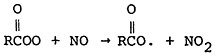
(23)
(24)
The first reaction, (23), converts NO to NO2 and claims the major portion of the peroxyl acyl radical. As soon as the NO has been depleted however, the second reaction becomes important and PAN’s are formed. This is very similar to the reaction scheme for ozone.
LITERATURE CITED
Calvert, J.G. (1973) Interactions of air pollutants. Proceed. of the conf. on health effects of air pollution. National Academy of Sciences, 19–101. October 3–5.
Corn, M., R.W.Dunlap, L.A.Goldmuntz, and L.H.Rogers (1975) Photochemical oxidants: sources, sinks, and strategies. J. Air Poll. Con. Assoc., 25(1) 16–18.
Davis, D.D., G.Smith, and G.Klauber (1974) Trace gas analysis of power plant plumes via aircraft measurement: O3, NOx, and SO2 chemistry. Science 186:733–736.
EPA (1970) Air quality criteria for nitrogen oxides. AP-84.
Gordon, R.J. and R.J.Bryan (1973) Ammonium nitrate in airborne particles in Los Angeles. Environmental Science & Technology 7(7):645–647. July.
Levy, H. (1971) Normal atmosphere: large radical and formaldehyde concentrations predicted. Science 173 (3992):141–143. July 9.
Stephens, E.R. (1973) Photochemical formation of oxidants. Proc. of conf. on health effects of air poll. 465–487. October 3–5.
APPENDIX 14-B
MEASUREMENT OF AMBIENT LEVELS OF NO2
Ambient air concentrations of NO2 are not well known because of problems with the Federal Reference method of measurement which was employed prior to 1972. The reference method used to determine compliance with national air quality standards was the Jacobs-Hochheiser (J-H) method as modified for the National Air Surveillance Networks (NASN). This method, along with other NO2 measurement techniques, is summarized in Table App. 14-B1 (Saltzman 1973).
Jacobs-Hochheiser Method
Briefly, the Jacobs-Hochheiser (J-H) method involves bubbling ambient air through an aqueous solution for 24 hours. The nitrate ions formed in the reagent are treated to form an azo dye which is measured colorimetrically. The intensity of the absorbed light at a specific wave length is related to the integrated 24-hour NO2 concentration. The collection efficiency of the reference method for NO2 was previously determined as 35 percent, and a correction for this efficiency had been applied to all data.
In 1971–72 it became apparent that the J-H method has two inherent problems which affected its ability to accurately estimate air quality in the field. These are: (1) the collection efficiency varies with concentration of NO2 and (2) a small portion of the nitric oxide (NO) in the ambient air shows up as NO2. The collection efficiency of the J-H method at NO2 concentrations in excess of 110 μg/m3 has been known for some time and calibration curves developed. These
TABLE App. 14-B1
Manual Methods Using Alkaline Absorbing Reagents
|
Name |
Reference |
Volume and Composition of Absorbing Reagent |
Absorbing Apparatus |
Sampling Rate and Time |
Procedure for Analysis |
Remarks |
|
Jacobs and Hochheiser (J-H) |
2 |
30–35 ml: 0.1N NaOH, 0.2% v/v butyl alcohol |
Coarse Fritted glass bubbler in sequential sampler |
1.3 lpm, 40 min. |
Add 1 drop 1% H2O2, 10 ml of 2% sulfanilamide in 5% v/v H3PO4; 1 ml of 0.1% N-(1-naphthyl)-ethylene diamine dehydrochloride |
No validation or stoichiometry studies. Data shows inverse relationship between SO2 and NO2 analyses, suggesting interference. 90% collected in first of two bubblers. |
|
Perry and Tabor (NASN) |
15, 16 |
20 ml: Same as J-H |
Polypropylene test tube containing glass inlet tube with orifice 0.36 ±0.05 mm. THERMOSTATED AT 35°C. |
0.15–0.20 lpm, 24 hrs. |
Autoanalyzer, using J-H reagents. |
Absorption in first of 4 bubblers varied from 30–69%. Collected samples stable for 3 weeks. Assumed 50% overall conversion. Large mass of data available using this method. |
|
Meadows and Stalker (Alabama Study) |
14 |
35 ml: 0.1N NaOH (in each of 2 bubblers) |
Two NASN bubblers in series. |
0.35–0.50 lpm, 24 hrs. |
Same as NASN. |
Absorption in 1st of 6 bubblers was 19%, in 1st 2 was 30%. Overall conversion of 36% used, with assumption of 100% stoichiometry. |
|
Federal Reference Method |
1 |
50 ml: 0.1N NaOH |
Membrane filter leading to polypropylene test tube with fritted glass inlet of porosity B (70–100 μm max. pore diameter). |
0.20 lpm, 24 hrs. |
Similar to J-H. |
Overall conversion of 35% is used. |
|
Name |
Reference |
Volume and Composition of Absorbing Reagent |
Absorbing Apparatus |
Sampling Rate and Time |
Procedure for Analysis |
Remarks |
|
Christie, et al. |
17 |
5 ml: 0.025 N NaOH, 0.1% NaAsO2, 0.75% sulfanilic acid |
Glass bubbler with open tube inlet. |
0.12 lpm, 1 min. |
Add 3 ml of 0.02% N-(1 naphthyl)-ethylene diamine dihydrochloride, 6% oxalic acid. |
Overall conversion 94% at 6 ppm NO2. For industrial hygiene use. |
|
Nash |
18 |
4 ml: 0.1N NaOH, 0.05% guaiacol (2-methoxy phenol) |
Glass Arnold Tube (with open tube inlet) |
0.6 lpm, 2 hrs. |
Add 4 ml of 0.2N HCl 0.5% sulfanilic acid, 1.5% glycine, 0.002% N-(1-naphthyl)-ethylene diamine dihydrochloride |
Limited amount of H2O2 may be added to reduce SO2 interference. Stoichiometric factor 0.73, absorption efficiency 99%. |
|
Huygen and Steerman |
19 |
15 ml: 0.1N NaOH, 0.02% R-salt (2-naphthol-3, 6-disulfonic acid disodium salt), 0.1% triethanolamine (in each of two bubblers). |
Two bubblers in series, each with coarse glass frit (90–150 μm) of 6.5 cm2 area. |
1 lpm, 24 hrs. |
Add to each absorber 15 ml of 0.4% sulfanilamide, 0.03% Cleves acid (8-aminonaphthl-2-sulfonic acid), 0.12N HCl. A drop of H2O2 may be added first to eliminate SO2 interference. |
Stoichiometric factor varied from 96% to 80% in range 48–2200 μg/m3 NO2. Absorption efficiency averaged 96%. |
|
EPA Tentative Candidate Arsenite Method |
6 |
50 ml: 0.1N NaOH, 0.1% sodium arsenite |
Polypropylene tube containing glass inlet tube with orifice 0.6±0.2 mm i.d., 6 mm from bottom of tube. |
0.2 lpm, 24 hrs. |
To 10 ml of absorbing solution, add 1 ml 0.024% H2O2; 10 ml of 2% sulfanilamide, 5% v/v H3PO4; and 1.4 ml of N-(1-naphthyl) -ethylene diamine dihydrochloride. |
Overall conversion is 85% over range 50–750 μg/m3 NO2 concentration. |
|
Levaggi, Siu, and Feldstein (triethanolamine) |
20 |
50 ml: 1.5% triothanolamine, 0.3% v/v n-butanol. |
Polypropylene tube with fritted glass inlet of 70–100 μm max. pore diameter. |
0.15–0.20 lpm, 24 hrs. |
Similar to J-H. |
Overall conversion efficiency 76–92% over range 56–750 μg/m3 NO2, collection efficiency 95–99%. Constant 0.85 factor recommended. |
show an approximate 35 percent collection efficiency at NO2 concentrations of 110 to 180 μg/m3. This means that about one-third of the NO2 in the air that bubbles through the sampler is trapped and bubbles through the sampler is trapped and analyzed. Late in 1971 lab methods became available to generate reliable low level NO2 concentrations and it was possible to extend the calibration curve for NO2 concentrations below 100 μg/m3. The extended curve showed that collection efficiencies greatly increased as NO2 concentrations decreased below 100 μg/m3. For example, at 100 μg/m3 the collection efficiency is just below 40 percent, whereas at 30 μg/m3 the collection efficiency is 60 percent. This variable collection efficiency may have been a major source of error in the observations used for classifying regions for NO2.
The J-H method as published in the Federal Register uses a constant average correction factor on a collection efficiency of 35 percent based on the early efficiency curves. It is clear (see Figure App. 14-B1) that a 35 percent collection efficiency is too low for concentrations in the 30 to 60 μg/m3 range. Therefore, at lower concentrations where collection efficiencies are much higher than 35 percent, the calculated and reported concentrations of NO2 obtained by the J-H method are higher than actual ambient NO2 concentrations. Since the NO2 concentration in the air varies throughout the day, the collection efficiency may vary significantly throughout any one 24-hour sample, making accurate calculation of NO2 concentrations impossible.
The NO interference previously mentioned is a second factor leading to an additive effect and is particularly important in areas of low NO2 concentrations. Table B2, The Effect of NO on the Reference Method for NO2, displays this additive interference of NO (Hauser and Shy 1972).
Because of the questionable data base, EPA reviewed all 47 AQCR’s in 29 states that were classified as Priority I for NO2 control and thus required stationary source controls. In July 1973, 43 of the original Priority I AQCR’s were reclassified as Priority III for NO2. The Los Angeles and Chicago AQCR’s are the only ones
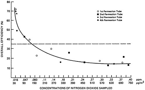
TABLE App. 14-B2
Effect of NO on the Reference Method for NO2
|
μg/m3 |
Ratio NO/NO: |
Expected NO: recovered, % |
Apparent NO: recovered, % |
|
|
NO2 |
NO |
|||
|
100 |
0 |
0.0 |
39 |
38 |
|
102 |
63 |
0.6 |
39 |
38 |
|
105 |
127 |
1.2 |
38 |
52 |
|
122 |
627 |
5.1 |
36 |
57 |
|
189 |
0 |
0.0 |
29 |
29 |
|
244 |
1205 |
4.9 |
24 |
45 |
|
248 |
1279 |
5.2 |
23 |
55 |
|
215 |
1242 |
5.8 |
26 |
50 |
|
311 |
0 |
0.0 |
20 |
17 |
|
316 |
111 |
0.4 |
20 |
30 |
|
318 |
332 |
1.1 |
20 |
33 |
|
356 |
1060 |
3.0 |
18 |
44 |
where the data indicated NO2 concentrations exceeding 110 μg/m3 annual average. Both of these AQCR’s remain Priority I. In the New York-New Jersey-Connecticut, Wasatch Front (Salt Lake City) and Denver AQCR’s (originally Priority III) arsenite data shows concentrations below the cutoff point for a Priority III classification, but chemiluminescence and/or Saltzman data show concentrations above it.
For more complete details of comparative sampling data performed in the original 47 Priority I AQCR’s, refer to Federal Register 38 FR 15181 (Federal Register 1973).
Proposed Reference Methods
Three methods of ambient NO2 monitoring have been proposed as the Federal Reference method: the modified sodium arsenite method, the continuous Saltzman method and the chemiluminescence detection method.
Each method has its own inherent limitations of either interferences, stability, complexity, toxicity, or cost. Each of the methods is briefly described.
Arsenite Method
Figure App. 14-B2 (Federal Register 1973) displays the apparatus used to determine NO2 (24-hour sample) by the Arsenite Method. Air is bubbled through a reagent of sodium hydroxide-sodium arsenite solution to form a stable solution of sodium nitrite (Christie et al. 1970). The nitrite ion produced during sampling is reacted with phosphoric acid, sulfanilamide, and N-1-naphthylethylenediamine dihydrochloride to form an azo dye. NO2 concentrations are infered by measuring the azo dye colorimetrically.
The method has an overall conversion efficiency of 85 percent over the range of 50–750 μg/m3 NO2. However, it has been reported that there is a 12 percent positive interference for NO which can be deducted (Saltzman 1973). The toxicity of the absorbing reagent is an obvious disadvantage of this method.
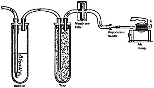
Continuous Saltzman Method
The principles of this method have been used for ambient air sampling for over 14 years (Saltzman 1960, Lyshkow 1965). By contacting an air flow with a liquid diazotizing-coupling reagent, the ![]() (nitrite ions) form a deeply colored azo dye which is measured colorimetrically. The absorbance of the azo dye is directly proportional to the number of NO2 molecules in the air stream that are converted to
(nitrite ions) form a deeply colored azo dye which is measured colorimetrically. The absorbance of the azo dye is directly proportional to the number of NO2 molecules in the air stream that are converted to ![]() .
.
This continuous method is applicable for concentrations from 18.8 μg/m3 to 1880 μg/m3 (.01–1 ppm). Apparently there is some interference from ozone. This is a negative interference reported as 5.5 percent for NO3/NO2=1, 19 percent for O3/NO2=2 and 32 percent for O3/NO2=3 (Federal Register 1973).
This method has the drawback of requiring considerable skill and effort for calibration and maintenance, especially replacement of the liquid reagent.
Chemiluminescence Method
The chemiluminescence instrument represents a major break with absorbing wet chemistry methods of ambient air sampling. Figure App. 14-B3 schematically illustrates the NOx chemiluminescent analyzer (Federal Register 1973). In general, the analyzer draws an air sample into a light-tight reaction chamber and mixed with ozonated air. The chemiluminescence produced by the reaction of nitric oxide is measured by a photomultiplier tube, and the data is stored in a peak-holding amplifier.
The first generation chemiluminescence instruments alternately sampled NO and total NOx. The total NOx was determined by converting all NO2 to NO and measuring as described above. The difference between total NOx and NO was taken as NO2. This 1-minute cycling of samples often gave negative NO2 values when NO concentrations were high and rapidly varying, such as near traffic. The latest analyzers operate
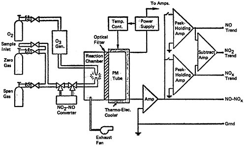
with dual chambers or a rapidly cycling single chamber. This improvement has apparently removed spurious negative values.
Since the instrument measures the light emissions of individual molecules, its lower detectable values are dependent on photomultiplier sensitivity. The lower limit of this method is approximately 9.4 μg/m3 (0.005 ppm).
The direct measurement of NO has no interferences. However, the conversion of NOx to NO by the converter can decompose unstable nitrogen compounds to give a falsely high NOx reading. Fortunately interference is small (Federal Register 1973).
Selection of a New Federal Reference Method
An extensive field study is now being conducted by EPA to determine the proper priority classifications of numerous air quality control regions. The arithmetic average results for 42 regions by simultaneous analysis with the Tentative Candidate Chemiluminescent Method and the Tentative Candidate Arsenite Method have been tabulated in 38 FR 15174. Figure App. 14-B4 shows a plot derived from these data by Saltzman. Even though the methods were selected as best, after much testing, there is a disturbing scatter in the comparison plot. The straight line fit by the method of least squares has the equation:
The diffuculty and expense of validating analytical methodology has been grossly underestimated in the past.
Calibration Techniques
Standardized calibration techniques are essential to all ambient air quality monitoring. Precise procedures for calibration of each of the tentative NO2 methods are given in 38 FR 15174. There are two techniques described:
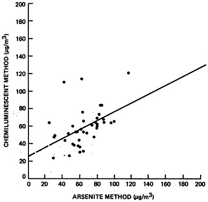
NO2 permeation tube and dilution, and NO2 gas-phase titration.
The latter, gas-phase titration, is diagrammed in Figure App. 14-B5 (Federal Register 1973). This apparatus can calibrate chemiluminescent NO, NO2, and O3 instruments.
LITERATURE CITED
Christie, A.A., R.G.Lidzey, and D.W.F.Radford (1970) Analyst 95, 519.
Federal Register (1973) 38(110), 15174–15191 June 8.
Hauser, T.R., and C.M.Shy (1972) Position paper: NOx measurement env. res. and tech. 6(10), October.
Lyshkow, N.A. (1965) A rapid sensitive colorimetric reagent for nitrogen dioxide in air. J. Air Poll. Cont. Assoc. 15(10):481.
Saltzman, B.E. (1973) Analytical methodologies for nitrogen oxides in perspective. Proceed of the conf. on health effects of air pollution. National Academy of Sciences, Washington, D.C. October 3–5.
Saltzman, B.E. (1960) Modified nitrogen dioxide reagent for recording air analyses. Anal. Chem. 32, 135.

APPENDIX 14-C
PROJECTIONS OF FUTURE NOx EMISSIONS
TOTAL EMISSIONS: 1972–1990
Total emissions of nitrogen oxides projected to 1990 assuming implementation of the present statutory program for NOx control are displayed in Table App. 14-C1 and Figure 14–16 in Chapter 14. This estimate projects a 36 percent increase in total emissions from 1972–1990. The largest increases in emissions will be produced by industrial process losses (98 percent), non-highway transportation (72 percent), industrial fuel combustion (54 percent) and electric power generation (49 percent). Highway-related transportation emissions will decline by 24 percent during this period assuming the statutory emission standards for automobiles are achieved. The estimate is considered to be conservative since it assumes that (1) most new electric power generation will be produced by nuclear reactors, (2) the statutory automotive emission standards will remain in effect and be achieved and (3) the 1940–1970 annual growth rate of NOx emissions from industrial, commercial and institutional fuel combustion will slow during the next two decades.
Emission projections for electric power generation are based on recent electric generation forecasts by the Federal Energy Administration (USEPA 1975) and the National Academy of Engineering (NAE 1974). These projections are discussed in greater detail below.
Industrial fuel combustion emissions of nitrogen oxides grew at the rate of 9.5 percent per year during the 1960–1972 period due to a
TABLE App. 14-C1
Nationwide NOx Emissions Projected to 1990 Assuming the Present Statutory Program
|
|
NOx Emissions (106 tons/year) |
|||
|
Source Category |
1972 |
1980 |
1985 |
1990 |
|
Stationary Fuel Combustion |
12.27 |
15.96 |
16.82 |
18.46 |
|
Electric Generation |
5.94 |
8.16 |
8.20 |
8.88 |
|
Industrial |
5.39 |
6.73 |
7.46 |
8.31 |
|
Commercial-Institutional |
0.65 |
0.76 |
0.84 |
0.93 |
|
Residential |
0.29 |
0.31 |
0.32 |
0.34 |
|
Industrial Process Losses |
2.88 |
3.91 |
4.72 |
5.71 |
|
Solid Waste Disposal |
0.18 |
0.22 |
0.25 |
0.28 |
|
Transportationa |
8.45 |
8.47 |
7.49 |
7.60 |
|
Road Vehicles |
7.48 |
7.14 |
5.89 |
5.68 |
|
Gasoline |
6.59 |
5.97 |
4.30 |
3.95 |
|
Diesel |
0.89 |
1.17 |
1.59 |
1.73 |
|
Other |
0.97 |
1.33 |
1.60 |
1.92 |
|
Miscellaneousb |
0.59 |
0.74 |
0.87 |
1.02 |
|
TOTAL |
24.37c |
29.30 |
30.15 |
33.07 |
|
aAssumes a 4% annual VMT growth rate bIncludes New York City Point sources assumed to grow at 4% per year c1972 total emissions are 270,000 tons lower than those summarized in Table 2.2 due to the use of new road vehicle emission factors |
||||
large increase in natural gas and industrial process gas combustion. In this projection it is assumed that the growth rate will slow to approximately 2.5 percent per year through 1990 due (1) to a gradual shift to purchase of electricity from utility companies, and (2) to an assumed 3 percent annual growth rate in use of natural and industrial process gas, and in the use of coal. A 3 percent growth rate for industrial process gas use follows the growth rate for steel and petroleum production. No increase in oil consumption is assumed after 1975. Since there are no federal new source performance standards and few state regulations for NOx emissions from medium-sized and small boilers, all emissions are uncontrolled. Because historical trends show a much larger growth rate than as sumed here, these projections are considered conservative.
NOx emissions from commercial and institutional fuel combustion have grown at the rate of 4.5 percent per year over the last three decades. In this projection it is assumed that the growth rate will slow to approximately 2 percent per year through 1990 due to (1) a gradual shift to the purchase of power for space heating and electricity from utility companies, and (2) energy conservation measures. No controls were assumed for industrial fuel combustion sources. These projections are also quite conservative since they depart significantly from historical trends.
Residential fuel combustion emissions of NOx have declined at the rate of 2 percent per year over the last three decades. This is primarily due to a shift in fuel usage from coal to distillate oil and natural gas and to the purchase of power for space heating from electric utilities. In this projection it is assumed that residential emissions will grow 1 percent per year through 1990 since: (1) the benefits of a coal to oil or natural gas shift will all have been realized by 1975; (2) the number of housing units increase at a rate of 2 percent per year; and (3) approximately half of the new housing units will be heated by electricity.
Lack of knowledge of NOx emission factors from industrial process losses in the past make
historical trends for these sources difficult to interpret. It is assumed that refinery emissions which amount to 86 percent of all industrial process loss emissions, will increase at the rate of 4 percent per year, which is the growth rate for petroleum usage. Since there are no federal new source performance standards for NOx from refineries it is assumed that these sources will be uncontrolled. Nitric acid manufacturing emissions of NOx are assumed to grow at 2.6 percent per year which reflects the mix of old and new sources and the 90 percent control of emissions from new sources required by federal new source performance standards. These emission estimates are conservative since baseline 1972 petroleum refinery emissions are probably underestimated.
NOx emissions from solid waste disposal grew at a rate of 4 percent per year from 1940–1970 due to open burning and incineration. State implementation plans required by the Clean Air Act will eliminate most of the open burning emissions so that it is more realistic to assume only a 1 percent annual growth rate of such emissions through 1990. The scarcity of land for sanitary landfill, and the increase in per capita solid waste production will probably result in at least a 5 percent annual growth rate in incineration emissions. Overall, it is assumed that solid waste emissions will grow at a rate of 2.6 percent per year.
Non-highway transportation sources grew at the rate of 5 percent per year from 1940–1960 and 12.5 percent per year from 1960–1970. As reliance on petroleum products decreases with energy conservation measures, this projection assumes that the growth rate will slow to 4 percent per year through 1980 and 3.8 percent per year from 1980–1590. The slower increase in the 1980–1990 period is due to the effect of new aircraft emission standards effective on 1979 and later model year aircraft engines. Again, it is likely that the estimates are conservative since they depart significantly from historical trends.
ELECTRIC POWER GENERATION EMISSIONS: 1972–1990
Emission projections for electric power generation were based on recent electric generation forecasts by the Federal Energy Administration (USEPA 1975) and the National Academy of Engineering (NAE 1974). These forecasts include generating capacity and actual power output for 1980 and generating capacity projections for 1985. Actual power output for 1985 and both generating capacity and actual power output for 1990 were projected from 1972–1980 data which indicates a 6.5 percent annual increase in power usage. The ratio of actual power output to generating capacity, i.e., load factor, was assumed to remain constant from 1980 to 1990 for each power source. The projections of generating capacity, actual power output and emissions are summarized in Table App. 14-C2.
As seen in Table App. 14-C2, nuclear power generation will increase significantly from 1972–1990 under the assumptions of Project Independence. Coal generation will also increase and natural gas generation will decrease by 10 percent during that same period. All new coal, oil and natural gas generation is assumed to meet federal new source performance standards for NOx emissions. One-quarter of the existing plants are assumed to be retired and replaced by new facilities every 5 years. Resulting emissions from electric power generation will increase 49 percent from 1972–1990 due to the increase in emissions from coal fired plants.
These emission estimates reflect the projected predominance of nuclear power in electric generation. If for some reason a decision should be made not to build any new nuclear power plants after 1975, quite a different picture would emerge. As can be seen in Table App. 14-C3 and Figure App. 14-C1, such a policy decision would result in nearly a doubling of NOx emissions in 1990 if coal fired plants provided the capacity that was projected for nuclear power. If the projected growth of nuclear generation were slowed rather than halted then the resulting NOx emissions would fall somewhere between the projected extremes displayed in Table App. 14-C3 and Figure App. 14-C1.
TABLE App. 14-C2
NOx Emission Projections to 1990 from Electric Power Generation Assuming Project Independence
|
Energy Source |
Gen. Cap. (MW) |
Power Output (109 kwh) |
Emissions (106 tons) |
Gen. Cap. (MW) |
Power Output (109 kwh) |
Emissions (106 tons) |
Gen. Cap. (MW) |
Power Output (109 kwh) |
Emissions (106 tons) |
|
|
1980 |
1985 |
1990 |
||||||
|
Coal |
295,000 |
1608 |
7.21 |
330,000 |
1734 |
7.21 |
402,000 |
1972 |
7.89 |
|
Oil |
59,000 |
165 |
0.52 |
52,000 |
146 |
0.52 |
52,000 |
146 |
0.52 |
|
Natural gas |
86,000 |
145 |
0.48 |
78,000 |
178 |
0.44 |
78,000 |
178 |
0.44 |
|
Gas Turbine |
61,000 |
53 |
0.03 |
61,000 |
53 |
0.03 |
61,000 |
53 |
0.03 |
|
Hydroelectric |
88,000 |
325 |
- |
75,000 |
276 |
- |
75,000 |
276 |
- |
|
Nuclear |
73,000 |
394 |
- |
250,000 |
1314 |
- |
500,000 |
2,452 |
- |
|
Other |
- |
- |
- |
61,000 |
53 |
- |
75,000 |
66 |
- |
|
Total |
662,000 |
2,740 |
8.16 |
907,000 |
3,754 |
8.20 |
1,243,000 |
5,143 |
8.88 |
TABLE App. 14-C3
Nationwide Emissions of NOx from Electric Power Generation Projected to 1990 for Two Policy Options
|
|
NOx Emissions (106 tons/year) |
|||||||
|
YEAR |
Project Independence |
No New Nuclear Plants Built After 1975 |
||||||
|
Totala |
Coal |
Oil |
Natural Gas |
Totala |
Coal |
Oil |
Natural Gas |
|
|
1972 |
5.94 |
3.95 |
0.85 |
1.14 |
5.94 |
3.95 |
0.85 |
1.14 |
|
1980 |
8.24 |
7.21 |
0.52 |
0.48 |
9.32 |
8.29 |
0.52 |
0.48 |
|
1985 |
8.20 |
7.21 |
0.52 |
0.44 |
12.81 |
11.82 |
0.52 |
0.44 |
|
1990 |
8.88 |
7.89 |
0.52 |
0.44 |
17.56 |
16.57 |
0.52 |
0.44 |
|
aTotal contains 0.03×10⁶ tons/year from gas turbines |
||||||||
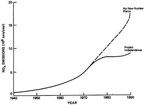
ROAD VEHICLE PROJECTIONS
Past highway statistics (FHA 1972) on vehicle-miles-of-travel (VMT) are used to project NOx emissions to 1990 for road vehicles including light-duty passenger vehicles, light and heavy duty gasoline trucks and heavy duty diesel trucks and buses. Three options for control are considered: (1) no controls on NOx emissions with the statutory program for CO and HC in effect; (2) a 5 year delay of the 1977 statutory standards, i.e., maintenance of the interim standard for NOx emissions of 2 g/mile until 1983; and (3) the present statutory program (NOx emissions of 0.4 g/mile by 1977). Two different VMT growth rates are considered: (1) 2 percent annual increase and (2) 4 percent annual increase. The former assumes stringent gas conservation measures while the latter assumes no restraint. The resulting projections are displayed in Table App. 14-C4 and Figure App. 14-C2.
The present statutory program will result in a 25 percent reduction in 1972 road vehicle emissions by 1990 for a VMT growth rate of 4 percent. A 5 year delay of the 1977 automotive standards will result in only a 17 percent reduction in 1972 emissions by 1990 for the same VMT growth rate. In addition to growth in total VMT, growth in uncontrolled heavy duty gasoline and diesel truck usage will be responsible for the fact that emission reductions predicted in 1990 are considerably smaller than the percentate reduction in emissions per mile required by the standards for light-duty automobiles. These heavy duty sources become major contributors to total transportation emissions during the 1980’s.
TABLE App. 14-C4
Nationwide NOx Emissions From Road Vehicles Projected to 1990 for Three Policy Options
|
|
NOx Emissions (106 tons) |
|||||
|
2% Annual Growth in VMT |
4% Annual Growth in VMT |
|||||
|
YEAR |
No Control |
Present Statutory Program |
Proposed 5-year Standards Delaya |
No Control |
Present Statutory Program |
Proposed 5-year Standards Delaya |
|
1972 |
7.62 |
7.48 |
7.48 |
7.62 |
7.48 |
7.48 |
|
1975 |
8.55 |
7.82 |
7.82 |
9.08 |
8.31 |
8.31 |
|
1980 |
9.49 |
61.4 |
7.37 |
11.06 |
7.14 |
8.60 |
|
1985 |
10.35 |
4.44 |
5.60 |
13.48 |
5.89 |
7.38 |
|
1990 |
11.22 |
4.03 |
4.38 |
15.86 |
5.68 |
6.18 |
|
a1977 auto emission standards for NOx postponed until the 1982 model year. California interim standard of 2.0 g/mi applies to 1977–1982 model years. |
||||||
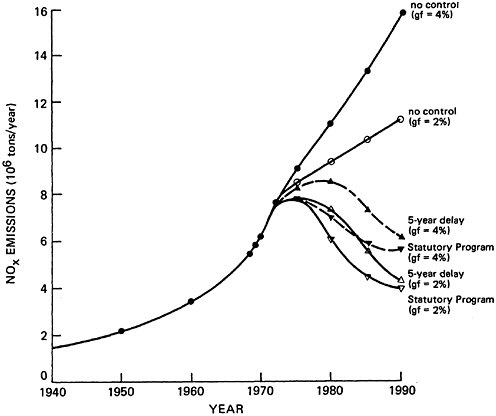
LITERATURE CITED
Federal Highway Administration 1972, “Highway Statistics,” Office of Highway Planning.
National Academy of Engineering 1974b, “U.S. Energy Prospects: An Engineering Viewpoint,” Task Force on Energy.
U.S. Environmental Protection Agency 1975, “Federal Energy Administration Electric Generation Projections,” Personal Communication with James Speyer, Office of Planning and Management.
CHAPTER 15
NITROGEN OXIDE CONTROL TECHNIQUES
OVERVIEW
This chapter makes substantial use of reports and information made available by a large number of government and private institutions. Special thanks are due to the Combustion Research Section of the EPA Control System Division.
Throughout this section, emissions have been converted to lbs/106 BTU expressed as NO2 in order to facilitate comparison of emissions from different sources. A table of conversion factors appears in Appendix 15-A.
Typically, nitrogen oxides are formed in localized, high-temperature regions in combustors by the oxidation of both atmospheric nitrogen (thermal NOx) and nitrogen that may be contained in the fuel (fuel NOx). The formation of NOx in combustion systems can be suppressed, with varying degrees of success, by reducing the oxygen content and the temperature in the localized regions in the combustor contributing to emissions, usually in the vicinity of the flame. Reductions in the oxygen content in the flame zone reduce the emissions of both fuel and thermal NOx; reductions in temperature, however, produce significant reductions in only the thermal NOx.
Injection of cooled combustion products, steam, or water into the flame volume; reduction of temperature to which combustion air is
preheated; and extraction of heat from the flame volume are methods that have been used to reduce the temperature in the combustor. The injection of cooled combustion products into the flame volume can be achieved externally by ducting relatively cool combustion products to the burner area (referred to as flue gas recycle for furnaces or exhaust gas recycle for engines) or internally by modifying the burner design so as to induce the entrainment of colder combustion products by the hot gases leaving a burner.
Methods for reducing the oxygen content in the flame zone involve lowering the volume of air supplied to the burners by reducing the overall air/fuel ratio to the combustor (referred to as low-excess-air firing) or by reducing the air/fuel ratio for some burners without reducing the overall air/fuel ratio (referred to as staged combustion).
Low excess-air firing can achieve modest reductions in NOx emissions. However, its application is limited by the ability to reduce the air/fuel ratio to burners without producing excessive emissions of carbon monoxide and particulates.
There are several variations on staged combustion, referred to as biased firing, off-stoichiometric firing, overfire air and two-stage combustion. In general, the air/fuel ratio to some or all of the burners is reduced, to as low as seventy percent of the value required for combustion. The combustion is then completed by the addition of the balance of the air requirement after an interval in which the combustion product is allowed to partially cool. In engines a form of staged combustion is achieved by stratifying the fuel charge to provide local regions of relatively high fuel concentration, facilitating combustion at overall air/fuel ratios considerably higher than those practical for a uniform charge.
Many of the results reported in this chapter are from tests performed in laboratories or on small-scale units. Some of the results point to promising techniques or methods for nitrogen oxide emission control. However, it should be borne in mind that the application of test results
to large scale, operational systems often introduces significant problems, many of which are indicated throughout the chapter. The success of a test does not necessarily imply easy transfer to a large, commercially practicable system and considerable effort is being, and will continue to be, directed toward the resolution of the problems which arise when such a transfer is attempted.
Utility boilers and gas turbine engines have received priority in the development of nitrogen oxide emission control technology. Other major sources, particularly stationary reciprocating engines, have received relatively little attention.
Utility Boilers
As noted in Chapter 14, utility boilers fired by coal, gas, and oil accounted for nearly half of the stationary emissions of NOx in 1972. Based upon a field test performed by Esso Research and Engineering and other data, EPA has developed emission factors which indicate that NOx emission rates for existing boilers range from 0.6 to 1.2 lbs/106 BTU for coal-fired units, from .27 to .7 lbs/106 BTU for oil-fired units, and from .12 to .7 lbs/106 BTU for tangentially fired boilers using gas. The lowest emissions were from tangentially-fired units and the highest from units with intense combustion. Emissions decreased substantially with decreased furnace load.
Low-excess-air firing, staged combustion, flue-gas recirculation, water injection and reduced air preheat are control techniques that have been successfully demonstrated on field units. The latter two methods, however, have an associated and usually unacceptable penalty in thermal efficiency of the boiler. Flue gas recirculation is most effective for gas-fired units but is relatively uneffective for oil-fired and coal-fired units in which the fuel NOx contribution is significant. By the utilization of a combination of control techniques an average reduction in emissions of 60 percent has been achieved for gas-fired units, 48 percent for oil,
and 37 percent for coal. In the case of coal, the locally fuel rich conditions may contribute to slagging or corrosion problems. Accelerated corrosion testing over 300 hours showed no adverse effects but longer range trials for a wide range of coals are needed before the control techniques can be commercially accepted.
The applicability of combustion process modification to existing furnaces must be evaluated on a case-by-case basis. Boilers can generally be adapted for low-excess-air firing and staged combustion without major modification. Flue-gas recirculation, however, may be impractical for retrofitting except on units which have had the ducting already installed for steam temperature control. The capital costs vary widely with specific installation size and design; they range from under $0.50/KW for staged combustion to $6.0/KW for flue gas recirculation on existing units and from negligible costs for staged combustion to $4.0/KW for flue gas recirculation on new units.
Equipment manufacturers can meet existing emission standards on new units but usually specify an upper limit on the nitrogen content of the fuel oils that can be burned without exceeding the standards. EPA has proposed emission levels that might be achieved in the future: 0.12 lb/106 BTU (100 ppm) for gas, 0.20 lb/106 BTU (150 ppm) for oil, and 0.28 lb/106 BTU (200 ppm) for coal by 1980; and 0.06 lb/106 BTU (50 ppm) for gas, 0.12 lb/106 BTU (90 ppm) for oil, and 0.14 lb/106 BTU (100 ppm) for coal by 1985. These are technological goals that can probably be met on individual units if adequate research is carried out on new control techniques, pilot-plant development and field-demonstration. It should be recognized that high-intensity combustion burners may be required to burn certain types of coals, and these will yield higher emissions than the projected goals. Further, there is a significant lag time between the development of new designs and installation of field-units by the utilities.
Industrial Boilers
Most boilers with 10 to 500 million BTU/hr
capacity can meet the new source performance standards for units greater than 250 million BTU/hr capacity with only minor modifications in operating conditions. Still lower emission levels are possible, but redesign of the boilers would be required to allow off-stoichiometric or staged-combustion in units burning heavy fuel oils or coal since very few existing units possess the necessary flexibility. Problems which must be considered in the design of new units, and particularly in the modification of existing units, include corrosion and deposits on boiler tubes, flame instability, and combustion noise. The level of control that is achievable on industrial boilers is close to but not as great as that attainable with utility boilers.
Commercial and Residential Space Heating
Small space heating equipment (less than 10 million BTU/hr) fueled with natural gas or distillate oil generally has the lowest specific NOx emissions of any class of combustion equipment (i.e., 0.05 to 0.20 lb NO2/106 BTU) and produces about seven percent of the stationary source NOx. Existing units have little flexibility for NOx control, and the emissions are unaffected by normal maintenance operations. Combustion improving devices generally increase NOx emissions by producing a more intense flame region, but optimized burners, based either on conventional designs or on new combustion concepts such as catalytic combustion, which emit from 0.015 to 0.05 lb NO2/106 BTU have been demonstrated in tests.
Stationary Engines
About 18.8 percent of the stationary source NOx is produced by reciprocating engines. Spark-ignition gas engines produce about 63 percent of the engine NOx, primarily in applications associated with the gas industry, i.e., pipelines and natural gas production and processing.
Moderate reduction in NOx emissions from these engines (20 to 40%) can be achieved, while reducing fuel consumption, by cooling the fuel/ air mixture. Further reductions in NOx emissions from existing, engines are possible, but have generally been accompanied by a significant increase in fuel consumption. New engine designs, such as those using stratified charge concepts, may produce substantial reductions in NOx without increasing fuel consumption; however, further development work is required.
Diesel engines produce about 34 percent of the engine NOx in agricultural and industrial applications. As in spark ignition engines, cooling the intake air, can reduce NOx emissions while decreasing the fuel consumption. Water injection can also reduce NOx emissions with little change in fuel consumption; however, corrosion may be a problem, particularly if the engine is used on a standby basis. NOx emissions have been reduced by as much as 50 percent with little penalty in fuel consumption, but lower emission levels may require substantial engine redesign, e.g., prechamber engines; or exhaust gas treatment using catalytic reduction of NO to N2; or may result in significant increases in fuel consumption. EPA projects that emission levels of 0.14 lb, NO2/106 BTU for spark ignition gas engines and 0.16 lb NO2/106 BTU for diesel engines may be reasonably achieved by 1980, but there may be some increase in fuel consumption.
Stationary gas turbine NOx emissions can be reduced to the levels of currently proposed emission standards through the use of steam or water injection into the combustion chamber. Further reductions are possible through combuster design modifications including use of out-of-line combustion chambers; improved fuel atomization and mixing; prevaporized, premixed combustion; internal recirculation of combustion products; and surface combustion. The use of heavy fuel oils, rather than natural gas or distillate oils, will probably result in higher emission levels due to fuel nitrogen and may require new measures to control NOx.
The efficiency of gas turbines varies from 24 percent for simple cycle gas turbines to more
than 40 percent for combined gas turbine—steam turbine cycles. Emission standards based upon thermal input (e.g., lb.NOx/106 BTU or ppm NOx at 15 percent oxygen) provide no credit for higher efficiencies and, in fact, may inhibit the development of more efficient systems.
Fluidized Bed Combustion
Fluidized bed combustion of coal provides a potential alternative to current utility boiler design that is competitive when a low-sulfur fuel or flue-gas treatment is required to meet the emission standards for sulfur oxides. Atmospheric pressure and pressurized combustors with dolomite injection for control of sulfur oxide emissions are at a pilot-plant stage. A demonstration of a 30 MW atmospheric pressure fluidized-bed combustor is scheduled for 1975 and it is projected that 200 MW and 800 MW units may be built as early as 1977 and 1980, respectively.
At the low temperatures of operation of fluidized bed combustors, typically 1500F to 1800F, most of the NOx is contributed by the oxidation of fuel nitrogen. Tests on laboratory and pilot-scale fluidized-bed combustors have yielded emissions that meet the current standards for new coal-fired units. Emissions as low as 0.11 lbs/106 BTU have been obtained without the benefit of staging. Tests on larger-scale units are needed to establish practical emission levels for commercial units.
Tall Stacks and Intermittent Control Strategies
The only intermittent control strategy that appears practical for NOx emission reduction is load switching of electric power generation. Load switching has limited applicability because of the variability in the contribution of electric power generation to local emissions. The advantages of tall stack release of sulfur dioxide to reduce ground level concentrations do not apply for NO. Tall stacks
potentially reduce ground level NO concentrations however, NO converts to nitric acid and nitrates faster than does SO2 to sulfuric acid and sulfates and since the reaction products precipate, there is a greater potential for local impact. There is considerable uncertainty about the effects of NOx release from tall stacks on the formation of photochemical oxidants and the ground level concentrations of oxidants and nitrogen dioxide.
Future Trends
A major shift from gas to coal is expected in fuel utilization for utility boilers, and to a lesser extent smaller combustors. Emissions would be expected to increase unless new levels of control are achievable for the combustion of coal. Shale and synthetic fuels from coal may have higher nitrogen contents than existing fuels and may yield high NOx emissions.
Although significant success has been achieved in reducing NOx emissions from stationary sources, the reductions that have been achieved, typically 50 percent, are much smaller than existing potential. New combustion systems, utilizing surface or catalytic combustion, have the potential to eliminate thermal NOx. Significant reduction in the emissions from coal-fired units have been achieved by burner modification on a pilot scale, and the potential exists of designing burners with emission levels for coal below 0.2 lb/106 BTU.
Flue gas treatment is more expensive than combustion process modification but at present can attain much higher reduction in NOx emissions. A number of flue gas treatment methods are at a pilot plant demonstration stage, primarily in Japan.
Institutional Constraints
The reduction of NOx from stationary sources is subject to a number of economic and logistic constraints. Capital availability may limit the
rate at which new, more expensive equipment with reduced NOx emissions can be brought on line and may severely constrain the rate at which existing equipment is brought into compliance with emission standards by retrofit. Increased operating costs due to new maintenance requirements, increased fuel consumption, decreased capacity, or increased labor to provide the closer control of combustion conditions required for NOx control must also be factored into the decision making process.
Equipment outages for modification of existing facilities present an additional constraint, particularly in the electric utilities. Some modifications may be prepared in advance and installed during scheduled outages; however, prolonged outages, which may be required for the modification of some units, may strain the system generating capacity and will, therefore, require careful scheduling in order to permit utilities to meet demand. The logistics of modifying a very large number of units of diverse types may inhibit the retrofit of smaller sources.
NOx control techniques have been developed for those applications for which emission regulations have been proposed (e.g., utility boilers and stationary gas turbines) providing an economic incentive for equipment manufacturers to develop NOx controls. Where funding has been available for research on NOx control, significant progress has been made toward developing control techniques. On the other hand, there is little incentive to develop burners or small package boilers with low-NOx emissions, so progress in development is slow for these systems. Reduction of NOx emissions from systems for which development incentives do not exist, (e.g., industrial process furnaces) has received little attention.
INTRODUCTION
Stationary Sources of Nitrogen Oxides
Stationary sources currently contribute more than half of the man-made emissions of NOx in the U.S. The NOx emissions are dominated by combustion sources burning coal, gas, and oil (Mason and Shimzu 1974). The major sources are utility boilers and stationary engines. Nitric acid and nitrogen fertilizer plants contribute a small fraction of the national total, although their emissions may be locally significant in some areas.
The nitrogen oxides emitted by combustion sources are predominantly in the form of nitric oxide (NO) with the residual, usually less than 5 percent, in the form of nitrogen dioxide (NO2). The oxides are formed either by the oxidation of atmospheric nitrogen at high temperatures (thermal NOx) or by the oxidation of nitrogen compounds in the fuel (fuel NOx). The relative contributions of thermal and fuel NOx depend on combustor design and operating conditions, as well as on the nitrogen content of the fuel. As much as half of the total stationary emissions may be contributed by the oxidation of the nitrogen in the fuel, primarily in units burning heavy-oils and coals.
Control Options
The technology for controlling the emission of nitrogen oxides from combustion sources is based on either the modification of the combustion process to prevent formation of the oxides or the treatment of the product gases to destroy or remove the oxides. The latter option is made difficult by the relative inertness and insolubility of NO; wherever combustion process modification has yielded the needed reduction in NOx emissions, it has proven to be the most economical method for doing so. In some cases, where stringent emission controls have been imposed on combustion sources, a combination of
combustion process modification and product gas treatment has been proposed (Tohata 1974). For NOx emissions from chemical plants, a variety of control techniques are available, including catalytic destruction, afterburning, absorption and adsorption.
MECHANISMS FOR NITRIC OXIDE FORMATION
Thermal Fixation of Atmospheric Nitrogen
The formation of thermal NOx is determined by highly temperature dependent chemical reactions the so-called Zeldovich (1946) reactions. The rate of formation is significant only at high temperatures (greater than 3300F) and doubles for every increase in flame temperature of about 70F. The rate of formation increases with increasing oxygen concentration (rate proportional to the square root of the oxygen concentration) except in a small region near the flame zone in which superequilibrium concentrations of oxygen atoms are found (Thompson et al. 1972, Sarofim and Pohl 1973, Livesey et al. 1971). Although the NOx emitted by most practical combustors is predominantly in the form of NO, there is evidence from laboratory studies that a significant fraction of the NOx may be present as NO2 in localized regions of a flame (Merryman and Levy 1974).
Formation of Fuel NOx
An upper bound for the potential contribution of fuel-nitrogen to NOx formation may be gauged from the nitrogen content of fuels. Natural gas has negligible amounts of organically bound nitrogen, U.S. crude oils have nitrogen concentrations that average about 0.15 percent by weight (Martin and Berkau, Ball et al. 1951) and U.S. coals have nitrogen concentrations that average about 1.4 percent by weight. The nitrogen content in the crude oil varies between oil fields (Table 15–1), and is high for California oils. During the refining of oils, the nitrogen
TABLE 15–1
Nitrogen Content in U.S. Crude Oils in Million Barrels (Ball et al. 1951, Ball and Wenger 1958, Vandaveer 1965, Aga et al. 1973)
|
|
Proved Reserves (1972) |
Production (1972) |
Average Weight % Nitrogen |
||
|
MM bbl |
% |
MM bbl |
% |
|
|
|
Texas |
12,144 |
33.4 |
1,258 |
38.3 |
0.074 |
|
Alaska |
10,096 |
27.8 |
73 |
2.2 |
— |
|
Louisiana |
5,028 |
13.8 |
780 |
23.8 |
0.056 |
|
California |
3,554 |
9.8 |
346 |
10.5 |
0.49 |
|
Oklahoma |
1,303 |
3.6 |
198 |
6.0 |
0.151 |
|
Wyoming |
950 |
2.6 |
139 |
4.2 |
0.183 |
|
New Mexico |
582 |
1.6 |
106 |
3.2 |
0.082 |
|
U.S. Total |
36,339 |
92.6 |
3,231 |
88.2 |
— |
concentrates in the heavy fractions so that, residual oils from a California crude may have as much as 1.1 percent nitrogen whereas light distillate oils generally have nitrogen concentrations under 0.1 percent. The spread in nitrogen concentrations for coals is shown in Figure 15–1. The concentration is reported as lbs-NO2 per million BTU assuming 100 percent conversion of fuel nitrogen to NO2. Also shown on the plot are the sulfur concentrations, reported as lbs-SO2/106 BTU, and the percentage of U.S. coal reserves that have nitrogen and sulfur concentrations below certain levels. There is no apparent correlation between coal nitrogen content and coal sulfur content.
A fraction of the fuel nitrogen is converted to nitric oxide in practical combustors. Tests on carefully controlled laboratory-scale units have typically shown that 15 to 100 percent of the fuel nitrogen is converted to NOx (Figure 15–2), with the higher conversion efficiencies obtained when the nitrogen content is low or when the combustor is operated lean.
Because it is not easy to separate the contribution of fuel NOx from thermal NOx, the conversion efficiency of fuel nitrogen to NOx in large scale units is not known with certainty, but estimates obtained from field tests show trends similar to those obtained in the laboratory. A plot of the total uncontrolled NOx emissions from large and small scale units, Figure 15–3, suggests that the emissions increase with increases in fuel nitrogen content for units ranging in size from laboratory units to utility boilers. Emissions from large gas-fired units account for the high emission data at zero nitrogen content.
The mechanism by which the fuel nitrogen is converted to nitrogen oxides is imperfectly understood. The conversion efficiency of fuel nitrogen to NOx is found to increase markedly with increased oxidizing conditions in the flame but is insensitive to changes in temperature (Fenimore 1972, Martin and Berkau).
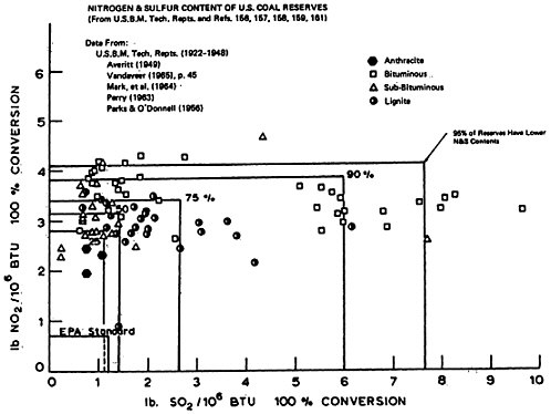
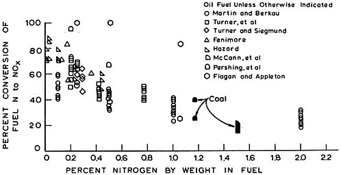
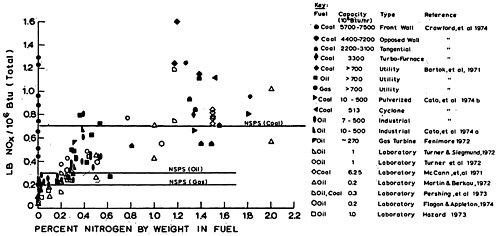
FACTORS INFLUENCING NOx EMISSIONS
The rate of formation of nitric oxide in flames by the two mechanisms discussed above is a sensitive function of oxygen content and, for thermal NOx, temperature. Any factor which influences temperature and oxygen concentration profiles in combustors may therefore have an influence on NOx emission. This makes generalizations for practical systems difficult since fuel/air ratios, fuel/air mixing patterns, fuel type, interaction of different burners, and placement of heat transfer surfaces all influence emissions. Additional complications are introduced by the fact that NO may be reduced by reactions with hydrocarbons in flames and that hydrocarbons can react with atmospheric nitrogen to form nitrogen-containing compounds that are in turn oxidized to nitric oxide. The following sections indicate some of the factors that influence emissions.
Air Preheat
Increased air preheat increases flame temperature and the contribution of thermal NOx. The increases observed in practice for premixed flames are in agreement with predictions from theory (Lange 1972). Reducing air preheat has been shown to decrease emissions on full-scale utility boilers (Blakeslee and Burbach 1972) but it carries with it an associated penalty in thermal efficiency.
On the other hand, in reciprocating engines reducing the inlet air temperature increases efficiency and is thus a very attractive NOx control technique for these systems.
Water or Steam Injection
Flame temperatures can be reduced through the use of steam or water injection. A 90 percent reduction in NOx emissions has been achieved by the use of 15 percent (by weight) water in
the fuel air mixture in a gas-fired system (Halstead et al. 1972). The water may be introduced by forming a water-in-oil emulsion which has the additional benefit of providing better fuel atomization and lower soot and particulate emissions (Toussaint and Heap 1974). Water injection, as expected, has little effect in controlling the emission of fuel NOx since fuel NOx formation is insensitive to temperature changes. Although the effectiveness of water injection for reducing NOx emission has been demonstrated on a full-scale utility boiler (Blakeslee and Burbach 1972), the associated loss in thermal efficiency was high. The major application of water injection for NOx control is in engines where it provides substantial NOx reductions without incurring large losses in fuel economy.
Flue Gas Recirculation
The recirculation of flue gases reduces temperature and dilutes the oxygen in the air. It reduces thermal NOx by an amount equal to that of an equivalent thermal load of water injection, and has little influence on fuel NOx. To be effective the flue gas has to be injected into the flame zone. A recirculation of 10 percent (by weight) of the flue gases has achieved a 60 percent lowering of thermal NOx and 20 percent flue gas recycle a 75 percent reduction on a small scale furnace (Halstead et al. 1972). Flue gas recycle is sometimes used in furnaces for temperature control. In such cases, the cost of implementing NOx control is small; otherwise the cost of installation of ducting makes flue gas recycle impractical in retrofitting units. Flue gas recycle, unlike water injection, does not have an adverse effect on the thermal efficiency of a furnace, but does on an engine.
Furnace Load and Size
As the size of a furnace of a given type
increases the emissions per unit weight of fuel increase slightly (Woolrich 1961). This is consistent with the postulate that flames radiate less effectively to the walls in larger furnaces and, therefore, are somewhat hotter. The level of emissions per unit weight of fuel varies much more dramatically with furnace load, being a little more than proportional to load for gas-fired field units and a little less than proportional to load for coal and oil-fired units (Bartok et al. 1971). This difference between fuels can be explained by the influence of fuel NOx which is expected to be relatively load insensitive. Reduction of NOx emissions by use of reduced loads or the oversizing of combustion chambers carries with it a capital cost associated with underutilized equipment.
Excess Air
As the amount of excess air is increased in a combustor, the oxygen content in the flame zone generally increases and the temperature decreases. As a consequence of these two opposing effects, the emissions of thermal NOx pass through a maximum (Armento 1974) (Wasser et al. 1968). Most, but not all, furnaces operate in a range where NOx emissions decrease with a reduction in excess air. Fuel NOx, being temperature insensitive, increases monotonically with increased excess air (Fenimore 1972, Martin and Berkau, Turner et al. 1972). Low excess air firing can reduce NOx emissions, but care must be taken not to replace those emissions with CO and soot emissions. When operating a multi-burner system near stoichiometric, care must be taken to regulate the fuel/air ratio of each burner so as to prevent some burners from running fuel-rich. Low excess air firing of furnaces, although necessitating more control equipment and instrumentation to monitor emissions, provides fuel savings through increased thermal efficiency. In contrast, fuel lean combustion with high excess air can reduce the NOx
emissions from engines, but improved carburation, fuel injection, or stratification may be necessary for efficient operation.
Staged Combustion
Staged combustion takes advantage of both low temperatures and low oxygen concentration by operating some burners fuel rich, allowing the partially combusted products to cool between stages, and completing the combustion by addition of the residual air. Several variations of staged combustion can be used. In a multi-burner system the lower burners may be run fuel rich and the upper burners lean; this is known as biased or off-stoichiometric combustion. Alternatively, all of the fuel can be injected through the lower burners and the air introduced through the upper burners or higher in the furnace through ‘NO’ ports; this is referred to as overfire-air (Winship and Brodeur 1973) or two-stage combustion (Barnhart and Diehl 1959, Barnhart and Diehl 1960). Staged combustion reduces the emission of both thermal and fuel NOx. By operating the first stage with as little as 70 percent of stoichiometric air, the emission from a 0.25 percent nitrogen oil could be reduced to under 100 ppm (Siegmund and Turner 1974). As much as a 90 percent reduction in the fuel nitrogen has been observed by use of fuel rich operation in laboratory burners (Fenimore 1972).
The potential for NOx control in practical systems depends on many factors. In retrofitting units the number of burners, the ability to change fuel rates to individual burners, and the availability of ‘NO’ ports for air addition above the burners are physical constraints. In addition, in changing operation or design conditions to reduce NOx, care must be taken that the other pollutants are not substituted for the NOx. Low excess air operation increases the potential for emissions of unburned hydrocarbons, carbon monoxide and soot. Staged combustion may result in the formation of hydrogen cyanide or ammonia in the first stage,
which will be partially oxidized to NO in the second stage (Yamayishi et al. 1974). Changes of fuel/air ratio on burners may create problems of fuel stability and noise (Lockling et al. 1974). These complicating factors and the very wide variety of combustion systems in use make it difficult to state any generalization on the potential reduction in emissions that may be achieved by combustion process modification. Staged combustion, however, provides the most successful method currently in use for the control of NOx emission from combustion sources.
Burner Design
Variation in the momentum of the fuel and air streams, in the swirl or rotation of the air stream, in the shape of a burner, in the positioning of the fuel nozzle in a burner, in the atomization of liquid fuels, in the amount of air that is premixed with the fuel, or in the positioning of the flame stabilizer, if any, can make large differences in mixing and combustion patterns and hence in NOx emissions from different burners. The potential for major reductions in NOx emission by modification of burner design has been established on experimental burners (Heap et al. 1973). Although a complete characterization of the processes is not possible, some general rules seem to apply.
High intensity combustion favors the formation of thermal NOx. Evidence for this is provided by an inverse correlation of NOx emission with residence time in the combustion zone in a laboratory burner as the swirl was varied (Wasser and Berkau 1972). Other, less quantitative, evidence is provided by the observation that burners which entrain air gradually and produce relatively long flames, such as in a tangential boiler, produce low thermal NOx whereas high intensity burners for example cyclones, yield high emissions. Low emissions of thermal NOx also result when a burner produces entrainment of relatively cold combustion products into the flame, a form of
internal flue gas recirculation (Calvert 1973 Hemsath et al. 1972).
High emissions of fuel NOx are found when air is premixed into a burner or when a flame is lifted so that air is entrained before ignition (Heap et al. 1973). For oil and coals containing fuel nitrogen it is preferable that the fuel nitrogen be released into an oxygen deficient ambient atmosphere (Heap et al. 1973). Long diffusion flames therefore favor low fuel NOx in addition to low thermal NOx.
Through the use of multiple concentric fuel and air ports, apparently providing delayed mixing or a form of staging, emissions as low as 150 ppm have been reported for an experimental coal-fired burner (Heap et al. 1973).
These results suggest that with developmental effort, significant reduction in NOx emissions may be derived from changes in burner design.
Fuel Atomization
Under normal operating conditions for practical systems, the technique of fuel atomization and atomized pressure has little effect on either thermal NOx or fuel NOx. Normal atomization procedures produce fuel droplets which are sufficiently large and which have a velocity relative to the air flow sufficiently low that the droplets burn with an attached flame. This diffusion type flame results in near stoichiometric combustion of much of the fuel vapor and results in both thermal and fuel NOx levels which are relatively insensitive to the overall fuel/air ratio of the combustor (Flagan and Appleton 1974, Pompei and Heywood 1972). However, by using more efficient atomizers which produce much smaller droplets with a high velocity relative to the air flow, distillate fuels may evaporate and partially premix with air prior to burning. Thus, in a burner operating fuel lean, thermal NOx may be significantly reduced by increasing the atomizer efficiency (Pompei and Heywood
1972). Fuel NOx, on the other hand, tends to increase with increasing atomizer efficiency (Flagan and Appleton 1974).
Burner Interaction
Interaction between burners either on the same wall (Lowes et al. 1974) or on opposed walls (Bartok et al. 1971) leads to higher emissions, probably as a consequence of the reduced heat transfer from the central flames to the walls.
Reduction of NO by Reaction with Hydrocarbons
Laboratory experiments in which hydrocarbons and ammonia where injected into the post-flame zone have shown significant reduction in NOx levels (Wendt et al. 1973), and may suggest new methods for NOx control. Related experiments demonstrate that NO was destroyed with 30 to 95 percent efficiency by injection into the combustion air of a burner (Turner and Siegmund 1972), into a fluidized bed coal combustor (Hammons and Skopp 1971), and into a diffusion flame (Sarofim et al. 1973). In practical turbulent combustors, some NO may be destroyed by these processes as the turbulent eddies bring fuel rich pockets together with NO.
The factors that influence NO formation are many and are imperfectly understood. The results reported here suggest some directions, but what is practically achievable must be determined from field studies for the various classes of stationary sources, as described in subsequent sections. The large variation in peak temperatures, pressures, sizes and residence times in different combustion systems explains the wide range of emissions that will be reported, with residential heating units having the lowest emissions per unit fuel consumption and reciprocating engines the highest. These same differences necessitate different control methods for the different
classes of units and may limit the degree of control which can be achieved by combustion modification alone.
UTILITY BOILERS
Background
Utility boilers are a major source of NOx emissions. The NOx from utility boilers is discharged from a relatively small number of tall stacks. The boilers are fired by coal (54.3 percent of the energy supplied in 1972) (Mason and Shimzu 1974), gas (27 percent) and oil (18.6 percent), sometimes in combination. Environmental constraints on sulfur emissions had resulted in a substitution of low-sulfur oils and gas for coals, with a short term decrease in percentage use of coal, but the trend has been reversed and projections (NERC 1974) indicate a continued reliance on coal, a decrease in the rate of installation of oil-fired units, and a gradual phasing out of gas. Emissions are contributed by over 3000 boilers in use for steam-electricity generation, varying widely in size, design, and age. The most common boiler types, designated by the location of the burners in the combustion chamber, are tangential (T), horizontally opposed (HO), front wall (FW), cyclone (Cyc), vertical (V), turbo-fired (turbo) and all wall (AW) (Bartok et al. 1969).
Control Methods for Gas-Fired Units
The emissions from gas fired units are due entirely to thermal NOx and fall typically in the range of 0.30 to 1.31 lbs/106 BTU for uncontrolled units at full-load (Table 15–2 taken from an EPA-sponsored systematic field study) (Bartok et al. 1971). The lowest emissions are expected for units with delayed mixing of fuel and air and in which the flames can radiate effectively to the walls; the highest emissions
TABLE 15–2
Uncontrolled Emissions from Gas, Oil, and Coal fired Utility Boilers Operated at Full, Intermediate, and Low Load (Bartok et al. 1971)
|
Fuel |
Size (MW) |
Type of firing |
Full Load (MW) |
PPM @ 3% |
|
|
Gas |
180 |
FW |
180 |
390 |
0.51 |
|
Gas |
80 |
FW |
82 |
497 |
0.65 |
|
Gas |
315 |
FW |
315 |
992 |
1.29 |
|
Gas |
350 |
HO |
350 |
946 |
1.23 |
|
Gas |
480 |
HO |
480 |
736 |
0.96 |
|
Gas |
600 |
HO |
559 |
570 |
0.74 |
|
Gas |
220 |
AW |
220 |
675 |
0.88 |
|
Gas |
320 |
T |
320 |
340 |
0.44 |
|
Gas |
66 |
V |
66 |
155 |
0.20 |
|
Oil |
180 |
FW |
180 |
367 |
0.50 |
|
Oil |
80 |
FW |
80 |
580 |
0.79 |
|
Oil |
250 |
FW |
250 |
360 |
0.49 |
|
Oil |
350 |
HO |
350 |
457 |
0.62 |
|
Oil |
450 |
HO |
455 |
246 |
0.33 |
|
Oil |
220 |
AW |
220 |
291 |
0.39 |
|
Oil |
320 |
T |
320 |
215 |
0.29 |
|
Oil |
66 |
T |
66 |
203 |
0.27 |
|
Oil |
400 |
CY |
415 |
530 |
0.72 |
|
Coal |
175 |
FW |
- |
- |
- |
|
Coal |
315 |
FW |
275 |
1490 |
2.04 |
|
Coal |
600 |
HO |
563 |
838 |
1.15 |
|
Coal |
800 |
HO |
778 |
905 |
1.24 |
|
Coal |
575 |
T |
- |
- |
- |
|
Coal |
300 |
T |
300 |
568 |
0.78 |
|
Coal |
700 |
CY |
665 |
1170 |
1.60 |
|
Intermediate Load (MW) |
PPM @ 3% O2 |
|
Low Load (MW) |
PPM @ 3% O2 |
|
%N in Fuel |
|
120 |
230 |
0.30 |
70 |
116 |
0.15 |
- |
|
50 |
240 |
0.31 |
20 |
90 |
0.12 |
- |
|
223 |
768 |
1.00 |
186 |
515 |
0.67 |
- |
|
- |
- |
- |
150 |
341 |
0.44 |
- |
|
360 |
610 |
0.79 |
250 |
363 |
0.47 |
- |
|
410 |
335 |
0.44 |
325 |
253 |
0.33 |
- |
|
190 |
550 |
0.72 |
125 |
313 |
0.41 |
- |
|
240 |
230 |
0.30 |
- |
- |
- |
- |
|
- |
- |
- |
- |
- |
- |
- |
|
120 |
322 |
0.44 |
80 |
266 |
0.36 |
0.29 |
|
50 |
361 |
0.49 |
21 |
258 |
0.35 |
0.36 |
|
172 |
306 |
0.41 |
- |
- |
- |
0.31 |
|
- |
- |
- |
150 |
264 |
0.36 |
0.46 |
|
365 |
219 |
0.30 |
228 |
186 |
0.25 |
- |
|
170 |
267 |
0.36 |
120 |
324 |
0.44 |
0.42 |
|
220 |
220 |
0.30 |
- |
- |
- |
0.30 |
|
- |
- |
- |
- |
- |
- |
0.62 |
|
258 |
205 |
0.28 |
- |
- |
- |
0.53 |
|
140 |
660 |
0.90 |
- |
- |
- |
1.36 |
|
190 |
1280 |
1.75 |
160 |
1200 |
1.64 |
1.36 |
|
462 |
781 |
1.07 |
363 |
643 |
0.88 |
1.38 |
|
580 |
741 |
1.01 |
- |
- |
- |
1.17 |
|
470 |
405 |
0.55 |
310 |
264 |
0.36 |
- |
|
240 |
418 |
0.57 |
- |
- |
- |
- |
|
545 |
882 |
1.21 |
- |
- |
- |
1.19 |
are expected for large units with high combustion intensities. Generally, tangentially-fired boilers yield the lowest emissions. Reduction in load has a major influence on emissions (Table 15–2); to a first approximation there is a proportionality between emissions and furnace load.
The control techniques that have been successfully demonstrated on field units are low-excess-air firing, staged combustion, flue-gas recirculation, water injection, and reduced air preheat. The concept of staged combustion was pioneered on gas units in the late 1950’s and 1960’s by Babcock and Wilcox and Southern California Edison (Bagwell et al. 1970, Barnhart and Diehl 1959, Barnhart and Diehl 1960, Teixera and Breen 1973). A 33 to 75 percent reduction in the emissions level has been attained on 12 units of 175 MW to 480 MW by the use of staged combustion (two-stage and/or off-stoichiometric combustion). The off-stoichiometric combustion, in which the fuel from up to 25 percent of the burners was diverted to the remaining burners, yielded better results than the two-stage combustion, in which part of the air to all of the burners was diverted to ‘NO’ ports higher in the furnace.
Southern California Edison also tested the potential for control of NOx by flue-gas recirculation on tangentially-fired boilers designed with flue-gas recirculation to the windbox (the compartment confining the air to the burners). Recirculation of flue gases at a rate of 15 per cent by weight of the sum of the fuel and air reduced the emissions by 30 to 60 percent; recirculation of 30 percent yielded emission levels below 100 ppm (0.131 lb NO2/106 BTU) (Teixera and Breen 1973).
The EPA funded systematic field study of NOx emission control methods determined the control achievable on representative front wall horizontally opposed, and tangentially fired boilers at three load levels, by use of various combinations of low-excess-air firing, staging, and flue gas recirculation (see Table 15–3).
TABLE 15–3
Percentage Reduction in NOx Emissions Achieved by Staging, Low Excess Air Firing, and Flue Gas Recirculation (Bartok et al. 1971)
|
Combustion Operating Modification and Furnace Load(1) |
||||||||||||||||
|
Fuel Fired |
Type (2) of Firing |
% Reduction in NOx Emission |
||||||||||||||
|
Low Exc. Air |
Staging |
LEA+Staging |
Flue Gas Rec. |
“Full”(3) |
||||||||||||
|
Full |
Int. |
Low |
Full |
Int. |
Low |
Full |
Int. |
Low |
Full |
Int. |
Low |
Full |
Int. |
Low |
||
|
GAS |
FW |
13 |
24 |
7 |
37 |
30 |
30 |
48 |
42 |
36 |
— |
— |
|
48 |
42 |
36 |
|
HO |
17 |
15 |
32 |
54 |
35 |
59 |
61 |
48 |
68 |
— |
— |
20 |
73 |
52 |
72 |
|
|
T |
— |
— |
— |
— |
— |
— |
— |
— |
— |
— |
60 |
— |
66 |
65 |
— |
|
|
ALL (Average) |
16 |
19 |
26 |
45 |
31 |
52 |
54 |
44 |
52 |
— |
60 |
20 |
64 |
51 |
60 |
|
|
OIL |
FW |
27 |
20 |
28 |
29 |
20 |
20 |
39 |
32 |
21 |
46 |
31 |
— |
50 |
41 |
21 |
|
HO |
10 |
16 |
12 |
34 |
34 |
47 |
35 |
44 |
42 |
— |
— |
— |
38 |
35 |
55 |
|
|
T |
28 |
22 |
— |
— |
17 |
— |
— |
45 |
— |
10 |
13 |
— |
— |
59 |
— |
|
|
ALL (Average) |
19 |
19 |
18 |
30 |
22 |
34 |
38 |
37 |
32 |
28 |
23 |
— |
47 |
42 |
38 |
|
|
COAL |
FW |
— |
14 |
— |
— |
40 |
— |
— |
55 |
— |
— |
— |
— |
— |
60 |
— |
|
HO |
— |
— |
— |
— |
— |
— |
— |
— |
— |
— |
— |
— |
— |
— |
— |
|
|
T |
27 |
18 |
— |
— |
39 |
— |
— |
50 |
42 |
— |
— |
— |
— |
50 |
42 |
|
|
ALL (Average) |
27 |
17 |
— |
— |
39 |
— |
52 |
52 |
42 |
— |
— |
— |
— |
55 |
42 |
|
|
(1) Furnace load: “Full”=85%–105%, “Intermediate”=60%–85%, Low=50%–60% of rating. (2) Type of firing: FW=Front Wall, HO=Horizontally Opposed, T=Tangential. (3) “Full control”: combination of techniques achievable on boilers tested. |
||||||||||||||||
Use of low excess air achieved modest reductions in emissions (13 to 32 percent). The minimum value of the excess air that could be used was determined by the problem of CO emissions which increased dramatically below a critical excess air level. The minimum practical level of excess air is a function of burner and furnace design; low-excess-air firing therefore requires careful control of the fuel and air rate to individual burners and careful monitoring of products of incomplete combustion in the stack. These disadvantages, however, are partially offset by the increase in the thermal efficiency of a boiler which results from a reduction in the excess air level. Staging and flue gas recirculation produced improvements in the systematic field study similar to those observed in Southern California. A combination of control techniques, as expected, yields a smaller effect than that computed from the gains observed when each technique is applied individually. The final three columns in Table 15–3 show that a 50 to 60 percent reduction in emissions was achievable when combinations of all the techniques available on each of the boilers in the field study were utilized to their fullest.
Injection of water, use of water-in-oil emulsions, and reduction of air preheat are all less desirable methods of NOx emissions control because they impose a penalty in thermal performance. Water injection tests carried out by Combustion Engineering on a 150 MW tangentially fired unit showed a maximum reduction of 50 percent in NOx emission at a water injection rate of 45 pounds per million BTU fired and an associated 5 percent decrease in furnace efficiency (Blakeslee and Burbach 1972). Significant reductions in NOx emission and furnace efficiency were also observed when the air preheat was reduced from 490F to 81F at three-quarter and half loads (Blakeslee and Burbach 1972).
In summary, the techniques most readily adapted to reducing emission from existing gas-fired units are low excess air firing and staged combustion, particularly in units where
the number of burners permits the changes to be made without any equipment modification. Flue gas recirculation provides a viable option only for those existing units already equipped with a recirculation system. Water injection or reduction in air preheat are less desirable control techniques in view of the penalty of increased fuel consumption entailed in their use. For gas units, a reduction in emissions of 50 to 60 percent can be expected with the use of low excess air and staged combustion alone, and greater reductions are possible when these can be combined with flue-gas recirculation. It should be noted, however, that units differ significantly in design and individual units may show much lower potential for emission control.
Control Methods for Oil-Fired Units
Emissions from oil-fired units are due to a combination of thermal and fuel NOx. Control methods which are based on a temperature reduction, such as flue gas recirculation, water injection, and load reduction, are effective in controlling the thermal NOx contribution but have little effect on the fuel NOx. Methods which reduce the oxygen availability in the primary conbustion zone, such as low excess air firing, staged combustion, and long flames with delayed oxygen-uptake are effective in controlling both sources of NOx. The emissions from nine oil fired utility boilers included in the systematic field survey (Bartok et al. 1971) range from 0.27 to 0.79 lbs/106 BTU at full load (Table 15–2). Tangential-fired units were found to yield the lowest NOx emissions for a given size unit, as had been previously found for gas fired boilers. It was estimated from results obtained using oils with different nitrogen contents that 30 percent of the fuel nitrogen in the nitrogen concentration range of 0.3 to 0.6 percent by weight was converted to NOx, corresponding approximately to an incremental emission of 0.06 lb/106 BTU per 0.1 percent increment in fuel nitrogen. Independent tests on tangentially-
fired boilers indicate a range of conversion of fuel nitrogen to NOx from 43 percent for 0.2 percent nitrogen oils to 30 percent for 1 percent nitrogen oils when the boilers where operated with 3 percent O2.
Reduction in load for oil-fired boilers resulted in a reduction in emissions but the dependence of emissions on load is less marked than for the case of gas-fired boilers (Table 15–2).
The control methods tested in the field study included low-excess-air firing, staging, flue gas recirculation and combinations thereof (Table 15–3). The trends are similar to those obtained for gas-fired units but the fractional reduction in NOx emissions is lower. The results show an average reduction in NOx for the best combination of control techniques ranging from 48 percent at full load to 38 percent at low load. Although the uncontrolled emissions of gas fired units were higher than the emissions from oil units of the same design and size, the emissions with the best control achieveable were generally lower for the gas-fired units. Part of the difference may be due to the fuel-nitrogen contribution and part due to the difficulty of controlling the very complicated processes that define the atomization and combustion of liquid fuels.
Control Methods for Coal-Fired Utility Boilers
Uncontrolled emissions from coal-fired boilers are higher than those for gas and oil (Table 15–2 and 15–4), ranging from 0.53 to 2.04 lbs/106 BTU at full load. Tangential-fired units again show the lowest emissions. Emissions from coal-fired units show a less than proportional dependence on load (Table 15–2). From the dependence of the emissions on load it is inferred that about 20 percent of the fuel nitrogen content, typically 1.3 percent by weight, is converted to NOx and that the fuel nitrogen contributes 50 percent of the emission at full-load (Crawford et al. 1974). The relative proportions of fuel NOx and thermal NOx depend
TABLE 15–4
Uncontrolled Emissions from Coal-Fired Utility Boilers and Percent Reduction in Emission Achievable by Staged Combustion (Crawford et al. 1974).
|
Fuel |
Size (MW) |
Type of Firing |
Load (MW) |
PPM @ 3% O2 |
|
%N in Fuel |
% Reduction at Full Load |
|
Coal |
105 |
FW |
101 |
454 |
0.60 |
— |
53 |
|
Coal |
125 |
FW |
125 |
634 |
0.84 |
1.35 |
40 |
|
Coal |
256 |
FW |
253 |
703 |
0.93 |
1.31 |
48 |
|
Coal |
320 |
FW |
350 |
832 |
1.11 |
1.38 |
34 |
|
Coal |
218 |
Ho |
219 |
569 |
0.76 |
— |
34 |
|
Coal |
480 |
Ho |
490 |
711 |
0.95 |
1.81 |
35 |
|
Coal |
800 |
Ho |
800 |
935 |
1.24 |
1.27 |
48 |
|
Coal |
250 |
T |
250 |
410 |
0.55 |
1.49 |
25 |
|
Coal |
330 |
T |
334 |
531 |
0.71 |
1.56 |
59 |
|
Coal |
350 |
T |
350 |
415 |
0.55 |
1.4 |
35 |
|
Coal |
348 |
T |
306 |
434 |
0.53 |
0.80 |
4 |
|
Coal |
850 |
Turbo |
370 |
600 |
0.80 |
1.34 |
34 |
upon many variables including coal moisture content, nitrogen content, burner design, furnace design and operating conditions.
More conclusive evidence on the contribution of fuel nitrogen in coal is provided by laboratory studies in which pulverized coal was burned in argon-oxygen mixtures (Pershing et al. 1973). In these tests 25 to 40 percent of the 1.2 percent nitrogen content of the coal was converted to NOx.
Based on the importance of both thermal NOx and fuel NOx it is expected that techniques that reduce temperature in the flame zone will be less effective in controlling NOx emission than those that reduce the oxygen content. Low-excess-air firing and staged-combustion have proven effective in reducing NOx emissions from coal-fired units by an average of 37 percent for the 12 units included in the EPA funded field tests (Crawford et al. 1974). The carbon content of the ash and the carbon monixide in the stack gas increased slightly during the tests (Crawford et al. 1974). Accelerated corrosion studies (Crawford et al. 1974) for the 300 hour duration of the trials with staged combustion showed no adverse effects but additional long range trials will be needed to confirm these preliminary findings.
Design Modifications and Costs
The success of low-excess-air and staged combustion has enabled all manufacturers to develop boilers that will meet the national NOx emission standards of 0.2 lbs/106 BTU for gas, 0.3 lbs/106 BTU for oil, and 0.7 lb/106 BTU for coal. Some manufacturers specify a maximum nitrogen content on the oil to be fired in new oil fired units. Further reduction in emissions can be achieved at considerably increased costs by use of flue gas recycle. Water injection may be used but with a penalty in thermal efficiency.
Severe constraints may be imposed on the ability to make modifications on existing units by the design of the particular unit and by the
space available for adding ducting. The modifications easiest to apply are low-excess-air firing and off-stoichiometric combustion. Addition of NO ports may be feasible in many units but the addition of flue-gas recycle would require a major effort.
Costs for modifying new and existing coal-fired tangentially-fired units have been estimated by Combustion Engineering (Blakeslee and Seler 1973) and are presented in Figures 15–4 and 15–5. (Additional data supplied by a utility and by a boiler manufacturer are consistent with the figures presented here). The costs were calculated for the introduction of 20 percent of the total combustion air over the fuel firing zone as overfire air, for the recirculation of 30 percent of the flue gas to the secondary air ducts and windbox, for a combination of overfire air and flue-gas recirculation, for the recirculation of 17 percent of the flue-gas through the coal pulverizers (mills), and for water injection into the fuel-firing zone at 5 percent of the steam rate for the boiler. The practical limit for single cell furnaces is about 600 MW; larger units use divided furnaces with two times as many burners which results in an increased cost for installation of ductwork for the various control methods (Blakeslee and Seler 1973). Cost figures are expected to vary considerably between units particularly for the case of retrofit. It should be noted that the costs in Figures 15–4 and 15–5 are only capital costs; in addition to capital costs, operating (Bartok et al. 1969, NAE 1972) and testing costs will be incurred which will be totally dependent on the specific situation.
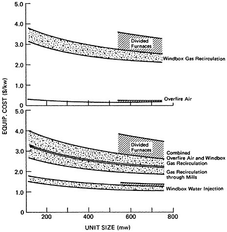
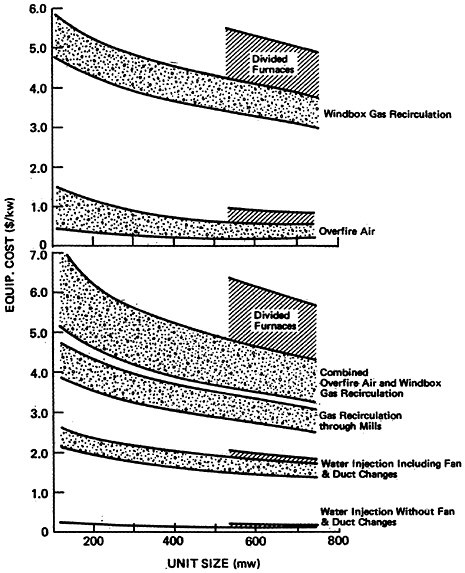
INDUSTRIAL BOILERS
Background
Boilers with capacities from 10 to 500 million BTU per hour emit an estimated 18.1 percent of the U.S. stationary source nitrogen oxides. The industrial boiler population is made up of about 75000 units of various types, ages, and applications which burn gas (57 percent of the energy supplied in 1968), coal, (23 percent) and oil (20 percent) (Lockling et al. 1974). Residual oils and a small quantity of distillate oils are used. As a result of regulations on the emissions of sulfur oxides, recent trends have been toward the use of natural gas and low sulfur oils in all but the largest units. However, due to increased prices and reduced availability of these fuels, the industrial sector may be forced to rely increasingly upon coal and residual oil.
About a third of the industrial boilers, accounting for 10 percent of the industrial capacity, are small units (10 to 16 million BTU per hour capacity) (Lockling et al. 1974). These are primarily packaged firetube boilers which burn oil or gas. The 17 to 100 million BTU per hour units, which are primarily packaged watertube boilers, account for 53 percent of the units and 45 percent of the capacity. The larger units are watertube boilers, mostly field erected. Currently only 1 percent of the units and 9 percent of the capacity are greater than 250 million BTU per hour capacity, the size range for which new source performance standards have been established.
The data on emission levels and combustion modification effectiveness for NOx control are limited, mostly derived from a field study performed by KVB, Engineering ((Cato et al.) in which about 80 units were tested for baseline emission levels and minimum NOx achievable without hardware modifications. Due to the limited flexibility in combustion operating conditions
for these units, only moderate reductions were obtained in most cases. The results are presented in Table 15–5.
When combustion modification strategies are considered, it will be necessary to consider several problems which may arise such as corrosion and deposits on boiler tubes, flame instability, blow-off, flashback, combustion driven oscillations, and combustion noise or roar. The need for tuning individual units to minimize these problems will place constraints on retrofit programs due to the large number of units in existence and their diverse characteristics (Lockling et al. 1974).
Gas-Fired Boiler Emissions
Gas-fired units without air preheat, firetube boilers, and some of the watertube boilers had NOx emission levels less than 0.14 lb NO2 /106 BTU. (Cato et al.) The watertube units with air preheat had generally higher emissions, from 0.08 to 0.45 lb NO2/106 BTU. By comparing units with different degrees of air preheat, it was estimated that the preheat effects vary from 0.02 lb NO2/106 BTU per 100F for units of less than 30 million BTU per hour capacity to 0.15 lb NO2/106 BTU per 100F for much larger units. (Cato et al.) This appeared to be a function of the burner firing rate (BTU/hr/ burner). Reducing the oxygen level had only a small effect on emissions from units without air preheat, but did decrease the NOx levels from preheated boilers. Off-stoichiometric firing, achieved by taking one burner out of service, resulted in NOx reductions of 16 to 42 percent. By combustion modification, the percentage of units with emissions below 0.2 lb NO2/106 BTU was increased from 75 percent to 82 percent, (Cato et al.)
Oil-Fired Burner Emissions
The baseline emission levels for those units fired with No. 2 fuel oil were 0.13 to 0.26 lb
TABLE 15–5
Uncontrolled NOx and Low NOx Emissions from Industrial Boilers (Cato et al.)
|
|
Baseline |
Low NOx |
|
||||||
|
Fuel |
Size MBH |
Burners |
Test Load MBH |
PPM @ 3% O2 |
|
PPM @ 3% O2 |
|
% reduction |
|
|
Type |
Number |
||||||||
|
Gas |
25 |
Ring |
1 |
20 |
72 |
.086 |
65 |
.077 |
10 |
|
Gas |
29 |
Ring |
1 |
22 |
70 |
.083 |
- |
- |
- |
|
Gas |
29 |
Ring |
1 |
11 |
97 |
.115 |
68 |
.081 |
29.6 |
|
Gas |
59 |
Ring |
6 |
48 |
116 |
.138 |
- |
- |
- |
|
Gas |
60 |
Ring |
2 |
48 |
101 |
.124 |
86 |
.102 |
17.7 |
|
Gas |
60 |
Ring |
4 |
46 |
242 |
.288 |
138 |
.164 |
43.1 |
|
Gas |
160 |
Ring |
1 |
136 |
374 |
.445 |
355 |
.423 |
4.9 |
|
Gas |
158 |
Ring |
4 |
125 |
299 |
.343 |
110 |
.131 |
61.8 |
|
Gas |
300 |
Ring |
4 |
259 |
199 |
.237 |
169 |
.201 |
15.2 |
|
Gas |
10 |
Ring |
1 |
8 |
55 |
.065 |
38 |
.045 |
30.8 |
|
Gas |
20 |
Ring |
1 |
14 |
107 |
.127 |
75 |
.089 |
29.9 |
|
Gas |
11 |
Ring |
1 |
10 |
87 |
.104 |
83 |
.099 |
4.8 |
|
Gas |
7 |
Ring |
1 |
6 |
71 |
.085 |
67 |
.080 |
5.8 |
|
Gas |
10 |
Ring |
1 |
7 |
91 |
.108 |
90 |
.107 |
.9 |
|
Gas |
13 |
Ring |
1 |
12 |
57 |
.068 |
- |
.067 |
1.5 |
|
Gas |
18 |
Ring |
1 |
17 |
56 |
.067 |
53 |
.063 |
6.0 |
|
Gas |
20 |
Ring |
1 |
13 |
79 |
.094 |
67 |
.080 |
14.9 |
|
Gas |
8 |
Ring |
1 |
6 |
70 |
.083 |
45 |
.054 |
35.0 |
|
Gas |
20 |
Ring |
1 |
10 |
101 |
.120 |
- |
- |
- |
|
Gas |
33 |
Ring |
1 |
24 |
90 |
.107 |
81 |
.096 |
10.3 |
|
Gas |
65 |
Ring |
6 |
53 |
98 |
.117 |
- |
- |
- |
|
Gas |
110 |
Ring |
1 |
85 |
94 |
.112 |
- |
- |
- |
|
Gas |
225 |
Nozzle |
8 |
180 |
212 |
.252 |
147 |
.175 |
30.6 |
|
Gas |
325 |
Nozzle |
8 |
260 |
320 |
.381 |
230 |
.274 |
28.1 |
|
|
Baseline |
Low NOx |
|
||||||
|
Fuel |
Size MBH |
Burners |
Test Load MBH |
PPM @ 3% O2 |
|
PPM @ 3% O2 |
|
% reduction |
|
|
Type |
Number |
||||||||
|
#2 Oil |
110 |
Steam |
2 |
88 |
177 |
.231 |
- |
- |
- |
|
#2 Oil |
10 |
Air |
1 |
7 |
169 |
.220 |
149 |
.194 |
11.8 |
|
#2 Oil |
18 |
Steam |
1 |
14 |
65 |
.085 |
63 |
.082 |
3.5 |
|
#2 Oil |
18 |
Air |
1 |
14 |
97 |
.127 |
86 |
.112 |
11.8 |
|
#2 Oil |
18 |
Mech |
1 |
12 |
80 |
.104 |
80 |
.104 |
- |
|
#2 Oil |
11 |
Air |
1 |
11 |
128 |
.167 |
- |
- |
- |
|
#2 Oil |
18 |
Air |
1 |
16 |
116 |
.151 |
- |
- |
- |
|
#2 Oil |
18 |
Steam |
1 |
16 |
118 |
.154 |
- |
- |
- |
|
#2 Oil |
20 |
Air |
1 |
16 |
193 |
.252 |
141 |
.184 |
27.0 |
|
#2 Oil |
29 |
Steam |
1 |
10 |
103 |
.134 |
- |
- |
- |
|
#2 Oil |
7 |
Air |
1 |
7 |
127 |
.166 |
- |
- |
- |
|
#2 Oil |
158 |
Steam |
4 |
115 |
181 |
.236 |
120 |
.157 |
33.5 |
|
#2 Oil |
33 |
Steam |
1 |
23 |
123 |
.160 |
104 |
.136 |
15.0 |
|
#2 Oil |
13 |
Air |
1 |
11 |
84 |
.110 |
- |
- |
- |
|
#5 Oil |
19 |
Cup |
1 |
12 |
200 |
.261 |
139 |
.181 |
30.7 |
|
#5 Oil |
85 |
Steam |
4 |
59 |
329 |
.429 |
243 |
.317 |
26.1 |
|
#5 Oil |
11 |
Air |
1 |
12 |
183 |
.239 |
162 |
.211 |
11.7 |
|
#5 Oil |
18 |
Air |
1 |
18 |
177 |
.231 |
154 |
.201 |
13.0 |
|
#5 Oil |
18 |
Steam |
1 |
17 |
161 |
.210 |
152 |
.198 |
5.7 |
|
#5 Oil |
13 |
Air |
1 |
11 |
181 |
.236 |
171 |
.223 |
5.5 |
|
#5 Oil |
7 |
Air |
1 |
7 |
275 |
.359 |
- |
- |
- |
|
#5 Oil |
59 |
Steam |
6 |
46 |
619 |
.807 |
516 |
.673 |
16.6 |
|
#5 Oil |
65 |
Steam |
6 |
50 |
466 |
.608 |
431 |
.562 |
7.6 |
|
#5 Oil |
125 |
Steam |
1 |
100 |
337 |
.440 |
322 |
.420 |
4.5 |
|
#5 Oil +RG |
110 |
Steam |
4 |
88 |
172 |
.224 |
166 |
.217 |
3.1 |
|
#5 Oil +RG |
110 |
Steam |
4 |
90 |
215 |
.280 |
211 |
.275 |
1.8 |
|
|
Baseline |
Low NOx |
|
||||||
|
Fuel |
Size MBH |
Burners |
Test Load MBH |
PPM @ 3% O2 |
|
PPM @ 3% O2 |
|
% reduction |
|
|
Type |
Number |
||||||||
|
NSF oil |
17 |
Cup |
1 |
15 |
184 |
.240 |
- |
- |
- |
|
#6 oil |
18 |
Steam |
1 |
14 |
350 |
.457 |
331 |
.432 |
5.5 |
|
#6 oil |
18 |
Air |
1 |
15 |
334 |
.436 |
277 |
.361 |
17.2 |
|
#6 oil |
80 |
Steam |
1 |
51 |
305 |
.398 |
268 |
.350 |
12.1 |
|
#6 oil |
90 |
Steam |
3 |
71 |
246 |
.321 |
175 |
.228 |
29.0 |
|
#6 oil |
65 |
Steam |
2 |
54 |
186 |
.243 |
174 |
.227 |
6.6 |
|
#6 oil |
105 |
Steam |
4 |
80 |
251 |
.327 |
222 |
.290 |
11.3 |
|
#6 oil |
260 |
Steam |
4 |
130 |
240 |
.313 |
201 |
.262 |
16.3 |
|
#6 oil |
500 |
Steam |
9 |
400 |
267 |
.348 |
180 |
.235 |
32.5 |
|
#6 oil |
7 |
Air |
1 |
7 |
298 |
.389 |
249 |
.325 |
16.5 |
|
O/C |
513 |
Cyc |
2 |
320 |
716 |
.934 |
- |
- |
- |
|
O/C |
513 |
Cyc |
2 |
320 |
710 |
.926 |
- |
- |
- |
|
Coal |
60 |
UFS |
7 |
48 |
266 |
.327 |
188 |
.263 |
29.3 |
|
Coal |
60 |
UFS |
7 |
46 |
224 |
.314 |
198 |
.277 |
11.8 |
|
Coal |
135 |
Sprd |
2 |
110 |
370 |
.518 |
335 |
.469 |
9.5 |
|
Coal |
50 |
Sprd |
1 |
40 |
465 |
.651 |
330 |
.462 |
29.0 |
|
Coal |
75 |
Sprd |
1 |
63 |
465 |
.651 |
387 |
.542 |
16.7 |
|
Coal |
225 |
Pulv. |
8 |
181 |
378 |
.529 |
360 |
.504 |
4.7 |
|
Coal |
210 |
Sprd |
5 |
120 |
553 |
.774 |
471 |
.659 |
14.9 |
|
Coal |
230 |
Sprd |
6 |
162 |
547 |
.766 |
360 |
.504 |
34.2 |
|
Coal |
500 |
Pulv |
6 |
400 |
580 |
.812 |
- |
- |
- |
|
Coal |
513 |
Cyc |
2 |
320 |
800 |
1.120 |
742 |
1.039 |
7.2 |
|
Coal |
10 |
UFS |
1 |
8 |
273 |
.382 |
- |
- |
- |
|
Coal |
10 |
UFS |
1 |
8 |
346 |
.484 |
- |
- |
- |
|
Coal |
325 |
Pulv |
8 |
260 |
484 |
.678 |
- |
- |
- |
|
Abbreviations NSF=Navy Standard Fuel Cup=Rotary cup fuel atomizer Air=Air assist fuel atomizer Steam=Steam-fuel atomizer Cyc=Cyclone furnace coal combustor UFS=Underfed stoker coal burning equipment Sprd=Spreader stoker coal burning equipment Pulv=Pulverized coal burning equipment MBH=Million BTU per hour |
NO2/106 BTU (Cato et al.). Increasing combustion intensity resulted in increased NOx, but other changes in operating parameters had little effect.
The heavy fuel oil emissions were higher, 0.20 to 0.81 lb NO2/106 BTU, and more sensitive to the operating conditions. The nitrogen content of the fuel had a particularly strong effect since an estimated 44 percent of the fuel nitrogen was converted to NOx. NOx emissions decreased with decreasing oxygen levels, burner heat release rate (BTU/hr/burner), and combustion intensity. Emission reductions of 6 to 29 percent were obtained by using stoichiometric or staged combustion. The technique of fuel atomization did not strongly influence the emissions as long as good atomization was achieved. The two highest emission levels for No. 5 oil were the result of preheating the oil to only 130F, rather than 160 to 180F as in most other tests. Increasing the oil temperature improved the atomizer effectiveness and reduced the NOx emission levels.
Coal-Fired Boiler Emissions
Due largely to the high nitrogen content of coals (1.29 to 1.80 percent by weight in the KVB study), the emissions from coal-fired units were generally higher than those from oil or gas fired units, i.e., 0.31 to 1.12 lb NO2/106 BTU. (Cato et al.) The lowest emissions from coal-fired units were from underfed stoker coal burning equipment. In these units the air fed up through the grating is insufficient for complete combustion, so additional air must be introduced above the grating through overfire air ports. The combustion is, therefore, effectively staged, and the NOx emissions were quite low, .31 to .48 lb NO2/106 BTU.
Spreader stokers, in which the fuel is introduced with the air flow above the grate, had intermediate emission characteristics, 0.52 to 0.77 lb NO2/106 BTU. Some of the fuel is burned in the fuel spray; the remaining fuel is burned on the grate as in the underfed stoker. The
resultant combustion is only partially staged. The combustion intensities are also higher than for underfed stokers, possibly increasing thermal NO formation.
Pulverized coal units, in which all of the fuel is burned in suspension, had higher emissions, 0.53 to 0.81 lb NO2/106 BTU. A unit equipped with two cyclone-type coal combustors produced 1.12 lb NO2/106 BTU, the highest emissions of all the units tested due to the very high combustion intensity. (Cato et al.)
Reductions of about 0.07 lb NO2/106 BTU percent reduction in oxygen were obtained by reducing the amount of excess air. A decrease in underfire air-rate with a compensating introduction of air through openings higher in the furnace for a spreader stoker-fired boiler resulted in about a 46 percent NOx reduction, but the grate temperature increased beyond its allowable limits. The most acceptable operating conditions reduced NOx by 20 to 25 percent. Controlled NOx emissions were below 0.68 lb NO2/106 BTU for all but the cyclone fired boiler. (Cato et al.)
RESIDENTIAL AND COMMERCIAL SPACE HEATING
Background
Space heating equipment of less than 10 million BTU hr capacity emits about 7.1 percent of the U.S. stationary source NOx. The emissions are largely near ground level in areas of high population densities. (Hall et al. 1974). The problem of NOx emission from these sources may, in fact, be more severe than this number would indicate since the emissions are confined to the heating season.
Commercial units, which generally fall in the range of 0.3 to 10 million BTU hr capacity, include a mix of packaged firetube, cast iron, and watertube boilers. (Barrett et al. 1973). These units are equipped to burn natural gas (56 percent), number 2 oil (38 percent), number 4 and 5 oils (8 percent), and number 6 oil (4 percent). About 6 percent of the units have dual
fuel capabilities. Commercial boilers are designed to operate with a minimum of manual control and maintenance for a life of from 10 to 45 years depending upon the type of unit.
Residential units are much smaller; about 70 percent have capacities of less than 0.2 million BTU/hr, and 96 percent have capacities of less than 0.42 million BTU/hr. (Barrett et al. 1973). The units include warm air furnaces hot-water and steam boilers, and water heaters, and are fueled primarily by distillate oil (No. 2) or natural gas. Operation is generally controlled by a thermostat and maintenance is on an annual schedule, at most.
Emissions from Residential Space Heating Equipment
Specific NOx emission levels from residential units average about 0.14 lb NO2/106 BTU, (Barrett et al. 1973) which is low, primarily as a consequence of low combustion intensities in these units. About 90 percent of the residential units tested in a recent field survey (Barrett et al. 1973) of oil-fired space heating equipment had emissions below 0.2 lb NO2/ 106 BTU; the highest emission level measured in that survey was about 0.29 lb NO2/106 BTU. Normal service and adjustment practice had very little effect on the emission level of NOx or any pollutant other than smoke.
A recent EPA study (Hall et al. 1974) (USEPA 19) provides more detailed information on the effects of operating conditions and burner design on residential heating equipment emissions. Combustion improving devices, which utilize flame retention to produce a more intense flame region, tend to increase efficiency and to increase NOx emissions. A spark ignition system was found to produce between 7 and 10 percent of the NOx due to continuous operation of the ignition arc during the burning cycle. Turning the ignition system off after startup, or using low power output ignition could eliminate this source. Other modifications to existing equipment designs were found
to have very little effect in this study. However, significantly lower levels of NOx emissions have been demonstrated without increases in other pollutant emissions, or loss of efficiency with both optimized operation of conventional systems (Dickerson and Okuda 1973), and new combustor concepts (Dickerson and Okuda 1974, Hall et al. 1974, Thompson et al. 1973). In a recent EPA-sponsored program, Rocketdyne has developed low emission burners based on conventional design practices. (Dickerson and Okuda 1974). One unit tested for 128 hours was a 20000 BTU/hr, residential size burner which produced about 0.048 lb NO2/106 BTU. A commercial size, 180,000 BTU/hr, unit was also tested for 112 hours and produced only 0.025 lb NO2/106 BTU. Burners which use hot combustion products to prevaporize the liquid fuel can achieve very low levels of all pollutants with 0.02 to 0.07 lb NO2/106 BTU during steady state operation. During startup, however, the fuel vaporization is not effective in some systems and the CO and smoke emissions are high. Internal recirculation of combustion products is also very effective in reducing thermal NOx formation by reducing flame temperatures. NOx emissions as low as 0.015 lb NO2/ 106 BTU have been reported. The lowest emission levels reported, less than .005 lb NO2/106 BTU, have been achieved using catalytic combustion; (Dickerson and Okuda 1974, Thompson et al. 1973), however, the associated hydrocarbon emissions were very high. These studies have demonstrated that very low NOx emission levels are achievable for residential and commercial heating units. However, further development will be required before these systems become practical for wide scale application.
Emissions from Commercial Boilers
The specific NOx emissions from commercial boilers fired with natural gas or No. 2 oil are comparable with the emissions from residential units, i.e., 0.07 to 0.20 lb NO2/106 BTU,
(Barrett et al. 1973). Combustion of residual oils, No. 4, 5, or 6 oil, resulted in emissions as high as 0.47 lb NO2/106 BTU in a Battelle field study, (Barrett et al. 1973) primarily due to the nitrogen content of these fuels, about 60 percent of which was converted to NOx.
For heavy oil combustion, reduced excess air resulted in reduced NOx emissions, but also high smoke and carbon monoxide emission levels. Techniques such as staged and low excess air combustion which have been applied for fuel NOx control in utility boilers might be adaptable to large commercial boilers, but have not been applied to date. Switching to low nitrogen content fuels, such as natural gas and No. 2 oil, if they are available, would be one means of NOx control for commercial units for which modification of the combustion process is not feasible. New combustion concepts such as prevaporization of the fuel or surface combustion also have potential for commercial units, but have not been demonstrated.
INTERNAL COMBUSTION ENGINES
Types and Locations
Internal combustion engines produce about 21.3 percent of the total stationary source NOx emissions, second only to utility boilers (Martin 1974). The installed capacity of stationary engines is distributed about equally between reciprocating engines (34.7 million horsepower) and gas turbines (35.5 million horsepower) (McGowin 1973). The applications and NOx emissions of these two classes of engines are quite different. Estimates of power generation by engines indicate that reciprocating engines, generate about 71.8 percent of the power while gas turbines generate the remaining power (McGowin 1973) corresponding to utilization of 58 and 22 percent, respectively, of their installed capacities. Emission estimates for these two sources are somewhat uncertain, particularly for gas turbines whose total emissions have been estimated at 131 (Martin 1974)
to 291 (McGowin 1973) thousand tons of NOx per year. Nonetheless, it is clear that reciprocating engines produce the vast majority of the stationary engine emissions.
Recent survey estimates (McGowin 1973) of the installed power, fuel usage, emissions, and power generation for stationary engine applications are tabulated in Table 15–6. In terms of installed horsepower, the major uses of engines are electric power generation (54.8 percent), oil and gas pipelines (22.4 percent), agriculture (10.7 percent), natural gas processing (5.6 percent) and production (4.6 percent). The major sources of stationary-engine NOx emissions are oil and gas pipelines (41.6 percent), natural gas processing (19.2 percent), and natural gas production (13.8 percent) which use primarily spark ignition gas engines, and agriculture (14.2 percent) which uses primarily diesel engines. Electric power generation, which accounts for most of the installed horsepower, produces only about 5 to 10 percent of the stationary engine NOx due to two factors:
-
the overall load factor for engines used in electric power production is only 12 percent since the primary application of such engines is for peak and stand-by power generation; and
-
most of the installed horsepower is in the form of gas turbines which produce much lower NOx emissions than reciprocating engines. Reciprocating engines are used for peak power generation in older installations and continue to find application for electricity generation in municipalities, hospitals, schools and shopping centers which are too small to use gas turbine units. In recent years, both large electric utilities and natural, gas pipelines have been favoring large gas turbines.
Recent projections from the electric utility industry (NERC 1974) for the period 1974–1983 indicate a 75 percent increase in the gas turbine generating capacity and a four-fold increase in electric power generated by gas turbines for continuous power generation in addition to peak power generation. This will be accompanied by slightly reduced usage of natural gas and increased usage of both
TABLE 15–6
Stationary Engines in the United States (McGowin 1973)
|
|
Installed Horsepower—103 Bhp |
Fuel Consumptiona 1012 Btu |
||||||
|
|
Load Factor % |
Diesel |
Fuel |
Gas Engine |
Gas Turbine |
Total |
Natural Gas |
No. 2 Oil |
|
Electric Power |
12 |
1,570 |
3,710 |
90 |
30,440 |
35,810 |
127.24 |
280.14 |
|
Oil & Gas Pipeline |
69 |
830 |
390 |
10,990 |
3,520 |
15,730 |
802.06 |
40.77 |
|
Natural Gas Processing |
- |
- |
- |
2,410 |
1,530 |
3,940 |
432.60 |
- |
|
Oil & Gas Exploration |
15 |
1,500 |
- |
500 |
- |
2,000 |
5.09 |
14.67 |
|
Crude Oil Production |
- |
- |
- |
852 |
- |
852 |
42.66 |
- |
|
Natural Gas Production |
- |
- |
- |
3,237 |
- |
3,237 |
190.04 |
- |
|
Agricultural |
40 |
7,500 |
- |
- |
- |
7,500 |
- |
198.94 |
|
Industrial Process |
- |
- |
- |
230 |
- |
230 |
11.88 |
- |
|
Municipal Water & Sewage |
75 |
465 |
- |
465 |
- |
930 |
24.08 |
23.14 |
|
TOTAL |
|
11,865 |
4,100 |
18,774 |
35,490 |
70,229 |
1635.75 |
557.66 |
|
(a)Calculated ing Higher ating es of 5.8×10⁶ Btu/Bbl for oil and 1070 Btu for natural gas. |
||||||||
|
Power Generation 106 Bhp hr |
Annual NOx Emissions Tons |
Emission Factors gm NOx/bhp hr |
||||
|
Recip |
Gas Turbine |
Recip |
Gas Turbine |
Total |
Recip |
Gas Turbine |
|
5,900 |
33,240 |
62,440 |
62,920 |
125,360 |
9.61 |
1.72 |
|
73,700 |
21,260 |
39,800 |
39,800 |
970,000 |
11.46 |
1.70 |
|
31,280 |
15,010 |
429,690 |
28,130 |
457,820 |
12.47 |
1.70 |
|
2,580 |
- |
31,720 |
- |
31,720 |
11.16 |
- |
|
5,410 |
- |
62,370 |
- |
62,370 |
10.47 |
- |
|
24,100 |
- |
308,200 |
- |
308,200 |
11.61 |
- |
|
26,280 |
- |
318,700 |
- |
318,700 |
11.01 |
- |
|
1,510 |
- |
19,300 |
- |
19,300 |
11.61 |
- |
|
6,110 |
- |
76,100 |
- |
76,100 |
11.31 |
- |
|
176,870 |
69,510 |
2,238,720 |
130,850 |
2,369,570 |
- |
- |
|
|
Per cent |
Capacity |
|
|||
|
58.12% |
22.36 |
|||||
distillate and residual oils as gas turbine fuels. (NERC 1974).
Large concentrations of stationary engine horsepower, e.g., 10,000 to 60,000 Bhp, reciprocating engines at some pipeline compressor stations, may represent significant local pollution sources. Most pipeline compressor stations are remote from population centers; however, there is some human exposure at most compressor stations and the NOx levels may be high (McGowin 1973).
Stationary reciprocating engines can be classified in several categories. The fuel/ air mixture may be ignited in reciprocating engines by either an electrical spark discharge (spark ignition engines) or by compression heating (diesel engines). Natural gas engines are almost always spark ignited. In diesel engines combustion is controlled by injecting fuel into the cylinder through a spray nozzle at the proper time during the compression stroke. Dual fuel engines can operate on 100 percent fuel oil or natural gas to which fuel oil has been added (about 5 percent on the basis of heating value) to serve as a pilot for ignition.
Stationary gas turbines have evolved from aircraft jet engines. In its simplest form, the gas turbine engine (simple cycle) consists of a compressor in which the air is compressed from 100 to 200 psig, followed by a combustor in which fuel (liquid or gaseous) is added. Combustion occurs at mixtures of fuel and air which are overall very fuel lean. The combustion gases are then expanded through a turbine or turbines to near atmospheric pressure, converting their energy to power. The simple cycle gas turbine thermal efficiency is 24 to 31 percent. The efficiency of the gas turbine can be increased by further extraction of heat from the exhaust gases which normally leave the turbine at 800 F to 1100F. In a regenerative cycle this is done by passing the air leaving the compressor through a heat exchanger in which some of the heat of the exhaust gases leaving the turbine is transferred to the pressurized air. In such a cycle less
fuel is required for fixed turbine inlet temperatures increasing the thermal efficiency to about 34 to 38 percent. Another way of utilizing the exhaust waste heat is in a combined cycle. In this case the exhaust gases are used to produce steam which can then be used to drive a steam turbine to produce additional power. Due to its high thermal efficiency, currently 40 to 42 percent, the combined cycle gas turbine is being favored by electric utilities in new installations.
Emission Levels
Table 15–7 summarizes the emission factors used in the estimates of exhaust emissions from stationary engines described above. While there is considerable variation in the emissions, indicated by the numbers in parentheses, these figures provide a useful basis for comparison of the uncontrolled emission levels of the various engines.
Except for gas turbines and prechamber diesel engines, the NOx levels, in the range 2.8–4.2 lb NOx/106 BTU, exhibit only minor differences among the different engine types (McGowin 1973). Turbocharging results in slight increases in NOx emissions over naturally aspirated engines due to increased temperatures. Prechamber diesel engines, in which combustion is initiated in a fuel rich environment, emit about half as much NOx as direct injection diesels.
Gas turbine NOx emissions are one-tenth the emissions of reciprocating engines, primarily as a result of lower peak temperatures and shorter residence times in the combustion chamber. Emissions from distillate-oil fired gas turbines are about a factor of two higher than emissions from gas turbines fueled with natural gas (Johnson and Schiefer, Roessler et al. 1974). Since the electric utility projections indicate increasing reliance on oil as gas turbine fuel, including residual oils as a substantial fraction of total fuel by the mid-1980’s (NERC 1974), the uncontrolled specific
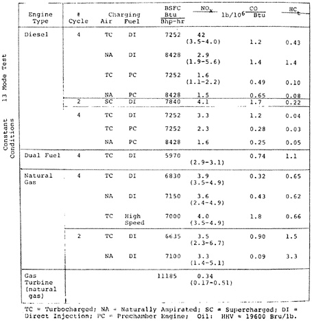
emissions for gas turbines may be expected to increase. Fuel-nitrogen may play an important role in determining the achievable emission levels, since the limited data available on fuel-NOx formation in gas turbines suggests a high conversion efficiency of fuel-N to NOx (Fenimore 1972, Dilmore and Rohrer 1974).
NOx Emission Control Technology
Many emission control techniques which have been developed for mobile sources are potentially applicable to stationary engines; however, different design constraints may make techniques either more or less desirable for stationary engines than for mobile engines. Size and weight constraints are severe for mobile engines, and durability is an important characteristic of an engine used in stationary applications. Techniques to reduce NOx include engine derating, fuel injection and ignition timing retard, exhaust gas recirculation, catalytic converters, water or steam injection, and engine component and operating condition modifications. Methods developed or evaluated for mobile-source NOx-control may be applicable to stationary engines, but the emission control achievable and the operating parameters in stationary applications cannot be directly inferred from data obtained on smaller mobile engines. Since the carbon monoxide and unburned hydrocarbon emissions of large, stationary, reciprocating engines tend to be quite low, moderate increases in these emissions due to NOx control may be acceptable although this must be determined on a case-by-case basis.
A detailed discussion of control techniques for various engine types appears in Appendix 15-A but the major conclusions are summarized here. In diesel engines, adjustment of the fuel injection timing can reduce NOx emissions by about 40 percent without major hardware alteration. The NOx reduction is accompanied by increases in fuel consumption and in carbon monoxide emissions. Cooling the intake air can reduce NOx emissions and improve
fuel economy. Optimization of the fuel injection system may produce modest reductions (20 percent for one engine) in NOx without increasing fuel consumption.
Diesel NOx emissions can also be reduced by as much as 50 percent by water injection into the intake system with very little change in fuel consumption but corrosion problems must be resolved before water injection techniques become useful for stationary engines.
Exhaust gas recirculation (EGR) has been shown to be a very effective NOx abatement technique for diesel engines. Fifty percent reductions in NOx emissions have been achieved using EGR with only a small penalty in fuel consumption. However, the NOx emission reductions are accompanied by a 100 to 150 percent increase in carbon monoxide and smoke.
NOx can be removed from diesel exhaust gases by catalytic reduction. Very high removal efficiencies have been observed but the costs are high and significant development work will be required before wide scale application will be practical.
In spark ignition engines, a fuel rich mixture results in low NOx emissions at the expense of increased carbon monoxide and hydrocarbon emissions and of increased fuel consumption. Stratified charge engines offer the possibility of substantially reduced emissions as well as reduced fuel consumption.
Reducing the temperature of the fuel/air mixture in a spark ignition engine results in a moderate reduction in NOx emissions while reducing fuel consumption. Water injection can reduce the NOx emissions by as much as 80 percent, but this may be accompanied by a significant increase in fuel consumption. Exhaust gas recirculation can reduce NOx emissions by as much as 80 percent, but the fuel economy loss is considerable. Recirculating only five to ten percent of the exhaust gas and advancing the spark timing can minimize the loss, making 40 percent reductions in NOx emissions possible.
For all techniques designed to reduce NOx emissions from spark ignition engines, the effects on engine durability must be determined
before long term use on stationary engines is practical. A meaningful assessment of the cost of emission control for large stationary gas engines has not yet been performed.
Water or steam injection has been shown to be a very effective technique for stationary gas turbine NOx emissions. For small gas turbines (less than 2 Mw) the costs of this technique may be prohibitive. NOx reductions of 50 to 75 percent have been achieved with water injection with only slight increases in carbon monoxide emissions. Water injection is currantly being used by some utilities without observed deleterious effects as long as the water purity is maintained at a high level.
INDUSTRIAL PROCESSES
Industrial Process Heating
It is estimated that industrial process heating contributed 3.3 percent of total stationary source emissions in 1972. The sources include open-hearth furnaces with high air-preheat used for glass-melting and to a decreasing extent in steel making; rotary, vertical, and tunnel kilns used in cement, lime, and ceramic industries; pyrolysis process furnaces for ethylene and propylene production; petroleum heaters, cat-cracking regenerations, and CO boilers in the petroleum industry; billet-reheating and ingot-soaking furnaces, coke-ovens and blast furnaces in the steel industry; and a large variety of heat-treatment furnaces in the metallurgical industry. The emissions from these sources have not been well documented. In view of the small contribution to the total national emissions of NOx and the diversity of sources, the control of emissions from process heating furnaces has received comparatively little attention other than through the development of low-emission burners by the equipment manufacturers that supply the combustion equipment. The applicability of combustion modification techniques to process-heaters depends upon the specific heater design and no
generalizations can be made at present about the potential for control of emissions from these sources.
Non-Combustion Sources
The major non-combustion sources of NOx are the manufacture and use of nitric acid which were estimated to contribute 1.3 percent of the stationary source emissions in 1972. The techniques for controlling NOx emission from non combustion-sources are based on removal of the NOx from the tail gas by selective or non-selective reduction, adsorption, and absorption. Uncontrolled emissions from nitric acid plants are in the range of 2000 to 3000 ppm (approximately 28 to 41 lbs per ton of acid) and are characterized by approximately equal concentrations of NO and NO2. As a consequence of the cost of installation of tail-gas treatment processes to meet emission standards of 3.0 lbs/ton of acid for new plants, nitric acid plants are being designed to yield lower concentration effluents.
The most commonly used emission-control technique at present is the catalytic combustion of the NOx using a fuel, generally natural gas, and a platinum or palladium catalyst (Bartok et al. 1969, Gillespie et al. 1971). In this process sufficient fuel must be supplied to consume the oxygen present in the tail-gas and part of the energy released is recovered in a waste heat boiler and/or a power recovery turbine. A selective reduction technique has been developed using ammonia to reduce the NOx without consuming the oxygen. For this technique to work, the catalyst bed temperature must be carefully controlled and maintained in the range of 410F to 520F. Several selective abatement techniques have been installed on commercial units (Bartok et al. 1969).
A commercial adsorption process has been developed utilizing a molecular sieve bed to catalytically convert NO to NO2 and to adsorb the NO2 product. Continuous operation is
achieved through the use of two beds in an adsorption-desorption cycle. The NO2 is recycled to the nitric acid plant. High recovery efficiencies are claimed for this process at costs competitive with catalytic reduction (Fornoff 1972). Two units have been installed on commercial plants.
Absorption techniques for NOx are hindered by the relatively low solubility of NO. A process enhancing the absorption of NOx by catalyzing the oxidation of NO to NO2 has been commercialized (Mayland and Heinze 1973).
For typical NOx concentrations in a tail gas of about 3000 ppm, the methods described above can achieve over 90 percent removal. The best abatement technique for a given unit depends on the specific conditions at a plant. Investment and operating costs are of the order of $1500/ton-per-day capacity and $1.50 per ton of acid produced, but vary greatly with location, size, and design of a unit.
FLUIDIZED BED COMBUSTORS
State of Development
The combustion of coal in fluidized beds operated in the temperature range of 1400F to 2000F appears to have a number of advantages over conventional utility pulverized-coal boilers with stack-gas clean-up. These advantages include:
-
high heat release rates per unit volume permitting the construction of relatively compact boilers without penalizing the over-all combustion efficiency;
-
high rates of heat transfer to tubes immersed in the bed and, therefore, a relatively small tube surface area;
-
sulfur dioxide removal capabilities of 80 to 95 percent by injection of limestone or dolomite in the bed;
-
operation below the ash softening temperatures and, hence, elimination of slagging problems and a reduction in emissions of hazard-
-
ous trace metals [operation at temperatures above 2050F may be used, however, to promote self-agglomeration of the ash (Ehrlick et al. 1974)];
-
use of coarsely pulverized coal in contrast to under 200 mesh for a pulverized-coal boiler;
-
low nitrogen oxide emissions;
-
potential for increased cycle efficiency by use of pressurized boilers in a combined steam/gas-turbine cycle; and
-
ability to handle low-grade solid fuels
Studies of fluidized bed combustion for coal burning were initiated in 1961 by the National Coal Board in England on small-scale units operated at pressures from atmospheric up to 6 atmospheres (Hoy and Roberts 1969, Broadbent 1970). In 1965, work was initiated in the U.S. at Pope, Evans, and Robbins under contract to the Office of Coal Research (Bishop et al. 1966). With the recognition of the potential of fluidized bed combustion for reducing the emissions of sulfur and nitrogen oxides, the U.S. program has expanded to include a number of organizations working under the sponsorship of the Office of Coal Research and the Environmental Protection Agency.
A number of system design studies for the use of pulverized combustion have been conducted by Pope, Evans, and Robbins (Bishop et al. 1966, Bishop et al. 1968, Bishop et al. 1972, Ehrlich et al. 1974, Ehrlich and Chronowski 1974, Ehrlich and McCurdy, Ehrlich et al. 1971, Ehrlich 1970), Westinghouse (Archer et al. 1971), and Foster-Wheeler (Gamble 1974). These studies lead to the conclusion that fluidized bed combustion offers its greatest potential in competition with conventional fossil-fuel utility boilers using low-sulfur fuel or stack-gas clean-up. The economic analyses indicate that the pressurized units used in combined cycles have greater potential in the long-range than the atmospheric pressure units. The development of atmospheric pressure combustors is, however, more advanced and a 30 MW unit is scheduled for completion in 1975 in Rivesville, Virginia. Depending on the successful operation of this
cell, it is expected that multicellular 200 MWe units will be installed before 1980 and 800 MWe units shortly thereafter. It is anticipated that the installation of pressurized units will follow the atmospheric-pressure units. It is clear that the acceptance by the utility industries of the fluidized bed combustors will depend greatly on whether or not these units will be able to match the relatively trouble-free operation of conventional pulverized-coal units.
NOx Emissions from Fluidized-Bed Combustors
Fluidized-bed combustors have the potential of meeting the existing standards for NOx emissions from coal-fired steam-generating plants by a considerable margin. However, the factors that control these emissions are imperfectly understood. At the temperatures of the fluidized bed negligible amounts of thermal NOx are expected and the major source of NOx emission is the fuel nitrogen. This has been proven conclusively in tests at the Argonne National Laboratories which showed no change in NOx concentrations from a fluidized-bed coal combustor when the nitrogen in the combustion air was replaced by argon (Jonke et al. 1969). The emissions from fluidized bed combustors are therefore a function of both the fuel nitrogen content and the fraction of fuel nitrogen converted to NOx during combustion. Many factors influence the conversion of fuel nitrogen to NOx. Tests on a batch laboratory reactor have shown that part of the NOx is contributed by oxidation of the volatiles emitted by the coal and the remainder by oxidation of the char, with the fractional contribution of the volatiles increasing with increasing temperature (Pereira et al. 1974). The emissions from laboratory and pilot units have been found to increase with increasing temperature and increasing excess air (Hammons and Skopp 1971, Jonke et al. 1969, Jonke et al. 1970, Jonke et al. 1971). Increased pressure in some cases yields lower emissions (Vogel et al. 1974). The emissions of NOx from the beds are also found to be a function of the composition of the solids in the bed. Calcium sulfate
catalyzes the reduction of nitrogen oxide with carbon monoxide and the emissions from a bed using calcium sulfate as a bed material are lower than the corresponding emissions with an alundum bed material (Hammons and Skopp 1971). In addition a partially sulfated lime is found to reduce nitric oxide (Hammons and Skopp 1971). Some additives, such as cobaltic oxide, however, cause the emissions to increase (Jonke et al. 1970, Jarry et al. 1970), possibly as a consequence of catalysis of the oxidation of the fuel nitrogen. Representative values of emissions for a range of conditions are shown in Table 15–8.
Emission levels of 0.10 to 0.17 lbs NO2/106 BTU have been attained in both atmospheric and pressurized combustors operated slightly fuel lean (15 percent excess air or 3 percent oxygen) (Demski et al. 1973, Vogel et al. 1974). Other atmospheric pressure tests have yielded higher emissions than these although the emissions were still lower than the standard for coal units (Hammons and Skopp 1971). If needed, significant additional reduction in NOx emissions may be attained in fluidized bed combustors by the use of staged combustion (Hammons and Skopp 1971)
TALL STACKS AND INTERMITTENT CONTROLS FOR NITROGEN OXIDES
Until recently the U.S. Environmental Protection Agency has consistently argued against intermittent controls as a means of achieving compliance with air quality standards. As several states have reviewed the cost-effectiveness of their clean fuel regulations, intermittent controls have gained more support. The use of tall stacks and of intermittent controls (such as fuel switching and load switching) has been directed primarily toward the control of sulfur dioxide emissions and their effects and, to a lesser extent, toward particulate emission control. This section reviews the applicability of tall stacks and intermittent controls to achieve compliance with NOx standards or to reduce photochemical smog formation.
TABLE 15–8
NOx Emissions from Fluidized Bed Combustors (Jonke et al. 1974, Skopp et al. 1971)
|
T(OF) |
O2 (%) |
Pressure (atm) |
|
% N in FUel |
Comments |
|
1500 |
6–7 |
1 |
0.11 |
|
|
|
1500 |
4 |
1 |
0.11–0.17 |
||
|
1400 |
4 |
1 |
0.45 |
1.4 |
CaSO4 bed material |
|
1500 |
4 |
1 |
0.80 |
1.4 |
" " " |
|
1800 |
4 |
1 |
0.99 |
1.4 |
" " " |
|
1600 |
1 |
1 |
0.81 |
1.4 |
" " " |
|
1600 |
4 |
1 |
0.95 |
1.4 |
" " " |
|
1600 |
6 |
1 |
1.05 |
1.4 |
" " " |
|
1600 |
8 |
1 |
1.12 |
1.4 |
" " " |
|
1600 |
1 |
1 |
1.05 |
1.4 |
Alundum bed material |
|
1600 |
4 |
1 |
1.12 |
1.4 |
" " " |
|
1600 |
6 |
1 |
1.19 |
1.4 |
" " " |
|
1600 |
8 |
1 |
1.26 |
1.4 |
" " " |
|
1445 |
2.7 |
8 |
0.27 |
1.1 |
|
|
1565 |
3.0 |
8 |
0.29 |
1.1 |
|
|
1575 |
3.0 |
8 |
0.20 |
1.1 |
|
|
1650 |
3.0 |
8 |
0.25 |
1.1 |
|
|
1460 |
3.0 |
8 |
0.21 |
1.1 |
|
|
1565 |
3.0 |
8 |
0.27 |
1.1 |
|
|
1550 |
3.0 |
8 |
0.22 |
1.1 |
|
|
1460 |
2.7 |
8 |
0.21 |
1.1 |
|
|
1630 |
3.0 |
8 |
0.38 |
1.1 |
|
|
1665 |
2.9 |
8 |
0.17 |
1.1 |
Tall Stacks: The Effects of Elevated Release on Nitrogen Oxides
Tall stacks (greater than 500 feet) have been proposed as possible control methods for sulfur dioxide but their use may have an effect on nitrogen oxides. For pollutants with long half-lives (several hours to several days) predicted ground level concentrations of pollutants are reduced significantly by the use of taller stacks. As seen in Figure 15–6, increasing the effective stack height by a factor of 10 decreases the predicted maximum downwind concentration by two orders of magnitude. Of course, there are many simplifying assumptions in these calculations, for example the existence of flat terrain, which restrict their direct application.
Moreover, air pollutants are not chemically inert. Nitric oxide is oxidized to nitrogen dioxide which can dissolve in water droplets to form nitric acid. The acid is neutralized to nitrates, and the nitrates are eventually deposited on the surface. The conversion times for nitric acid and nitrate formation are a factor of three to four times faster than those for sulfuric acid and sulfates, the result of similar processes which occur with sulfur dioxide emissions. Thus secondary nitrogen oxide products such as nitric acid can potentially have a much more serious impact in the vicinity of the source than sulfur oxide decay products.
The effects of tall stacks on the formation of secondary pollutants is somewhat speculative. Assume that these stacks will service large, high efficiency combustion processes, for example power plants. Hydrocarbon and carbon monoxide emissions should therefore be extremely small. The NO emissions at higher levels will be separated from the ground level hydrocarbon and carbon monoxide automobile emissions. Hydrocarbons and carbon monoxide are important in the production and recycling of the transient radicals which drive the net dynamic balance equation to the conversion of NO to NO2 as shown in Chapter 14, Appendix 14-A. Calvert (1973), for example, has shown in numerical simulations, that if hydrocarbons are absent, decreased CO concentra-
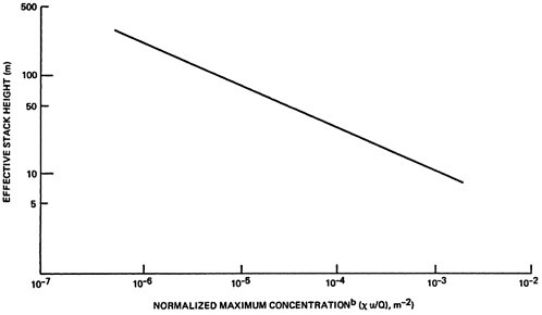
tions lower the maximum levels of NO2 and O3.
On the other hand, tall stacks may release NO into regions rich in ozone. Coffey and Stasiuk (1975) have recently suggested that urban peak ozone concentrations are primarily a result of high background levels of ozone rather than local photochemical production. They argue that since urban areas are major sources of nitric oxide, they act as sinks for ozone. Maximum surface ozone levels are associated with maximum downward mixing. Unpublished night ozone measurements by the authors show uniform ozone levels from just above the ground to 5,000 feet and peak values occurring in a haze layer between 5,000 and 5,500 feet. (See Figure 15–7.)
Davis et al. (1974) have tracked a power plant plume from two 200 meter stacks. Ambient ozone concentrations at this level had been consistently 60 to 80 ppb for several days. These high ozone levels produced rapid NO to NO2 conversion. Ozone was completely depleted in the plume out to 24 km downwind. However beyond this point ozone concentrations in the plume began to rise, eventually exceeding ambient levels out of the plume by 20 ppb. In the absence of hydrocarbons and carbon monoxide, the authors have suggested a photochemical reaction scheme with the sulfur oxide emissions to account for the long distance O3 generation. Altshuller (1974) has suggested that the entrainment of ambient air containing hydrocarbons and carbon monoxide allows the classical photochemical reactions to occur after sufficient dillution of the plume.
At present, there are not enough field measurements to determine the relative effects of near ground level and high level nitrogen oxide emissions. There is evidence that high level sources (power plant plumes) may lead to increased ozone many kilometers downwind but field studies are needed to assess rural and urban oxidant levels as well as their vertical distribution.

Intermittent Control Strategies
The use of intermittent methods and procedures for NOx controls is limited for the following reasons:
-
although fuel switching is successfully being employed to control ambient sulfur dioxide levels, the organic nitrogen component of fossil fuels varies only from 0.1 percent for distillate oils to greater than 2 percent for Colorado shale residual oil and bituminous coal: this range is far smaller than the natural variation in the amount of sulfur in fossil fuels;
-
there are at present no processes available which can readily and economically remove nitrogen from the fuel;
-
unlike sulfur dioxide, which is formed entirely from oxidation of sulfur in the fuel, some nitrogen oxides originate from thermal fixation of air N2 during high temperature combustion so that nitrogen oxides can be emitted even in the absence of fuel nitrogen;
-
while fuel switching based on meteorological parameters to meet one-hour, three-hour and 24 hour sulfur dioxide standards (depending on the state) can be economical for large fuel consumers with dual fuel storage capacity, there are no short term Federal ambient air quality standards for NOx. The need for fuel switching would have to be determined on the basis of predicted or measured photochemical oxidant levels. Episodes of high oxidant concentrations can last several days, but the annual frequency of such occurrences is quite low (less than 0.01) for most of the country. It is unlikely that large storage capacity could be devoted to low nitrogen-content fuels when the use of such fuels would be rare;
-
because of complicated reactions between NOx and other pollutants, the prediction of ground level NOx or
-
photochemical oxidant concentrations is very uncertain.
In spite of these limitations, there are some situations in which NOx may be dynamically controlled. Further, through allocation of low nitrogen content fuels some reduction of NOx emissions may be realized. Intermittent or supplementary control techniques applicable to NOx emission reductions are summarized in this section.
Fuel Type Substitution: Oil for Coal
The nitrogen content of distillate oil averages 0.1 percent, residual oil 0.4 percent and coal 1.4 percent. On this basis it would appear that fuel conversion may lower NOx emissions (Archer et al. 1971, Armento and Sage 1973a, Armento and Sage 1973b, Armento 1974, Axworthy and Shuman 1973, Bagwell et al. 1970, Barnhart and Diehl 1959). However, this is not necessarily the case. On a BTU rating, the emissions from existing coal and residual oil fired units of comparable size are sometimes nearly equivalent. (See Table 15–9, which summarizes EPA emission factors based on contractors’ fuel tests.) There is an emission factor difference between new utility coal and oil fired units; in new plants, for coals NOx emission limitations are 0.7 lbs. per million BTU’s, and for oil the NOx emission limitations are 0.3 lbs. per million BTU’s.
However, this 0.4 lbs. per million BTU advantage (57 percent) would be difficult to achieve simply by changing fuels. The lower emissions factor for new utility boilers is a result of new design characteristics. This design advantage may be inappropriate for maintaining lower emission rates if fuel is switched.
Fuel Type Substitution: Gas for Oil, Gas for Coal
The new source NOx emission limitation for
TABLE 15–9
NOx Emission Rates (Pounds/Million BTU’s)a
|
Boiler Types |
Coal |
Oil |
Gas |
|
New Utility Boilers |
0.7 |
0.3 |
0.2 |
|
Existing Boilers (>100 million BTUs/hr) |
0.7–1.2 |
0.7 |
0.3b–0.7 |
|
Intermediate Boilers (10–100 million BRU/hr) |
0.6 |
0.27b–0.53 |
0.12b–0.23 |
|
Commercial/Domestic Boilers |
0.27 |
0.28b–0.54 |
0.08b–0.12 |
|
aConverted from EPA, Emission Document AP-42, and assumes coal—12,500 BTU per pound, residual oil—150,000 BTU per gal., and natural gas—1,000 BTU per cu. ft. bTangentially fired boiler. |
|||
large utility boilers using gaseous fossil fuel is 0.2 lbs. per million BTU. Provided, as stated above, if there were no loss in boiler efficiency, there would be a 71 percent reduction in NOx emissions when substituting gas for coal. For an oil to gas substitution the maximum reduction would only be 33 percent.
Provided emission limitations are met, substitution of natural gas thus may be an attractive method of reducing NOx emissions from new utility boilers during times of elevated oxidant levels.
Because the NOx emissions per million BTU can be comparable for coal, oil, and gas in existing utilities and large industrial fired boilers (greater than 100×106 BTU/hr), there is no apparent advantage in substituting fuels for intermittent controls in all existing facilities. The situation is different for smaller boilers. There, using different fuels results in a sizable difference in NOx emissions for the same heat equivalence. This difference can be translated to a reduction of NOx emission when substituting cleaner fuels. (See Table 15–9)
It should be noted that fuel substitution is only feasible when dual fuel capabilities are built in. The cost and time necessary to convert to either a new fuel or a dual fuel system make fuel substitution impractical as a short-term intermittent control technique.
Fuel Switching: Low Nitrogen Oils for High Nitrogen Oils
There is some variation in the fuel nitrogen content of oils. U.S. crude oil nitrogen content ranges from 0.056 percent nitrogen by weight for Louisiana crude to 0.49 percent for California crude. (See Table 15–1) In the refining of crude the heavier nitrogen molecules tend to concentrate in the higher boiling point distillates and residual oils.
It would not be practical to implement a fuel switching supplemental control program to reduce ambient levels of NO2. In most urban areas large utility and industrial point sources represent 25 percent to 35 percent of the NOx emissions. The urban point sources with fuel switching capabilities probably contribute less
than half of these emissions or approximately 10 to 15 percent of the total urban NOx emissions. Assuming a stationary source fuel combustion process which produced NO in the flue gas of which 50 percent is derived from nitrogen organically bound in the fuel and 50 percent from nitrogen thermally fixed from air, a fuel switching program could reduce total urban emissions by no more than about 5 percent. On balance, there is extremely limited value in fuel switching to control NOx on a short-term local basis.
This does not imply that there are no environmental concerns about the use of high nitrogen fuels. These fuels sould be allocated to areas that do not have high NOx or oxidant levels.
Load Shifting of Electric Power Generation
With large regionally integrated electric power exchanges, the potential exists to shift power generation loads to reduce pollutant emissions during adverse meteorological conditions Depending on the flexibility of individual power exchanges, load switching could reduce NOx significantly in certain areas. For example, steam and power generation contributes 30 percent of the NOx emissions in the 30-town Boston area. The effect of fulfilling electrical demand by generating electricity elsewhere in the New England Power Exchange or in plants with lower NOx emissions could be sufficient to prevent violation of ambient photochemical oxidant and NO2 air quality standards during adverse conditions.
Water Injection to Lower Combustion Temperature
As has been noted, since NO formation from the reaction between atmospheric nitrogen and oxygen is highly temperature-dependent, reducing peak flame temperature can be effective in reducing NOx emissions. Steam or water injections to lower peak flame temperature could be used as an intermittent control technique. During ele-
vated oxidant conditions reduction of NOx emissions could be rapidly effected by this procedure. However, even assuming a 50 percent trimming of the NOx emissions, only 5 to 20 percent of an urban area’s NOx would be reduced at most. It is not known whether even the most optimistic reduction of 20 percent would significantly influence photo-oxidant formation during adverse conditions, for the reduction in NO concentrations, in general, only increases the reaction time for oxidant formation (Calvert 1973).
FUTURE TRENDS
Fuel Usage
It is projected that in the near future the U.S. will need to rely increasingly on fuels derived from its major domestic reserves of coal and possible shale. As the nitrogen content of both coal and shale are high, increased utilization of fuels from these sources will result in increased emissions of nitrogen oxides unless the nitrogen content is reduced prior to combustion or a capability for burning high-nitrogen content fuels with acceptable NOx emission levels is developed.
The forecast for changes in fossil fuel requirements by the utility industry (NERC 1974) for the period 1974 to 1983 is that coal usage will increase from 417 to 742 million tons/year (approximately 10.8 to 19.3×10¹⁵ BTU/year), oil from 685 to 968 million barrels/year (approximately 4.0 to 5.6×10¹⁵ BTU/year), and natural gas from 2.8 to 1.9×10¹² cubic feet/year (approximately 2.9 to 2.03×10¹⁵ BTU/year). These projections lead to the conclusion that if all utility boilers by 1983 emitted at levels equal to the standards for new sources, the total emissions would increase from the estimated 5.9×10⁶ tons/year in 1972 to about 8×10⁶ tons/year in 1983. (More detailed projections of future emissions under various assumptions can be found in Appendix 14-C.)
It is expected that synthetic gaseous and liquid fuels derived from coal will be used to meet the deficit between the U.S. production and demands for these fuels. Little is known on the NOx emission potential of new fuels.
High BTU gas is expected to follow the behavior of natural gas. Low BTU and intermediate BTU gas will generally have relatively low flame temperatures and therefore low thermal NOx emissions. EPA sponsored tests with a 180 BTU gas yielded NOx levels less than a tenth the value obtained with a natural gas fired under the same conditions (Martin 1974). Ammonia, pyridine, and hydrogen cyanide and other nitrogen containing compounds are produced in the coal gasification process. The fuel NOx emissions will depend to a large extent on the gas clean-up process; they will be low when conventional low-temperature high efficiency scrubbing systems are used but may be significant if a high temperature desulfurization step is used. The nitrogen content is more likely to be high in synthetic liquid fuels since the sulfur is more readily removed than the nitrogen by catalytic hydrogenation. Potential problems with fuel NOx should be anticipated in the combustion of synthetic fuels derived from coal.
Alcohol fuels have been proposed as alternatives to liquid natural gas and also as a possible product from conversion processes for coal or solid wastes. A probable composition of alcohol fuels is 90 percent methanol with the balance containing higher alcohols (Martin 1974). Methanol can be considered the equivalent (from an energy viewpoint) of a mixture of approximately equal mass of a CH2 fuel and water. Studies by the EPA on the combustion of methanol with 5 percent excess air in a hot refractory wall furnace (wall temperatures in excess of 2500F) found NOx emission levels a factor of 4 lower than those from a distillate oil and a factor of 3 lower than those from propane (Martin 1974). Blending higher alcohols in the methanol increased the emissions but even with a 50–50 blend of methanol and isopropanel the emissions were below 150 ppm (approximately 0.2 lbs/106 BTU) (Martin 1974).
Surface Combustion
In surface combustion very low thermal NOx emissions are achieved by reducing the peak flame temperatures below the levels attainable in conventional combustors. The low temperatures are achieved either by very lean fuel combustion on a catalyst bed or by heat transfer from a flame layer to an adjacent cooled solid surface (Roessler et al. 1973).
Emission levels as low as 0.005 lb NO2/106 BTU have been reported for a catalytic combustor designed to simulate gas turbine operating conditions and achieving very high combustion efficiencies at an energy release 3.5×10⁶ BTU/(atm) (hr) (ft) (Blazowski and Bresowar 1974). Catalytic surface combustion has been proposed for stationary gas turbines, electric utility boilers, and small space heating equipment; however, several problems must be solved before catalytic systems become accepted commercially.
Emissions from non-catalytic surface combustion systems are quite low, 0.005 to 0.10 lb NO2/106 BTU (Roessler et al. 1973). Porous plate combustors have been proposed for utility boiler and stationary gas turbine applications, but several problems must be resolved before the technique is practical.
Flue Gas Treatment
The costs for removal of NOx from tail-gases are generally higher than those associated with reducing NOx formation in the combustion process. Major emphasis in the U.S. has been on combustion process modification since it permits the construction of new equipment that can meet existing standards. A considerably smaller effort has been devoted to flue-gas treatment. Faced with more stringent emission standards, Japanese industry has been much more interested in flue-gas treatment and has several major pilot plants in operation and full-scale plants under construction (Tohata 1974).
A number of methods have been proposed for reducing NO concentrations in stack gases. The
processes that have proceeded farthest towards full-scale demonstration are the catalytic reduction of NO with ammonia or hydrocarbons; the oxidation of NO to NO2 using ClO2 followed by the reduction of NO2 to N2 by Na2SO3; and the addition of NO2 to produce an equimolal mixture of NO and NO2 followed by absorption in Mg(OH)2, a process that has the advantage of also removing SOx. A number of problems remain to be resolved, however, before these methods can be considered to be practical.
Selective reduction of NO to N2 using NH3 and a noble metal catalyst is being explored on a pilot scale in the U.S. For a stack gas with a concentration of 225 ppm NOx, ninety percent removal of the NOx has been achieved but, in the process, some unreacted NH3 (approximately 25 ppm) escaped. The selective reduction of NO by NH3 can also be achieved without a catalyst by carrying out the reaction in the temperature range of 1600 to 2000F (Lyon 1974). In laboratory tests, efficiencies of NOx removal as high as 99 percent have been attained with negligible emissions of NH3.
Although flue-gas treatment cannot compete economically with combustion process modification at present it provides an option for additional control when the need for such control is dictated by severe local environmental problems.
INSTITUTIONAL CONSTRAINTS
Due to the nature of the industries involved, and because of the number, and diversity of types and modes of operation of the equipment, there are a number of constraints on the achievement of low nitrogen oxide emissions from stationary sources, particularly in retrofit operation. The costs of retrofit to meet NOx emission standards may be small compared to the value of the equipment to be modified; however, the total capital available may not be adequate to finance the unbudgeted retrofit of a network of equipment.
The scheduling of equipment outages for modifications may pose a severe constraint on the rate of retrofit in electric utilities.
Some modifications may be prepared in advance and installed during scheduled outages. Major modifications which require longer times for installation may require special outages thus putting extra demands on other equipment. In order to maintain adequate system generating capacity, these modifications would require careful scheduling, particularly if neighboring utilities from whom the required power would usually be purchased are undergoing similar outages for system modification.
The number, lifetime, and diversity of smaller stationary sources may limit the rate of changeover to low NOx operation. Units operated by a small number of users, such as stationary gas turbines for electric power generation, stationary engines for pipelines, and large industrial boilers, might be modified under similar constraints as utility boilers. But other engines and smaller boilers and furnaces are distributed among a large number of small installations. Retrofit of all units of a particular type may be difficult even if a straightforward modification is developed, since it may be impossible to locate and assure compliance of all units.
Fuel availability poses one of the most severe constraints on achieving low NOx emissions The fuels for which the NOx emissions are generally lowest, i.e., natural gas and distillate oils, are now, and are likely to remain, in short supply. This will probably result in increased reliance on heavy, nitrogen containing oils for large commercial boilers, some industrial boilers, and stationary gas turbines with a corresponding increase in NOx emissions in the absence of controls. The large sources, utility boilers and industrial boilers, will probably use more coal, also with an increase in the uncontrolled NOx emissions. Synthetic fuels, both liquid and gas, produced from coal, which is the largest fossil fuel reserve of the U.S., and shale oil contain very high proportion of fuel nitrogen unless they undergo expensive denitrogenation (although some, but not all, of the fuel nitrogen is removed during the desulfurization of these fuels). Therefore these fuels, too, may
APPENDIX 15-A
CONVERSION FACTORS
NOx emissions from combustion sources are commonly reported on several bases including:
-
Lbs/106 BTU, where the lbs are pounds of NOx expressed as the equivalent weight of NO2 and where BTU refers to the heating value in the fuel fired. The metric equivalent of grm/106 calories can be obtained by multiplying the figures for lbs/106 BTU by 1.8.
-
Parts per million (ppm) for a dry gas at 3 percent O2. The conversion from ppm to lbs/106 BTU depends on fuel composition and heating value. For the three major fossil fuels in use to-day lbs/106 BTU may be converted to ppm at 3 percent O2 using the following multiplication factors:
|
gas |
840 |
|
oil |
767 |
|
coal |
714 |
-
Parts per million (ppm) for a dry gas at 15 percent O2. This emission factor is favored by EPA for gas turbines. To convert from ppm at 15 percent O2 to ppm at 3 percent O2, multiply by 3.
-
Lbs/ton of acid for nitric acid plants. To convert to ppm at 3 percent O2, multiply by a factor of approximately 75.
For the most part, emissions in the text were reported in lbs/106 BTU because the Federal emission standards for new large steam-generating plants are stated in these units. It should be noted that this method of describing emissions provides no credit for either increased thermal efficiency of a steam generating plant or increased cycle efficiency of a steam-electric cycle. It would seem appropriate that as
APPENDIX 15-B
CONTROL TECHNIQUES FOR INTERNAL COMBUSTION ENGINES
DIESEL ENGINES
The effect of fuel injection timing retard on diesel engine emissions has been determined experimentally by many investigators, and the available test data are in reasonable agreement for all diesel classes. The first few crank angle degrees retard are particularly effective in reducing NOx (McGowin 1973, Roessler et al. 1974, Schaub and Beightol 1971). For most engines, injection retard is probably limited to about 6 degrees or less because fuel consumption increases rapidly beyond that point. Typically, 6 degrees retard reduces NOx emissions by about 40 percent while increasing specific fuel consumption and carbon monoxide emissions by about 4 and 50 percent, respectively. This technique requires only minor hardware changes, or none at all, and can be incorporated in both new and existing engines. Potential problems include effects upon exhaust valve and turbocharger durability which might be adversely affected by increased exhaust gas temperatures.
Optimization of the fuel injection system may produce modest reductions (20 percent for one engine) in NOx without increasing fuel consumption. These techniques might be applied to both new engines and retrofit installations, but little information is available to make cost effectiveness evaluations.
Water injection into the intake system (water induction) is an effective method for reducing NOx emissions (McGowin 1973, Roessler et al. 1974, Schaub and Beightol 1971). Typically a water induction rate approximately equal to the fuel injection rate reduces NOx emissions by about 50 percent with very little change in fuel
consumption. Water induction could be applied fairly easily to both new and existing engines, but problems of corrosion and wear of the intake system, intake valves, and water injection nozzles, and of degradation of the lubricaiton oil would have to be resolved before the technique could be applied to stationary engines. These problems might be alleviated by using distilled or demineralized water, which would increase cost, or by water injection in the form of emulsified fuel, which could cause increased fuel system corrosion.
Exhaust gas recirculation (EGR) has been shown to be a very effective NOx abatement technique, particularly where the exhaust gas is cooled before admission into the intake manifold (McGowin 1973, Roessler et al. 1974). Incorporation of 10 percent cooled EGR typically results in about 50 percent reduction in NOx emissions, 1.5 percent increase in fuel consumption, and 100 to 150 percent increase in CO and smoke (Roessler et al. 1974). Corrosion and deposit build-up in the EGR circuit, particularly in the EGR cooler; excessive engine wear; and fuel oil contamination are potential problem areas.
Reduction of the air intake temperature reduces NOx emissions by about 20 percent per 100F temperature drop, with a slight reduction in fuel consumption (Roessler et al. 1974). In turbocharged diesels, intercooling (cooling the compressed intake air) is a proven technique to increase the power output capability of the engine and to lower its specific fuel consumption. Additional improvements in engine performance and NOx emissions might be achieved by further cooling the compressed intake air. By combining turbocharging (which generally increases NOx emissions), retarded injection timing, and intercooling, NOx reductions of up to 35 percent have been demonstrated without any loss in fuel consumption compared to the equivalent naturally aspirated engine (Roessler et al. 1974).
Derating an engine by reducing engine load at rated speed may reduce NOx slightly for turbocharged, direct injection diesels, while increasing the investment cost per horsepower (McGowin 1973, Roessler et al. 1974). Combustion
chamber modifications, other than divided chamber, also provide small benefits. Prechamber diesels have inherently lower emissions than comparable direct injection diesels and warrant further development.
NOx can be revoved from the exhaust gases by catalytic reduction by CO or hydrogen in the presence of low oxygen concentrations or by an added reducing agent such as natural gas or ammonia (McGowin, 1973). Very high removal efficiencies have been observed. Significant development work will be required before wide scale application will be practical and the cost is likely to be relatively high (McGowin, 1973). (One estimate for a 1000 Bhp engine suggests a price of $3/Bhp).
It is difficult to assess the initial and maintenance costs for the various control techniques accurately in view of the very limited emission control work conducted to date. Incorporation of a turbocharger on a medium size diesel has been estimated to increase the cost by about 10 percent, or $2.50 to $3.00 per horsepower. The percentage cost increase in large stationary diesels is somewhat lower (Roessler et al. 1974). Addition of an intercooler would add about $0.30 to $0.50/hp while increasing the operating efficiency. It is estimated that the initial cost of a water injection system would be comparable to that of a fuel injection system, with possible additional costs for water purification or distillation equipment. The cost of a typical emission control system has been estimated at $1.25 to $3.00/hp with a related maintenance cost increase of about 10 to 15 percent.
Estimates of the operating cost of NOx reduction equipment and techniques in terms of fuel cost alone indicate that timing retard is the least cost-effective technique (Roessler et al. 1974). Water induction produces only small changes in the operating cost. Intake cooling, either alone or combined with 10 percent EGR, reduces the specific fuel consumption. Exhaust gas recirculation or increased fuel injection rate combined with timing retard may achieve moderate NOx reductions with small fuel consumption increases.
Of the techniques discussed, only fuel injection timing retard requires no hardware changes for NOx control, but it is the least cost effective technique considered. Injection timing retard combined with an optimized fuel injector improves the fuel consumption and is applicable for both new and retrofit application. Intake cooling combined with EGR, water injection, or timing retard appears to be a very attractive technique. Water injection and prechamber design diesels are other techniques which show promise for near term control.
Over the longer term, prechamber diesel engines utilizing a combination of techniques such as intake cooling, EGR, or water injection and catalytic reduction of NOx in the exhaust may yield lower NOx emissions with low specific fuel consumption (McGowin 1973, Roessler et al. 1974).
SPARK IGNITION ENGINES
Due to the efforts over recent years to develop emission control techniques for automobile engines, many NOx control strategies are well defined. A fuel rich mixture results in low NOx emissions at the expense of increased CO and hydrocarbon emissions (which can be reduced with catalytic converters or thermal reactors) and increased fuel consumption (Roessler et al. 1974). Very fuel lean combustion which would result in the lowest emissions of all three pollutants appears feasible only by means of fuel stratification or improved carburation or fuel injection. Stratified charge offers the possibility of substantially reduced emissions and of reduced fuel consumption (Jonke et al. 1971, McGowin 1973). Since application of this technique would require redesign of the engine, further development work is required.
Reducing the temperature of the fuel/air mixture results in a decrease in NOx emissions and generally, in the specific fuel consumption (McGowin et al.). Temperature reduction can be accomplished by eliminating inlet manifold heating in gasoline engines and by passing the
air through an evaporative cooler in gas engines (Roessler et al. 1974). In the latter case NOx emissions would be even further reduced because of the increased moisture content of the air. Reducing the coolant temperature also results in moderate NOx reductions, e.g., 20 percent by decreasing the coolant temperature from 370 to 212F.
Water injection can reduce the NOx emissions by as much as 80 percent, but this may be accompanied by more than a 10 percent increase in fuel consumption based on tests on a larger gas engine Results obtained on a single cylinder test engine have shown comparable reductions in NOx with a 2 percent reduction in fuel consumption suggesting that the fuel consumption of the larger engine might be improved (Roessler et al. 1974).
Exhaust gas recirculation can reduce NOx emissions by as much as much as 80 percent, but the fuel economy loss is considerable (McGowin 1973, Roessler et al. 1974). However, if only five to ten percent of the exhaust gas is recycled, advancing the spark timing or alternating the mixture fuel-air ratio can be used to minimize the loss, making 40 percent NOx reductions possible. However, as with all techniques for NOx control for spark ignition engines, the effects of the control technique on engine durability must be established before it can be applied to stationary engines, which may have a useful life of 30 years.
Increasing the engine speed at constant power results in a substantial reduction in NOx, but the effects on engine life might be significant (McGowin et al., McGowin 1973, Roessler et al. 1974). Valve timing can be modified to increase the quantity of combustion products retained in the cylinder from cycle to cycle (in effect, internal EGR) reducing NOx with little or no penalty in fuel consumption (Roessler et al. 1974).
Ignition timing retard can produce moderate reductions in NOx accompanied by a loss in engine power and fuel economy. Furthermore, at high loads, overheating or burn-out of exhaust valves may occur (McGowin et al., McGowin 1973,
Roessler et al. 1974).
A meaningful assessment of the cost of emission control for large stationary gas engines has not yet been performed.
GAS TURBINE ENGINES
Emission control technology for gas turbines has been developed primarily in studies of automotive and aircraft gas turbine engines (Roessler et al. 1974) While the methods developed for mobile sources may be applicable to stationary engines, strategies for stationary gas turbine NOx control should not be limited to these techniques since stationary engines are not subject to the severe size and weight limitations of mobile engines. In addition, the problems of emission control may be complicated by the combustion of residual oils which will, according to a recent electric utility projection (NERC 1974), account for 40 percent of the fuel burned in gas turbine generating sets by 1983. The heavier fuels require increased residence times of the hot gases for complete combustion, resulting in increased thermal NO formation (Johnson and Scheifer). Further, the heavier fuels may contain significant fuel nitrogen. These problems have not been resolved in the studies to date. It is clear that fuel nitrogen may substantially increase the NOx emissions (Johnson and Scheifer), making limitations on the nitrogen content of the fuel necessary if the proposed EPA emission standards for oil combustion (75 ppm NOx at 15 percent oxygen) are to be met.
Several combustion modifications, which are applicable to present combustor designs, have achieved modest NOx reductions. These include air-blast or air assist fuel atomization (which can reduce the fuel droplet size by more than 50 percent), leaving the primary zone, quenching the flame early in the combustor, and internal flow recirculation (Roessler et al. 1974). NOx reductions achievable using these techniques are small, but the costs are low.
Water or steam injection has been shown to
be a very effective technique for NOx control, capable of meeting current standards for stationary gas turbine NOx emissions (Dibelius et al. 1970, Hilt and Johnson 1971, Klapatch and Koblish, Roessler et al. 1974, Shaw 1974b, Singh et al. 1971, Winship and Brodeur 1972). Siting flexibility is somewhat reduced by the requirements for water in quantities comparable the fuel supply. Furthermore, to avoid detrimental effects on turbine durability the water has to be purified to a maximum of 2 to 5 ppm of dissolved solids. The added costs of the water injection system (6 to 10 percent of the baseline cost of a large gas turbine), water treatment, and the water (5 to 7 percent of the baseline operating cost) must be considered in the application of this technique (Roessler et al, 1974). For small gas turbines (less than 2 Mw) the costs may be prohibitive. A decrease in the cycle efficiency is observed with water injection since the heat of vaporization is not recovered in the cycle. Steam injection increases the mass flow without additional turbine work, increasing the thermal efficiency. NOx reductions of 50 to 75 percent have been achieved with water injection with only slight increases in the CO emissions (Roessler et al. 1974). Water injection is currently being used by some utilities without observed deleterious effects as long as the water purity is maintained at a high level.
Several advanced combustor designs have been proposed which may meet the NOx standards with “dry” (no water injection) operation (Roessler et al. 1974). Internal or external recirculation combined with fuel prevaporization and lean primary zone operation has demonstrated this potential (Roessler et al. 1974). Surface combustion, in which combustion occurs in close proximity to a cooled solid surface, i.e., either a porous bed through which the prevaporization fuel and air are injected or a catalyst bed, looks promising for long term emission control. These advanced methods will require considerable research and development before they are applied to stationary gas turbines.
LITERATURE CITED
Aga, et al. (1973) Reserves of Crude Oil, Natural Gas Liquids, Natural Gas in the United States and Canada and United States Production Capacity as of December 31, 1972, AGA, Arlington, Va.
Altshuller, A.P. (1974) Ozone Levels, Letter to the Editors, Chemical and Engineering News, 52(40), 3, 9 December.
Ambrose, M.J. and E.S.Obidinski (1972) Recent Field Tests for Control of Exhaust Emissions from a 35-MW Gas Turbine, Report No. 72-JPG-GT-2 (ASME).
Archer, D.H., D.L.Keairns, J.R.Hamm, R.A.Newby, W.C.Yang, L.M.Handman, and L.Elikan (1971) Evaluation of the Fluidized Bed Combustion Process. Summary Report, Contract No. CPA-70–9, November.
Armento, W.T. (1974) Effects of Design and Operating Variables on NOx from Coal-Fired Furnaces. Phase I, Report No. EPA-650/2–74–00za, January.
Armento, W.T. and W.L.Sage (1973a) The Effect of Design and Operation Variables on NOx Formation in Coal Fired Furnaces, presented at the Coal Combustion Seminar, June.
Armento, W.T. and W.L.Sage (1973b) The Effect of Design and Operation Variables on NOx Formation in Coal Fired Furnaces: Status Report, Report No. RDTP 73–15, presented at the 66th Annual AIChE meeting, November.
Averitt, P. (1969) Coal Resources of the United States, January 1, 1967, U.S.G.S Bull., 1275.
Axworthy, A.E., Shuman (1973) Investigation of the Mechanism and Chemistry of Fuel Nitrogen Conversion to Nitrogen Oxides in Combustion, presented at the Coal Combustion Seminar, June 19–20.
API (1971) Petroleum Facts and Figures 1971 edition, API, Washington, D.C.
Bagwell, F.A., K.E.Rosenthal, B.P.Breen, N.Bayard de Volo, and A.J.Bell (1970) Oxides of Nitrogen Emission Reduction Program for Oil and Gas Fired Utility Boilers, 32nd Annual Meeting of the American Power Conference, Chicago, Illinois, April 21–23.
Ball, J.S. and W.J.Wenger (1958) How Much Nitrogen in Crudes from your Area, Petroleum Refiner, 37(4), 207.
Ball, J.S., M.L.Whisman, and W.J.Wenger (1951) Nitrogen Content of Crude Petroleums, Ind. Eng. Chem., 43, 2577.
Barnhart, D.H. and E.K.Diehl (1959) Control of Nitrogen Oxides in Boiler Flue Gases by Two Stage Combustion, presented at the 52nd Annual Meeting of APCA.
Barnhart, D.H. and E.K.Diehl (1960) Control of Nitrogen Oxides in Boiler Flue Gases by Two Stage Combustion, J. Air Pollution Control Assoc., 10 (5).
Barrett, R.E., D.W.Locklin, and S.E.Miller (1974) Investigation of Particulate Emissions from Oil-Fired Residential Heating Units, Report No. EPA-650/2–74–026, March.
Barrett, R.E., S.E.Miller, and D.W.Locklin (1973a) Field investigation of Emissions from Combustion Equipment for Space Heating, Report No. EPA-R2–73–084a (API Publication 4180), June.
Barrett, R.E., S.E.Miller, and D.W.Locklin (1973b) Field Investigation (Data Supplement), Report No. EPA-R2–73–084b, June.
Bartok, W., A.R.Crawford, and G.J.Piegari (1971) Systematic Field Study of NOx Emission Control Methods for Utility Boilers, GRU.4gNOS.71 Esso Research and Engineering Co., December.
Bartok, W., A.R.Crawford, A.R.Cunningham, H.J.Hall, E.H.Manny, and A.Skopp (1969) Systems Study of Nitrogen Oxide Control Methods for Stationary Sources, Final Report, Vol. II, Esso Research and Engineering Co., GR-2-NOS-69, November 20.
Bartok, W., V.S.Engleman, E.G.del Valle Laboratory Studies and Mathematical Modeling of NOx Formation in Combustion Processes, Report No. GRU 3G NOS 71.
Bishop, J.W., G.B.Robinson, S.Ehrlich, A.K.Jain, and P.M.Chen (1968) Status of the Direct Contact Heat Transferring Fluidized-Bed Boiler, Report N. 68-WA/FU-4, ASME, August.
Bishop, J.W., L.F.Deming, R.Edgrer and F.W.Reinhardt (1966) Coal-Fired Packaged Boilers, Past, Present, and Future, Report NO. 66-WA/FU-4, ASME, July.
Bishop, J.W., R.Edgrer, S.Ehrlich, and J.S.Gordon (1972) The Current Status of Fluidized-Bed Boiler Development, presented at the Industrial Coal Conference, October.
Blakeslee, C.E. and A.P.Selker (1973a) Pilot Field Test Program to Study Methods for Reduction of NOx Formation in Tangentially Coal-Fired steam Generating Units, presented at the Coal Combustion Seminar, June.
Blakeslee, C.E. and A.P.Selker (1973b) Program for Reduction of NOx from Tangential Coal-Fired Boilers. Phase I, Report No. EPA-650/2–73–005, August.
Blakeslee, C.E. and H.E.Burbach (1972) Controlling NOx Emissions from Steam Generators, presented at 65th Annual APCA Meeting, June 18–22.
Blazowski, W.S. and G.E.Bresowar (1974) Preliminary Study of the Catalytic Combustor Concept as Applied to Aircraft Gas Turbines, Report No. AFAPL-TR-74–32, May.
Broadbent, D.H. (1970) Development of Fluidized-Bed Combustion for Firing Utility Steam Boilers, proceedings of Second International Conference on Fluidized-Bed Combustors, Publication No. AP-109, Office of Air Programs, U.S. Environmental Protection Agency, Research Triangle Park, North Carolina.
Bueters, K.A., W.W.Habelt (part I), C.E.Blakeslee and H.E.Burbach (part II) (1973) NOx Emissions from Tangentially Fired Utility Boilers—A Two Part Paper, presented at the 66th Annual AIChE Meeting, November.
Calvert, J.G. (1973) Interactions of air Pollutants, Proceed, of the Conf. on Health Effects of Air Pollution, National Academy of Sciences, Serial No. 93–15, p. 709, October 3–5.
Cato, G.A. and J.M.Robinson Application of Combustion Modification Techniques to Control of Pollution Emissions from Industrial Boilers, Interim Report—Phase I, EPA Contract No. 68–02–1074.
Cato, G.A., H.J.Buening, C.C.deVivo, B.G.Morton, and J.M.Robinson Field Testing: Application of Combustion Modifications to Control Pollutant Emissions from Industrial Boilers—Phase I, EPA Contract No. 68–02–1074.
Coffey, P.E. and W.N.Stasiuk (1975) Evidence of Atmospheric Transport of Ozone into Urban Areas, Environmental Science and Technology, 9(1), 59–62, January.
Crawford, A.R., E.H.Manny, and W.Bartok (1973) NOx Emission Control for Coal-Fired Utility, presented at the Coal Combustion Seminar, June.
Crawford, A.R., E.H.Manny, and W.Bartok (1974) Field Testing: Applications of Combustion Modifications to Control NOx Emissions from Utility Boilers, Report No. EPA-650/2–74–066, June.
Davis, D.D., G.Smith, and G.Klauber (1974) Trace gas analysis of power plant plumes via aircraft measurement: O3, NOx, and SO2 chemistry. Science, 186:733–736.
Demski, R.J., R.B.Sngoogn, and A.R.Curio (1973) Bureau of Mines Test of Fluidized Bed Combustor, Pittsburgh Energy Research Center, March.
Dibelius, N.R., M.B.Hilt, and R.H.Johnson (1970) Reduction of Nitrogen Oxides from Gas Turbines by Steam Injection, Report No. 71-GT-58, ASME, December.
Dickerson, R.A. and A.S.Okuda (1973) Pollutant Formation and Emission from No. 2 Distillate Oil Combustion, presented at the 66th Annual AIChE Meeting, November.
Dickerson, R.A. and A.S.Okuda (1974) Design of an Optimum Distillate Oil Burner for Control of Pollutant Emissions, Report No. EPA-650/2–74–047, June.
Dilmore, J.A., and W.Rohrer (1974) Nitric Oxide Formation in the Combustion of Fuels Containing Nitrogen in a Gas Turbine Combustor, Report No. 74-GT-37 (ASME).
Ehrlich, S. (1970) Air Pollution Control Through New Combustion Processes, Environ. Sci. Tech. 4, 396.
Ehrlich, S. and R.A.Chronowski (1974) NOx Emissions from Fluidized-Bed Boilers, Fuel, 53, 264.
Ehrlich, S. and W.A.McCurdy Developing a Fluidized Bed Boiler, Report No. 749133, pp. 1035–1043.
Ehrlich, S., E.B.Robinson, J.W.Bishop, J.S.Gordon, and A.Hoerl (1974) Particulate Emissions from a High Temperature Fluidized Bed Fly Carbon Burner, AIChE Symp. Ser. 70(137), 379.
Ehrlich, S., G.B.Bobison, J.S.Gordon, and J.W.Bishop (1971) Development of a Fluidized-Bed Boiler, AIChE J. 68(126), 231.
England, C. and J.Houseman (1973) NOx Reduction Techniques in Pulverized Coal, presented at the Coal Combustion Seminar, June.
Fenimore, C.P. (1972) Formation of Nitric Oxide from Fuel Nitrogen Oxides in Eythlene Flames, Combustion and Flame, 19, 289.
Fenimore, C.P., M.B.Hilt, and R.H.Johnson (1970) Formation and Measurements of Nitrogen Oxides in Gas Turbines, Report No. 70-WA/GT-3, ASME August.
Fernandes, J.H., J.D.Sensenbaugh, and D.G.Peterson (1966) Boiler Emissions and Their Control, presented at Tag Conference on Air Pollution Control, April.
Flagan, R.C. and J.P.Appleton (1974) A Stochastic Model of Turbulent Mixing with Chemical Reaction: Nitric Oxide Formation in a Plug-Flow Burner, Combustion and Flame, 23, 249.
Fluidized Bed Steam Generators for Utilities Environ. Sci. and Tech. Patent Report.
Fornoff, L.L. (1972) A New Molecular Sieve Process for NOx Removal and Recovery from Nitric Acid Plant Tail Gas, Air Pollution and Its Control, AIChE Symposium Series, 126, Vol. 68, p. iii.
Gamble, R.L. (1974) Chemically Active Fluidized Bed Oil Gasifier, presented at Pacific Coast Electrical Association Engineering and Operating Conference, March 7.
George, R.E. and R.L.Chass (1967) Control of Contaminant Emissions from Fossil Fuel-Fired Boilers, J. Tag Air Pollution Control Assoc., 17(6).
Gillespie, G.R., A.A.Boyum, and M.F.Collins (1971) Catalytic Purification of Nitric Acid Tail Gas: A New Approach, paper presented at 64th AIChE Annual Meeting, San Francisco, California, December.
Grossman, J.W., J.N.Slaminski, and A.Licata (1974) Emission Data and Combustion Calculations for a General Electric PG-5341 Gas Turbine, Report No. WSS/C1 74–5, May.
Habelt, W.W. and A.P.Selker (1974) Operating Procedures and Prediction for NOx Control in Steam Power Plants, presented at Tag Central States Section of the Combustion Institute, Spring Technical Meeting, March.
Hall, R.E. and D.W.Pershing (1973) Proceedings, Coal Combustion Seminar, June 19–20, Research Triangle Park, N.C., Report No. EPA-650/2–73–021, September.
Hall, R.E., J.H.Wasser, and E.E.Berkau (1974) A Study of Air Pollutant Emissions from Residential Heating Systems, Report No. EPA-650/2–74–003, January.
Halstead, C.J., C.D.Watson, and A.J.E.Munro (1972) Nitrogen Oxide Control in Gas Fired Systems Using Flue Gas Recirculation and Water Injection, presented at Tag IGT/AGA Conference on Natural Gas Research and Technology, June.
Hammons, G.A. and A.Skopp (1971) NOx Formation and Control in Fluidized Bed Coal Combustion Processes, Report NO. 71-WA/APL-3, ASME, August.
Hazard, H.R. Conversion of Fuel Nitrogen to NOx in a Compact Combustor, ASME Paper No. 73-WA/GT-2.
Heap, M.P., T.M.Longs, R.Walmsley, and H.Bartelds (1973) Burner Design Principles for Minimum NOx Emissions, presented at the Coal Combustion Seminar, June.
Heap, M.P., T.M.Lwest, and R.Walmsley (1972) The Emission of Nitric Oxide from Natural Gas and Pulverized Fuel Flames, Report No. Doc. nr.—D og 1 a, May.
Hemsath, K.H., T.J.Schultz, and D.A.Chojnacki (1972) Investigation of NOx Emissions from Industrial Burners, presented at the American Flame Research Committee/EPA American Flame Days, Chicago, September.
Hilt, M.B. and R.H.Johnson (1971) Nitric Oxide Abatement in Heavy Duty Gas Turbine Combustions by Meas of Aerodynamics and Water Injection, Report No. 72-GT-53, December.
Hoke, R.C., L.A.Ruth, and H.Shaw Combustions by Meas and Desulfurization of Coal in a Fluidized Bed of Limestone, Report No. ASME 74-PWR-6.
Holliden, G.A. and S.S.Ray (1973) Control of NOx Formation in Wall, Coal-Fired Utility Boilers: TVA-EPA Interagency Agreement, presented at Coal Combustion Seminar, June.
Hoy, H.R. and A.G.Roberts (1969) Power Generation via Combined Gas Steam Cycles and Fluid-Bed Combustion of Coal, Gas and Oil Power, July/August.
Hung, W.S.Y. (1974) Accurate Method of Predicting the Effects of Humidity or Injected Water on NOx Emissions from Industrial Gas Turbines, Report No. 74-WA/GT-6 (ASME).
Jain, L.K., E.L.Calvin, and R.L.Looper (1972a) State of the Art for Controlling NOx Emissions Part I. Utility Boilers, Report No. EPA-R2–72–072, September.
Jain, L.K., E.L.Calvin, and R.L.Looper (1972b) State of the Art for Controlling NOx Emissions Part II. Industrial, Commercial and Domestic Boilers, EPA Contract No. 68–32–0241, September.
Jarry, R.L., L.F.Anastasia, E.L.Carls, A.A.Jonke, and J.J.Vogel (1970) Comparative Emissions of Pollutants during Combustion of Natural Gas and Coal in Fluidized Beds, proceedings of Second International Conference on Fluidized-Bed Combustion, Publication No. AP-109, Office of Air Programs, U.S. Environmental Protection Agency, Research Triangle Park, North Carolina.
Johnson, R.H. and R.B.Schiefer Environmental Compatibility of Modern Gas Turbines, General Electric Gas Turbine Reference, Library Report No. GER-2486c.
Jonke, A.A. (1974) Fluidized-Bed Combustion: A Status Report, presented to Clean Energy
Coal, Part IV, 67th AIChE Annual Meeting, December.
Jonke, A.A., E.L.Carls, R.L.Jarry, L.J. Anastasia, M.Haas, J.R.Pavlik, W.A.Murphy, and C.B.Schoffstoll (1970) Reduction of Atmospheric Pollution by the Application of Fluidized-Bed Combustion, Report ANL/ES-CEN-1002, June.
Jonke, A.A., E.L.Carls, R.L.Jarry, M.Haas, and W.A.Murphy (1969) Reduction of Atmospheric Pollution by the Application of Fluidized-Bed Combustion, Report ANL/ES-CEN-1001, June.
Jonke, A.A., G.J.Vogel, L.J.Anastasia, R.L.Jarry, D.Ramaswami, M.Haas, C.B.Schoffstoll, J.R.Pavlik, G.N.Vargo, and R.Green (1971) Reduction of Atmospheric Pollution by the Application of Fluidized-Bed Combustion, Report No. ANL/ES-CEN-1004, June.
Jonke, A.A., W.M.Swith, and G.T.Vogel (1974) Fluidized-Bed Combustion: Development Status, presented at the SME Fall Meeting, September.
Klapatch, R.D. and T.R.Koblish (19 ) Nitrogen Oxide Control with Water Injection Gas Turbines, Report No. 71-WA/GT-g.
Koch, H. (1973) Investigations and Measurements for the Reduction of Gas Turbine Emissions, CIMAC.
Kurylko, L. (1971) Control of Nitric Oxide Emissions from Furnaces by External Recirculation of Combustion Products, Report NO. 71-Wa/PID-6, ASME, December.
Lange, H.B., Jr. (1972) NOx Formation in Premixed Combustion: A Kinetic Model and Experimental Data, Air Pollution and Its Control, AIChE Symposium Series 126, Vo. 68, p. 17.
LaChapell, D.G., S.J.Bowen, and R.D.Stern (1974) Overview of Environmental Protection Agency’s NOx Control Technology for Stationary Combustion Sources, presented at 67th Annual AIChE Meeting, December.
Lipfert, F.W. (1972) Correlation of Gas Turbine Emission Data, Report No. 72-GT-60 (ASME).
Lipfert, F.W., E.A.Sanlorenzo, and H.W.Blakeslee (1974) The New York Power Pool Gas
Turbine Emissions Test Program, presented at the MASS-APCA Specialty Conference on Air Quality Standards and Measurement, Kiameska Lake, New York, October.
Livesey, J.B., A.L.Roberts, and A.Williams (1971) Combustion Science and Technology, 4, 9.
Lockling, D.W., H.H.Krause, E.L.Putnam, W.T.Reid, M.A.Duffy (1974) Design Trends and Operating Problems in Combustion Modifications of Industrial Boilers, EPA Grant No. 902402, April.
Lowes, T.M., H.Bartelds, M.P.Heap, and R.Walmsley (1973) Burner Design Optimization for the Control of NOx Emissions from Boilers and Furnaces, International Flame Research Foundation Doc. K/20/a/68, September.
Lowes, T.M., M.P.Heap, and R.B.Smith (1974) Reduction of Pollution by Burner Design, International Flame Research Foundation, Doc. No. K20/a-74, August.
Lyon, R.K. (1974) Verfahren zur Reduzierung von NO in Verbrennungabgasen, Germany, Patent No. 2411672, September.
Manny, E.H. and A.Skopp (1969) Potential Control of Nitrogen Oxide Emission from Stationary Sources, presented at the 62nd Annual Meeting, Air Pollution Control Association, Paper No. 6g–46, June.
Mark et al. (1964) et., Kirk-Othmer Encyclopedia of Chemical Technology, 2nd edition, Interscience Publishers, New York.
Martin, G.B. (1974a) Environmental Considerations in the Use of Alternate Clean Fuels in Stationary Combustion Processes, presented at the EPA Symposium on Environmental Aspects of Fuel Conversion Technology, St. Louis, Missouri, May.
Martin, G.B. (1974b) Overview of the U.S. Environmental Protection Agency’s Activities in NOx Control for Stationary Sources, presented at the Joint U.S.—Japan Symposium on Countermeasures for NOx, June 28–29.
Martin, G.B. and E.E.Berkau An Investigation of the Conversion of Various Fuel Nitrogen
Compounds to Nitrogen Oxides in Oil Combustion, AIChE Symp. Ser., 68(126), II.
Mason, H.B. and A.B.Shimzu (1974) Briefing Document for the Maximum Stationary Source Technology (MSST) Systems Program for NOx Control, EPA Contract No. 68-OZ-1318, October.
Mayland, B.J. and R.C.Heinze (1973) Continuous Catalytic Absorpotion for NOx Emission Control, Chemical Engineering Progress, 69, pp. 75–76.
McCann, C., J.Demeter, R.Sneddon, and D.Bienstock (1974) Combustion Control of Pollutants from Multi-Burner Coal-Fired Systems, Report No. EPA-650/2–74–038, May.
McCann, C.R., J.J.Demeter, and P.Bienstock (1973) Preliminary Evaluation of Combustion Modifications for Control of Pollutant Emission from Multi-Burner Coal-Fired Combustion Systems, presented at the Coal Combustion Seminar, June.
McCann, C.R., J.J.Demeter, A.A.Orning, and D.Bienstock (1970) NOx Emissions at Low Excess-Air Levels in Pulverized Coal Combustions, ASME Winter Meeting, Proceedings, November.
McGowin, C.R. (1973) Stationary Internal Combustion Engines in the United States, EPA-R2–73–210, April.
McGowin, G.R., F.S.Schaub, and R.L.Hubbard (19 ) Emissions Control of a Stationary Two-Stroke Spark-Gas Engine by Modification of Operating Conditions, Report No. P-2136 (Shell and Copper Bessemer).
Merryman, E.L. and A.Levy (1974) Nitrogen Oxide Formation in Flames: The Roles of Nitrogen Dioxide and Fuel Nitrogen, paper presented at Fifteenth Symposium (International) on Combustion, Tokyo, Japan, August.
Merryman, E.L., H.R.Hazard, R.E.Barrett, and A.Levy (1974) Recent Studies of Tag Conversion of Fuel Nitrogen to NOx, presented at the Central States Section Combustion Institute, March.
Mesko, J.E. and R.L.Gamble (1974) Atmospheric Fluidized Bed Steam Generations for Electric Power Generations, presented at 36th Annual Meeting of the American Power Conference.
Mesko, J.E., S.Ehrlich, and J.W.Bishop (1973) Fluidized Bed Holds Promise for Coal, Electric Light and Power, E/G Edition, April.
Miller, V.H. (1971) Some Preliminary Results of NOx Measurements in a Tangential Fired 890 TPH Boiler, International Flame Research Foundation, Flame Chemistry Panel, March.
Muzio, L.J. and R.P.Wilson, Jr. (1973) Experimental Combustor for Development of Package Boiler Emission Control Techniques—Phase I of III, Report No. EPA-R2–73–292a, July.
National Academy of Engineering (1972) Ad Hoc Panel on Abatement of Nitrogen Oxides, C.N.Satterfield, Chairman, Abatement of Nitrogen Oxides Emissions from Stationary Sources, Report COPAC-4, National Reserch Council, Washington, D.C.
National Coal Association Steam-Electric Plant Factors, 1973 Edition.
National Electric Reliability Council (NERC) (1974) Fuel Survey Subcommittee, Technical Advisory Committee, Estimated Fossil Fuel Requirements for the Electric Utility Industry of the United States, 1974–1983, July.
National Electric Reliability Council (1974) Review of Overall Adequacy and Reliability of the North American Milk Power Systems, report by Interregional Review Subcommittee of the Technical Advisory Committee, October.
Pai, R.H. and R.E.Sommerlad (1973) Nitrogen Oxide Emission, an Evaluation of Test Data for Design, presented at Tag Symposium Control of NOx Emissions from Stationary Sources, 66th Annual AIChE Meeting, November.
Parks, B.C. and H.J.O’Donnell (1956) Petrography of American Coals, U.S.B.M., Bull.
Pereira, F.J., J.M.Beer, B.Gibbs, and A.B.Hedlye (1974) NOx Emissions from Fluidized-Bed Coal Combustors, paper presented at 15th Symposium on Combustion, Japan, August.
Perry, R.H. et al., eds. (1963) Chemical Engineer Handbook, 4th ed., McGraw-Hill and Company, New York.
Pershing, D.W., J.W.Brown, and E.E.Berkau (1973) Relationship of Burner Design to the Control of NOx Emissions through Combustion Modification, presented at Coal Combustion Seminar, June 19–20.
Pershing, D.W., J.W.Brown, G.B.Martin, and E.E.Berkau (1973) Influence of Design Variable on the Production of Thermal and Fuel NOx from Residual Oil and Coal Combustion, presented at 66th Annual AIChE meeting, November.
Pompei, F. and J.B.Heywood (1972) The Role of Mixing in Burner-Generated Carbon Monoxide and Nitric Oxide, Combustion and Flame, 19, 407.
Proceedings of Second International Conference on Fluidized Bed Combustion. Turner, Elliott Williams, Coates, Rice, Ehrlich, Hoy, etc.
Quan, V., J.R.Kliggel, N.Bayard de Volo, and D.P.Teixeira (1973) Analytical Scaling of Flowfield and Nitric Oxide in Combustors, presented at Coal combustion Seminar, June 19–20.
Radwon, A.H. and R.S.Sadowski (1972) An Experimental Correlation of Oxides of Nitrogen missions from Power Boilers Based on Field Data, Report No. 72-WA/Pwr-5, ASME, July.
Rawdon, A.H. and S.A.Johnson (19) Control of NOx Emissions from Power Boilers, Riley Stoker Corp., Paper No. 22.
Rendle, L.K. and R.D.Wilson (1956) The Prevention of Acid Condensation in Oil-Fired Boilers, J. Tag Inst. Fuel, September.
Rice, R.L. and N.H.Coates Fluid-Bed combustion: Suitability of Coals and Bed Materials, Power Engineering.
Roessler, W.A., A.Moraszew, and R.D.Kopa (1974) Assessment of the Applicability of Automotive Emission Control Technology to Stationary Engines, EPA 650/2–74–051, July.
Roessler, W.V., E.K.Weinberg, J.A.Drake, H.M.White, and T.Fura (1973) Investigation of Surface Combustion Concepts for NOx Control in Utility Boilers and Stationary Gas Turbines, Report No. EPA-650/2–73–014, August.
Sarofim, A.F. and J.H.Pohl (1973) Kinetics of Nitric Oxide Formation in Premixed Laminar
Flames, Fourteenth Symposium (International) on Combustion, The Combustion Institute, Pittsburgh, pp. 739–753.
Sarofim, A.F., G.C.Williams, M.Modell, and S.M.Slater (1973) Conversion of Fuel Nitrogen to Nitric Oxide in Premixed and Diffusion Flames, presented at SIChE 66th Annual Meeting, Philadelphia, Pennsylvania, November.
Schaub, F.S. and K.V.Beightol (1971) NOx Emission Reduction Methods for Large Bore Diesel and Natural Gas Engines, Report No. 71-WA/D4P-2, ASME, July.
Schiassi, A. For Energy Preservation-Low Excess Air Combustion, Report No. F 25/ha/3, International Flame Research Foundation.
Sensenbaugh, J.D. (1966) Formation and Control of Oxides of Nitrogen in Combustion Processes, presented at Air Pollution Training Course, Taft Sanitary Engineering Center, March.
Sensenbaugh, J.D. and J.Tonakin (1969) Effect of Combustion Conditions on Nitrogen Oxide Formation in Boiler Furnaces, Paper No. 60-WA-334, October.
Shaw, H. (1972) Reduction of Nitrogen Oxide Emissions from a Gas Turbine by Fuel Modifications, Report No. 73-GT-5, December.
Shaw, H. (1973a) The Effect of Water, Pressure and Equivalence Ratio on Nitric Oxide Production in Gas Turbines, Report No. 73-WA/GT-1, July.
Shaw, H. (1973b) Reduction of Nitrogen Oxide Emissions from a Gas Turbine Combustor by Fuel Modifications, J. Eng. and Power, 301.
Shaw, H. (1974a) Test-Report-Aqueous Solution Scrubbing for NOx Control of the Deactivation Furnace Effluent Gas, Contract No. DAAAIS-74-C-0084, May.
Shaw, H. (1974b) The Effects of Water, Pressure, and Equivalence Ratio on Nitric Oxide Production in Gas Turbines, transactions of the ASME, pp. 240–246, July.
Shaw, H. (1975) The Effect of Water on Nitric Oxide Production in Gas Turbine Combustors, presented at the 20th Annual international Gas Turbine Conference, March.
Shaw, H., W.F.Taylor, C.J.McCoy, and A.Skopp (1974) Continuous Measurement of Exhaust Emissions from a High Pressure Cannular Combustor, Report No. 72-GT-88, ASME, December.
Shoffstall, D.R. and D.H.Larson (1973a) Agro-dynamic Control of Nitrogen Oxides and Other Pollutants from Fossil Fuel Combustion. Volume I. Data Analysis and Summary of Conclusions, Report No. EPA-650/2–73–033a, October.
Schoffstall, D.R. and D.H.Larson (1973b) Volume II. Raw Data and Experimental Equipment, Report No. EPA-650/2–73–0336, October.
Siegmund, C.W. and D.W.Turner (1974) NOx Emissions from Industrial Boilers: Potential Control Methods, Journal of Engineering for Power, pp. 1–6, January.
Singh, P.P., W.E.Young, and M.J.Ambrose (1971) Formation and Control of Oxides of Nitrogen Emission from Gas Turbine Combustion Systems, Report No. 72-GT-22, ASME, December.
Skinner, D.G. (1970) The Fluidized Combustion of Coal, National Coal Board Research and Development Department (CPC), London.
Skopp, A., M.S.Nutkis, G.A.Hammonds, and R.R.Bertrand (1971) Studies of the Fluidized Lime-Bed Coal Combustion Desulfurization System, Report No. GRU.13GFGS.71, Esso Research and Engineering Co., December.
Teixera, D.P. and B.P.Breen (1973) NOx Reductions in Utility Boilers, 16th Power Instrumentation Symposium, Instrument Society of America, Chicago, Illinois, May.
Thompson, D., T.D.Brown, and J.M.Beer (1972) The Formation of Oxides of Nitrogen in a Combustion Syste, Combustion and Flame, 19, 69.
Thompson, R.E., D.W.Pershing, and E.E.Berkau (1973) Catalytic Combustion; a Pollution-Free Means of Energy Conversion? Report NO. EPA-650/2–73–018, August.
Tohata, H. (1974) Nitrogen Oxides Abatement Processes in Japan, presented at Joint U.S.-Japan Symposium on Countermeasures for NOx, Tokyo, Japan, June.
Toussaint, J. and M.P.Heap (1974) Formation des Oxydes D’Azote et des Particules dans une Flamme d’Emulsion Fuel Lourd-Eau, International Flame Research Foundation, Doc. No. G 19/a/7, Ijmuiden, Holland, April.
Turner, D.A. and C.W.Siegmund (1972) Staged Combustion and Flue Gas Recycle: Potential for Minimizing NOx from Fuel Oil Combustion, American Flame Research Committee, Flame Days, Chicago.
Turner, D.Al, R.L.Andrews, and C.W.Siegmund (1972) Influence of Combustion Modifications and Fuel Nitrogen Oxides Emission from Fuel Oil Combustion, AIChE Symp. Ser., 68, 55.
Turner, D.B. (1971) Workbook of Atmospheric Dispersion Estimates, EPA, AP-26.
U.S. Department of Health, Education, and Welfare (1970) Control Techniques for Nitrogen Oxides from Stationary Sources, March.
Vandaveer, F.F. (1965) Fuel Reserves, Production, Gases Marketed, and Fuels Used by Utilities, in Segeuer, C.G., ed., Gas Engineers Handbook, pp. 2–5, The Industrial Press, New York.
Vogel, G.J., M.Haas, W.Swift, J.Riha, C.B.Schoffstoll, J.Hepperly, and A.A.Jonke (1973) Reduction of Atmospheric Pollution by the Application of Fluidized-Bed Combustion, Report No. ANL/ES-CEN-1006 and EPA-650/2–74–037, June.
Vogel, G.J., W.M.Swift, J.F.Lenc, P.T.Cunningham, W.I.Wilson, A.F.Panek, F.G.Teats, and A.A.Jonke (1974) Reduction of Atmospheric Pollution by the Application of Fluidized-Bed Combustion and Regeneration of Sulfur-Containing Additivies, Report No. ANL/ES-CEN-1007 and EPA-650/2–74–104, June.
Vogel, G.L., E.L.Carls, J.Ackerman, M.Haas, J.Riha, C.B.Schoffstoll, J.Hepperly, and A.A.Jonke (1972) Reduction of Atmospheric Pollution by the Application of Fluidized-Bed Combustion and Regeneration of Sulfur-Containing Additives, Report No. ANL/ES-CEN-1005 and EPA-R2–73–253, June.
Wasser, J.H. and E.E.Berkau (1972) Combustion Intensity Relationship to Air Pollution Emissions from a Model Combustion System,
Air Pollution and its Control, AIChe Symposium Series, 68, 126.
Wasser, J.H., R.P.Hangebrauck, and A.T.Schwartz (1968) Effects of Air-Fuel Stoichiometry on Air Pollutant Emissions from an Oil-Fired Test Furnace, J. Air. Pollution Control Assoc., 18(5) 332.
Wendt, J.O.L. and O.E.Schulze (1974) Effect of Diffusion-Reaction Interactions on Fuel Nitrogen Conversion during Coal Char Combustion, presented at Eastern Section Meeting of the Combustion Institute, Silver Spring, Maryland, November.
Wendt, J.O.L., C.V.Sternling, and M.A.Matovich (1973) Reduction of Sulfur Trioxide and Nitrogen Oxides by Secondary Fuel Injection, Fourteenth Symposium (International) on Combustion, Combustion Institute, Pittsburgh.
White, A.O. (1972) 20 Years Experience Buring Heavy Fuels in Heavy Duty Gas Turbines, Report No. 73-GT-22, ASME, December.
Winship, R.D (1971) Fossil Fuel Power-Emissions and their Control, presented at the 81st Canadian Electrical Association, June.
Winship, R.D. and P.W.Brodeur (1972) Control of NOx Emissions in Pulverized Coal-Fired Units, presented at the Canadian Electrical Association Thermal and Nuclear Power Meeting, September.
Winship, R.D. and P.W.Brodeur (1973) NOx Control in Oil and Gas-Fired Boilers, presented at the 1973 Power Engineering Conference and Exhibition, October.
Woolrich, P.F. (1961) Amer. Ind. Hyg. Assn. Journal, 22, 48.
Yamayishi, K., M.Nozawa, T.Yoshie, T.Tokumoto, and Y.Kakegawa (1974) A Study of NOx Emission Characteristics in Two Stage Combustion, paper presented at Fifteenth Symposium (International) on Combustion, Tokyo, Japan, August.
Zeldovich, Y.B. (1946) Aeta Physicochem USSR, 21, 577.


