Verifying Greenhouse Gas Emissions: Methods to Support International Climate Agreements (2010)

To determine how well national emissions can be quantified from atmospheric measurements, it is necessary to first estimate the mole fraction signals produced over a country by its emissions, then compare the result to technical capabilities. The average emissions are defined as the total national emissions divided by the area, and they are expressed in units of moles per square meter per second (mol m^–2 s^–1). An air mass with a certain thickness, traveling over a region, collects emissions during its transit. The transit time is estimated as the fetch divided by the wind speed. The fetch is taken as the square root of the area, and a wind speed of 5 m s^–1 is assumed. When trace gas emissions are mixed into the air mass, its mole fraction changes (denoted by ); the change is smaller when the trace gas is diluted into a larger air mass. The latter is expressed as moles per square meter in the column of air into which the trace is being mixed (equation 1).

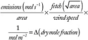
(1)

At sea level the total atmospheric column contains ~356,000 mol m^–2 of air. The lowest 1 km, a typical height of the atmospheric boundary layer, contains ~40,000 mol m^–2 of air at sea level, or ~11 percent of the total atmosphere. In Table B.1 the total column and the boundary layer masses assume the surface to be sea level for each country. At an average wind speed of 5 m s^–1, air moves 430 km in 24 hours, so it takes 4.6 days to traverse a fetch of 2,000 km. Air usually remains in the boundary layer 3-5 days. For longer fetches it becomes increasingly unlikely that all of the emissions remain confined to the boundary layer, and the mole fraction change is then overestimated for those cases.

Table B.1 compares national carbon dioxide (CO₂) emissions and the estimated atmospheric signal for the 20 largest CO₂-emitting nations, which represent more than 80 percent of estimated global emissions. The numbers in the last two columns are typical, but will vary greatly in practice because they are inversely proportional to wind speed. How do the estimates in Table B.1 compare with observations? Based on a very limited number of ¹⁴C measurements of CO₂ in small aircraft off the coast of Cape May and New Hampshire, the average component of CO₂ from recent fossil-fuel combustion is ~3 parts per million (ppm) in the boundary layer.

It is striking to note in Table B.1 how small, relative to background, the mole fraction signals are when averaged over an entire country, and also that the signals for Japan, Germany, and Korea are comparable to those for the two largest emitters: the United States and China. That is due to the higher emissions intensity (per square meter) in the three smaller countries.

Table B.2 presents data from the same 20 countries, for methane (CH₄), nitrous oxide (N₂O), and sulfur hexafluoride (SF₆), estimated in the same way as in Table B.1. When comparing these estimates with U.S. observations from the National Oceanic and Atmospheric Administration network, the estimated

enhancement of greenhouse gas mole fractions is not far from, but on the high side of, observed values for the lowest 1 km, consistent with the fact that over long fetches the emissions tend not to remain confined to the boundary layer. For CH₄, the observed annual average enhancement in the boundary layer of the United States, relative to background values, is 20-60 parts per billion (ppb), with large standard deviation of midday means of 20-30 ppb. For N₂O, these numbers are 0.2-0.4 ppb, and daily standard deviation of 0.3-0.7 ppb; for SF₆, the average enhancement is 0.05-0.2 parts per trillion (ppt), with daily variability of 0.07 to 0.13 ppt. For N₂O, the highest observed enhancement is 0.7 ppb over Iowa, which is indicative of intense regional emissions. The World Meteorological Organization-recommended accuracies for in situ measurements are 2 ppb for CH₄, 0.1 ppb for N₂O, and 0.02 ppt for SF₆.

Table B.3 explores expected enhancements of the CO₂ mole fraction over metropolitan areas. The signal expected to be produced over a single large city relative to its surroundings is comparable to, and in many cases larger than, the average produced by an entire country. Note that the observed average fossil-fuel CO₂ enhancement at the surface in Los Angeles based on ¹⁴C measurements of plants (Figure 4.5) is about five times larger over part of the basin than the number estimated in Table B.3.

The latter is derived with a standard assumption of a steady 5 m s^–1 average wind vector, which would imply that the residence time of air over the metropolitan area would be ~4 hours. Because Los Angeles is surrounded by mountains on three sides, the residence time over the city is much longer.

One gigawatt (GW) corresponds to 8.76 10⁹ kWh yr^–1. Applying the U.S. average 25 mol C kWh^–1, the plant would produce 2.19 10¹¹ mol yr^–1, or 6,900 mol s^–1. If the perpendicular distance across the plume is 1.7 km at some distance downwind, and the wind speed is 5 m s^–1, then 1 second of CO₂ emissions is diluted into 1,700 × 5 m² s^–1 × 3.56 10⁵ mol of air per square meter (full atmospheric column). The number 1.7 km is chosen to correspond to the 3 km² footprint of a single Orbiting Carbon Observatory (OCO) sounding. The CO₂ increase in the total column is then 2.3 ppm.

Significant quantities of CO₂ may one day be captured at large point sources in the utility and industrial sectors and injected into storage sites in the Earth, rather than released to the atmosphere. If this occurs, it will be important to monitor both the quantity of CO₂ that is injected into storage sites and the amount of any CO₂ that leaks from these sites (IPCC, 2005). Leaks from geological sequestration are relatively easy to detect. The emissions are at the surface and are not buoyant like those from a power plant. At night they

will tend to stay at the surface. Assume that the CO₂ from a 1 GW(e) power plant is captured and injected into a well. If 0.1 percent escapes during the injection, there would be a point source of 6.9 mol s^–1 of CO₂. At a point 1 km downstream, with a wind speed of 5 m s^–1 and a plume width of 100 m and plume height of 100 m, the CO₂ enhancement would be 3.3 ppm, causing a ¹⁴C depletion of 0.89 percent. A second scenario is escape from the geological formation into which the CO₂ has been stored. If 0.2 percent of the sequestered CO₂ escapes per year (residence time 500 years), the leak would increase over time as more CO₂ is pumped into the formation. After 1 year the leak rate would be 14 mol s^–1, after 2 years 28 mol s^–1, and so on. In addition, when the escaping CO₂ goes through soil, the CO₂ mole fraction in soil air would become very high, eventually depriving the vegetation of sufficient oxygen in the root zone and leading to plant death, which should be easily detectable.

Dhakal, S., S. Kaneko, and H. Imura, 2003, CO₂ emissions from energy use in East-Asian mega-cities, in Proceedings of the International Workshop on Policy Integration Towards Sustainable Urban Use for Cities in Asia, February 4-5, East-West Center, Honolulu, Hawaii, available at <http://enviroscope.iges.or.jp/ contents/6/index.html>.

IPCC (Intergovernmental Panel on Climate Change), 2005, Carbon Dioxide Capture and Storage, IPCC Special Report, prepared by Working Group III of the Intergovernmental Panel on Climate Change, B. Metz, O. Davidson, H.C. de Coninck, M. Loos, and L.A. Meyer, eds., Cambridge University Press, New York, 442 pp.