
7
FUEL ECONOMY PROJECTIONS
This chapter describes the methods, assumptions, and results of three approaches the committee used to make projections of potential fuel economy levels. The results are ''raw material" for Chapter 8, in which the committee reports its judgments of achievable fuel economy levels.
PROJECTING FUEL ECONOMY LEVELS
Previous Efforts
Projecting future vehicle fuel economy is a risky business. The recent history of such endeavors makes it clear that the chances of being very wrong are very high. In the late 1970s and early 1980s, a number of studies attempted to project fuel economy levels for automobiles and light trucks through 1990. Most of the studies overestimated fleet fuel economy levels by a substantial amount. Estimates for 1990 passenger cars ranged from approximately 30 to 40 miles per gallon (mpg), but the actual fuel economy level was 28 mpg; estimates for light trucks ranged from 20 to 30 mpg, compared with the actual 20 mpg (U.S. Department of Transportation, 1991). The large differences arose mainly because the analysts anticipated continually rising gasoline prices, whereas in the late 1980s gasoline prices were considerably lower in real terms than in the late 1970s.
More recent projections of fuel economy into the early twenty-first century for passenger cars are summarized in Table 7-1. Projections of the fuel economy of the new-car fleet for model year (MY) 2001 range from about 29 to 45 mpg. The wide variation in forecasts is apparently due to such matters as differences in assumptions about what is acceptable to consumers and what is technically possible.
Part of the explanation for the divergence of past projections from subsequent history and for the considerable variation among contemporary projections is that the
TABLE 7-1 Recent Projections of the Average Fuel Economy of Future New Passenger-Car Fleets
|
|
Fleet-Average Fuel Economy (mpg) |
|||
|
Sourcea |
MY 1995-1996 |
MY 2000-2001 |
MY 2005-2006 |
MY 2010 |
|
ACEEEb |
— |
45 |
— |
— |
|
Berger et al.c |
29.5-30.3 |
30.3-32.8 |
— |
— |
|
Bryan billd |
34.3 |
39.5 |
— |
— |
|
Chrysler |
||||
|
Engineering assessmente |
30.1 |
30.9 |
— |
— |
|
Max technology |
— |
34.5 |
— |
— |
|
EEAf |
||||
|
Product plan |
28.3 |
32 |
— |
— |
|
Max technology |
29.1 |
36 |
— |
— |
|
Risk level 1 |
— |
— |
— |
44.8 |
|
Risk level 2 |
— |
— |
— |
54.9 |
|
Risk level 3 |
— |
— |
— |
74.1 |
|
DOEg |
||||
|
Product plan |
32.9 |
36.2 |
— |
— |
|
Cost effective |
— |
38.6 |
— |
— |
|
Max technology |
— |
42.0 |
— |
— |
|
Industryh |
30.2 |
30.6 |
— |
— |
|
Johnston billi |
29.9 |
33.6 |
37 |
— |
|
Ledbetter & Rossj |
— |
40.1-43.8 |
— |
— |
|
Lovinsk |
(no specific time frame) |
(70-100) |
||
|
OTAl |
||||
|
1995 |
29.2-30.0 |
— |
— |
— |
|
2001 |
— |
32.9-38.2 |
— |
— |
|
2005 |
— |
— |
37.1-38.1 |
— |
|
2010 |
— |
— |
— |
45-55 |
|
SRIm |
28.1 |
28.7-30 |
— |
— |
|
a Much of the data in this chart is based on Office of Technology Assessment (OTA, 1991). b Analysts at the American Council for an Energy-Efficient Economy argue that a year-2000 goal of 45 mpg is technologically attainable and cost-effective at today's gasoline prices (Chandler et al., 1988). c Berger et al. (1990) conducted statistical analysis for fuel economy as a function of vehicle attributes: 4.92 to 7.98 percent improvement from 1987 to 1995 and 9.62 to 16.6 percent improvement for 1995-2001. d Sen. Richard Bryan's bill (S.279): 20 percent over 1988 by 1996; 40 percent by 2001. e Bussmann (1990) indicates 7.1 percent gain from 1989-1995 and 2.8 percent from 1995-2000. Under maximum technology case, 14.6 percent gain from 1995 to 2000 (see OTA, 1991:Table 7-2). f Energy and Environmental Analysis, Inc. Estimates are for the domestic fleet only: risk level 1 refers to technologies most agree are likely to be commercialized; level 2 is technology about which opinion is sharply divided; level 3 is technology considered esoteric by most, but within the realm of possibility (OTA, 1991:58). g U.S. Department of Energy: product plan, 17.1 percent increase from 1987-1995, and 9.9 percent increase from 1995-2000. Cost-effective assumption, 17.2 percent increase from 1995-2000; maximum technology, 27.6 percent from 1995-2000 (see OTA, 1991:Table 7-1). h Estimates presented by the automotive companies at the committee's July 1991 workshop (see Appendix F) were on the order of a 10 percent increase from 1990 to 2001. Toyota indicated an 11 percent increase by 2001; Chrysler indicated a 17 percent increase for small cars, 19 percent for midsize, and 6 percent for large cars from 1990-2001; Honda indicated 10 to 11 percent for 1990-2001 (without considering emissions and safety requirements, 14 to 15 percent); General Motors indicated 1 to 2 mpg above 24 mpg would be cost-effective for a gasoline price of $1.34/gallon in 2000 for the Buick Park Avenue; Nissan reported 10.6 percent from 1990-2000; Mitsubishi reported 8 percent. OTA (1991:Table 7-3) reports a 7.6 percent improvement from 1989 to 1995 for the domestic industry. i Sen. Bennett Johnston's bill (S.1220): 7.5 percent increase from 1990-1996; 20.9 percent from 1990-2001; 31.8 percent from 1990-2006. The 1996 standard involves nearly full market penetration of fuel-saving technologies and substantial penetration by the two-stroke engine. Light-truck corporate average fuel economy (CAFE) levels are 22.0, 24.0, and 26.6 mpg for 1996, 2000, and 2006, respectively, for the combined domestic and import fleets. j Ledbetter and Ross (1990) use a variation on Energy and Environmental Analysis, Inc.'s analysis for OTA (1991) that is based on more optimistic assumptions. k Amory Lovins at the committee's July 1991 workshop (see Appendix F) indicated large increases with reduced costs but no specific time frame. l OTA (1991) estimates range from optimistic to pessimistic values depending on the scenario envisioned. From 1995 to 2001, the scenarios range from a fairly optimistic "business as usual" at the low end to a regulatory, technology-forcing scenario at the high end. From 2005 on, regulation-driven scenarios are envisioned both for the low and high estimates in 2006 and 2010. m SRI (1991). |
projections have entirely different foundations. Some projections reflect what the analysts would prefer to have happen and vary substantially in the degree of recognition of practical constraints or, alternatively, future opportunities. Other projections represent the analysts' best estimates of what will happen, not necessarily what they prefer to have happen. The analysts may attempt to account for specific anticipated changes that bear on fuel economy projections, or they may assume that change of some unspecified nature will occur with the passage of time. Still other projections attempt to establish the limits of what is possible, with little or no reference to the degree to which the possible is feasible. Finally, some projections attempt to take into account the possibility of radical change in technology, in values, or in the political, economic, or natural conditions that impinge on fuel economy. In light of these facts, the differences among the various estimates are not surprising.
Overview of the Projection Methods
The committee used three types of quantitative projections: historical trend projection; "best-in-class" (BIC) analysis; and the technology-penetration, or "shopping cart," approach.
Historical trend projections are based on the assumption that the past trend in some measure of overall performance can be extended reliably into the future. This study projects recent experience with the fuel economy of the new vehicle fleet to MY 2006. It also projects a weight-adjusted measure of the technical efficiency of the new vehicle fleet, namely ton-miles per gallon (ton-mpg), over the same period.
Best-in-class analysis is a hybrid approach. This type of analysis assumes that the fuel economy of the typical new vehicle at some unspecified future date will be equal to that of an exemplary vehicle or group of vehicles already in the fleet.
The technology-penetration, or shopping cart, approach attempts to locate the limits of possibility, subject to certain constraints, by assuming that specific, well-characterized, fuel-saving technologies will be adopted in a larger proportion of all vehicles than they are today. Unlike the trend-projection and BIC methods, the shopping cart approach provides the basis for an explicit projection of costs.
Assumptions Common to All Projections
Several assumptions underlie all of the fuel economy projections in this study. First, such amenities as air-conditioning, automatic transmissions, high ride quality, and brisk acceleration are assumed to continue at current levels. For example, horsepower-to-weight ratios (a performance measure) are not changed in most of the projections from the base MY 1990 levels;1 technologies having potentially serious customer-acceptance problems, such as engine-off at idle, are excluded from the shopping cart
analysis; and MY 1990 market share levels are kept constant for certain technologies that have important implications for consumers.2
A second assumption is that there will be a "normal" rate of technological progress in fuel economy improvement between now and 2006. Higher levels of fuel economy will be possible in the future than are possible today, at reasonable costs, but radical breakthroughs in technology are assumed not to occur.
Third, it is assumed that the means used to improve fuel economy will be consistent with compliance with the Tier I emissions standards of the 1990 amendments to the Clean Air Act, as discussed in Chapter 4. This constraint is reflected in the assumption that there will be an overall fuel economy penalty of 1 percent due to the added weight of emissions-control equipment. No other impact on vehicle performance is assumed to result from compliance with new emissions standards. It is further assumed that automobile makers will conform with expected future safety standards, as discussed in Chapter 3, with a consequent fuel economy penalty of 2 percent for the added weight likely to be necessary to meet those requirements.
Fourth, it is assumed that there will be no shifts of consumer preferences among the size classes or from automobiles to light trucks. The committee uses the Environmental Protection Agency's (EPA's) vehicle classification system of nine passenger-car and six light-truck classes. Projections were made for the four largest selling classes of cars (subcompacts, compacts, midsize, and large) and trucks (small pickups, large pickups, small vans, and small utility vehicles). These classes account for 92 and 88 percent of car and light-truck sales, respectively (Heavenrich et al., 1991).3
HISTORICAL TREND PROJECTIONS
Although extrapolation of past trends may not always accurately reveal the future, there is no reason to believe that extrapolation of fuel economy trends is inevitably unreliable. Indeed, trend projection has the advantage of being inherently temporal and, thus, able to suggest how rapidly improvements might be achieved. The method provides a crude but revealing indicator of possible fuel economy gains.
As discussed in Chapter 1, fuel economy gains averaging 1 to 1.5 mpg per year were achieved during the 1970s as a result of vehicle downsizing and downweighting associated with the conversion of most of the fleet to front-wheel drive, the development of the three-way catalyst, and other technological improvements. During the mid-1980s, vehicle weights stabilized, and technological improvements resulted in
a slower rate of fuel economy increases (0.4 to 0.5 mpg per year). From the late 1980s to the present, acceleration performance was enhanced and vehicle weights increased slightly, which resulted in a small reduction in fleet fuel economy.
The historical trend projections of fuel economy were made by linear extrapolation of trends in two measures—mpg and ton-mpg—using the method of linear least squares to fit trend lines for the 16-year base period, 1975-1991, as illustrated in Figures 7-1 and 7-2.4 Other projection lines could be obtained by fitting subsets of the historical data. For example, during the early part of the base period, rising fuel prices, anticipation of growing fuel shortages, and the need to meet future fuel economy requirements motivated rapid improvement of fuel economy. Projecting the rate of progress during that period would lead to very high fuel economy forecasts for MY 2006.5 On the other hand, during later parts of the period, compliance with CAFE requirements may have been the only major reason for manufacturers to pay attention to fuel economy, and progress slowed. Thus, projecting the experience of the past decade would lead to a forecast of quite small improvements. The committee recognizes that fleet-average fuel economy closely followed the mandated fuel economy standards over the 1978-1991 period and does not fit a straight line particularly well. Nonetheless, in the absence of any obviously preferable choice, the committee projected the straight lines over the entire period to estimate future fuel economy progress.
The trend-based extrapolation results for cars and light trucks are summarized in Tables 7-2 and 7-3. The mpg-based MY 2006 projections for the new car and truck fleets were obtained from the linear extrapolations beyond MY 1991. (Each MY 2006 value was reduced by 3 percent to account for the fuel economy penalty associated with meeting anticipated safety and emissions requirements.) The mpg-based MY 2001 projections for the new car and truck fleets were then obtained by linear interpolation between the actual MY 1991 level and the adjusted MY 2006 projections. The ton-mpg projections for all cars and all trucks were obtained similarly, assuming that the average weight of all cars and trucks in MY 2001 and MY 2006 remain at the reported MY 1991 values. Projections for each size class of cars and trucks for MY 2001 and MY 2006 were then obtained by applying the percentage increases that apply to each fleet to the reported MY 1991 values for each size class.
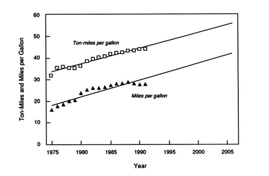
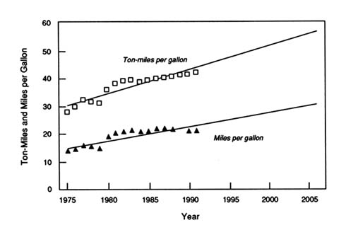
TABLE 7-2 Trend Projections of Fuel Economy of New Passenger Cars
|
|
Fuel Economy (mpg) |
|
|
Size Class and Model Year |
Based on MPG Trends for 1975-1991 |
Based on Ton-MPG Trends for 1975-1991 |
|
Car fleet |
||
|
1991 |
27.8 |
27.8 |
|
2001 |
34.9 |
32.3 |
|
2006 |
38.5 |
34.5 |
|
Subcompact cars |
||
|
1991 |
31.2 |
31.2 |
|
2001 |
39.2 |
36.2 |
|
2006 |
43.2 |
38.7 |
|
Compact cars |
||
|
1991 |
29.2 |
29.2 |
|
2001 |
36.7 |
33.9 |
|
2006 |
40.4 |
36.2 |
|
Midsize cars |
||
|
1991 |
25.8 |
25.8 |
|
2001 |
32.4 |
29.9 |
|
2006 |
35.7 |
32.0 |
|
Large cars |
||
|
1991 |
23.7 |
23.7 |
|
2001 |
29.8 |
27.5 |
|
2006 |
32.8 |
29.4 |
|
NOTE: Projections for MY 2006 have been adjusted downward by 3 percent to account for the fuel economy impact of safety and emissions (Tier I) standards. Data for 1991 are from Heavenrich et al. (1991). These projections are considered as input to the committee's estimates reported in Chapter 8. |
||
TABLE 7-3 Trend Projections of Fuel Economy of New Light Trucks
|
|
Fuel Economy (mpg) |
|
|
Size Class and Model Year |
Based on MPG Trends for 1975-1991 |
Based on Ton-MPG Trends for 1975-1991 |
|
Light truck fleet |
||
|
1991 |
20.8 |
20.8 |
|
2001 |
25.2 |
24.8 |
|
2006 |
27.5 |
26.8 |
|
Small utility trucks |
||
|
1991 |
21.2 |
21.2 |
|
2001 |
25.7 |
25.2 |
|
2006 |
28.0 |
27.3 |
|
Small vans |
||
|
1991 |
22.8 |
22.8 |
|
2001 |
27.7 |
27.2 |
|
2006 |
30.1 |
29.3 |
|
Small pickups |
||
|
1991 |
25.2 |
25.2 |
|
2001 |
30.6 |
30.0 |
|
2006 |
33.3 |
32.4 |
|
Large pickups |
||
|
1991 |
19.5 |
19.5 |
|
2001 |
23.7 |
23.2 |
|
2006 |
25.8 |
25.1 |
|
NOTE: Projections for MY 2006 have been adjusted downward by 3 percent to account for the fuel economy impact of safety and emissions (Tier I) standards. Data for 1991 are from Heavenrich et al. (1991). These projections are considered as input to the committee's estimates reported in Chapter 8. |
||
The mpg-based projections indicate that the MY 2006 fleet-average fuel economy might increase by about 38 percent for passenger cars and by about 32 percent for light trucks above MY 1991. The ton-mpg-based projections indicate that the MY 2006 fleet-average fuel economy might increase by about 24 percent for cars and 29 percent for trucks above MY 1991. For passenger cars, the fuel economy projections based on mpg are higher than those based on ton-mpg, in part because future weight reductions are assumed not to occur in the ton-mpg projections, whereas weight reduction is implicit in the mpg projections. The ton-mpg projections would have been higher had future weight reductions been taken into account. For light trucks, projections based on the two methods are nearly identical because weight reduction has not historically been a significant factor in their fuel economy improvement.
BEST-IN-CLASS (BIC) PROJECTIONS
The BIC method is based on the assumption that the average fuel economy of each vehicle class could eventually reach the level of the best vehicle, or several top vehicles, currently in that class. The method implicitly assumes that the cost of achieving the BIC fuel economy level for an entire class would be no greater than the costs of lost consumer satisfaction and manufacturers' profits as a result of restricting consumer choices to the BIC vehicle(s) or ones of similar design. Of course, if technology were to improve, the fuel economy performance of the BIC vehicle(s) might be achieved by vehicles with a wider range of amenities in the future.
There is an implicit time period for achieving the BIC fuel economy level: the time it would take to redesign, produce, and sell vehicles in each class such that the class-average fuel economy would be equal to the fuel economy of the current BIC vehicles. Platform designs, as noted earlier, are essentially established through MY 1995, but the BIC levels estimated in this report should, according to the discussion in Chapter 5, be achievable by manufacturers by MY 2006 without undue disruption to normal product cycles.
The EPA annually carries out BIC fuel economy analyses for the fleet and each weight class (Heavenrich et al., 1991). It ranks individual configurations (a car line with a specific engine and transmission combination) without regard to sales volume, and it identifies the BIC vehicle, the five BIC vehicles, and the top dozen vehicles within each weight class (the weight classes differ from the volume-based size classes used throughout this report).6
The EPA also ranks all configurations according to their fuel economy and identifies the average fuel economy of various percentile groups. Figure 7-3 shows the trends in fuel economy for each percentile group. It shows that the average passenger car in MY 1986 through MY 1991 achieved a fuel economy (28 mpg) about equal to that of the ninety-fifth percentile car in MY 1975. Roughly 10 years were required to accomplish that change. In MY 1991, the ninety-fifth percentile passenger car had a fuel economy of about 45 mpg. This chart makes clear that the very top-ranked cars (in mpg) have become decreasingly typical of the rest of the fleet over time.
In this study the BIC vehicle(s) are chosen using an approach different from EPA's. Vehicles are defined by car line, not by configuration, and classed by interior volume (cars) or size and function (trucks), not by weight.7 The BIC vehicles are those in the top rank that together account for at least 5 percent of class sales. The BIC fuel economy for each class is calculated as the sales-weighted harmonic average fuel economy (see Chapter 9) of the BIC car lines, reduced by 3 percent for the effects of safety and emissions standards.
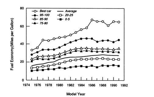
FIGURE 7-3 New passenger-car fuel economy by percentile group.
SOURCE: Heavenrich et al. (1991).
Tables 7-4 and 7-5 show the results of the BIC analysis based on MY 1990 vehicles. For passenger cars, this analysis yields BIC fuel economy levels that are 50 percent above the current class average for subcompacts, about 13 percent for compacts, 8 percent for midsize cars, and 3 percent for large cars. There is a wide range of fuel economy values among the BIC vehicles in the subcompact class, a market segment in which fuel economy is considered an especially important attribute by many car buyers. Some manufacturers introduce cars in this class that are intended to compete for the title of the most fuel-efficient car sold in the United States. As a consequence of that competition, the most efficient subcompact car tends to have fewer of the other attributes most valued by consumers, even for its size class. As a result, the BIC analysis may exaggerate the potential fuel economy improvement for smaller cars. In contrast, in the large car class there is little variation in fuel economy among the BIC car lines. To the extent that there is no competition for the most efficient car in the other size classes, the BIC analysis may underestimate potential fuel economy gains.
The BIC fuel economy levels for the four light-truck classes shown in Table 7-5 represent modest gains for the small pickup and compact van classes (on the order of 5 percent), but substantial gains for large pickups and small utility vehicles (38 percent and 40 percent, respectively). This result best illustrates a weakness of the BIC approach applied at the vehicle-class level—it is sensitive to a few extreme cases and to the precise definitions of the classes. For example, the BIC large pickup truck is the Toyota, which has a fuel economy rating of 27.1 mpg, whereas the top-ranked domestically manufactured large pickup is the Dodge Power Ram 50, which has a fuel economy rating of 23.4 mpg, 15 percent lower. However, large pickups manufactured in the United States are considerably larger than the imported large pickups that rank at the top of the fuel economy scale, even though the definition of the large pickup class is broad enough to include both. Thus, the committee believes that the BIC method, as applied here to light trucks, gives only a general indication of fuel economy potential by class.
TECHNOLOGY-PENETRATION OR SHOPPING CART PROJECTIONS
Method and Assumptions
The technology-penetration projection method is based on an explicit consideration of the potential fuel economy contributions of specific, well-established technologies. It is referred to here as the "shopping cart" approach because it allows selection, one-by-one, of a set of fuel economy technologies, followed by a calculation of their contributions to vehicle fuel economy and cost. The shopping cart approach, as used by the committee, assumes that each technology will achieve its maximum possible market penetration—up to 100 percent where appropriate—and that each technology will be fully deployed before the next most cost-effective technology's market share increases above its base line.
TABLE 7-4 Best-In-Class (BIC) Fuel Economy, MY 1990 Passenger Cars
|
Size Class and Car Line |
Market Share In Size Class |
Fuel Economy (mpg) |
|
Subcompact |
||
|
Chevrolet Sprint/Geo Metro |
0.026 |
52.6 |
|
Geo Metro (domestic) |
0.013 |
52.0 |
|
Daihatsu |
0.006 |
43.1 |
|
Subaru Justy |
0.008 |
39.3 |
|
BIC |
0.052 |
47.2 |
|
Compact |
||
|
Isuzu Stylus |
0.000a |
35.4 |
|
Ford Escort |
0.088 |
34.4 |
|
BIC |
0.088 |
33.4 |
|
Midsize |
||
|
Dodge Aries/Plymouth Reliant |
0.005 |
30.0 |
|
Mazda 626 |
0.011 |
29.6 |
|
Mazda MX6 |
0.000b |
29.1 |
|
Chevrolet Corsica |
0.068 |
28.3 |
|
BIC |
0.084 |
27.7 |
|
Large |
||
|
Buick Electra/Park Ave. |
0.044 |
25.0 |
|
Buick LaSabre |
0.119 |
25.0c |
|
BIC |
0.163 |
24.3 |
|
NOTE: The car lines listed are those in the top rank for that class that together account for at least 5 percent of class sales. The BIC fuel economy for each class is the sales-weighted harmonic average fuel economy of these car lines adjusted downward by 3 percent to account for safety and emissions (Tier I) standards. a 326 cars sold. b 249 cars sold. c The next three large cars in rank order also rated 25.0 mpg: Oldsmobile 88, Oldsmobile 98, and Pontiac Bonneville. SOURCE: Data are from Williams and Hu (1991): Tables 16-19. |
||
TABLE 7-5 Best-In-Class Fuel Economy, MY 1990 Light Trucks
The committee used the shopping cart approach to construct curves relating fuel economy improvement to cost. In doing so, it assumed that the individual technologies are adopted in the order of decreasing cost-effectiveness (mpg per dollar) and that their incremental costs and fuel economy contributions are independent of market share.8 The base year is MY 1990. Since the method uses only proven technologies, it assumes that the technologies can be implemented by manufacturers in the normal process of replacing manufacturing equipment, that is, in 15 years or less. Thus, estimates can be made of the costs of improving fuel economy to any particular level, so that curves of cumulative cost versus fuel economy improvement can be generated. Although these cost curves must be interpreted with care, for reasons pointed out below, they are quite useful for indicating the general tendencies for costs and risk to increase as higher levels of fuel economy are pursued.
As each technology is added to vehicles in a size class, the average increase in fuel economy for a car or light truck in the class is computed by multiplying an estimate of the percentage improvement in fuel economy achievable in a single vehicle by the change in market share for the technology from the MY 1990 level to the maximum possible for the class, and then multiplying the result by the base-year average fuel economy for the class. The average increase in cost for the size class due to increased use of each technology is computed by multiplying the average cost increase by the average market share change, both in the class. For the set of technologies applicable to a size class, summing the average fuel economy gains and average costs yields estimates of aggregate fuel economy gains and costs for the size class. The average gain in fuel economy is then added to the average fuel economy for the size class in the base year (3 percent having been subtracted from the base-year fuel economy to account for the effects of safety and emissions technology) to obtain an estimate of the fuel economy potential of the size class. (The method is detailed in Appendix E.)
The shopping cart estimates involve several other assumptions:
-
Only proven technologies are included. No allowance was explicitly made for the development of new technologies or for the refinement of existing ones. This conservatism gives some assurance that the fuel economy gain could actually be achieved.
-
For the main shopping cart analysis, vehicle performance was held constant at MY 1990 levels. (The effect of reducing horsepower/weight ratios to those of new MY 1987 vehicles was also examined to explore the kinds of trade-offs that might be made.)
-
The analysis included downsizing associated with conversion of most of the remaining rear-wheel drive vehicles to front-wheel drive, as well as a 10 percent weight reduction through materials substitution.9
-
The maximum market shares for each technology for each vehicle type were assumed to be 100 percent unless there were compelling reasons to limit market penetration.10
-
Positive and negative synergistic effects among technologies were neglected, and thus, individual percentage improvements for different technologies were assumed to be additive.11
Data
The shopping cart algorithm requires several key inputs. The MY 1990 base-year composite fuel economy rating used for each car and light-truck class is that reported by Heavenrich et al. (1991). Data on the characteristics, fuel economy contributions, costs, and market shares of each technology were obtained from a variety of sources. The principal sources are reports compiled by SRI International for the Motor Vehicle Manufacturers Association (SRI, 1991) and by Energy and Environmental Analysis (EEA), Inc., a U.S. Department of Energy contractor (EEA, 1991a,b, and personal communication, October 2, 1991). Details of the data sources are provided in Appendix B. As discussed below and in Appendix B, there are substantial differences among these reports, especially regarding costs.12
The committee compiled a list of available fuel economy technologies applicable to conventional automobiles and light trucks based on information provided by automobile manufacturers and others who made presentations to the committee (see
Table 2-2). The list includes the most important fuel economy technologies that, in the committee's view, satisfy the criteria of being in mass production and not degrading consumer satisfaction. Appendix B includes descriptions of the selected technologies and estimates of their fuel economy improvement potentials and costs. The list is generally consistent with available published studies, such as that of OTA (1991), and it is nearly identical to the list provided to the committee by the Ford Motor Company.13 However, it is shorter, for example, than the list contained in the 1991 SRI study (Tables 11 and 12), and it excludes certain technologies (such as "friction reduction II") included in some studies by EEA (1990).14
Technologies are grouped into those that pertain to (1) the engine generally (internal friction, accessory loads, thermodynamic efficiency), (2) fuel systems, (3) valve train, (4) number of cylinders, (5) transmission technologies, and (6) technologies that affect power demands, such as rolling resistance, aerodynamics, and vehicle weight. These groups of technologies are mutually exclusive (e.g., 5-speed manual and 4-speed automatic transmissions) or mutually compatible (e.g., improved aerodynamics and advanced tires). Within mutually exclusive groups, market shares must sum to 100 percent; within mutually compatible groups, market shares are independent and each could be as high as 100 percent.
The EEA and SRI studies deal with passenger cars and generally exclude light trucks (EEA, 1988). However, nearly all of the technologies applicable to automobiles are applicable to light trucks, with a few exceptions and adjustments. For example, front-wheel drive is not likely to be as widely applicable to light trucks, in part because rear-wheel drive allows greater towing capacity. On the other hand, diesel engines are not included in the passenger-car options, but they are included for light trucks, for which problems of consumer acceptance and emissions standards are relatively less severe in certain market segments.
The costs of fuel economy improvement proved to be the most controversial factor in the analysis. Disagreements over costs have partly to do with valuing sunk investments. For example, one should compare the costs of two alternative new technologies by taking into account total capital costs, variable material and labor costs, and all overhead, burdens, and profit margins for each. The cost difference between the two would yield the expected difference in retail price equivalent (RPE).15 On the other hand, in considering the cost implications of replacing a production facility for an existing technology with one for a new technology, one would compare the full capital
costs of the facility for the new technology with the lower level of capital spending required to maintain the manufacturing capability for the existing technology.16 In such a case, the new technology would look far more expensive than the continuation of the existing technology. This difference is important because it relates to the timing of regulatory standards. To the extent that standards require the premature replacement of useful capital, their cost will be higher than if they allowed new fuel economy technology to be introduced as part of a "normal" capital turnover process.
The committee believes that part of the differences between the cost estimates provided by SRI and EEA can be explained by the timing of the required investments. SRI developed two sets of cost estimates, one for MY 1995 and another for MY 2001. (The estimates for MY 2001 are used in this study.) The estimates purportedly reflect the incremental costs that domestic manufacturers would face in making technology changes by 2001, given their current product plans. That is, the capital cost of a technology a manufacturer already has in production will be relatively lower than that of a new technology, for which production facilities and equipment may have to be purchased. On the other hand, the EEA analysis assumes that full capital costs must be borne for the baseline as well as the new technology, so that the difference in costs is likely to be smaller. The EEA estimates might be construed as reflecting the long-run RPE of a fuel economy technology in comparison to the RPE of a "base" technology. In contrast, SRI's estimates might be seen as short-run RPEs, in that they reflect the costs of premature abandonment of productive capital investments.
Results
Using the shopping cart approach, the committee developed two projections of fuel economy and costs for each vehicle size class. The projections rely on the committee's adaptation of SRI's and EEA's technology-specific estimates of fuel economy improvement potentials and costs and on the committee's assumptions regarding maximum market shares. The committee's projections are called Case A and Case B, respectively. Cases A and B are intended to indicate a range of possibilities, from relatively high-cost, moderate fuel economy improvements (Case A, based heavily on SRI data) to relatively low-cost, greater fuel economy gains (Case B, based heavily on EEA data). The resulting projections differ significantly from earlier ones by SRI and EEA because of the committee's market share assumptions and its adjustment of the SRI and EEA data in certain cases.
Figures 7-4 through 7-11 illustrate the results of the shopping cart analysis for the various passenger-car and light-truck classes.17 The curves for Case A and Case B for


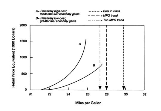
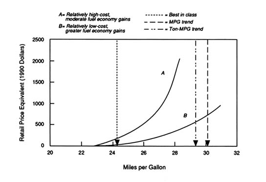

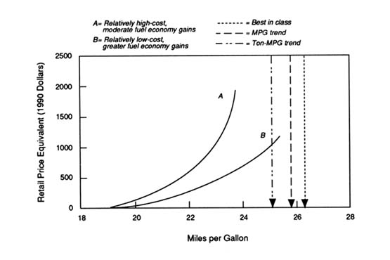
each class exhibit the expected concave upward shapes that result from adding technologies to the MY 1990 baseline in the order of their decreasing cost-effectiveness. For each vehicle class, the costs at a given level of fuel economy differ quite substantially for the two cases, but the end points (the levels of fuel economy at which the potential contributions of all proven technologies on the list are exhausted) differ much less. Put another way, the committee's shopping cart analysis yields cost projections that are inherently much more uncertain than the fuel economy projections. Finally, it should be noted that time is not a variable in Figures 7-4 through 7-11 and that the analysis is not intended to suggest that the time path of adoption of new fuel economy technologies would follow the curves of Case A or Case B. What the curves do represent is the locus of ''least-cost" combinations of technologies that would give a class-average fuel economy of a particular level, subject to the many assumptions of the method.
To estimate the potential impact of performance reductions on the end points of the shopping cart curves, the committee increased the end-point fuel economy for each vehicle class by a percentage reflecting the changes associated with returning the MY 1990 horsepower/weight ratio for each class to its MY 1987 value. The results, summarized in Table 7-6, suggest that such performance reductions could facilitate an increase in end-point fuel economy ranging from 1 to 2 mpg for cars, and from 0 to 1.6 mpg for light trucks. The effects of performance reduction for each class are essentially the same whether based on Case A or Case B.
As seen by examining Figures 7-4 through 7-11, the various projection methods do not provide entirely consistent results. Sometimes the trend projection gives the highest fuel economy estimate, and sometimes the best-in-class approach suggests the highest level. While there is some tendency for the various projections to cluster, the methods do not provide clear and uniform estimates of future levels of automobile and light-truck fuel economy. The results are revealing, but they do not eliminate the need for judgment.
CONCLUSIONS
-
Three very different methods were used to project the future fuel economy levels for passenger cars and light trucks. Each method exemplifies a different view of the problem and each yields different projections of the potential for fuel economy improvement by vehicle class. None of the projections in this chapter reflects the views of the committee regarding practically achievable levels of fuel economy, which are discussed in the next chapter.
-
None of the projection methods predicts what will happen or what ought to happen. Each gives a different view of what could be achieved and provides a different insight about the implications of increased fuel economy.
TABLE 7-6 Effect of Performance Reduction on Projected Fuel Economy Levels
|
|
|
Projected End-Point Fuel Economyb (mpg) |
Increase in Fuel Economy Due to Performance Reductionc (mpg) |
||
|
Vehicle Class |
Performance Reductiona (percent) |
Case A |
Case B |
Case A |
Case B |
|
Cars |
|||||
|
Subcompact |
12.7 |
38.5 |
40.7 |
1.8 |
1.9 |
|
Compact |
13.8 |
35.3 |
37.2 |
1.8 |
1.9 |
|
Midsize |
11.9 |
31.4 |
34.1 |
1.4 |
1.5 |
|
Large |
8.6 |
29.0 |
31.9 |
0.9 |
1.0 |
|
Light trucks |
|||||
|
Small pickups |
13.5 |
31.1 |
32.9 |
1.5 |
1.6 |
|
Small vans |
0.0 |
28.3 |
30.9 |
0.0 |
0.0 |
|
Large pickups |
12.7 |
23.8 |
25.4 |
1.1 |
1.2 |
|
Small utility vehicles |
14.3 |
25.9 |
27.5 |
1.3 |
1.4 |
|
a Performance reduction is measured by changes in class-average horsepower/weight ratios from MY 1990 to MY 1987 levels from Heavenrich et al. (1991). b Fuel economy projections are based on the shopping cart approach keeping vehicle performance fixed at MY 1990 levels. c Each 1 percent decrease in the horsepower/weight ratio is estimated to result in a 0.38 percent increase in fuel economy, based on estimates of the effect of engine displacement on fuel economy (EEA, 1991a). |
|||||
-
Each method provides an estimate of what might be achieved 10 to 15 years into the future under normal rates of product redesign, capital investment, and vehicle sales. All three methods indicate that substantial fuel economy improvements may be technically possible.
-
The technology-penetration method suggests that further accelerating the process of fuel economy increase could be quite expensive.
-
The BIC-based projections of the percentage improvements in fuel economy vary greatly from class to class, which suggests that the method may not be reliable at the class level.
None of the projections offers proof of technical potential. Together, however, they increase confidence that substantial fuel economy improvements could be achieved over the next 15 years without compromising the functionality of light-duty vehicles. There will be a price to pay, however, and some trade-offs will be required. Whether attaining such levels of fuel economy is likely to be worth the cost to consumers, manufacturers, or the nation is the subject of the following chapter.
REFERENCES
Berger, J.O., M.H. Smith, and R.W. Andrews. 1990. A system for estimating fuel economy potential due to technology improvements. Paper presented at workshop of the Committee on Fuel Economy of Automobiles and Light Trucks, Irvine, Calif., July 8-12. University of Michigan, Ann Arbor.
Bussmann, W.V. 1990. Potential Gains in Fuel Economy: A Statistical Analysis of Technologies Embodied in Model Year 1988 and 1989 Cars. Chrysler Corporation, Detroit, Mich.
Chandler, W.U., H.S. Geller, and M. Ledbetter. 1988. Energy Efficiency: A New Agenda. Washington, D.C.: American Council for an Energy-Efficient Economy.
Energy and Environmental Analysis (EEA), Inc. 1988. Light Duty Truck Fuel Economy: Review and Projections, 1980-1995. Prepared for U.S. Department of Energy, Office of Policy, Planning and Analysis. Arlington, Va.
Energy and Environmental Analysis (EEA), Inc. 1990. Analysis of the Fuel Economy Boundary for 2010 and Comparison of Prototypes. Draft final report. Prepared for Martin Marietta, Energy Systems, Oak Ridge, Tenn. Arlington, Va.
Energy and Environmental Analysis (EEA), Inc. 1991a. Fuel economy technology benefits. Presented to the Technology Subgroup, Committee on Fuel Economy of Automobiles and Light Trucks, Detroit, Mich., July 31.
Energy and Environment Analysis (EEA), Inc. 1991b. Documentation of Attributes of Technologies to Improve Automotive Fuel Economy. Prepared for Martin Marietta, Energy Systems, Oak Ridge, Tenn. Arlington, Va.
Heavenrich, R.M., J.D. Murrell, and K.H. Hellman. 1991. Light-duty Automotive Technology and Fuel Economy Trends Through 1991. Control Technology and Applications Branch, EPA/AA/CTAB 91-02. Ann Arbor, Mich.: U.S. Environmental Protection Agency.
Ledbetter, M., and M. Ross. 1990. Supply curves of conserved energy for automobiles. Proceedings of the 25th Intersociety Energy Conservation Engineering Conference. New York: American Institute of Chemical Engineers.
Office of Technology Assessment (OTA), U.S. Congress. 1991. Improving Automobile Fuel Economy: New Standards, New Approaches. Washington, D.C.: U.S. Government Printing Office.
Samples, D.K., and R.C. Wiquist. 1978. TFC/IW. Presented at the International Fuels and Lubricants Meeting, Royal York, Toronto, November 13-16. SAE Technical Paper Series 780937. Warrendale, Pa.: Society of Automotive Engineers.
SRI International. 1991. Potential for Improved Fuel Economy in Passenger Cars and Light Trucks. Prepared for Motor Vehicle Manufacturers Association. Menlo Park, Calif.
U.S. Department of Transportation. 1991. Briefing Book on the United States Motor Vehicle Industry and Market, Version 1. Cambridge, Mass.: John A. Volpe National Transportation Systems Center.
Williams, L.S., and P.S. Hu. 1991. Highway Vehicle MPG and Market Shares Report. ORNL-6672. Tenn.: Oak Ridge National Laboratory.


