
4
Haze Formation and Visibility Impairment
To develop an effective strategy for ameliorating the effects of human activities on visibility, the complex processes that form haze and impair visibility must be understood. The primary visibility attributes—light extinction, contrast, discoloration, and visual range—can be quantitatively measured, and despite some limitations in knowledge about visibility, changes in those attributes can be related to changes in the chemical and physical properties of the atmosphere.
This chapter presents the current scientific understanding of the processes involved in haze formation and visibility impairment. In this chapter we discuss
-
Some of the fundamental factors that relate to haze and visibility;
-
The role of meteorological processes in haze formation;
-
Experimental strategies for monitoring visibility;
-
The modeling of the relationship between aerosol properties and visibility;
-
Issues related to quality assurance and quality control.
The measurement techniques used to characterize the components that affect visibility are reviewed in Appendices A and B; Appendix B discusses techniques used to relate the human perception of visibility degradation to physical measurements.
FUNDAMENTALS OF VISIBILITY AND RELATED MEASUREMENTS
Fundamental Processes in Visibility
If an observer is to see an object, light from that object must reach the observer's eye. The perceived visual character of the image depends on the light emitted from or reflected by the object and on the subsequent interaction of that light with the atmosphere. When an observer views a distant object, the light reaching the observer is weakened by two processes: absorption of energy or scattering by gases or particles in the atmosphere. These two processes are referred to collectively as extinction and are depicted in Figure 4-1.
Transmitted light is not the primary factor that determines visibility. The visibility of a distant object also is affected by light from extraneous sources (e.g., sun, sky, and ground) that is scattered toward the observer by the atmosphere (Figure 4-1). This extraneous light is referred to as air light. The air light behind an object provides backlighting and causes the object to stand out in silhouette (iv in Figure 4-1); the air light between the observer and an object tends to reduce the contrast of the object and to mute its colors (v in Figure 4-1).
Air light can be an important element of a view; it can have a positive as well as a negative effect on perception. The appearance of the daytime sky is due the scattering of sunlight by gases and particles in the atmosphere. If there were no scattering (or if there were no atmosphere), the daytime sky would be black, allowing the stars to be seen during the day. Air light also provides diffuse light to the surface below; without air light, objects viewed on Earth would have the deep shadow effects seen in photographs of the Moon.
Haze affects the quality and quantity of air light because absorption and scattering are wavelength dependent. That dependence accounts for the deep blue color of the sky in pristine areas, as well as the gray color of smog. Air light is proportional to extinction and, like extinction, depends on particle concentrations. Unlike extinction, air light also depends on viewing angle; particles scatter preferentially in forward directions, so that haze tends to appear brighter in the direction of the sun.
The extinction coefficient, bext, is a key measure of atmospheric trans-

FIGURE 4-1 Elements of daytime visibility. The atmosphere modifies an observer's view of a distant object, in this case a tree illuminated by the sun. The paths illustrate: (i) light from the target that reaches the observer; (ii) light from the target that is scattered out of the observer's line of sight; (iii) light absorbed by gases or particles in the atmosphere; (iv, v) light from the sun or sky that is scattered by the intervening atmosphere into the observer's line of sight; process iv causes the object to stand out in silhouette while v reduces the contrast of the object. Source: EPA, 1979.
parency and is the measure most directly related to the composition of the atmosphere. It is a measure of the fraction of light energy dE lost from a collimated beam of energy E in traversing a unit thickness of atmosphere dx: dE =-bextEdx. The extinction coefficient has dimensions of inverse length (e.g., m-1). The extinction coefficient comprises four additive components:
where
bsg = light scattering by gas molecules. Gas scattering is almost entirely attributable to oxygen and nitrogen molecules in the air and often is referred to as Rayleigh or natural "blue-sky" scatter. It is essentially unaffected by pollutant gases.
bag = light absorption by gases. Nitrogen dioxide (NO2) is the only common atmospheric gaseous species that significantly absorbs light.
bsp = light scattering by particles. This scattering usually is dominated by fine particles, because particles 0.1–1.0 µm have the greatest scattering efficiency. Many pollutant airborne particles are in this size range.
bap = light absorption by particles. Absorption arises nearly entirely from black carbon particles.
The extinction coefficient usually is given in units of Mm-1 or km -1. The extinction coefficient for visible light in the ambient atmosphere can range from as little as 10-2 km-1 in pristine deserts to as much as I km-1 in polluted urban areas.
The behavior of light in the sky is a complex process that depends on many factors. It is because of this complexity that the sky presents such a fascinating spectacle to the observer. However, this complexity also makes it difficult to characterize the visual environment, especially when human perceptions are involved. Nonetheless, techniques are available to characterize the optical properties of the atmosphere and to identify and quantify the determinants of visual air quality that are directly affected by pollutant emissions.
Visibility Measurements
There is no standard approach to measuring and quantifying optical air quality. Instruments for these purposes are commercially manufactured specialty items and are not widely available. EPA has no instrument standards, and uniformity is lacking in field measurements. Consequently, the regulatory community is uncertain which methods should be used. Visibility instruments usually measure either: the energy scattered out of the direct path of the beam or the energy that remains in the beam after it passes through the atmosphere. The nephelometer shown in Figures 4-2a and 4-2b is based on the measurement of scattered light; the transmissometer measures transmitted light (see Appendix B).
These two instruments are fundamentally different not only in what they measure, but also in the way data are obtained and can be used.
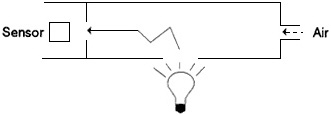
FIGURE 4-2a Approaches to the measurement of extinction. The nephelometer consists of a light-tight container that is fitted with a light source and a photodetector (represented by the sensor in the figure). The interior of the instrument is painted black and contains baffles so that the detector is not directly illuminated by the source; the detector only sees the light that is scattered from the light path. Ambient air is drawn through the instrument; the increase in the signal from the detector (compared to the signal obtained with clean, filtered air) is proportional to the scattering component of the extinction coefficient.
The nephelometer provides a point measurement, and the data obtained with it can be compared directly with other physical and chemical measurements made at the site (e.g., gas and aerosol concentration and composition and particle-size distribution). In contrast, transmissometers measure over long path lengths, at least several km (in clean air, typically 15 km), thereby yielding measurements of the mean transmittance over a long distance. Because of heterogeneities in the atmosphere, it is difficult to relate transmissometer data to chemical and physical measurements, which usually can be made only at one point or, at best, a few points.
Relationship between Particle Concentrations and Visibility
Visibility impairment is approximately proportional to the product of airborne particle concentration and viewing distance (Figure 4-3). Consequently, relatively low particle concentrations can affect visibility substantially, as shown in the following example. A dark mountain at a distance of 100 km may be clearly visible in clean air, assuming an

FIGURE 4-2b Radiance difference techniques are based on the teleradiometric measurement of adjacent bright and dark targets located several km or more from the detectors (here represented by a sensor). In transmissometry, the target radiance difference is commonly obtained by using a single, switched light source which serves as both the bright (on) and dark (off) targets. With the light off (a), the detector sees only air light; with the light on (b), the detector sees, in addition to air light, the light transmitted through the atmosphere from the source, some of which is scattered in transit. The difference in the measured radiances depends solely on the transmittance of the intervening atmosphere. (The radiances of both targets will be affected to the same degree by air light.) The average extinction coefficient (absorption and scattering combined) can be calculated if one knows the radiance difference of the targets.
average extinction coefficient of about 0.015 km-1; under such conditions, the mountain's contrast with the background sky will be about 20%. If the particle concentration increases sufficiently to increase the extinction by 0.015 km-1, the contrast will fall below the threshold for detection (about 5%) and the mountain will no longer be visible. An extinction increment of this magnitude can be produced by a relatively small concentration of fine particles, about 3–5 µg/m3 of particles with diameters between 0.1 and 1.0 µm.
Concentrations of a few µg/m3 are not unusual, even in remote regions. At these concentrations, particles usually constitute only a small
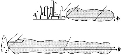
FIGURE 4-3 Visibility impairment and contaminant concentration. All other things being equal, visibility impairment depends on the product of path length and average concentration along the sight path, not on the average concentration. In this figure the two sight paths have the same total particulate mass (represented by shaded areas) along the sight path. The upper portion of the figure represents a hazy urban environment, while the lower represents a relatively clean natural setting. A photon from the target has the same chance of reaching the observer in either of the two situations; also the same number of extraneous photons (air light) will be scattered into the observer's line of sight. The radiation received by the observer is therefore the same whether the intervening atmosphere is deep and relatively clean or shallow and relatively turbid. In practice, the 'other things' of our qualifier are seldom all equal, because different extinction coefficients usually arise from differing proportions of particles and gases which could have differing scattering and absorption characteristics. Nonetheless, the simple dependence of visibility on the product of concentration and distance is a useful approximation. Among other things, it explains why the most transparent atmospheres are the most sensitive to contamination.
fraction of the total trace materials (gases and particles) found in the atmosphere, even in relatively clean regions. Sulfate (SO42), nitrate (NO3-), and organic carbon are usually the most important airborne particle fractions on a mass basis, and they are the trace materials that usually reduce visibility the most. The sulfur in 1 µg/m3 of ammonium sulfate aerosol is equivalent to 0.2 ppb of sulfur dioxide (SO2). This
SO2 gas-phase equivalent is low compared with the concentration found in a typical urban region. (The National Ambient Air Quality Standards permit 24-hour-average SO2 concentrations of up to 140 ppb. If this quantity of SO2 were converted to ammonium sulfate aerosol, the resulting concentration would be 700 µg/m3.) Indeed, the equivalent gas phase SO2 concentration calculated in this example for 1 µg/m3 of SO42is below the detection threshold of the instruments normally used to monitor compliance with SO2 air-quality standards (see Appendix B). In contrast, transmissometers easily and accurately can measure the light extinction produced by several µg/m3 of particles while nephelometers can do the same by fractions of a µg/m3 (see Appendix B). Similar conclusions hold for the gas-phase equivalents of typical nitrate and organic carbon particle concentrations.
Empirical Relationships between Airborne Particles and Visibility
The components of extinction (i.e., particle and gas scattering and absorption) and their relationship to visibility have been well characterized in a wide range of environments. These empirical relationships are shown in Figures 4-4 a-d. The relationship between visual range and the scattering coefficient (as measured with an integrating nephelometer) is shown for an urban area (Seattle) in Figure 4-4a and for an area near Shenandoah National Park in Figure 4-4b. If atmosphere and illumination are uniform, visual range and extinction in theory are inversely proportional. Because scattering is almost always the dominant component of atmospheric extinction, visual range should be inversely related to scattering as well. Figures 4-4a and 4-4b empirically confirm this expectation for hazy conditions, where sightpaths are relatively short and air masses are fairly uniformly mixed.
Figures 4-4c and 4-4d illustrate the relationship between atmospheric light extinction, as measured with nephelometers, and particle concentrations. Figure 4-4c (for Seattle) and Figure 4-4d (for an area outside of Shenandoah National Park) show that scattering is approximately proportional to total particle mass.
Figure 4-5 shows the fraction of the non-Rayleigh extinction attributable to the various components of scattering and absorption. In all

FIGURE 4-4a Empirical visibility relationships. Light scattering coefficient as a function of prevailing visibility (visual range attained over at least half of the horizon circle), in Seattle. Data are from summer 1968 at humidities below 65%. Visual range was determined by human observer; light scattering was measured by unheated nephelometer and is corrected to a photopic spectral response. Both scales are logarithmic; sloping line indicates the theoretical Koschmieder (1924) relationship V = 3.9/bext for a contrast threshold of 0.02. Source: Reprinted from Atmospheric Environment 3:543–550, H. Horvath and K.E. Noll, ''The relationship between atmospheric light scattering coefficient and visibility,'' 1969, with permission from Pergamon Press Ltd., Headington Hill Hall, Oxford, OX3 OBW, UK.
cases, fine-particle scattering is the dominant contributor to light extinction; this is especially true for eastern locations. In the West, coarse-particle scattering (usually soil dust) and particle absorption also contribute significantly.
In all regions, gases have a minor role. The only atmospheric trace gas contributing to visible extinction is nitrogen dioxide (NO2), which has a broad absorption band at the blue end of the spectrum; consequently, when NO2 concentrations are high, the atmosphere has a distinct

FIGURE 4-4b Visual range as a function of the light scattering coefficient, just outside Shenandoah National Park. Data were obtained during non-overcast conditions when the atmosphere was well mixed during mid-summer 1980. Visual range was determined by human observation of mountain peaks aligned to the southwest of the site; easily identified peaks were available at 2–3 km intervals from 5 to 24 km. Light scattering was measured by unheated nephelometer and is plotted on a reciprocal scale, in accordance with the Koschmieder (1924) relationship V ![]() 1/bext. Source: Adapted from Ferman et al., 1981.
1/bext. Source: Adapted from Ferman et al., 1981.
red-brown color. However, NO2 is relatively reactive, and its concentration is generally small, except in urban areas near emissions sources. Therefore it usually is a small contributor to regional optical air quality.
Aerosol Chemistry and Particle Size Distributions
The optical effects of atmospheric aerosols depend on the chemical composition and size distribution of the airborne particles. Particle size distributions in the atmosphere change with time; the size distribution is determined by the characteristics of the particles emitted directly by a
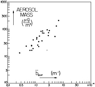
FIGURE 4-4c Particle mass concentration as a function of light scattering coefficient, in Seattle. Data are from winter 1966, averaged over periods of 2 hours to 24 hours. Light scattering was measured by unheated nephelometer, mass by a total filter located in the nephelometer outlet. Both scales are logarithmic. Source: Reprinted from Atmospheric Environment 1:469–478, R.J. Charlson, H. Horvath, and R.F. Pueschel, "The direct measurement of atmospheric light scattering coefficient for studies of visibility and pollution," 1967, with permission from Pergamon Press Ltd., Headington Hill Hall, Oxford, OX3 OBW, UK.
source, the subsequent formation of airborne particles by reactions of the emitted gases (especially SO2), and processes that remove the particles and gases from the atmosphere. Those processes are sensitive to variations in the composition of the emissions and to meteorological conditions, including sunlight intensity, temperature, humidity, and the presence of clouds, fog, or rain.
Primary airborne particles are those emitted directly from a source—for example, soot, fly ash, and soil dust, but a major portion of the fine-particle mass fraction (particles with diameters between 0.1 and 1.0 µm) usually is formed in the atmosphere by the conversion of species emitted
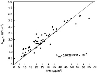
FIGURE 4-4d Light scattering coefficient as a function of fine particle mass concentration, outside Shenandoah National park. Data are 8-hour averages from midsummer 1980. Light scattering was measured by heated nephelometer and mass by a co-located filter sampler behind a cyclone separator. Source: Adapted from Ferman et al., 1981.
as gases (see Appendix A). These secondary particles include SO42, NO3-, and organic compounds. Figure 4-6 gives a qualitative overview of the processes by which secondary particles are formed in the atmosphere. The figure shows the relationships between trace gas molecules and the secondary particles that are generated from them. The generation of secondary particles begins with the generation of oxidants such as OH and O3 in the presence of sunlight and proceeds through the interaction of various reactive, transient species with various pollutant molecules (e.g., SO2, NO2, and VOCs). Heterogeneous chemistry in clouds and fog are important in many of these processes. For further discussion and a more quantitative explanation of the transformations of gases into airborne particles, see Appendix A.
The effects of primary particle emissions and chemical transformations on atmospheric particle size distributions are illustrated in Figure 4-7 (see Appendix B for particle size measurement techniques). Nucleation-mode particles (particles with diameters < 0.1 µm) can be emitted
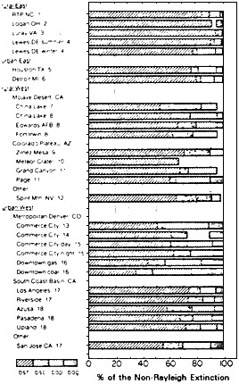
FIGURE 4-5 Additive components of extinction. This summarizes the relative contributions of components of extinction, excluding Rayleigh extinction, as determined in various field studies. The extinction attributable to each component is expressed as a fraction of the total non-Rayleigh extinction. The components are: bsf, scattering by fine (diameter < 2.5 µm) particles; bsc, scattering by coarse (diameter < 2.5 µm) particles; bap, absorption by particles; and bag, absorption by gases.
The figure clearly shows that fine particle scattering is the dominant component at all locations. The relative amounts of extinction components vary considerably showing clear regional trends. Source: Reprinted from Atmospheric Environment 24:2673–2680, W.H. White, "The components of atmospheric light extinction: A survey of ground-level budgets,' 1990, with permission from Pergamon Press Ltd., Headington Hill Hall, Oxford, OX3 OBW, UK.
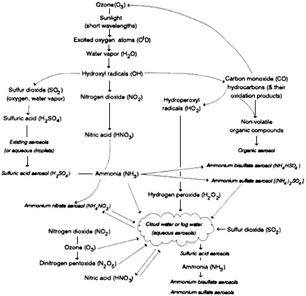
FIGURE 4-6 Pathways to secondary particle generation in the atmosphere. The diagram shows the relationships between the trace gas molecules (italicized) and the secondary that are generated from them. (See Appendix A for further discussion).
directly into the atmosphere from combustion sources or formed in the atmosphere by homogeneous nucleation. Coarse particles (particles with diameters > 1 µm) include wind-blown dust, plant particles, sea spray, and volcanic emissions. Secondary reaction products (especially NO3-) also are found on the surfaces of coarse particles (e.g., Savoie and Prospero, 1982; John et al., 1990). Accumulation mode particles (particles with diameters between 0.1 and 1.0 µm) can be primary or secondary particles; the latter are usually dominant.
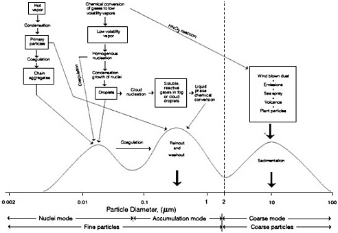
FIGURE 4-7 Trimodal size distribution. Schematic diagram of an airborne particle surface area distribution showing the three modes, the main source of mass for each mode, the principal processes involved in inserting mass into each mode, and the principal removal mechanisms for the modes. Source: Adapted from NRC, 1981.
The physics and chemistry of atmospheric particle formation results in a trimodal size distribution. Those size differences have a profound effect on the physical and optical properties of the resulting aerosol. The characterization of aerosol effects is further complicated by the highly dynamic nature of particle size distributions. Particle size is affected not only by a wide range of formation and transformation processes but also by atmospheric removal processes. Particles are removed from the atmosphere by wet processes (precipitation, cloud, and fog) and dry processes (gravitation, diffusion, and impaction).
Large particles settle toward the earth, with sedimentation velocities proportional to dp2 (Friedlander, 1977). Loss rates are proportional to sedimentation velocities, and therefore the rates increase rapidly with increasing particle size. In contrast, small particles are highly mobile and are lost primarily through attachment to other particles that they encounter during their random motions. The resulting loss rates for the smallest particles are proportional to their diffusion coefficients, yielding a dependence on particle size in the range dp-2 to dp-1 (Friedlander, 1977). Other diffusional losses (e.g., within control devices or to vegetation) display a similar dependence on particle size.
The efficiency of wet removal processes is also highly size-dependent (see the section below, The Role of Meteorology). The net result of the various wet and dry removal processes is that particles in the nucleation and coarse-modes tend to have a relatively short residence time while those in the accumulation mode have a relatively long residence times (see Figure 4-8). In the next section, we show that these long-lived accumulation-mode particles have the greatest effect per unit mass on visibility and that it is for this reason that visibility impacts can often extend over large regions.
Particle Optics and Visibility
The optical properties of airborne particles are affected by several factors, among them particle size. Figure 4-9 shows the scattering efficiency of ammonium sulfate particles as a function of their diameter for monochromatic 530 nm light. The oscillations that are shown correspond to size-dependent resonances in scattering. For white light, a smooth curve that peaks at about the same particle size is found. The
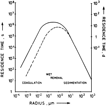
FIGURE 4-8 Particle loss rates as functions of particle size. Particle loss mechanisms are dependent on particle diameter. By comparing this figure with Figure 4-9, which shows particle scattering efficiency as a function of particle size, one sees that none of the common removal mechanisms is very effective in removing particles that are the most efficient scatterers of light. This fact accounts for the accumulation and persistence of large hazy air masses. Source: Jaenicke, 1980.
size-dependent scattering efficiencies of other types of airborne particles are qualitatively similar. A given mass concentration scatters most effectively when it is distributed among particles having diameters comparable to the wavelength of the illumination (Friedlander, 1977).

FIGURE 4-9 Dependence of light scattering on particle size. The scattering efficiency of particles depends on several factors, among them particle size, wavelength of the light, and optical properties of the aerosol material. The theoretical scattering efficiency can be computed as shown here for ammonium sulfate particles at wavelength 530 nm (the curve labeled (NH4)2 SO4). Particles scatter light most effectively when their diameters are comparable to the wavelength of the illumination (Friedlander, 1977). Therefore, airborne particles, which tend to accumulate in the size range 0.1 to 1.0 µm diameter, can have a large effect on visibility. Particles much larger than the wavelength of visible light show a sharply decreasing scattering efficiency with increasing particle size. These particles scatter energy in proportion to their geometric cross-sectional area; that is, they "cast shadows" just as larger objects do. However, for particles (and gas molecules) much smaller than the wavelength of visible light, the scattering efficiency increases rapidly with increasing particle (and gas molecule) size (a few tenths of a µm or less); these particles scatter energy in proportion to the square of their mass. In the size range of about 0.3–1.0 µm, the scattering behavior of particles is very complex. Source: Adapted from Ouimette and Flagan, 1982.
Secondary particles can have a strong effect on visibility and visibility impairment because these particles tend to accumulate in the size range of 0.4–0.7 µm, the region of the range for the visible spectrum.
Figure 4-10a shows the production rates of excess aerosol sulfur (i.e., the SO42- aerosol concentration in excess of that in the regional background aerosol) as a function of solar age of the St. Louis urban plume. The solar age is the equivalent number of hours of exposure to clear-sky midday solar radiation. The data show that secondary sulfur particle production varies roughly linearly with solar age. The data are consistent with the conversion of SO2 to SO42- at average rates that range from 2% to 4% per hour. Figure 4-10b shows (for the same data set) the change of the excess aerosol light-scattering cross section as a function of solar age. It is important to note that nearly all the light scattering is due to secondary particles and that the emissions from sources in St. Louis have their greatest effects a considerable distance downwind.
Figures 4-7, 4-8, and 4-9 illustrate the relationship between the visibility problem and pollution:
-
Sources emit gases that are converted to secondary airborne particles,
-
Those particles are produced primarily in the 0.1–1.0 µm diameter range,
-
The 0.1–1.0 µm size range is where the light scattering per unit mass is greatest and where removal rates are slowest.
Because the secondary aerosol particles have long lifetimes, they can be carried great distances by winds; consequently, visibility impairment is usually a regional problem. Further, these particles are small, and they have a large effect on visibility per unit mass. It follows that visibility impairment is a sensitive indicator of air pollution, and visibility can be significantly improved only by addressing the problem on a regional scale.
Some Experimental Difficulties in Aerosol Chemistry Studies
Because of the relationship of visibility to various airborne particles
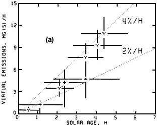
FIGURE 4-10 a, b Increase in light-scattering aerosol with distance from source. This figure show measured flow rates of excess (a) sulfate particles (Mg sulfur/hour) and (b) light scattering coefficient (km 2/hour) downwind of metropolitan St. Louis. The data were obtained from a detailed mapping of the urban plume by instrumented aircraft, together with intensive pilot balloon determinations of wind. Observations are plotted as a function of 'solar age', in equivalents of exposure to clear-sky midday solar radiation. These data show that most of the sulfate and light-scattering aerosol attributable to St. Louis is formed in the atmosphere hours downwind of the city; the sulfate is generated by the photochemical oxidation of SO2 that is emitted from sources in St. Louis and carried away by the winds. Dotted lines in (a) indicate sulfate flow rates that would be expected for SO2 conversion rates of 2% and 4% per hour. Source: White et al., 1983.
and their size distributions, it is important that aerosol composition and particle-size distributions be measured accurately in visibility programs. In practice, such measurements are difficult. (A more detailed discussion is found in Appendix B.)
One problem is that most of the important gas and particulate phase species are highly reactive. Of particular concern is the conversion of gas-phase species within a sampling system; gas concentrations can be hundreds of times greater than those of the ambient airborne particle

equivalents. For example, glass fiber filters were used for many years to collect particulate matter. In the late 1970s, it was found that these chemically basic glass fibers efficiently captured gaseous nitric acid, and yielded erroneously high values for particulate NO3-. As discussed in Appendix B, there are many other cases where gas-phase species react with the sampling medium to yield erroneously high particle concentrations.
The reverse process can occur as well. Aerosol substances can react in a sampling system to produce gaseous materials that are lost to the sampling stream. For example, Teflon filters, which are chemically inert, yield erroneously low NO3- aerosol values because of nitrate volatilization. When ambient NO3- particles (which must have been neutral or basic to exist in the atmosphere) are collected on the filter surface, they can react with acidic SO42- particles or with SO2 in the air stream; as a result, NO3- is converted to nitric acid, which subsequently evaporates.
One solution to these problems is to strip the gas-phase species such as nitric acid from the air stream before passing it though the filter. This is accomplished by a combination of gas denuders and filter packs (Figure 4-11). These sampling systems yield reliable measurements of
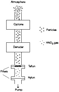
FIGURE 4-11 Phase-preserving particle sampling train. A combination of denuders and filter packs can be used to obtain a sample of particles and gases that is representative of the ambient atmosphere, because it minimizes interaction between various reactive species. The sample is drawn through an inertial separator (a cyclone) to remove large particles (> 2.5 µm diam.) that would be subject to losses in the denuder. The air stream is then drawn through a denuder to remove gaseous nitric acid, which might form artifact particulate nitrate through reaction on the filter. The denuder typically consists of parallel plates or concentric cylinders separated by a few mm and coated with a reagent; the path length through the denuder is typically a few tens of cm. The denuder exploits the fact that gases are much more diffusive than particulate phases. After passing through the denuder, the air stream is drawn through a filter pack. The pack consists of a Teflon filter to collect particles, followed by a reactive filter (usually nylon) that will capture any nitric acid released from the particles collected on the Teflon filter. The sum of the nitrate collected in the cyclone and on the front and backup filters yields the total concentration in the particulate phase. The nitrate in the denuder is assumed to be derived from the gas-phase nitric acid. Additional denuder stages can be added in series to collect other gaseous substances (e.g., SO2, NH3 etc.) according to the reagent coating employed in the denuder. For additional information, see Appel et al. (1981); Forrest et al. (1982); Shaw et al. (1982); Eatough et al. (1988); Wiebe et al. (1990).
ambient fine-particle NO3- concentrations and of the gaseous nitric acid. With the addition of various denuders in series (or with two or more denuder/filter pack systems in parallel) these systems can be used to collect other gas-phase species (e.g., SO2, NH3, and HCl).
Water presents another problem. Because most of the aerosol particulate mass consists of hygroscopic materials (e.g., sulfuric acid, ammonium sulfate, ammonium bisulfate, and ammonium nitrate), the size of the airborne particles depends on the relative humidity. For a change in relative humidity from 30% to 90%, the size of an ammonium sulfate particle increases by a factor of 5, while a sulfuric acid particle grows by a factor of more than 3 (Figure 4-12). The air in the lower atmosphere usually contains a substantial amount of water (typically several g/m3) even in the arid Southwest. Because the concentration of water vapor is millions of times greater than that of airborne particles, the conversion (condensation, sorption, or reaction) of even a minute fraction of this water to the particulate phase can have a major effect on visibility. Hygroscopic particles can take up water at humidities well below saturation. It follows that particle-borne water can play a major role in optical extinction at high relative humidities (> 70%) (see Figure 4-13).
Even though water itself is a natural constituent of the atmosphere, in the context of visibility impairment, the water associated with anthropogenic SO42- and NO3- must be regarded as a contaminant since it condenses to further degrade visibility in the presence of hygroscopic particles. The direct measurement of particulate water is a formidable challenge. Because the water associated with particles constitutes only a small fraction of the total water, it cannot be collected using denuders and filter packs. As discussed further in Appendix B, techniques are needed to quantify particle water content.
THE ROLE OF METEOROLOGY
Meteorology can play a dominant role in visibility degradation. For example, wind speed either can reduce or increase the likelihood of visibility degradation. At low wind speeds, the ventilation of emitted pollutants is reduced, thus increasing the concentration of pollutants in the atmospheric boundary layer. High winds can also degrade visibility
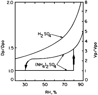
FIGURE 4-12 Dependence of particle size on composition and relative humidity. Under many common ambient conditions, much scattering associated with hygroscopic particles could be attributable to water held in the liquid phase. The interaction with water vapor can be complex and vary strongly with chemical composition. This figure shows the difference between behavior of H2SO4 and (NH4)2SO4 particles, two common pollutant aerosol species. H 2SO4 drop-lets pick up (and lose) water readily over a wide range of RH values. (NH 4)2SO4 has much more complex behavior. When an (NH4)2SO4 particle is exposed to increasingly moist air, it does not pick up water vapor until RH reaches 79.5 %, the deliquescence point for the salt; at this point, the droplet grows rapidly (indicated by the upward-pointing ar-row). When droplets of (NH 4)2SO4 solution are exposed to increasingly dry air, the salt retains water to RH well below the deliquescence point, and the solution becomes supersaturated. Clearly, it is not enough to know the concentration of sulfate in the atmosphere; speciation must be known, because the difference in the behavior of H2SO4 and (NH4)2SO4 particles is large, especially at low RH values. Also, note that the deliquescence point is at an RH value that is common in many regions, especially during the summer. Source: Adapted from Tang, 1980.
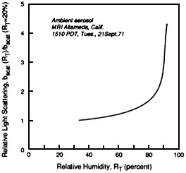
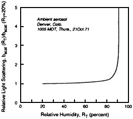
FIGURE 4-13 Atmospheric measurements of light scattering as a function of relative humidity. The observed dependence of particle light scattering on relative humidity (RH) at two locations, Altadena, CA, and Denver, as measured with an integrating nephelometer. The relative humidity of the air stream entering the nephelometer is varied from 20% to over 90% and the change in scattering is recorded. The figure presents the results as the ratio of the scatter measured at a specific RH to that measured at 20% RH. At Altadena the scatter increased continuously over the entire range of RH (especially above 80%) in a manner similar to that for H2SO4 in Figure 4-12. Light scatter increases about a factor of two between 20% and 85% RH. This suggests that the Altadena particles are very hygroscopic and that visibility effect vary greatly with RH. In contrast, Denver particles are relatively are very hygroscopic; there is very little increase inscatter until the RH exceeds 90%. These data demonstrate that scattering is very sensitive to RH and that the behavior of airborne particles with respect to RH can differ with location, depending on the composition of the particles. Source: Covert et al., 1972.
locally by picking up and carrying dry soil. When low wind speeds are associated with low temperatures (as is common in the western United States during winter), stagnation occurs and pollutants accumulate. Pollutants may build up further during periods of low temperature due to increased heating requirements (e.g., increased power-plant emissions and wood smoke).
The following section discusses some examples of the role of meteorology in visibility. Appendix A discusses meteorological factors in more detail.
Transport
The transport of atmospheric pollutants depends strongly on meteorological conditions. For example, high SO42- concentrations in the Adirondack Mountains most often are associated with transport from polluted regions to the south and southwest of New York (Galvin et al., 1978). In the Shenandoah Valley, 78–86% of the light extinction is attributed to anthropogenic airborne particles, most of which originate in the Midwest (Ferman et al., 1981).
Presently there is good understanding of the meteorological factors that affect regional haze transport in the eastern United States. However, knowledge about meteorological effects on visibility in the West is less advanced. It is known that in the western and northwestern United States, the types of meteorological conditions associated with decreased visibility change seasonally. Incidents of reduced wintertime visibility in the Southwest usually are associated with low wind speeds and high relative humidities (NPS, 1989). In pristine regions, where the visual range can be great, small increases in SO42- aerosol concentrations can lead to readily apparent decreases in visibility. Consequently, visibility in those areas is sensitive to meteorological conditions that maximize the effect of local emissions or transport emissions from distant sources.
In the Southwest, the winter episodes of decreased visibility usually occur during mesoscale meteorological events. Few data are available with which to delineate the areal coverage of these haze episodes. Nonetheless, evidence from the WHITEX study suggests that the spatial extent of haze during that study was small compared with the size of haze episodes in the East. Southwestern episodes are, however, too
large to be accommodated by the predictive techniques used for plume blight; plume models typically are restricted to sources within 50 km of the receptor. Thus, adequate plume models are not available for dealing with the western haze episodes.
During the summer in the Southwest, decreased visibility is associated with a wide range of meteorological conditions. Winds can carry heavily polluted air from southern California eastward to regions of the desert Southwest, including the Grand Canyon National Park. Similar conditions occur in the San Joaquin Valley, where winds carry pollutants from the San Francisco Bay area toward the national parks of the Sierra Nevadas.
Meteorology also plays an important role in the chemical transformation of pollutant gases to particles. Conversion of SO2 to SO42- is greatly accelerated in the presence of water droplets, in particular fog or cloud droplets (see Appendix A). Figure 4-14 shows the ratio of particulate sulfur (i.e., SO42-) to total sulfur (primarily SO2 and SO42-) as a function of plume age. The figure summarizes data obtained in measurements from a variety of sources by many different investigators. Figure 4-14 shows that from < 1% to > 10% of the SO2 can be converted to light-scattering SO42- aerosol particles after several hours. Thus, the effect of a particular source on a receptor region can vary tremendously, depending on ambient atmospheric conditions.
It is clear that the meteorological conditions associated with reduced visibility in national parks and wilderness areas in the West are different from those in the East. Consequently, a range of meteorological analysis options needs to be devised to attribute haze to sources in the two areas.
Dispersion
The stability of the atmosphere affects the amount of vertical mixing that takes place during plume transport. Enhanced mixing reduces pollutant concentrations near the sources (i.e., within a few tens of kilometers). The transport path of a plume is determined by the wind speed and direction combined with the effects of vertical mixing. Strong vertical mixing dilutes the plumes, making them less dense and less visible.
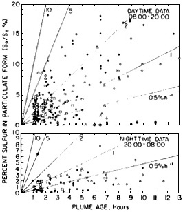
FIGURE 4-14 Extent of gas-to-particle sulfur conversion as a function of emissions age for daytime (top) and nighttime (bottom). Sp/St is the ratio of particulate sulfur (mostly SO 42-) to total sulfur (mostly SO42- and SO2). The data are collated from measurements made in the plumes of 12 different point sources, as reported by 8 different organizations. The concentrations S p and St have been corrected for background and primary particle contributions. Different symbols distinguish the data from different reporting organizations. Data corresponding to plume ages of less than I hour are not shown. The lines are labeled for different nominal conversion rates (%/hour). Note that daytime rates are considerably greater than nighttime rates. Source: Reprinted from Atmospheric Environment 15:2573–2581, W.E. Wilson, Jr., ''Sulfate formation in point source plumes: A review of recent field studies,'' 1981, with permission from Pergamon Press Ltd., Headington Hill Hall, Oxford, OX3 OBW, UK.
Vertical mixing also can break up surface layers into which plumes can become entrained. Vertical mixing subsequently redistributes the pollutants into a thicker layer of more homogeneous haze. In contrast, reduced mixing combined with low wind speeds can increase the likelihood of formation of valley fogs; valley fogs are often an important factor in pollution episodes, because many industrial sources are located in valleys, near water resources.
Deposition and Resuspension
The transport of particles to and from the Earth's surface has an important effect on haze. Wet and dry deposition processes cleanse the air, while the resuspension of soil dust and plant material by winds can be a significant source of visibility-impairing particles. In this section we briefly describe the role of these surface-exchange processes in visibility.
Wet Deposition
Wet deposition is the result of processes that occur within and below clouds. Field studies have shown that within clouds most (>90%) of the visibility-impairing particles are incorporated into cloud droplets (Brink et al., 1987) along with a large fraction of the reactive gases. Cloud droplets have two fates: they can be removed as precipitation or they can evaporate. It has been estimated that only about 10% of the cloud cover dissipates through precipitation; the other 90% evaporates (McDonald, 1958). When clouds evaporate, the particles that were incorporated into cloud droplets are re-released to the atmosphere. However, the composition of the resulting aerosol changes because of the aqueous-phase chemistry that takes place in cloud droplets, principally because of reactions with atmospheric gases such as SO2 and HNO3. Airborne particles are likely to cycle through clouds many times before they are removed by precipitation, and the composition and size of the particles changes with each cycle. This process accounts for the fact that individual particles are often found to consist of internal mixtures of a wide range of chemical species (Andreae et al., 1986)
It is generally believed that, because of the very large surface-to-volume ratio of cloud droplets, in-cloud processes are more effective than the below-cloud processes at cleansing the atmosphere of visibility-impairing particles and their gaseous precursors. Particles and gases also can be removed below cloud level by falling precipitation; however, the mass transfer to precipitation is relatively inefficient due to the large droplet sizes.
Dry Deposition
Dry deposition is the deposition of particles and gases to surfaces in the absence of precipitation. Dry removal rates of particles from the atmosphere depend on particle size, small-scale meteorological processes near the surface, and the chemical and physical characteristics of the receiving surface. Studies suggest that dry deposition typically accounts for roughly 20% to 40% of the sulfur removal from an airshed (Shannon, 1981). Young et al. (1988) estimated that dry deposition contributes about half of the acid deposition in mountainous regions of the western United States, although it might be less important than wet deposition in the eastern United States (Galloway et al., 1984). Dry deposition has been reviewed by McMahon and Denison (1979), Sehmel (1980), Hosker and Lindberg (1982), and Davidson and Wu (1989).
Theory shows that dry deposition rates of particles are lowest for particles in the 0.05–0.5 µm diameter range. Therefore, particles in this size range have a longer atmospheric lifetime than smaller or larger particles. This is significant from the standpoint of haze formation, because particles of this size are relatively effective at light scattering and absorption.
Resuspension of Soil Dust
The resuspension of soil dust is an important source of coarse atmospheric particles. Although those particles have relatively short atmospheric lifetimes, they can reduce visibility considerably under some conditions. Soil dust is resuspended by dust devils, wind erosion, agricultural tilling, and vehicular travel on paved and unpaved roads. Gillette and Sinclair (1990) found that resuspension of soil dust by dust devils is comparable in significance to other sources of that material. Vehicular travel is an important anthropogenic source. All estimates show that emissions of soil dust are higher in the arid Southwest than in other parts of the United States.
STRATEGIES FOR VISIBILITY MEASUREMENT PROGRAMS
The preceding sections discussed visibility measurement techniques
without regard for the manner in which they might be integrated into a visibility study. In practice, such studies are performed in either a research or an operational mode:
In a research (or intensive) mode, a large array of measurements is made to understand the factors affecting visibility. Intensive studies often involve a large cooperative effort by scientists from academic, government, and private organizations. Such studies normally take place over a short period—weeks to a few months.
In a monitoring mode, measurements are made routinely over an extended period—usually many years—to detect and characterize patterns in visibility impairment and to identify the causes of such patterns. Standardized instrumentation is used in such studies and the procedures must be simple enough to be carried out by personnel without highly specialized training.
This section focuses on systems and procedures used in field measurement programs and different strategies for establishing a visibility monitoring program.
Criteria for Monitoring Programs
In monitoring programs, the optical properties measured are those that are closely related to human visual perception. Regulatory agencies with monitoring responsibilities design optical measurement programs on the basis of several practical considerations:
-
The measurement methods should be inexpensive, reliable, and simple to operate under field conditions. Because extinction coefficients are likely to vary widely for monitoring programs that cover a wide geographical area, these methods should be capable of measuring the extinction coefficient over several orders of magnitude.
-
The extinction data should be coordinated with measurements of the concentrations of atmospheric aerosols that cause the extinction so that source-apportionment analysis based on aerosol chemistry can be linked to extinction.
-
The measurements should reflect visibility conditions as perceived by human observers, and the measured parameters should be presented in units that are understandable to decision makers and the public.
-
Because the Clean Air Act and regulatory programs focus on anthropogenic rather than natural sources of visibility impairment, the
-
method should be insensitive to extinction caused by rain, fog, snow, and other weather conditions.
-
Data-averaging times should be linked to the public perception of visibility (e.g., a 24-hour averaging period is of little or no help when regulators are concerned with visibility impairment only during the daylight hours).
These criteria can be difficult to meet. Visibility as perceived by a human observer cannot be fully replicated by any instrumental technique (see Appendix B). Because no single method can satisfy all of these criteria, regulatory agencies (which usually have very limited funding) must often rank their monitoring needs.
Monitoring meteorological variables in support of an assessment of regional haze should be conducted with these considerations in mind:
-
At a minimum, the field program should be based on an analysis of the climatology of low-visibility episodes. The analysis should involve data on the wind flow, humidity, and atmospheric stability conditions most often associated with low-visibility episodes.
-
Meteorological instruments should be sited to represent the air flow at suspected or proposed sources or source areas, at key receptor areas, and at intermediate locations. Wind measurements should represent the wind flow at the height of the emission plume, which usually requires aloft measurements of winds aloft.
Examples of Visibility Measurement Programs
The Interagency Monitoring of Protected Visual Environments Program
In response to Section 169A of the 1977 Clean Air Act Amendments, EPA promulgated regulations for a visibility monitoring strategy for Class I areas for states that have not incorporated such strategies in their state implementation plans (SIPs). The federal strategy called for the establishment of an interagency program with the cooperation of EPA and several federal land management agencies, including the National Park Service (NPS), the Fish and Wildlife Service (FWS) and the Bu-
reau of Land Management (BLM) of the U.S. Department of Interior, and the Forest Service (FS) of the U.S. Department of Agriculture. The Interagency Monitoring of Protected Visual Environments (IMPROVE) program has been operating since March 1988 to satisfy the regulatory requirements.
The objectives of IMPROVE are (1) to characterize background visibility so as to be able to assess the effects of potential new sources, (2) to determine the present sources of visibility impairment and to assess the amounts of impairment from these sources, (3) to collect data that are useful for assessing progress toward the national visibility goal, and (4) to promote the development of improved visibility monitoring technology and the collection of visibility data (Pitchford and Joseph, 1990).
Twenty sites now operate in the IMPROVE network. Additional sites that employ similar measurement methodologies are operated by NPS in the TERPA (Tahoe Regional Planning Agency) and NESCAUM (Northeast States for Coordinated Air Use Management) networks. Figure 4-15 gives the locations of the 48 sites using the IMPROVE sampler. These networks are operated by Cahill and co-workers at the University of California at Davis.
The IMPROVE measurement protocol involves aerosol, optical, and view monitoring. Four particle samples are collected simultaneously over 24 hours on Wednesdays and Saturdays each week. The samplers include one PM10 filter sampling system (which collects particles smaller than 10 µm diameter) and three PM2.5 filter systems (for particles smaller than 2.5 µm). One of the PM2.5 samplers is preceded by a potassium carbonate denuder to remove acidic gases so as to facilitate the measurement of particulate nitrates. Table 4-1 indicates the measured quantities and the analytical techniques used for each filter type. All of the filter analyses are done at the University of California at Davis, except for ion chromatography (IC) and thermal optical reflectance (TOR), which are subcontracted to other laboratories (Pitchford and Joseph, 1990). Temperature and relative humidity measurements are made with rotronic model MP-1007 humidity temperature meteorological probes. According to manufacturer's specifications, these sensors record RH to "within a few %RH over the temperature operating range of the probe." The operating temperature range is-20°C to + 55°C.
The IMPROVE sampling strategy provides information on major and trace particulate species. The TOR measurements of organic and ele-
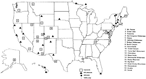
TABLE 4-1 Particle Measurements Made with the Interagency Monitoring of Protected Visual Environments (IMPROVE) Samplera
|
|
Filter Type |
Quantity Measured |
Analytical Technique |
|
Module A |
Fine teflon filterb |
Mass of collected particles |
Gravimetric analysis |
|
|
|
Optical absorption (babs) |
Laser integrating plate method |
|
|
|
Elements Na to Pb |
Particle-induced X-ray emission |
|
|
|
Hydrogen |
Proton elastic scattering |
|
Module B |
Sodium carbonate denuder and fine nylon filterb |
Chloride, nitrite, nitrate, sulfate |
Ion chromatography |
|
Module C |
Fine quartz filterb |
Organic and elemental carbon |
Thermal optical reflectance |
|
Module D |
PM10 filterb |
Mass of collected particles |
Gravimetric analysis |
|
|
Impregnated quartz filterc |
SO2 |
Ion chromatography |
|
a The IMPROVE Modular Aerosol Monitoring Sampler consists of four independent filter modules, a control module, and a pump house containing a pump for each module. Each module collects two 24-hour filter samples per week. The filters are collected weekly and shipped to laboratories for analysis. b The three fine filters collect particles of diameter less than 2.5 µm. The PM10 filter collects particles of diameter less than 10 µm. c This filter, which collects gaseous SO2, is used in samplers at National Park Service Criteria Pollutant Monitoring sites. Samplers at these sites are otherwise identical to samplers at IMPROVE sites. Sources: Eldred, 1988; Pitchford and Joseph, 1990; R. Eldred, pers. comm., University of California at Davis, July, 1992. |
|||
mental carbon particulate concentrations are likely to be the least accurate measurements. An independent estimate of particulate carbon concentrations is obtained from proton elastic scattering analysis (PESA) measurements of hydrogen (e.g., Eldred et al., 1989) using the nonsulfate hydrogen technique. In this procedure, the amount of hydrogen associated with SO42- is subtracted out by assuming that the SO42- consist of pure ammonium sulfate; for samples collected at Great Smoky Mountains and Shenandoah, the SO42- is assumed to be 75% ammonium sulfate and 25% sulfuric acid (e.g., Eldred et al., 1989). It is further assumed that hydrogen associated with nitrates or water is lost when the sample is brought to vacuum during PESA analysis. The resulting hydrogen concentration is converted to an equivalent carbon value by assuming that hydrogen constitutes 9% of the organic mass. These assumptions yield surprisingly good correlations between TOR and PESA estimates of carbon concentrations. It would be far preferable, however, to measure particulate carbon more accurately and directly, for reasons to be discussed below.
Transmissometers are used to measure extinction coefficients in the IMPROVE network. Temperature and relative humidity are also measured continuously on site. Data from these instruments are radio-transmitted via satellite to a central computer for daily retrieval; thus, malfunctions can be discovered quickly and remedied.
There is a major concern about the quality of the data obtained in the IMPROVE network. Because of limited resources, comprehensive quality assurance evaluations have not been carried out by independent auditors. However, intercomparisons with various measurements from other groups have been done in conjunction with several intensive field programs. Also, outlier points can be identified through comparisons among interrelated variables (Pitchford and Joseph, 1990). Nonetheless, it is essential that the quality of these data be characterized and clearly documented so that long-term trends can be evaluated.
One example is the concern about the quality of the organic carbon concentration data estimated by the nonsulfate hydrogen technique. Data for average concentrations across the United States from June 1984 to June 1986 are approximately a factor of two lower than average concentrations measured between March 1988 and February 1989 (Cahill et al., 1989; Eldred et al., 1990). The data during the earlier period were collected with the sequential filter unit (SFU), a predecessor to the IM-
PROVE sampler that was used in the more recent measurements. It is not known whether the differences are due to an actual change in ambient concentrations (which would be surprisingly large for so short a time), to differences in the sampler operating characteristics, or to some other factor. It is essential that the reasons for such discrepancies be documented clearly.
State Programs
In this section we present some examples of state visibility monitoring programs. This discussion is not intended to be a comprehensive survey. In presenting these examples, the committee does not endorse or condemn either the design strategy for the cited programs or the manner in which they are implemented. The following examples show some approaches to state monitoring needs.
Sequential filter samplers are used for aerosol monitoring by Oregon and Washington at remote sites near Northwest Class I areas (Core, 1985). The sequential filter sampler first was developed during the Portland Aerosol Characterization Study (PACS) (Watson, 1979) and later adapted for use in the Sulfate Regional Experiment (SURE) (Mueller and Hidy, 1983). The current design (with a PM10 inlet) has been designated by EPA as an equivalent method for PM10 monitoring in Oregon.
In this system, 12-hour sampling periods provide adequate analytical sensitivities. Timers control the sampling time and intervals. As many as 12 filter sets can be loaded into the sampler at any one time, thereby minimizing the number of site visits needed to maintain continuous operation. The filters are contained in cassettes to minimize possibilities of contamination and are routinely analyzed for gravimetric mass. Selected samples are analyzed by x-ray fluorescence (XRF), IC, and TOR to provide aerosol composition data for receptor modeling and extinction budget analysis.
The state regulatory agencies of Washington, Oregon, and California measure extinction as part of their visibility monitoring programs. In each case, the states have chosen measurement methods simpler and less costly than those that would normally be used in field research programs.
The California Air Resources Board (CARB) reviewed several optical methods for measuring visibility impairment throughout the state (CARB, 1989). These included measurements of transmittance using active and passive transmissometers, of extinction caused by light scattering based on scanning and integrating nephelometers, and of light absorption as measured by the integrating plate and coefficient of haze (COH) methods. Indirect methods of measuring extinction, including contrast ratio measurements from densitometer analysis of 35-mm color slides and teleradiometry, also were evaluated, as was modeling of extinction from aerosol chemistry measurements.
Following an extensive consideration of the costs, the relative advantages and disadvantages, and the ease of implementation of the various methods, the CARB Committee on Visibility adopted three measurement methods: 1) integrating nephelometry (MRI 1550 B with heated inlet) for measuring dry particle light scattering at a nominal wavelength of 550 nm; 2) COH tape sampler measurements as an indicator of light absorption in urban areas; and 3) ambient air hygrometer measurements of relative humidity. The humidity measurements are used to flag observation periods when relative humidity exceeds 70%.
In developing monitoring protocols, California took a pragmatic point of view, opting for simple, reliable measurements of parameters that could be related to anthropogenic sources of impairment and thereby support regulatory programs. Automated cameras and densitometric radiometry were recommended as an alternative approach to document scene quality at specific levels of measured extinction.
The Oregon State Department of Environmental Quality also chose to use MRI 1550 B integrating nephelometers equipped with heated inlets as their primary measure of extinction. Important considerations in making this selection were that the method is insensitive to extinction caused by weather conditions and that the instrument is reliable. Unlike California's program, all of Oregon's monitoring is conducted at remote sites near Class I areas where absorption is a minor component (typically 8%) of the total extinction (Beck and Associates, 1986). As a result, the Oregon program does not include routine measurements of light absorption. The state's visibility goals are expressed in terms of reductions in the frequency of impairment (defined in the SIP) as measured by integrating nephelometry.
In areas where commercial power is not available, 35-mm cameras
are used to document scene quality three times daily. Standard visual range measurements are then made from the slides by densitometric radiometry.
The Washington State Department of Ecology carries out a visibility monitoring program similar to Oregon's, except that MRI 1590 integrating nephelometers (with unheated inlets) are used (principally because the equipment was available in this configuration). Like Oregon, Washington has adopted a working definition of visibility impairment (as measured by nephelometry) of 40 Mm-1, exclusive of Rayleigh scattering (State of Washington, Department of Ecology, 1983).
Washington also uses automated 35-mm cameras to document scene quality. Visual range is estimated from the slides by densitometric radiometry.
As a result of these measurement programs, Oregon and Washington have adopted restrictions on sources that impair visibility in their Class I areas.
Intensive Programs
This section describes an intensive experiment designed to evaluate the visibility effects of a particular point source, the Navajo Generating Station (NGS). In providing this example, the committee does not imply that it endorses or condemns either the design strategy or the manner in which the program was implemented.
NGS is a coal-fired power station; with a generating capacity of 2400 MW, it is one of the largest power plants in the western United States. NGS is located approximately 25 km from the nearest border of the Grand Canyon National Park and about 110 km from the Grand Canyon Village tourist area. This region experiences extended periods of stagnation during the winter; hazes are known to occur at such times. The NGS visibility study was carried out in 1990 to determine the extent to which wintertime visibility at the GCNP would be improved if NGS emissions of SO2 were reduced. (For a more complete discussion of this study, see Richards et al., 1991).
Field measurements were made in an array of sampling sites in the vicinity of NGS over an 81-day period from January to March 1990; these included air quality and optical parameters and meteorological
data. As one component of the program, the investigators injected perfluorocarbon tracers into the NGS stacks; at the monitoring sites, the concentration of this tracer was measured along with the other parameters. Various aspects of NGS emissions (concentrations of SO 2, NOx, and particles, along with opacity) also were monitored continuously during the project. Instrumented aircraft were used to characterize the composition of the NGS plume and of the regional background during selected intensive operation periods. Several special experiments were conducted to characterize the aerosol in more detail than was possible with the routine filter data.
A summary of the meteorological measurements made during the NGS visibility study is given in Table 4-2; site locations are shown in Figure 4-16. These measurements were designed to provide data for forecasting intensive operation periods and to support diagnostic modeling analyses. Surface meteorology measurements included wind direction and speed, temperature, relative humidity, precipitation, and radiation. In addition, rawinsondes, airsondes, and tethersondes were used periodically at several sites to measure winds, pressure, temperature, and relative humidity as functions of altitude. Wind fields were mapped using radar profilers, Doppler sodar, monostatic sodar, and Doppler lidar.
Surface air quality measurements were made at 27 sites. Table 4-3 summarizes the measurements made at these sites; the locations of tracer and air-quality monitoring sites are shown in Figure 4-17. Not all of the measurements listed in Table 4-3 were made at all sites. However, certain measurements, such as SO2 and SO42- concentrations and fine particle mass were made routinely at most sites. Other measurements, such as organic and elemental carbon concentrations, size-resolved aerosol chemical composition, aerosol water content, cloud water chemistry, and aerosol optical measurements, were made at selected sites. Approximately 60,000 substrates were analyzed for particulate mass and chemical composition.
Two approaches were used to determine the effect of NGS emissions on haze. One approach was largely empirical: the data were examined to determine the relationships among NGS emissions, meteorology, air quality, and visibility during the study period. The second approach involved mechanistic modeling. The contributions of NGS and other sources to SO42- levels in the study area were obtained by numerical

FIGURE 4-16 The locations of meteorological measurement sites in the experimental area for the 1990 NGS Visibility Study. Source: Richards et al., 1991.
The field program was designed so that measurements provided the required information for each analytical approach.
An intensive study of this kind can provide detailed information on factors that affect visibility. One major limitation of intensive programs is that they are confined to relatively short periods. Because year-to-
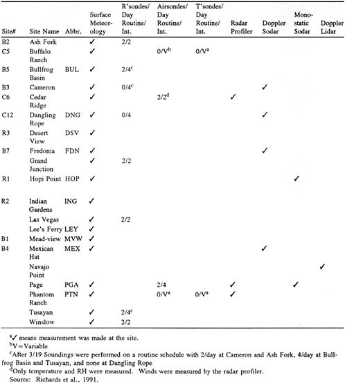
TABLE 4–3 Measurement Methods
|
Parameter |
Sampling Methoda |
Sampling Frequency |
Durationb |
|
PM2.5: |
|
|
|
|
Mass |
Filter sampling |
6/day |
4 hours |
|
|
|
3/day |
8 hours |
|
|
|
2/day |
12 hours |
|
Sulfate (total sulfur) |
Filter sampling |
6/day |
4 hours |
|
Nitrate |
Filter sampling |
3/day |
8 hours |
|
Carbon |
Filter sampling |
3/day |
8 hours |
|
Trace elements |
Filter sampling |
3/day |
8 hours |
|
Size fractionated |
DRUM |
3/day |
8 hours resolution |
|
Trace elements |
|
|
|
|
Size fractionated |
MOUDI |
Daily |
24 hours |
|
Multiple species |
|
|
|
|
Water |
TDMA |
Continuous |
— |
|
Sized fractionated |
LPI |
3/day |
8 hours |
|
Sulfate |
|
|
|
|
Gases: |
|
|
|
|
SO2 |
Filter pack |
6/day |
4 hours |
|
NO/Nox, SO2, O3 |
Automatic analyzer |
Continuous |
— |
|
Tracer |
Bag sampler |
6/day |
4 hours |
|
|
|
24/day |
1 hourc |
|
Cloud water chemistry |
String sampler |
Irregular |
— |
|
Extinction: |
|
|
|
|
bext |
Transmissometer |
Continuousd |
—d |
|
bsp |
Nephelometer |
Continuous |
— |
|
bap |
Filter sampling |
6/day |
4 hours |
|
|
|
3/day 8 |
hours |
|
Visual records: |
|
|
|
|
Vista and sky conditions at R1 and R2 |
Photography |
08, 09, 10, 11, 12, 13, 14, 15, & 16 hours MST |
— |
|
Parameter |
Sampling Methoda |
Sampling Frequency |
Durationb |
|
Vista and sky condition at C7 |
Time-lapse photography |
Camera 1 at 08, 10, 12, 14, & 16 hours; Camera 2 at 09, 11, 13, 15 & 17 hours MST. Time-lapse at 75-s intervals, 07–17 hours MST |
— |
|
Vista and sky condition at R3 |
Time-lapse photography |
Camerase at 08, 09, 10, 11, 12, 13, 15, 16 hours MST; Time lapsef at 60-s. intervals 0630–1800 MST |
— |
|
a DRUM: Davis rotating-drum universal-size-cut monitoring sampler (a cascade impactor) (Raabe et al., 1988). MOUDI: Microorifice uniform deposit impactor (Marple et al., 1991). TDMA: Tandem differential mobility analyzer (McMurry and Stolzenburg, 1989). LPI: Low pressure impactor (Hering et al., 1979). b Four-hour samples were changed at 0200, 0600, 1000, 1400, 1800, and 2200 MST. Eight-hour samples were changed at 0200, 1000, and 1800 MST. Twelve-hour SCISAS samples were changed at 1000 and 2200 MST. Twenty-four-hour MOUDI samples were changed at 1800 MST. c Operated only at IOP days. d Ten-minute sampler each hour. e From December 13 to December 27, 1989, single photographs were take n three times daily at 0900, 1200, and 1500 MST. f Time lapse for Mt. Trumbull view was taken at 30-second intervals from 0600–1800 MST starting on January 4, 1990. Source: Richards et al., 1991. |
|||

FIGURE& 4-17 The& locations& of& tracer& and& air-quality& monitoring& sites& for& the 1990& NGS& Visibility& Study.& Source:& Adapted& from& Richards& et& al.,& 1991.
year meteorological changes substantially can affect wind fields and chemical transformations, average or typical effects usually cannot be inferred from measurements made during a particular year. As a result, the insights obtained from intensive studies must be supplemented with observations made during routine atmospheric monitoring.
It should be noted that such a program makes great demands on manpower and resources and is extremely expensive. The NGS study is estimated to have cost about $14 million (A.S. Bhardwaja, pers. comm., Salt River Project, Phoenix, Ariz., 1991). Because of the great cost, such large programs rarely are carried out. By way of comparison, the Oregon monitoring program costs about $20,000 per year to operate, and that in Washington costs about $10,000. The entire atmospheric chemistry program at the National Science Foundation had an annual budget of $12 million in 1991.
MODELING OF AEROSOL EFFECTS ON VISIBILITY
The effect of airborne particles on the optical properties of the atmosphere is determined by the radiative properties (such as sun angle and solar intensity) as well as the chemical and physical characteristics of the particles. The physical relationships among these effects are fairly well understood and have been incorporated in several models described in this section.
In principle, theoretical models can provide information about the sensitivity of atmospheric optical properties to the concentration of selected airborne particle species. If the theory includes information about the dependence of particle size and composition on relative humidity, the models can also be used to quantify the role of adsorbed or condensed water. Thus, models could be used to evaluate the visibility benefits of various emission control strategies.
Optical Modeling (Mie Theory)
The scattering, absorption, and extinction coefficients for atmospheric particles can be calculated from measurements of the size-resolved chemical composition made at a given location and time. The procedure involves converting airborne particle measurements to number distributions; these are then multiplied by particle projected areas and by single particle scattering, absorption, or extinction efficiencies and integrated over the particle size distribution. The cross sections are determined by
the optical properties of the particles. For chemically homogeneous spheres with a given complex refractive index, cross sections can be calculated from Mie theory (Mie, 1908; Bohren and Huffman, 1983).
Researchers have used this theoretical approach to investigate the contributions of various species of atmospheric particles to extinction (e.g., Ouimette and Flagan, 1982; Hasan and Dzubay, 1983; Sloane, 1983; Sloane 1984; Sloane and Wolff, 1985). In each of these studies, number distributions of airborne particles were calculated from cascade impactor measurements of size-resolved chemical mass distributions. In calculating the number distributions, particle densities (which are needed to convert distributions from aerodynamic to actual size) and refractive indices (which are needed for scattering cross sections) were determined from the measured size-dependent particle composition. These studies generally have been successful at reconciling measured and calculated scattering or total extinction.
There are two major difficulties in applying Mie-theory models. First, airborne particle characteristics have not been measured with sufficient detail to permit unambiguous modeling. The sensitivity of the scattering, absorption, or extinction coefficients to mass concentrations of a given species depends on the microscopic particle structure (White, 1986). Several particle properties can have an important effect on a chemical species' contribution to extinction, but have not been directly measured. These include:
-
The distribution of chemical species among particles in a given size range (i.e., the degree of internal and external mixing);
-
Particle density, including particle-to-particle variations;
-
Particle complex refractive index, including particle-to-particle variations;
-
Particle morphology; shape and phase composition;
-
Hygroscopic and deliquescent behavior, including particle-to-particle variations.
All work to date has been based on cascade impactor measurements in which particles in a given aerodynamic diameter range are mixed together on the collection substrates. With such measurements, ad hoc assumptions must be made about internal and external mixing characteristics of different species of airborne particles. To reduce uncertainties,
theoretical reconstructions of light scattering, absorption, or extinction by airborne particles should be based on data in which the above-mentioned particle properties are measured.
The second major difficulty with theoretical models is that atmospheric processes are not sufficiently well understood (Sloane and White, 1986). To determine the sensitivity of optical properties to changes in component concentrations, how the size distribution at the receptor will be affected needs to be known. This requires an understanding of how size distributions evolve. However, the current understanding of secondary atmospheric particles usually is inadequate to permit definitive calculations of secondary particle size distributions. Changes in size distributions can be estimated, but these estimates introduce uncertainties that are difficult to quantify.
Despite these limitations, theoretical models have the potential to provide definitive answers on the contributions of particular categories of airborne particles to atmospheric optical properties. For these methods to reach their full potential, improved techniques to characterize aerosols are needed, as is a more quantitative understanding of atmospheric processes.
Empirical Optical Models
When the size-resolved data necessary for the Mie-theory approach are unavailable, extinction usually is modeled as a linear function of aerosol composition:
where b is the extinction coefficient in units of m-1, ck is the concentration in g/m3 of aerosol species k, and ek is the extinction cross-section per unit mass in m2/g of species k. (To account for the hygroscopicity of certain species, their concentrations may be scaled by 1/(1-RH) or some other function f(RH) of relative humidity.)
The unobserved coefficient ek is usually referred to as the specific extinction or extinction efficiency of the kth species. It can be selected based on a literature review (NPS, 1989) or on Mie calculations for
assumed particle size distributions. Alternatively, the coefficient ek can be estimated by multiple linear regression of measured extinction on measured species concentrations over repeated observations (White and Roberts, 1977; Cass, 1979; Trijonis, 1979; Groblicki et al., 1981). Model simulations show this latter procedure to yield accurate results under favorable conditions (Sloane, 1988).
The linear functional form is commonly found to fit the data quite well, yielding multiple correlation coefficients sometimes approaching unity. However, a good fit cannot be interpreted as a confirmation of the coefficient values in a particular relationship; an empirical model that accurately describes the observed total extinction may be inaccurate in apportioning this total among individual species (White, 1986). The assumed linear relationship would be invalid, for example, if the mean particle size were found to depend on mass concentrations. Because the concentrations of most aerosol species strongly correlate with each other, quite different coefficients could yield fits that are nearly as good (Sloane, 1983); most of the observed variability in extinction is in fact associated with variations in total fine-particle mass.
Regression procedures provide standard estimates for the statistical uncertainty of results, but these tend to be somewhat optimistic, because they overlook the interdependence and heterogeneous variance of neglected factors (White, 1989a,b). Decisions on the many discretionary aspects of the analysis—whether to drop a marginally significant variable, for example, or to include an anomalous observation—are typically based in part on the plausibility of the outcome; this process makes the resulting apportionments less objective than they might appear.
Any empirical model can be distorted by factors extraneous to the optics-aerosol relationship. Errors in the aerosol measurements have systematic effects, even though the errors are themselves random; standard regression estimates tend to overstate the importance of precisely measured species such as sulfates, and understate those of poorly characterized species such as organics (white and Macias, 1987a,b). More fundamentally, concentration and extinction effectiveness may covary through a common dependence on air mass history and meteorological conditions; this yields empirical associations between pollutant concentrations and light extinction that have no basis in cause and effect (White, 1986).
An example of a linear scheme for allocating light extinction to atmo-
spheric components is provided by the RESOLVE (Research on Operations Limiting Visual Extinction) study (Trijonis et al., 1987, 1988). Figure 4-18 presents an overview of the RESOLVE extinction allocation procedure, with boxes in the figure indicating the techniques used to determine and allocate the extinction contributions. For the RESOLVE data, average non-Rayleigh extinction (35 Mm-1) consists of 1 Mm-1 from absorption by NO2, 28 Mm-1 from scattering by particles, and 6 Mm-1 from absorption by particles. The contributions to total extinction of these three components, as well as those of fine and coarse particles, are known to be exactly linear and additive. Further contributions to particle extinction of different aerosol components (e.g., sulfates, organics, etc.) are approximated as linear by the use of extinction efficiencies. Table 4-4 presents the ''consensus'' fine-particle scattering efficiencies used in RESOLVE.
Perceptual Air-Quality Modeling
The preceding sections discussed models that deal with the physical processes involved in the interaction of light with particles. Although these models might predict how a specific visibility parameter might change as a result of changes in aerosol properties, these models cannot deal with the issue of visual air quality (VAQ), which is based on the human judgment of visibility (see Appendix B). Human judgments of VAQ often involve aesthetic values. Consequently, these judgments are not necessarily directly related to the measured physical properties of the atmosphere. Indeed, there is no widely accepted technique for measuring VAQ, nor are there satisfactory techniques for projecting the change in VAQ that might result from proposed policy actions.
It should be possible to establish predictive relationships for VAQ by linking changes in emissions to changes in human judgments of visibility and by characterizing the relationships among the important physical and perceptual visibility variables. There are well-established models based on physical and chemical principles that relate pollutant concentrations to emissions. Pollutant concentration patterns, together with descriptions of the visual environment (e.g., sun angle, sky conditions, observer location relative to the scene), can be used to calculate perceptual indices, such as contrast. Least understood is the relationship between

perceptual indices and human judgments of VAQ. Statistical analysis of observer data can be used to establish relationships between perceptual cue judgments (e.g., clarity of objects) and judgments of overall VAQ. The human judgments of cues and overall VAQ can be derived from field observations or from judgments of photographs as described in Appendix B.
Studies have attempted to establish relationships between judgments of the VAQ of natural scenes and various atmospheric and vista parameters, such as mountain/sky contrast, solar angle, extinction coefficient, sky color, and percent cloud cover (e.g., Maim and Pitchford, 1989; Malm et al., 1980; Maim et al., 1981; Latimer et al., 1981; Middleton et al., 1983a, 1984; Hill, 1990; Ely et al., 1991). Summaries of many of these study findings are given in Trijonis et al. (1990). A major implication of this research is that a small number of variables (e.g., sun angle, cloud cover, and scene composition) play a dominant role in judgments of overall VAQ or scenic beauty.
One example of this approach is given by Maim and Pitchford (1989), who suggested using a quadratic detection model to predict the change in atmospheric particle concentrations that would be required to evoke a just-noticeable-change (JNC) in the appearance of contrast-related landscape features in photographs. The change resulting from a new level of emissions could then be expressed as the number of JNCs between an earlier appearance and the appearance under current conditions. It should be emphasized that calculations of detection thresholds and JNCs are assessments of changes in information content in a scene and, as such, they are not necessarily good indicators of human judgments of overall VAQ. For instance, a change of 10 JNCs in a scene with low overall contrast might not be judged to have the same effect as a 10-JNC change in a high-contrast scene. Also, the relationships between JNC and human judgments have not been established under realistic field conditions; similarly the relationship of JNC to other optical parameters has not been studied.
The relationship between emission changes and visibility effects can be described for current conditions using the modeling framework described above. However, predictions of the effects of changes in emissions under a variety of atmospheric conditions are more difficult because the human response to visibility changes must be quantified. Perhaps the easiest way to document the effect of changes on a scenic resource is through photography. By making optical measurements concurrently with color photographs, it should be possible to establish a
TABLE 4-4 Fine-Particle Scattering Efficiencies Used in the RESOLVE Study
|
|
Scattering efficiencies (m2/g) |
|
||
|
Methodology |
Organics |
Sulfates |
Elemental Carbon |
Soil Dust |
|
Multiple regression analysis (based on routine RESOLVE data at the three receptor sites) |
|
|
|
|
|
Ordinary least squares |
3.7 |
5.0 |
0.6b |
0.4 |
|
Corrected least squaresa |
3.8 |
5.1 |
-1.8b |
0.5 |
|
Literature review (20 studies with the following adjustments for consistency) |
|
|
|
|
|
Nephelometer calibration |
|
|
|
|
|
Airport contrast = 5% |
|
|
|
|
|
Nephelometer λ = 530 mm |
|
|
|
|
|
Organics = 1.50C |
|
|
|
|
|
Relative humidity = 40% |
2–3 |
3–6 |
(2–3)c |
1–2 1/4 |
data base that would show pictorially the correspondence between measured values and the appearance of the scenic resource. Such a data base could capture a wide variety of atmospheric conditions; however, it would not necessarily reflect changes in emissions.
An alternative to taking photographs in conjunction with optical mea-
|
|
Scattering efficiencies (m2/g) |
|
||
|
Methodology |
Organics |
Sulfates |
Elemental Carbon |
Soil Dust |
|
Mie Theory (for Mojave Desert data) |
|
|
|
|
|
Ouimette and Flagan (1982) |
2.5d |
3.2 |
NA |
1.4 |
|
RESOLVE: DRUM sampler data |
NA |
3.2 |
NA |
1.4 |
|
Interactive Mie Theory (based on Detroit size distributions. Sloane,1986) |
3.8 |
4.7 |
(3.8)c |
1.3 |
|
Consensus |
3 1/4 |
4 1/4 |
1 1/2 |
1 1/4 |
|
a As in White and Macias (1987a), and White (1989b). b Difference from zero not statistically significant. c Elemental carbon grouped with organic carbon. d Mie theory based on volume size distribution for all material, not just organics. Source: Trijonis et al., 1988. |
||||
surements is to use image processing techniques (Williams et al., 1980; Maim et al., 1983; Larson et al., 1988). This method uses atmospheric optical models that simulate the effects of pollutants on a scene. With such an approach, the consequences of a variety of atmospheric conditions and emission scenarios can be represented pictorially; these pictures then could be judged by observers for their VAQ and acceptability. This approach is promising, but the ability of simulations to reproduce the effects obtained in real photographs has not been thoroughly tested (Larson et al., 1988).
EXPERIMENTAL DESIGN, QUALITY ASSURANCE, AND QUALITY CONTROL
The quality of data acquired in intensive or routine measurement programs depends, to a large extent, on the design of suitable measurement strategies and on the implementation of appropriate quality assurance plans. Issues that need to be considered in establishing measurement strategies include sampling periods and locations, sampling and analytical methodologies, choice of instrumentation, and coordination of activities among participants. Quality-assurance plans require that a significant portion of the budget for a given project be used for replicate analyses, collocated sampling, blanks (no sample collected), and the quantification of analytical capabilities including precision, accuracy, and detection limits.
Numerous factors have led to compromises in experimental design and quality assurance for visibility monitoring programs. For example, budgets are always limited and quality-assurance programs are expensive. If a significant portion of the available funds is invested in quality assurance, then the scope of work (number and diversity of sites, number of substrates to be analyzed, etc.) must be reduced. Because of limited funds, for example, independent system audits have not been incorporated in the IMPROVE network (Pitchford and Joseph, 1990). As a result, when an anomaly is detected, it is not clear if the trend is real or if it is an artifact of the techniques used; an important example, discussed earlier, is the sharp increase in the organic carbon concentration trends in the IMPROVE data.
Because of similarities in the sampling and analytical methods used in the current (1988-present) IMPROVE network to those employed at similar sites in the earlier Western Particulate Monitoring Network (1979–1986) and the NPS National Fine Particle Monitoring Network (1982–1986), an opportunity may exist to greatly extend the temporal coverage for certain variables and sites. However there is a concern about the compatibility of some measurements across the different monitoring programs. For example, during the past two decades visibility measurements have been made with nephelometers, telephotometers, cameras, and transmissometers. Because the data obtained with these various techniques are not equivalent, the existing record provides limited information on temporal and spatial trends. These examples under-
score the importance of designing long-term measurement strategies around techniques that have been thoroughly tested and accepted by the research community. A greater effort should be made (with associated funding commitments) to test the compatibility (or lack thereof) of current and historical monitoring efforts through additional methods intercomparisons, filter analysis, and statistical assessments.
Priority should be given to establishing an independent scientific advisory committee with oversight responsibility for national visibility monitoring networks including IMPROVE. Such oversight could help to eliminate errors that may leave large gaps in the historical record, would help to ensure a consensus on measurement and sampling strategies, and would facilitate drawing on the broad experience that is available nationally.
The continuity of data records is vitally important. In this regard the committee expresses concern about the future of airport visual range measurements which are now made by human observers. As discussed in Chapter 2, these human observations have provided most of the information that has been used to assess long-term visibility trends and to relate these trends to changes in emissions. Despite the subjectivity and inherent variability of individual observers, the population of observers changes less over the decades than do the instrument technologies involved in other pollution-related measurements. However, these airport visual range measurements will soon be stopped and will be replaced by a different technique. As part of a comprehensive and long-planned modernization program (NRC, 1991a), the National Weather Service, Federal Aviation Administration, and Department of Defense intend to replace the present network of human observers by a network of instrumental visibility monitors. The new Automated Surface Observing System (ASOS), due to be in place by 1995, should provide better spatial coverage, higher time resolution, and improved standardization. Unfortunately, the new measurements will also be more narrowly focused on aviation needs.
The principal limitation of the ASOS measurements for haze studies is that they will not record variations in range during good visibility conditions. Only three visual range values in excess of 4 miles will be reported: 5 mi, 7 mi, and > 10 mi (J.T. Bradley, pers. comm., 1991, NOAA/NWS). However, in most regions the visual range is greater than 10 miles most of the time. Thus, this measurement technique will
only provide useful data under extreme conditions such as those associated with the worst regional haze events in the East. Consequently, if there is any change in visibility conditions in the central or western parts of the nation (where most national parks and wilderness areas are located), the changes will not be observed until the degradation is severe.
The ASOS sensor will be a forward-scattering (40°) pulsed visible-light, open-air monitor. This instrument, like the candidates over which it was chosen, has been field tested against human observers and transmissometers (Bradley and Imbembo, 1985; Bradley, 1989) to assess its operational response to distinct weather classes (fog, rain, snow, and haze). There is as yet no commitment to continuing studies such as those currently planned for temperature and precipitation measurements (NWS, 1991); such studies are important for documenting the effect of the change-over on climate data continuity.
The nation's existing visibility monitoring network has been implemented largely by the National Park Service. Its approach has been aggressive and innovative. However, the NPS group is too small to have in-house expertise in all aspects of work pertaining to visibility monitoring, airborne particle sampling and analysis, and data interpretation. EPA personnel have a broad range of experience with the chemical measurements made in visibility sampling networks, and ought to be involved. Lamentably, EPA funding for visibility monitoring and research has been insignificant (see Figure 3-1) and, as a result, EPA's participation has been minimal.
In summary, the nation's visibility measurement program needs to establish a balance between innovation and standardization, and between the scope and the quality of work. It is important that routine monitoring networks provide data that are comparable over decades. In order to achieve these objectives, an independent science advisory panel with EPA sponsorship should be established. This would help to ensure a wider participation among the scientific community on important decisions regarding visibility monitoring and research.
We are particularly concerned that the historical record of visual range measurements made at airports by human observers will be interrupted by the new Automated Surface Observing System, which will not provide useful visibility information. We recommend that airports should be equipped with integrating nephelometers that are sensitive enough to measure the range of haze levels encountered in the atmo-
sphere. Nephelometer data are closely correlated with visual range measurements made by trained observers. It is essential to have a continuous record of such data during the 1990s in order to determine the effect on visibility of the acid rain controls that will be implemented in response to the 1990 Clean Air Act Amendments.
SUMMARY AND CONCLUSION
Nature has contrived to maximize the effect of anthropogenic activities on visibility. As a result of physical and chemical processes in the atmosphere, a large fraction of anthropogenic primary and secondary airborne particles accumulate in the 0.1 to 1.0 µm diameter size range where removal mechanisms are least efficient. Because these particles have sizes comparable to the wavelength of sunlight, scattering and absorption are at a maximum. Thus, anthropogenic particles tend to accumulate in the size range that contributes most to haziness per unit mass.
As discussed in Appendix A, a great deal is known about the processes that produce visibility-impairing particles. However, there are some major gaps in the understanding of visibility impairment. For example, although organic particles can contribute significantly to visibility impairment, especially in the West, there is poor understanding of the concentration and composition of atmospheric organic materials in the particle and the vapor phase (Appendix B). There is also poor knowledge of the relative importance of primary and secondary organic carbon species and of their anthropogenic and natural sources (Appendix A). Furthermore, there are major problems associated with collecting representative organic carbon particulate samples. Also, important insights about atmospheric transport and transformations of visibility-impairing particles would be possible if instrumentation for measuring concentrations of particulate species on a continuous basis were available (Appendix B).
The current understanding of visibility is based on information from a variety of sources including historical data on airport visual range, data from routine state and national visibility networks, and intensive, short-term field programs. While these measurements have provided a good qualitative picture of visibility, there remain important gaps in
measurement protocols. Inadequate attention has been paid to ensuring self-consistency between measurements using different sampling or analysis methods. As a result, it is sometimes difficult to determine whether the observed trends are real or are due to changes in measurement procedures. Also, there are no EPA-recognized performance standards for aerosol and optical sampling instruments. Many of the instruments used for visibility monitoring are expensive and are not readily available. This has led to a lack of uniformity in field measurements and to uncertainty within the regulatory community as to which sampling methods should be used. As discussed in Appendix B, adopting the integrating nephelometer as the instrument of choice for routine measurements of haze in monitoring networks would go a long way towards implementing one valuable standard for optical measurements.
The planned transition from human to automated airport visibility monitoring has unfortunate implications for visibility monitoring. Most existing information about historical haze trends is from airport data. The new automated instruments are designed to measure the very poor visibility conditions that are of primary concern for aviation safety, but will provide little or no information on haze under typical visibility conditions. We recommend that the proposed instrumentation be supplemented with integrating nephelometers which would permit measurements of light scattering coefficients under typical visibility conditions. Intercomparisons have shown that light scattering coefficients measured with integrating nephelometers are closely correlated with human observer visual range data. The addition of nephelometers to airport instrumentation would ensure that haze levels are monitored over a broad and representative geographic scale, thereby providing important information on spatial and temporal trends of regional haze. It is especially important that such trends be documented during the coming decade, so that the effect of acid rain controls on haze levels can be qualified. Emissions reductions being implemented to reduce acid rain provide atmospheric scientists and regulators with an unparalleled experiment of opportunity. It would be a serious and potentially costly error to fail to record key data.
A large fraction of submicron, visibility-impairing particles is produced in the atmosphere. This is a major obstacle to assessing the effects of new or existing pollution sources on visibility impairment. While laboratory studies have provided a great deal of information about
rates and chemical mechanisms of gas-to-particle conversion, it is often difficult to apply this knowledge to the atmosphere. Atmospheric transformations can occur in clear air or in clouds. In-cloud processes depend on the availability of oxidants and on the frequency and duration of cloud processing. Clear air chemical transformations depend on sunlight intensity, and on the blend of NOx and organic gases. Because these phenomena are so complex, they are difficult to characterize either empirically or theoretically. For example, if clouds or fog are involved and if all the H2O2 reacts with SO2, then the conversion of a large fraction of the SO2 would be a reasonable estimate because of the rapid oxidation in droplets; if clouds or fog are not involved, then little SO2 would be oxidized in transit because of the slow rates of homogeneous oxidation. Clearly, a better understanding of atmospheric conversion processes is needed to link emissions adequately to their effect on visibility.
Visual air quality goals are usually stated in terms of some readily measurable quantity such as visual range or extinction coefficient. Ultimately, these criteria are, or should be, related to the human visual perception of what is desirable or acceptable. People base their judgments of visual air quality on a variety of perceptual cues, and the relative importance of these cues varies with the setting. A better understanding is needed of the factors that affect perception. It is also important to communicate visually the possible results of a visibility improvement program (or its absence). One promising technique is the use of computer visibility models to generate photographic representations of scenes under various conditions. However, more research is needed to establish the general validity of this approach.
The phenomena that lead to visibility impairment are reasonably well understood, particularly when compared with many other environmental issues which have much larger uncertainties. Nevertheless, a number of scientific and technical issues need to be resolved in order to reduce uncertainties in the understanding of the relationships between human activities and visibility.


