Airport Passenger-Related Processing Rates Guidebook (2009)

Below is the uncorrected machine-read text of this chapter, intended to provide our own search engines and external engines with highly rich, chapter-representative searchable text of each book. Because it is UNCORRECTED material, please consider the following text as a useful but insufficient proxy for the authoritative book pages.

This chapter discusses general sampling strategies and procedures, including calculating sample size, minimizing statistical error, and trading between the benefit and cost of various sampling plans. Specific guidance is provided on when to schedule airport data collection events, with a focus on deter- mining the peak period. 5.1 Sampling: Introduction Sampling is a subject broad in scope and quite often detailed in its technical content. Many books have been written that consider relatively narrow sampling sub-topics. This chapter attempts to limit the topic to a relatively few, key issues. More detailed information is included in the Technical Appendix C. 5.1.1 Populations & Samples A population is often defined as the set of all elements of interest, or a set about which inferences are drawn.1 In airport planning, you might be interested in populations such as the following: • Passengers checking in for domestic flights on Monday mornings, • Passenger security processing times, • Oversized bags on international flights, and • Persons using boarding area restrooms during peak periods. While some research uses a census approach, in which each and every element in a population is assessed, this approach is generally neither practical nor efficient for airport planning studies. Rather, samples, or subsets of a population, are used to make inferences about the population. For example, an average wait time of a sample of passengers checking in using a kiosk is a stand- in or proxy estimate of the average amount of time across all persons checking in this way. A “good” sample is one in which you can be confident that it is a relatively accurate approxima- tion of the population value. Scientifically conducted political surveys, for example, with sam- ple sizes of 2,000 or 3,000 people can predict within a margin of error of about 2 or 3 points how millions of people will vote in a national election. But more is not always better! A poorly done sample may lead to profoundly inaccurate conclusions about the population of interest. So, what distinguishes a sample that provides a relatively accurate description of a population from one that leads to faulty conclusions? The next section attempts to answer this question, as well as addressing how to select samples of entities and resources, and when and where to sample. 36 C H A P T E R 5 Sampling Techniques for Airport Data Collection 1 Clapham, C. & Nicholson, J. (2005). Concise dictionary of mathematics. NY: Oxford University Press.

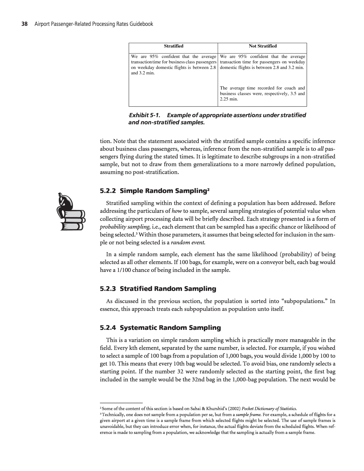
Sampling Techniques for Airport Data Collection 37 5.1.2 Scientific and Convenience Samples A scientific sample employs random selection to control for bias. A convenience sample, by con- trast, is one characterized by the relative availability of the sample elements. For example, assume that your goal is to sample 50 passengers going through security screening, and your plan is to record the amount of time each passenger took to complete screening. The recommended approach would be to use some random method of selecting the 50 passengers you observe, such as systematic random sampling (see Section 5.4.2). To save time, however, you decide to time the first 50 people in line. The following are biases this method might introduce: • The passengers at the front of the line likely arrived earlier than those at the end of the line, and, as such, might be different in some meaningful way, such as being better prepared, or, by contrast, people who do not often fly. • If the people at the front of the line are more experienced trav- elers, they may proceed more quickly, knowing the “drill.” • Vacationers who travel infrequently, however, and arrive well in advance of the flight’s depar- ture, may be less savvy and, as such take more time going through security. 5.1.3 Defining the Population While defining the population of interest might appear to be so pedestrian a subject as not to warrant formal attention, experience shows that this critical first step is often not properly done. It can be tricky as well. For example, an airport director charges you with the following task: “Find out what the average transaction time is for business class check-in on domestic flights during weekday mornings.” While the task seems reasonably straightforward, it begs a fun- damental question, i.e., what is driving the request for the data? Is the director interested in assessing performance against quality goals? Is he or she considering installing a new technology for check-in processing, or might the underlying reason be a question about the utility of adding staff during that time period? Determining the specific impetus might impact how the population from which the sample is drawn is defined. It might impact, for example, where data will be collected, whether parties or individual passengers will be observed, etc. The director’s charge also suggests several potentially meaningful differences. The wording implies that business class differs from other classes of flight, domestic differs from international, weekdays differ from weekends, and mornings differ from other times of the day. If these dis- tinctions are meaningful, the implication is that there is less variation in transaction time within each of these groups than there is between or among the groups. If this is the case, it argues for using a stratified sampling approach. The benefit is that it enables the researcher to make specific generalizations for each group such as, for example, being able to comment on the average trans- action time for business class passengers. 5.2 Sampling Strategies 5.2.1 Stratified Sampling Exhibit 5-1 is an example of the impact of stratified and non-stratified sampling on assertions that can justifiably be made. This assumes that stratification has been done prior to data collec- To reduce bias, use tactics that maximize randomness. Defining the research question helps to define the population to be studied.

38 Airport Passenger-Related Processing Rates Guidebook tion. Note that the statement associated with the stratified sample contains a specific inference about business class passengers, whereas, inference from the non-stratified sample is to all pas- sengers flying during the stated times. It is legitimate to describe subgroups in a non-stratified sample, but not to draw from them generalizations to a more narrowly defined population, assuming no post-stratification. 5.2.2 Simple Random Sampling2 Stratified sampling within the context of defining a population has been addressed. Before addressing the particulars of how to sample, several sampling strategies of potential value when collecting airport processing data will be briefly described. Each strategy presented is a form of probability sampling, i.e., each element that can be sampled has a specific chance or likelihood of being selected.3 Within those parameters, it assumes that being selected for inclusion in the sam- ple or not being selected is a random event. In a simple random sample, each element has the same likelihood (probability) of being selected as all other elements. If 100 bags, for example, were on a conveyor belt, each bag would have a 1/100 chance of being included in the sample. 5.2.3 Stratified Random Sampling As discussed in the previous section, the population is sorted into “subpopulations.” In essence, this approach treats each subpopulation as population unto itself. 5.2.4 Systematic Random Sampling This is a variation on simple random sampling which is practically more manageable in the field. Every kth element, separated by the same number, is selected. For example, if you wished to select a sample of 100 bags from a population of 1,000 bags, you would divide 1,000 by 100 to get 10. This means that every 10th bag would be selected. To avoid bias, one randomly selects a starting point. If the number 32 were randomly selected as the starting point, the first bag included in the sample would be the 32nd bag in the 1,000-bag population. The next would be Stratified Not Stratified We are 95% confident that the average transaction time for business class passengers on weekday domestic flights is between 2.8 and 3.2 min. We are 95% confident that the average transaction time for passengers on weekday domestic flights is between 2.8 and 3.2 min. The average time recorded for coach and business classes were, respectively, 3.5 and 2.25 min. .Exhibit 5-1. Example of appropriate assertions under stratified and non-stratified samples. 2 Some of the content of this section is based on Sahai & Khurshid’s (2002) Pocket Dictionary of Statistics. 3 Technically, one does not sample from a population per se, but from a sample frame. For example, a schedule of flights for a given airport at a given time is a sample frame from which selected flights might be selected. The use of sample frames is unavoidable, but they can introduce error when, for instance, the actual flights deviate from the scheduled flights. When ref- erence is made to sampling from a population, we acknowledge that the sampling is actually from a sample frame.

bag 42, then bag 52, and so forth. In October 2008, Washington, D.C., Metro announced that Transit Police would begin randomly searching riders’ bags using such a system. 5.2.5 Cluster Sampling Clusters are groupings of units, such as flights, gates, or terminals. Cluster sampling is used when it is difficult to define a formal list of elements (for example, a list of all passengers arriv- ing at an airport in a given time period) from which one could draw a random sample. However, since each arriving passenger must enter the airport at a gate, one could group pas- sengers into clusters by gates. In this instance, a random sample of gates would be drawn, and the characteristics of all arriving passengers exiting those gates would be collected. This is known as a one-stage approach. (Additional information about cluster sampling is included in Appendix C). 5.2.6 Time Periods as Sampling Units As noted previously, in order to assign a measure of data reliability to a sample, each unit must have an equal (or at least known) chance of being included. Since there are often many instances where a list of items cannot be obtained, another method might have to be employed. The fol- lowing case study is an example of a survey where a sample frame of flights may not be the opti- mal way of efficiently collecting data. Time Periods as Sampling Units—Case Study At one airport, there has been a desire to estimate the average time between a flight’s arrival at the gate and the appearance of its first bag on the bag claim carousel. This data is to be col- lected in such a way as to make inferences not only for the airport as a whole, but by airline and concourse. The first year, a stratified random sample of arriving flights was drawn and data col- lectors were assigned to “meet” the flight to record its arrival time and then proceed to bag claim to watch for its bags at the assigned carousel. While this method appeared to be a sound approach, in practice, it resulted in many missed flights and resurveys. This is because flights often reached the gate before their scheduled arrival time, much later than their scheduled arrival time, or at a gate different from the one listed on the monitor. To overcome these challenges, a different sampling approach was used—that of making time periods a sampling unit. In this example, a 7-day survey period was divided into 126 1-hour time periods (7 days × 18 hrs per day—for practical reasons, only hours that had at least two percent of the day’s arrivals were included) producing a sample frame. Then using proportional sam- pling, the probability of drawing a particular 1-hour time period during the week would be the same as the percentage of arriving flights scheduled to arrive during that same 60-min period. Separate sub-frames for each concourse/airline were drawn, creating a stratified sample. A ran- dom sample of concourse/time periods was then drawn. During the selected hour, the data col- lector could proceed to the concourse and wait for the next aircraft to come in. The data from that flight would then be included in the database. The result of using this method was that there was significantly less makeup work due to missed flights. 5.3 Sampling Steps The following is an overview of the principal steps (see Exhibit 5-2) involved in designing a sample. While the steps are presented in sequence, experience shows that the steps are often iter- ative and the process dynamic. Sampling Techniques for Airport Data Collection 39

40 Airport Passenger-Related Processing Rates Guidebook 5.4 Error Error in research is the difference between what actually is (i.e., its true state), and what it is reported to be true. While error is inevitable and impossible to eliminate, some error can be reduced. Broadly, there are two types of errors: random error and system- atic error. Random error is generally attributed to chance alone, whereas systematic error reflects inadequacies in how data are col- lected. If a regularly traveled flight took an average of 75 min, for example, sometimes it will take a little longer and on other occa- sions it will take less time. To an extent, the difference between the actual duration of the flight and the average (what is expected) is due to chance. Consider doing the following when first collecting data: 1. During the pilot (see Section 5.4.2), collect a small amount of data (e.g., 20 observations); 2. Perform a rough calculation of the mean and standard deviation. (If you plan on reporting frequencies see Section 5.4.3). Sampling Design Step Examples Comments 1. Define the population Domestic passengers checking-in during peak weekday mornings in autumn. If you wish to generalize to specific groups, consider using a stratified sample. (See Section 5.1.3.) 2. Define sampling units Individual passengers who obtain a boarding pass. A sampling unit is that which is counted or measured. 3. Define what is to be reported. Count of the number of passengers obtaining a boarding pass. Average time to complete a transaction. When reporting frequencies and averages, different formulas are used. (See Section 5.4.3.) 4. Identify the level of error you can tolerate. The sample count should be plus and minus 5 persons of what is the true (and unknown) population count. The sample average should be plus and minus 20 seconds of the true population average. This is a measure of precision. It reflects the width of the confidence interval. (See Section 5.4.3.) 5. Specify the desired level of confidence. We wish to be 95 percent confident. By convention, confidence levels range between 90% and 99%, with 95% being the most common. (See Section 5.4.5.) 6. Estimate the variance in the population. Population data always vary to some extent. (See Section 5.4.2.) 7. Estimate the required sample size. This is an iterative process. While one cannot change the observed or estimated variance in a population, one can manipulate confidence levels and tolerable error. 8. Select sampling strategy Simple random sampling. Stratified random sampling. Exhibit 5-2. Steps to sample design. Random error is inevitable, but systematic error can be reduced through careful plan- ning and execution.

3. If the standard deviation appears to be relatively large (as a rule of thumb, consider it large if it is 10 percent or more of the average value), ask yourself if there is something similar about those observations that were particularly large or small. For example, do the longer transac- tion times seem to be associated with party size or number of checked bags? Did the relatively brief transaction times seem to be related to persons apparently traveling on business? Granted, this distinction may not be verifiable, but if you think there may be a pattern, or something that helps explain variation, incorporate it into your sampling plan by recording the distinguishing information. Using the examples above, for example, might suggest that party size be recorded, while the number of checked bags might be ignored, or that the sus- pected purpose of travel (e.g., business or pleasure) be documented. 4. If the questions just asked both had affirmative answers, for example, consider capturing one more piece of data—whether the passenger appeared to be on business or pleasure travel. 5.4.1 Systematic Error Systematic error can be attributed to one or more causes, and often those causes are within the researcher’s ability to detect and correct. Exhibit 5-3 on the following page presents common reasons for systematic error, and proposes ways of avoiding such errors. 5.4.2 Calculating Error Variance is a measure of the average dispersion around a mean.4 How does one estimate the population variance? Sometimes, but not usually, the population standard deviation is known. Square it and you have the variance. When this unusual situation does not exist, there are sev- eral approaches to developing the estimate. 1. A previous similar study may have been conducted, and the variance calculated in that study could be used. 2. A small pilot study could be conducted, and the variance calculated from those data could be used. 3. If nothing is available, select a conservative value based on judgment and a very limited amount of data. For example, if the average time passengers wait in line is 4 min, you could conservatively guess that the standard deviation is the relative large value of 3 min. If this approach is taken, you can test your guess by calculating the actual standard deviation and variance for the real data. 4. Another approach, as described by van Bell is to make approximately 15 observations and then divide the range by the number of observations, an approach that is sufficiently robust to accommodate distributions both normal and substantially different from normal, (e.g., uniform). 5.4.3 Variance Steps 4, 5, and 6 in Exhibit 5-2 concern the amount of error one is willing to tolerate, the con- fidence one wishes to have, and variance in the population. Each of these issues needs to be con- sidered to calculate sample size. In particular, consider if and how the data’s level of measurement influences what is and is not permissible to calculate, and whether you are using a point esti- mate or a confidence interval approach. These topics are consid- ered in some detail in Appendix C. 4 Additional information on the topic of variance is included in Appendix C. The standard deviation is the square root of the variance. Sampling Techniques for Airport Data Collection 41

42 Airport Passenger-Related Processing Rates Guidebook 5.4.4 Confidence Levels & Hypothesis Testing Researchers often specify a research hypothesis, or a statement of the way the researcher believes things to be, and a null hypothesis. The null hypothesis is what is tested. The null hypothesis essentially asserts that there is no relationship between the variables. For example, if you sus- pected that, on average, people spent less time in check-in using kiosks rather than transactions with agents, you might state the hypotheses as follows: Research Hypothesis: On average, people spend less time in kiosk transactions than in agent transactions. Null Hypothesis: On average, people spend the same amount of time or more time in kiosk transactions than in agent transactions. A given confidence level reflects the probability of rejecting the null hypothesis when in fact it is true. It is customarily set at 0.95, meaning that the researcher is 95 percent confident in a decision to reject the null hypothesis. Rejecting a null hypothesis which is in reality true is referred to as Type I error. Exhibit 5-3 presents an example of how these error types might arise in an Airport environ- ment. Here, the decision to expand an airport facility is based on anticipated growth in demand. One cannot know with certainty what will happen in the future, the “true” state, but one can hypothesize and decide that growth will or will not occur. In two of the four possible combina- tions, the decision is accurate. The other two combinations, however, represent error. In this instance, a Type I error occurs when it is hypothesized that there will be growth, but it does not happen. The result is an increase in debt but not in revenue. If there is growth, however, but the decision is that growth will not happen and, as such, the facility is not expanded, the conse- quences might be missed revenue, a decrease in customer service, etc. Power is the other side of the confidence level issue. Power reflects the probability that one rejects the research hypothesis when indeed it is true. This is also known as a Type II error. 5.4.5 Tolerable Error This is the amount of error one is willing to tolerate in the sample estimate. For example, you might assert that the true average time spent in kiosk transactions is equal to the calculated sam- ple mean, plus or minus a given amount of time. If the time were equal to one minute, for instance, you could state, “95% confidence that the true population mean is equal to the sample mean of 4.5 min plus or minus one min.” The “True” State Decision No Growth Growth No Growth Correct Decision (Do not expand) Type II error (missed revenue, missed opportunities, customer service is a choke point, etc.) Growth Type I error (straddled with debt & no revenue) Correct Decision (Expand) Exhibit 5-3. Type I and type II errors, aviation example.

5.4.6 Random Error There is always some inherent amount of unexplained variation in what is observed. Not every person takes precisely 4.5 min to complete a transaction, nor will every registered Democrat vote for a Democratic candidate in an election. While one can’t control for this variation, it is impor- tant to estimate it when planning for sample size. 5.4.7 Trading Benefits and Costs In a perfect world, resource constraints would not be a problem. As such, one could minimize the possibility of making an error in incorrectly rejecting the null hypothesis, or incorrectly fail- ing to reject the null hypothesis when it is indeed true. Given the reality of a resource-constrained world, what criteria might you use to weigh the benefits of a larger sample against its cost? It is proposed that you weigh the potential consequences of each type of error. Whereas, for example, a five percent risk of a key part failure would not be acceptable, an error rate of five per- cent is assessing passenger satisfaction might be acceptable. Unfortunately, there are no absolute rules. Customarily, an error of five percent is acceptable in many of the sciences. Formulas and additional detail are included in Appendix C, and there are numerous websites that provide basic sample size calculators. 5.5 Calculating Sample Size5 This section offers guidance on how to calculate sample size for reporting proportions and means. As noted elsewhere, the approach for calculating sample size for simple random samples may, under certain conditions, be used for systematic and stratified sampling. In particular, for sys- tematic random sampling, the order of elements from which the sample is drawn must be random, and, assuming poststratification is not used, each stratum is treated as a separate population. The flow diagram presented as Exhibit 5-4 identifies some key questions and issues associated with the sample design. The formulas presented in this section will yield appropriate sample size calculations for both proportions and means (see Exhibits 5-5 through 5-8). They are appropriate, as well, for system- atic random samples assuming that the sampling elements from which the sample is drawn are randomly ordered. Situations in which one cannot assume such random ordering is beyond the scope of this guidebook. One text describes it as “. . . a formidable problem.”6 5.5.1 Calculating Sample Size When Reporting Proportions When proportions are to be reported, you need to estimate the incidence of the event in the pop- ulation, specify the level of error you are willing to tolerate, and identify the desired confidence level. Example In planning for redesign of a passenger check-in area, an airline is considering redesigning the space to better meet the demands of an increasing number of international passengers.7 5 The formulas presented are for determining approximate rather than exact estimates insofar as they do not require knowl- edge of the size of the population (N). The formulas presented assume that the population is sufficiently large and can be treated as an infinite population. When working with relatively small populations, a finite correction factor needs to be used to compensate for not replacing the sampling units. 6 Levy, P. & Lemeshow, S. (1999). Sampling of populations: Methods and applications. NY: Wiley. 7 For the purposes of the example, assume that these data are not available elsewhere. Sampling Techniques for Airport Data Collection 43

n = (1.962)(0.30)(0.70) 0.052 Exhibit 5-7. Example of determining sample size for reporting proportions. 44 Airport Passenger-Related Processing Rates Guidebook If the proportion of international passengers exceeds 30 percent, renovation will be initiated. The project sponsors indicate that they would like to be 95 percent confident that the propor- tion observed in the sample is +/− 0.05 (five percent) of the true population proportion. In Exhibit 5-7, the value 1.96 is used to represent the 95 percent confidence level. (Referring to Exhibit 5-6, note that where the desired confidence level is set at 99 percent, the value 2.58 would be used.) The proportion of international passengers that would trigger renovation is 30 percent. Hence, p is set at 0.30; 1 − p therefore must be 0.70. Finally, the numerator repre- sents the tolerable error. Solving the equation suggests a sample size of 323. Using this sample size would permit the researcher to assert, “we are 95 percent confident that the true proportion of international passengers is plus or minus 5 percent of the proportion observed in the sample.” Had the confidence level been set at 99 percent, the required sample size would have increased to 559. When calculating sample size for a proportion, do the following: 1. Trade off desired rigor and cost constraints by modifying the confidence level and/or the amount of tolerable error. First, change the error level and then, if necessary, change the con- fidence level. 2. If you have no basis for estimating the proportion, set p as 0.50. Outcome Variable ? Categorical Reporting Percents Continuous Reporting Means Sampling Design ? Simple or Systematic Random Stratified Cluster Analysis Compare 1 Sample Stats. to Pop. Compare 2+ Stats. Correlation Exhibit 5-4. Flow diagram. n = Z2p(1 – p) e 2 n = sample size. Z = the level of confidence desired (see Exhibit 5-6). p = the estimated proportion of what you wish to sample that is present in the population. 1 – p = the estimated proportion of what you wish to sample that is not present in the population. e = the level of error one is willing to tolerate. Exhibit 5-5. Formula to determine sample size when reporting proportions. Confidence Level Z value 90% 1.645 95% 1.96 99% 2.58 Exhibit 5-6. Confidence level and corresponding Z values.

5.5.2 Calculating Sample Size When Reporting Means (Averages)8 When means are to be reported, the estimated variance, rather than the estimated proportion, is used in the calculation. Use the formula in Exhibit 5-8 when conducting a simple random sam- ple with the intent of reporting averages. The structure is identical to the formula in Exhibit 5-5. Example An airport is interested in determining the average transaction time for domestic passengers interacting with an agent during check-in. The project sponsors would like to be 95 percent con- fident in the estimate (sample average) obtained from the sample. In addition, they would like the estimate to be within five seconds (error) of the true population mean. Given: Z = 1.96 e = 5 seconds σ = 35 seconds The sample size is calculated to be 188 transactions. Thus far, essentially the same information needed for the proportion formula exists. What is missing is a measure of variation. In the proportion formula, variation was operationalized as an estimate of the proportions in the population. When using the formula for calculating sample size when averages are to be reported, another estimate must be used, namely, the variance. For the moment, where the variance estimate comes from will be ignored. Appendix C contains information for calculating sample size when assessing change, examining relationships, situations involving varying sample costs, and when testing for differences in averages. 5.6 Determining When to Schedule a Data Collection Event One characteristic of a good sample is that it is a fair approximation of the population it rep- resents. This pertains not only to entities but to time periods. For example, were you to choose the late afternoon and early evening on December 23 to collect data on passenger processing rates at Chicago O’Hare International Airport, it would obviously give you very different results com- pared to those obtained on a Monday morning in September. Sampling Techniques for Airport Data Collection 45 n = Z2σ2 e 2 n = sample size. Z = the level of confidence desired. σ2 = the Greek letter sigma. Sigma squared is referred to as variance. Similar to p and 1 – p in the formula for proportions, the variance is a measure of dispersion (random error), or unexplained variance in the distribution. e = the level of error one is willing to tolerate. Exhibit 5-8. Sample size formula for reporting means. 8 vanBell, G. Statistical rules of thumb. (2002), NY: Wiley.

Airport passenger-related activity varies by season/month of the year, day of the week, and time of day. For this reason, it is important to give consideration to the scheduling of your data collection event(s). Generally, it is best to collect data during a peak period for the following two reasons: 1. Most planning is focused on providing adequate peak hour capacity; 2. A queue and constant demand for resources are required to calculate processing times. While there is some variation in defining peak periods across functions, the commonalities are much stronger. As such, determining peak periods from a general perspective is considered, noting, as appropriate, differences unique to specific functions. As shown in Exhibit 5-9, the aviation industry has many sources of data that, while not per- fect, are considered useful for determining peak periods of activity. Independent of breadth of time for which you are interested in determining a peak period, the following are basically only two sources to go to for help: • Data—presumably “objective” in how it was captured, and likely collected for another pur- pose; and • People—from whom subjective insights and judgments are solicited. 46 Airport Passenger-Related Processing Rates Guidebook Peak Busy /Peak Peak Sourc e M onth Day Hour Ai rp or t Mg t. Statistic s --Landing Repor ts X --Monthly Activit y Stats . X --Par ki ng Counts (1 ) X X X --Roadway Tr af fi c Counts (2 ) X X X U.S. DOT T- 100 X Official Ai rline Gu ide (3) X X X (OAG) TS A Wait Time Data (4) X Informant (5 ) --Loc al Airline Station Mgrs. X X X X --Loc al T SA Manager X X X --Loc al US CBP Manager X X X Notes : ( 1) Prim arily re fl ect tr avel patterns of residents. (2) Road wa y counts can be affected by other activity centers (e.g., nearby construction area or employee parking lot). (3) Must also account for load factor variation and percent originations . (4) From T SA website (www.tsa.gov/traveler s/ waittim e.shtm ); high wa it tim es ma y not only be due to peak dem and but insu ffi ci ent sta ffi ng . (5) Inform ants can pr ovide both proprietar y, quantitative re cords and qualitative/anecdotal input; the latter should be used with caution. Sources to Determine Peak Periods Exhibit 5-9. Sources determining peak periods of activity.

People, the latter source, are sometimes formally referred to as informants: persons with knowledge specific to a unique situation. Consider informants as a potentially valuable source of data. (For more guidance on using informants, see Section 5.8.) The next section provides guidance on how to establish an airport’s peak month, busy day, and peak hour, including which data sources to use and how to use them effectively to determine peak periods for your particular area of interest. 5.6.1 Identifying the Peak Month In general, most functional elements that are typically examined for an airport processing rate study tend to have a common peak month. (This should be verified for your airport, however.) The following sections provide discussion of the usefulness of various databases to determine the peak month. Airport Management Statistics Nearly every airport with scheduled passenger service keeps records of monthly passenger and aircraft activity. These reports, most commonly prepared by the finance department, are avail- able from airport management or from the airport’s web-site. Collected by the airlines, they include monthly data related to passenger enplanements and deplanements, freight and mail tonnage, and aircraft landings and takeoffs. Domestic and international activity may be collected separately. It is recommended to use these statistics for determining the peak month for overall passenger and aircraft operations activity using the process described below. To determine the peak month, review monthly activity data for the most recent 3-year period. In general, the peak month occurs in the summer. For some markets, however, particularly vaca- tion destinations such as Orlando, the peak may occur in the spring or other time of the year. Exhibit 5-10 shows average daily enplanements by month at Washington Reagan National Airport for 2007. As shown, June was the peak month. The following is an evaluation of other various sources for peak month data. Sampling Techniques for Airport Data Collection 47 0 5,000 10,000 15,000 20,000 25,000 30,000 35,000 Jan Feb Mar Apr May Jun Jul Aug Sep Oct Nov Dec Month A ve ra ge D ai ly P as se ng er s Source: Metropolitan Washington Airports Authority; HNTB analysis. Exhibit 5-10. Average daily departing passengers by month at Reagan National Airport, 2007.

U.S. DOT Form 41 Data/T100 These data report monthly traffic data by carrier and city-pair and can be used to determine peak month activity. Origin-Destination Data These data represent a 10 percent sample of aviation activity (both passengers and cargo). The benefit of Origin-Destination (O&D) data is that it excludes connecting traffic. However, there are several disadvantages. First, while they represent actual passenger origins and destinations, they are prone to error due to inaccurate/incomplete reporting by the airlines; however, this can be largely overcome by obtaining the data from a third party source that rectifies and “cleans” the data—although at a cost. In addition, O&D data are only available by quarter, not by month, so they can only be used to get a general sense of when an airport is busy. Official Airline Guide The Official Airline Guide (OAG) is the sole database of all scheduled commercial airline flights worldwide. Typical OAG data include published and scheduled operator (airline), air- craft type, seats, scheduled arrival and departure times, origin and destination (and downline stops), and effective/discontinued dates. A sample raw schedule pull from OAG is shown in Exhibit 5-11. OAG data can only be used to examine trends in scheduled activity and only of flights and seats. While in general, airlines schedule more flights and seats during busy periods, competitive pres- sures, aircraft positioning requirements, and other factors can sometimes distort when peaks occur. OAG data can also be useful for very short-range forecasts of activity—up to six months. Beyond that, the level of uncertainty increases significantly. The cost of a “schedule pull” varies in a largely linear fashion by the number of fields included and the number of records, so that a schedule pull for a large commercial airport can be signif- icantly more expensive than for a less busy airport, costing several thousand dollars. For addi- tional information, contact an OAG customer service agent or sales manager at (630) 515-5300 or at custsvc@oag.com. Note that the OAG is potentially useful in identifying peak days and hours as well. Other Sources The airlines, TSA, and CBP collect passenger activity data and therefore have historic infor- mation to help determine peak periods or to serve as a back-check for surveyed data. However, unless the study is being conducted for the particular entity, it is unlikely they will share propri- etary or security-related information. Finally, there is usually an abundance of anecdotal information that comes from talking with airport staff, on-site government agencies, and tenants (informants). As noted elsewhere, be cautious and seek confirmation or disconfirmation from multiple persons. 48 Airport Passenger-Related Processing Rates Guidebook carrier fltno depapt arrapt arrctry deptim arrtim days genacft inpacft seats domint efffrom effto sad acft_owner DL 5113 ABE ATL US 0600 0800 1 CRJ CRJ 50 DD 20080707 20080707 OH OH DL 4171 ABE ATL US 0630 0836 1234567 CRJ CRJ 50 DD 20080616 20080706 EV EV DL 4171 ABE ATL US 0630 0836 1234567 CRJ CRJ 50 DD 20080708 20080727 EV EV DL 4171 ABE ATL US 0630 0836 1234567 CRJ CRJ 50 DD 20080729 20080818 EV EV DL 4171 ABE ATL US 0650 0856 1234567 CRJ CRJ 50 DD 20080819 20080901 EV EV DL 4915 ABE ATL US 0650 0856 1234567 CRJ CRJ 50 DD 20080902 20090615 EV EV Copyright 2008, OAG Worldwide LLC All Rights Reserved. Exhibit 5-11. Sample OAG “schedule pull” database.

5.6.2 Identifying Peak Days At the daily level, a distinction should be made between departing and arriving passengers. The researcher should therefore decide whether his or her area of focus is largely driven by departing passengers (e.g., airline check-in and security), arriving passengers (e.g., FIS or bag claim), or a combination of the two (e.g., curbside activity). Exhibit 5-12 shows day-to-day local departing and arriving passenger activity at Hartsfield-Jackson Atlanta International Airport over a one-week period in late June 2008. As shown, the peak day for departing passengers was Thursday, while the peak day for arriv- ing passengers was Monday. Determining peak days of the week is more difficult than determining peak months because most readily-available sources do not typically keep data on a daily basis. The data above were obtained by a one-week survey at the entrances and exits to the airport’s secure areas. In most instances, time and resource constraints will preclude you from obtaining this type of data. The optimal way of obtaining daily counts of passengers would be to obtain historical data from local airline station managers and/or local TSA or CBP officer. But, as noted in the previ- ous section, they may be unwilling to provide this data. They may be willing, however, to review their data themselves and provide general guidance. An examination of OAG data by day can be useful; however, as noted previously, there are competitive and operational factors that tend to mute day-to-day schedule variations. (For example, on a typical weekday, airlines will have to schedule the same number of departing flights as arriving flights, even though on any given weekday there may be more outbound pas- sengers than inbound passengers, historically.) One can also examine TSA wait time data, which is available on their website. One can choose an airport, day of week and hour of the day, and the average and maximum wait time at various Sampling Techniques for Airport Data Collection 49 0 10 20 30 40 50 60 70 80 Sun Mon Tue Wed Thu Fri Sat Pa ss en ge rs (0 00 s) Source: Hartsfield-Jackson Atlanta International Airport 2008 Peak Week Survey; HNTB analysis. (1) Counts of people entering and exiting secure side of airport, respectively. Dep. Arr. Exhibit 5-12. Counts of originating and terminating passengers by day of week in June 2008 at Hartsfield-Jackson Atlanta International Airport.

checkpoints will be displayed. Assuming that the days with the highest wait times are the busiest, a busy day can be identified. (It should be noted, however, that high wait times may also be the result of insufficient staffing at the checkpoint.) 5.6.3 Defining Peak Hours As with peak day activity, peak hour activity at various functional elements will be largely determined by whether it serves primarily departing passengers, arriving passengers, or both. Exhibit 5-13 shows hourly counts of local departing and arriving passengers on a Wednesday in early July 2008 at Hartsfield-Jackson Atlanta International Airport. As shown, local departing passenger activity peaked early in the morning (between 6 a.m. and 10 a.m.); a secondary departing passenger peak occurred in mid-afternoon. For arriving passen- gers activity was generally low until about 2 p.m. The peak for arriving passengers occurred between 7 a.m. and 9 a.m. Sources of Hourly Data As with day-of-week data, the optimal sources for hourly data include local airline station managers and TSA. Again, however, there will likely be a reluctance to share this type of data, leaving the researcher with less-than-optimal sources. One could examine TSA checkpoint wait time data, which are available on their website; how- ever, as noted previously, delays may be due to insufficient staffing. An OAG schedule pull of departing and arriving aircraft and seats will be of some benefit. A caution should be noted here in that, for airports with significant amounts of connecting pas- senger activity, an hour-by-hour of summary of seats will show multiple peaks across the day, directly corresponding to the “banks” of flights operated by the hub airline. This will make it dif- ficult to pick the bank or banks with the most local passengers (if the element of study is in fact primarily affected only by local passengers). Nevertheless, as there are really no other readily-available data sources, an OAG schedule pull is often the best source. 50 Airport Passenger-Related Processing Rates Guidebook 0 1 2 3 4 5 6 7 8 5 76 8 9 10 11 12 13 14 15 16 17 18 19 20 21 22 Pa ss en ge rs (0 00 s) Hour of Day Dep. Arr. Exhibit 5-13. Hourly distribution of local departing and arriving passengers at Hartsfield-Jackson Atlanta International Airport on Wednesday, July 2, 2008.

Using an OAG Schedule Pull to Determine the Peak Hour for Various Functional Elements At the outset, it must be understood that the published times listed in an OAG schedule pull are the times when a flight is scheduled to depart or arrive. If the peak hour for departing seats is between 8 a.m. and 9 a.m., do not assume that this is when you should be collecting data at ticketing, for example, because passengers will already be at the gate boarding their flights. Rather, adjustments must be made to the OAG schedule to anticipate when particular functional elements will peak in activity as described below. Adjustments to Departing Seat Schedule Exhibit 5-14 shows the cumulative percentage of local passengers arriving at a terminal by hours and minutes before their flight is scheduled to depart. The information comes from actual survey data collected from one small, regional east coast airport and one large, international east coast airport in the fall of 2005. Patterns at other airports may vary from those presented here. Note that the time interval is strongly influenced by whether a passenger is traveling on a domestic or international itinerary and if the flight is leaving early in the morning; therefore, sep- arate exhibits are provided for these scenarios. In addition, each graph also shows separate curves for data gathered at a large international airport and a small/regional airport; a median curve (dotted line) is also provided. In general, passengers tend to allow less time for making their flight early in the morning, when traveling domestically, and at small airports. Conversely, passengers Sampling Techniques for Airport Data Collection 51 0% 10% 20% 30% 40% 50% 60% 70% 80% 90% 100% 3:20 3:00 2:40 2:20 2:00 1:40 1:20 1:00 0:40 0:20 0:00 Minutes before Scheduled Departure Time Sm all /R eg ion al Ai rp or t La rge Int er na tio na l A irp or t International Itinerary Flights Leaving Prior to 9:00 AM 0% 10% 20% 30% 40% 50% 60% 70% 80% 90% 100% 3:20 3:00 2:40 2:20 2:00 1:40 1:20 1:00 0:40 0:20 0:00 Minutes before Scheduled Departure Time Sm all /Re gio na l A irp or t La rge Int er na tion al A irp or t International Itinerary Flights Leaving After 9:00 AM 0% 10% 20% 30% 40% 50% 60% 70% 80% 90% 100% 3:20 3:00 2:40 2:20 2:00 1:40 1:20 1:00 0:40 0:20 0:00 Minutes before Scheduled Departure Time Sm al l/R eg io na l A irp or t La rge Int er na tio na l A irp or t Domestic Itinerary Flights Leaving Prior to 9:00 AM 0% 10% 20% 30% 40% 50% 60% 70% 80% 90% 100% 3:20 3:00 2:40 2:20 2:00 1:40 1:20 1:00 0:40 0:20 0:00 Minutes before Scheduled Departure Time Sm all /R eg ion al Ai rp or t La rge Int er na tio na l A irp or t Domestic Itinerary Flights Leaving After 9:00 AM Exhibit 5-14. Departing passenger time of arrival at terminal relative to scheduled departure time (cumulative).

52 Airport Passenger-Related Processing Rates Guidebook 0 100 200 300 400 500 600 0530- 0544 0645- 0659 0745- 0759 0845- 0859 0945- 0959 1045- 1059 1145- 1159 1245- 1259 1345- 1359 1445- 1459 1545- 1559 1645- 1659 1745- 1759 1845- 1859 1945- 1959 2045- 2059 2145- 2159 2300- 2314 15-Minute Time Period Se at D ep ar tu re s Rolling 60-minutes 90% of Hourly Peak Exhibit 5-15. American Airlines scheduled seat departures per 15-min increments, Hartsfield-Jackson Atlanta International Airport on July 18, 2007. tend to allow more time for processing when their flight leaves later in the day, when traveling internationally, and when using a large airport. For example, to estimate when the morning peak period would begin at the American Airlines ticket counter at Hartsfield-Jackson Atlanta International Airport, for example, plot out sched- uled seat departures (Exhibit 5-15). Note that these data reflect that the morning peak hour, in terms of seat departures, is between 6:15 a.m. and 7:15 a.m. Recognizing that most passengers are traveling on a domestic itinerary and that these flights are departing before 9:00 a.m., exam- ine the curve for a large international airport in Exhibit 5-14 to see that these passengers trav- eling under these conditions have a median time of arrival at the terminal of about 1 hour and 40 min. Therefore, the recommended time to begin the actual data collection would be 4:35 a.m. (It should be noted that the airline may not even open the counter until 5:00 a.m.; however, if one is measuring demand, it may be appropriate to begin monitoring at about 4:30 a.m. as that is when passengers will likely begin showing up.) A similar process can be used to estimate when peaks would occur at other terminal elements, depending on their location within a departing passenger’s flow through the terminal. For exam- ple, if one were looking at processing rates at a security checkpoint, one might slightly reduce the time factor assumed compared to those listed above, recognizing that this process is closer to a flight’s actual departure time. Adjustments to Arriving Seat Schedule Processes most closely related to arriving seat schedules include bag claim, restroom utiliza- tion, and FIS processing. As with departing seat schedules, those for arriving seats may need to be adjusted, albeit less dramatically. For instances, at a small airport, only 5 min may elapse between a flight’s arrival and the time its passengers reach a bag carousel. At a large airport, it might take 15 min before passengers reach bag claim. Adding a “Cushion” Lastly, it is wise to bracket your peak hour estimate by at least 30 min (preferably one hour) on either side. This will help reduce the chance of missing the peak—either because of a mis- applied assumption, inherent variability between scheduled times and actual times (particularly

with arriving flights), and because it gives you a chance to see and describe how a peak builds and wanes. Peak Hour Rules-of-Thumb There are many factors that affect when peaking occurs at airports; however, when there is a lack of data, the following rules of thumb might be useful to helping establish the peak hour for various terminal elements. While some of these are based on “hard data,” many are based on sur- veyor experience. 1. Local departing passenger activity peaks in the early morning at most airports. At hub airports, the busiest morning period in terms of departing flights is usually between 7 a.m. and 10 a.m. (resulting in ticketing and security activity peaking between 5 a.m. and 8 a.m.), while at spoke airports, the busiest morning period begins about one hour earlier—between 6 a.m. and 9 a.m. (resulting in ticketing and security processing peaking around 4:30 a.m. and 7:30 a.m.). 2. A second, more spread-out departure peak begins in the mid-afternoon and lasts through early evening. 3. Local arriving passenger activity is generally light until mid-afternoon, peaking in the early evening. 4. FIS selection of a time of day should be based on knowledge of when peak activity is antici- pated at the FIS facility. Historically, the traditional peak period for international arrivals has been the mid- to late-afternoon, reflecting the predominance of trans-Atlantic travel. Beginning in the 1980s, traffic between Asia began to grow rapidly. Since these flights typi- cally arrive in the late morning, United States airports with nonstop service to Asia also see international arrival activity increase at that time as well. In the 1990s, Central American and South American markets began growing at a faster-than-average rate. Peak arrival times for flights from these markets have a less definite diurnal arrival pattern. Overall, therefore, while the typical busy period at most FIS facilities remains the mid-afternoon, the geographic loca- tion of the study airport and the mix of international markets served by that airport require the researcher to examine actual schedules. 5. At O&D airports (i.e., those without a significant number of connecting passengers) or air- lines with only “spoke” service at hub airports, the peak hour for most functions can be deter- mined by examining the timing of scheduled seat departures (for check-in, security, and other departing passenger-related functions) and arrivals (for FIS, baggage claim, and other arrival- related functions) and making adjustments for the anticipated amount of time between a pas- senger’s reaching the terminal and the flight’s scheduled departure or arrival time. 6. For hub airports (and airlines with hub-type activity at the station of interest), actual local passenger (i.e., originating and terminating passengers) peaking activity it is more difficult to directly tie peaks in originating passenger activity to peaks in seat departures and arrivals (as might be obtained from an OAG schedule pull) because the percentage of connecting passen- gers will vary by bank. 5.7 Proxies for Absolute Peak While it is often desirable to gather data during the peak month or peak hour, there may be overall project scheduling or resource constraints that would make that impractical. In these instances, it is recommended to choose a time period with at least 90 percent of peak activity. Using the Reagan National monthly statistics as shown in Exhibit 5-16, one can see that six other months were at least 90 percent as busy as the peak month, June. It should be noted, however, that while the absolute number of passengers is similar to that seen in the peak month, passenger travel characteristics may be different, which could affect results. Sampling Techniques for Airport Data Collection 53

5.8 The Role of Informants This section looks at the role informants can play in helping not only determine when to schedule data collection events, but also in helping identify those factors that signal salient dif- ferences, or might help explain how entities, resources, and processes are different from one another and hence need to be recorded in data collection. To use a basic example, assume that your task is to estimate the average amount of time agents spend with customers. Passengers and their travel characteristics will differ in an infinite number of ways, but which attributes might be relevant in explaining how long passengers spend with air- line check-in agents? Gender, hair color, height, and so forth are obviously irrelevant, but what is relevant? To learn what is relevant requires knowledge and perspective that can only come from experience. Persons with such knowledge and experience are sometimes referred to as informants. An informant is a person who “knows what is going on” at a given airport, or a particular process at that airport, and is willing to share relevant information with you. 5.8.1 Example of Use of Informants The following, drawn from the experience of a member of the Research Team, illustrates the value of informants. Annually, international arriving passenger-related processing rate data are gathered at a particular busy airport during one day of the week in the peak month. Having col- lected these data over several years, and using anecdotal information as well as an analysis of scheduled seat arrivals, the researcher traditionally picked Saturday afternoons as a busy period. In preparation for this annual effort, he reviewed the scheduled seat arrival data for the week and day of interest and noticed that the peak had seemingly shifted from the afternoon to the early evening. Further, a review of TSA wait-time data at the international arrival checkpoint through which arriving passengers must pass prior to entering the domestic portion of the terminal showed significant delays on Thursday afternoons, suggesting that Thursday, not Saturday was the peak day for international arrivals. He was skeptical that Thursday would be a busy day for international arrivals, based on his assumption that most people would want to return from an international destination on a weekend. 54 Airport Passenger-Related Processing Rates Guidebook 0 5,000 10,000 15,000 20,000 25,000 30,000 35,000 Jan Feb Mar Apr May Jun Jul Aug Sep Oct Nov Dec Month A ve ra ge D ai ly P as se ng er s Source: Metropolitan Washington Airports Authority; HNTB analysis. 90% of Peak Exhibit 5-16. Assuming 90 percent of peak period activity is a way to expand survey opportunities.

To confirm that the day of the week and the time of day had shifted, the researcher discussed the seat arrival and TSA wait time data with a representative of the company that handles interna- tional flights at the airport. During the discussion he learned that the peak time of day had, in fact, shifted to early evening; however, the busiest days of the week were still Saturday and Sunday. The informant interpreted the longer wait times at the checkpoint on Thursdays likely to be a function of lower TSA staffing levels on Thursdays, and not reflective of a shift from the weekend. The researcher kept Saturday as the day of data collection, but shifted the time period into the evening to capture the new peak. 5.8.2 Summary While humans are proficient in making meaningful discriminations, there is a large body of research literature that people are also quite adept at inferring patterns when there are none. A related finding is that increased experience is often accompanied by an increase in self-confidence in the accuracy of judgments. For example, experienced law enforcement personnel will often be very confident in their ability to tell when someone is lying or telling the truth; unfortunately, their performance is usually about as poor as those with no experience—essentially equivalent to flipping a coin. In summary, it is strongly recommended to supplement “hard” data obtained from reports and databases with informants’ observations. Given human limitations, however, we recom- mend conferring with more than a single informant. Sampling Techniques for Airport Data Collection 55 Use informants; they can help you identify issues of which you may not even be aware, as well as verifying the accuracy of what you have learned through other sources (e.g., past reports, databases).