Access Management in the Vicinity of Interchanges, Volume 2: Research Overview (2022)

Below is the uncorrected machine-read text of this chapter, intended to provide our own search engines and external engines with highly rich, chapter-representative searchable text of each book. Because it is UNCORRECTED material, please consider the following text as a useful but insufficient proxy for the authoritative book pages.

31   Efficient traffic operations for crossroads in the vicinity of interchanges can be largely impacted by traffic maneuvers into and out of driveways or public intersections. To assess the operational performance of the study sites, the project team collected field data (including traffic volumes at each driveway) and used this information to develop micro-simulation models (using VISSIM) for each site. The project team used field-collected travel time information to validate the VISSIM models. The following sections summarize the field operational study and the micro-simulation model (model development, model validation, and scenario development) as well as operational analysis findings and statistical analysis of VISSIM speed data. Field Operational Study The project team evaluated each study location to identify unique operational configurations, general operational trends, and items of concern that could adversely affect the use of a site for subsequent analysis. The team collected traffic volumes for peak and off-peak time periods, recorded travel times during these evaluation periods, and monitored the length of queues at the intersections and driveways. Ultimately, the queue length data did not provide any meaningful results and was not included in this report; however, the conflict study reviewed in Chapter 5 did consider the influence of queue for operations related to safety. The evaluation of prevailing speeds and volumes at each location enabled the project team to extend the research into a micro-simulation analysis where varying scenarios could be systematically evaluated for operational performance. The following sections review this micro-simulation analysis task. Micro-Simulation Model The use of micro-simulation for an enhanced operational analysis enables the evaluation of key features that may not be present at a location in a configuration that will provide meaningful results. For example, evaluation of the influence that the proximity of a downstream, signalized intersection can have on corridor operations can be enhanced by using a validated simulation model and then varying the distance of interest. To use micro-simulation for this purpose, the project team first had to develop realistic simulation models that represented field con- ditions and then validate the performance of the models to ensure they adequately captured observed field conditions. The model development and validation efforts are described in the following sections. C H A P T E R 4 Operational Analysis

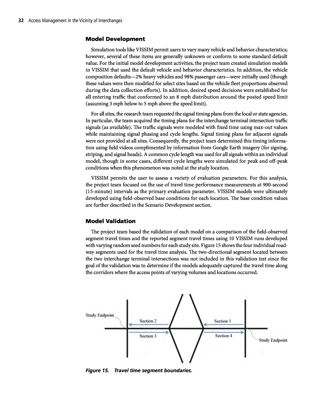
32 Access Management in the Vicinity of Interchanges Model Development Simulation tools like VISSIM permit users to vary many vehicle and behavior characteristics; however, several of these items are generally unknown or conform to some standard default value. For the initial model development activities, the project team created simulation models in VISSIM that used the default vehicle and behavior characteristics. In addition, the vehicle composition defaults—2% heavy vehicles and 98% passenger cars—were initially used (though these values were then modified for select sites based on the vehicle fleet proportions observed during the data collection efforts). In addition, desired speed decisions were established for all entering traffic that conformed to an 8 mph distribution around the posted speed limit (assuming 3 mph below to 5 mph above the speed limit). For all sites, the research team requested the signal timing plans from the local or state agencies. In particular, the team acquired the timing plans for the interchange terminal intersection traffic signals (as available). The traffic signals were modeled with fixed time using max-out values while maintaining signal phasing and cycle lengths. Signal timing plans for adjacent signals were not provided at all sites. Consequently, the project team determined this timing informa- tion using field videos complimented by information from Google Earth imagery (for signing, striping, and signal heads). A common cycle length was used for all signals within an individual model, though in some cases, different cycle lengths were simulated for peak and off-peak conditions when this phenomenon was noted at the study location. VISSIM permits the user to assess a variety of evaluation parameters. For this analysis, the project team focused on the use of travel time performance measurements at 900-second (15-minute) intervals as the primary evaluation parameter. VISSIM models were ultimately developed using field-observed base conditions for each location. The base condition values are further described in the Scenario Development section. Model Validation The project team based the validation of each model on a comparison of the field-observed segment travel times and the reported segment travel times using 10 VISSIM runs developed with varying random seed numbers for each study site. Figure 15 shows the four individual road- way segments used for the travel time analysis. The two-directional segment located between the two interchange terminal intersections was not included in this validation test since the goal of the validation was to determine if the models adequately captured the travel time along the corridors where the access points of varying volumes and locations occurred. Figure 15. Travel time segment boundaries.

Operational Analysis 33   Because peak and off-peak conditions could vary, the project team created models for both time periods and separately validated the resulting models. The field study travel time values are shown in Table 21. Column E represents examples of the average of all travel time runs conducted during the peak or off-peak hours accordingly (as determined by the traffic volume counts). The number of field runs ranged from one to 12. The segments were measured from center-of-intersection to center-of-intersection. Due to variations in the field-measured segment lengths compared to the values in the VISSIM models, the field values were adjusted slightly to account for the differences in distance (Column F). The VISSIM Average Travel Time (Column B) is the average travel time (based on 10 simu- lation runs) for all through vehicles traveling along the segment. VISSIM also provides the standard deviation of the travel times (Column C). The project team considered a model to be validated when the adjusted field study travel time was within two standard deviations (an estimate of a 95% confidence interval) of the VISSIM travel time (Column G ≤ Column D). It should be emphasized that the standard deviation values used in this validation effort are from the VISSIM model, not the field study. Because the VISSIM model results represent every vehicle traveling through the travel time segment (sometimes equivalent to more than 1,000 vehicles), the variability of the VISSIM data is significantly less than that of the field data with a much smaller sample size. Consequently, using the VISSIM standard deviation is a conservative approach. In cases where the VISSIM standard deviation was very small and valida- tion could not be simultaneously achieved on all four segments, the project team considered the model to be valid if three of the four segments validated using the above process. The process assumed that the remaining segment validated using the standard deviation of the field data. At a few sites, the hours of the travel time runs did not coincide with peak or off-peak traffic volumes, and thus travel time data was not available for validation of both sets of traffic conditions. The VISSIM models for two of the study sites did not successfully validate. The Phoenix, Arizona, roundabout site (Site AZ #6) and the Springfield, Missouri, diverging diamond (MO #1) did not successfully validate using the VISSIM models. This is likely due to differences in car following or lane distribution that are not directly accounted for using the conventional VISSIM default values. Scenario Development The validated VISSIM models for the various interchange study locations provide a base condition that can be varied to assess the influence of various access management features A B C D E F G VISSIM Travel Time Measurement VISSIM Average Travel Time (sec) One Standard Deviation (sec) Two Standard Deviations (sec) Field Study Average Travel Time (sec) Adjusted Field Study Average Travel Time (sec) Travel Time Difference (sec) 1 36.71 3.02 6.03 42 41.9 5.17 2 13.42 0.59 1.18 13 12.8 0.59 3 28.85 2.91 5.82 25 25.9 2.93 4 35.20 2.78 5.55 38 38.5 3.26 Table 21. Example travel time statistics used for VISSIM model validation.

34 Access Management in the Vicinity of Interchanges associated with the unique interchange configuration. The study scenarios must adhere to key practical constraints. For example, the volume can be incrementally increased for a STOP- controlled diamond interchange, but practical limits to the actual construction of this type of interchange must be considered. If, for example, a signal is warranted at a specific volume threshold then the simulation scenarios should not exceed this value. In most cases, a micro-simulation tool like VISSIM will achieve corridor saturation for high-volume or restrictive configurations, and this will result in “dropped” vehicles or spillback onto adjacent segments. Because this simulation state is not stable and so does not represent actual roadway configurations, it can also be considered an indication that study scenario limits are not valid. When this phenomenon occurred, the VISSIM scenarios were considered out of range and removed from the analysis. For the scenario development effort, the project team used the field-validated simulation models to assess how varying the following factors would affect corridor operations: • Volume (VISSIM uses an origin-destination matrix, but, for simplicity, the two-direction volume is shown in subsequent tables), • Distance to next major signalized intersection, • Density of access points, • Distance to the initial downstream driveway (DSDW) (departing the interchange), • Distance to the initial upstream driveway (USDW) (approaching the interchange), and • Median configuration. The project team evaluated peak and off-peak base conditions where available. Due to the large variety of site conditions, the VISSIM features available for base conditions differ considerably. The model scenarios, therefore, differ for each location. The following sections depict the models simulated for each of the validated study sites. Similar to the proce- dure described in the previous validation summary, the project team evaluated each scenario using average statistics from 10 simulations per scenario. Signalized Diamond Interchanges The signalized diamond interchange included locations with and without right-turn channelization. Table 22 summarizes the signalized diamond interchange scenarios without channelized right turns. Similarly, Table 23 depicts the scenarios with channelized right turns. Basic characteristics of the signalized diamond interchange simulation scenarios are described as follows: • Observed posted speed limits were 30, 35, 40, and 45 mph; • Median treatments included TWLTL; raised, continuous; and raised, strategic (to restrict select driveway access); • Base condition distances to the closest (non-interchange) signalized intersection were as small as 400 ft and as large as 2,640 ft (simulation scenarios ranged from 400 to 2,640 ft); • Base condition access spacing ranged from 17 up to 102 driveways per mile (DW/mi), and simulation scenarios were all within this range; • Distances to DSDWs varied from as close as 65 ft to as far as 610 ft from the terminal inter- section (simulation scenarios ranged from 0 up to 1,300 ft); • Distances to USDWs varied from as close as 100 ft to as far as 525 ft from the terminal inter- section (simulation scenarios ranged from 100 up to 1,300 ft); and • Field-observed two-way traffic volumes ranged from 700 up to 3,800 vph (simulation scenarios ranged from 700 up to 5,200 vph).

Operational Analysis 35   Site Posted Speed Limit (mph) Scenario Median Type Distance to Signal (ft) Access Density (DW/mi) Distance to DSDW (ft) Distance to USDW (ft) Signal Cycle Length (sec) Two- Way Volume (vph) AZ #1 (S) 35 Base TWLTL 1,100 58 275 135 95 1,300, 2,000, 2,300, 2,500 1 275 500 2 23 275 135 3 58 500 2004 150 500 5 23 500 2006 150 500 AZ #1 (N) 35 Base TWLTL None 70 125 525 95 1,750, 2,450, 2,750, 2,950 1 22 500 525 2 70 125 2003 500 525 4 22 125 2005 1,000 1,000 6 70 1,000 1,000 AZ #2 (S) 35 Base Raised, Strategic 700 23 200 400 130 850, 1,150, 1,450, 1,650, 1,750, 1,950, 2,050 1 Raised, Continuous 200 400 2 1,500 22 200 400 3 40 200 400 4 22 1,000 1,000 5 40 1,000 1,000 6 700 500 2007 200 400 AZ #3 (E) 45 Base Raised, Strategic 1,650 42 300 340 130 2,000, 2,500, 2,700, 3,000, 3,100, 3,700, 3,800, 3,900 1 19 500 200 2 19 300 340 3 19 1,000 1,000 4 42 500 200 5 42 1,000 1,000 AZ #3 (W) 45 Base Raised, Strategic 1,150 41 345 280 130 1,800, 2,300, 2,500, 2,800, 3,100, 3,700, 3,800, 3,900 1 23 200 150 2 23 345 280 3 23 500 500 4 41 200 150 5 41 500 500 AR #2 (E) 45 Base TWLTL 430 25 155 200 120 1,800, 2,200, 2,400 1 1,200 21 430 200 2 430 25 155 300 3 25 300 200 4 40 155 300 5 300 200 6 155 200 AR #2 (W) Base 47 250 280 45 TWLTL 1,800 120 1 20 250 280 2 47 500 500 1,800, 2,200, 2,400 3 1,000 1,000 4 21 500 5005 1,000 1,000 6 20 500 280 Table 22. Signalized diamond (unchannelized right turn) simulation scenarios. (continued on next page)

36 Access Management in the Vicinity of Interchanges Site Posted Speed Limit (mph) Scenario Median Type Distance to Signal (ft) Access Density (DW/mi) Distance to DSDW (ft) Distance to USDW (ft) Signal Cycle Length (sec) Two- Way Volume (vph) MN #1 (E) 45 Base Raised, Strategic 1,300 24 330 330 130 1,550, 1,700, 2,600, 3,900, 5,200 1 8 750 750 2 0 1,300 1,300 3 Raised 24 330 330 4 8 750 750 5 0 1,300 1,300 MN #1 (W) 30 Base Raised, Strategic 625 17 475 400 130 1,400, 1,600, 2,300, 3,400, 4,700 1 0 625 625 2 Raised 17 475 400 3 0 625 625 MN #2 (E) 35 Base Raised, Strategic 1,245 8 610 1,245 120 600, 650, 850, 1,300, 1,700 1 4 750 1,245 2 0 1,245 1,245 3 Raised 8 610 1,245 4 4 750 1,245 5 0 1,245 1,245 MN #2 (W) 30 Base Raised 500 0 500 500 120 650, 700, 1,200, 1,850, 2,500 1 2 3 4 5 MN #3 (E) 35 Base Raised, Strategic 785 20 510 460 85 1,150, 1,800, 2,700, 3,700 1 13 510 670 2 0 785 785 3 Raised 20 510 460 4 13 510 670 5 0 785 785 MN #3 (W) 40 Base Raised 470 0 470 470 85 1,200, 1,350, 2,150, 2,850 KS #1 (W) 40 Base Raised 770 0 NA NA 110 1,800, 2,900, 3,200, 4,300 KS #2 (N) 35 Base Raised 815 13 165 175 115 950, 1,550, 1,750, 2,550, 3,450 1 0 NA NA KS #2 (S) 35 Base Raised, Strategic 1,600 13 320 350 115 1,350, 2,200, 1,700, 2,450, 3,250 1 6.5 950 1,000 2 0 NA NA 3 Raised 13 320 350 4 6.5 950 1,000 5 0 NA NA TX #2 (S) 40 Base Raised, Strategic 830 51 65 170 100 (Off Peak), 120 (Peak) 700, 1,300, 1,550, 1,700, 1,950, 2,350 1 Raised, Continuous 65 170 2 300 300 3 20 65 1704 300 300 5 2,640 51 65 170 6 500 500 7 20 500 500 Table 22. (Continued).

Operational Analysis 37   Site Posted Speed Limit (mph) Scenario Median Type Distance to Signal (ft) Access Density (DW/mi) Distance to DSDW (ft) Distance to USDW (ft) Signal Cycle Length (sec) Two- Way Volume (vph) AZ #2 (N) 35 Base Raised, Strategic None 20 475 250 130 800, 1,100, 1,400, 1,600, 1,800, 1,900 1 300 150 2 43 200 500 3 20 700 5004 200 500 5 43 475 250 6 20 475 500 7 43 300 150 AR #1 (E) 40 Base TWLTL 600 53 130 200 130 1,000, 1,300, 1,400, 1,700, 2,300, 3,000, 3,600 1 300 500 2 27 130 200 3 20 300 500 4 1,320 40 130 2005 300 500 6 25 130 2007 300 500 AR #1 (W) 35 Base TWLTL 800 102 145 130 130 1 250 300 2 26 145 1303 250 300 4 2,640 72 145 1305 500 500 6 26 145 1307 1,000 1,000 TX #1 (S) 40 Base Raised, Strategic 850 56 100 100 120 1 300 300 2 25 100 100 3 300 300 4 500 500 5 1,320 56 100 100 6 500 500 7 20 500 500 TX #1 (N) 40 Base Raised, Continuous 600 17 250 510 120 1 250 300 2 100 100 3 37 250 5104 100 100 5 2,640 17 250 510 6 1,000 1,000 7 40 1,000 1,000 TX #2 (N) 40 Base Raised, Continuous 400 70 100 100 100 (Off Peak), 120 (Peak) 1 20 100 1002 300 300 3 1,320 70 100 100 4 300 300 5 500 500 6 20 100 1007 500 500 800, 1,000, 1,100, 1,300, 1,900, 2,600, 3,200 1,200, 1,500, 1,700, 1,900, 2,100 900, 1,100, 1,200, 1,300, 1,400 900, 1,500, 1,900, 2,300, 2,700 Table 23. Signalized diamond (channelized right turn) simulation scenarios. (continued on next page)

38 Access Management in the Vicinity of Interchanges Site Posted Speed Limit (mph) Scenario Median Type Distance to Signal (ft) Access Density (DW/mi) Distance to DSDW (ft) Distance to USDW (ft) Signal Cycle Length (sec) Two- Way Volume (vph) TX #4 (E) 40 Base TWLT 1,920 25 330 140 130 1 6 960 1200 2 0 NA NA 3 Raised 25 330 140 4 6 960 1200 5 0 NA NA TX #4 (W) 40 Base Raised, Strategic 1,230 34 140 180 130 1 9 480 470 2 0 NA NA 3 Raised 34 140 180 4 9 480 470 5 0 NA NA TX #5 (E) 35 Base Raised, Strategic 525 30 225 300 115 1 20 290 300 2 0 NA NA 3 Raised 30 225 300 4 20 290 300 5 0 NA NA TX #5 (W) 40 Base Raised, Strategic 1,490 30 40 160 115 1 7 990 990 2 0 NA NA 3 Raised 30 40 160 4 7 990 990 5 0 NA NA KS #1 (W) 40 Base Raised, Continuous 1,575 0 NA NA 110 LA #1 (N) 45 Base Raised 470 0 NA NA 110 LA #1 (S) 45 Base Raised 475 0 NA NA 110 LA #2 (N) 45 Base Raised, Strategic 705 15 510 495 180 1 0 NA NA 2 Raised 15 510 495 3 0 NA NA LA #2 (S) 45 Base Raised 610 0 NA NA 180 1,100, 1,850, 2,200, 2,800, 3,700 1,300, 1,750, 2,300, 2,650, 3,500 1,050, 1,900, 2,750, 3,500 2,200, 3,100, 4,050, 4,250 1,300, 2,500, 2,900, 3,900 4,450, 4,800 3,600, 5,000 3,300, 3,900 3,300, 3,800 TX #3 (E) 35 Base Raised, Strategic 1,200 22 270 445 110 1 5 640 640 2 0 NA NA 3 Raised, Continuous 22 270 445 4 5 640 640 5 0 NA NA TX #3 (W) 45 Base Raised, Strategic 1,010 26 230 230 110 1 10 470 420 2 0 NA NA 3 Raised, Continuous 26 230 230 4 10 470 420 5 0 NA NA 750, 1,300, 1,600, 2,350, 3,150 880, 1,600, 2,000, 2,400, 3,150 Table 23. (Continued).

Operational Analysis 39   Ultimately, the simulation scenarios for access in the vicinity of a signalized diamond inter- change can be summarized as • Signalized diamond interchanges with channelized right turns: – Six base condition scenarios and – 42 additional developed scenarios (varying access features), – Resulting in 320 volume-specific scenarios (320 × 10 = 3,200 total simulation runs); and • Signalized diamond interchanges without channelized right turns: – Eight base condition scenarios and – 48 additional developed scenarios (varying access features), – Resulting in 306 volume-specific scenarios (306 × 10 = 3,060 total simulation runs). STOP-Controlled Diamond Interchanges Three study sites (six terminal intersections) included STOP-controlled diamond inter- change configurations. As shown in Table 24, the majority of these sites had lower volumes and no medians, though Site AR #3 (S) did have a TWLTL. Similarly, most of the interchanges were not located close to signalized intersections [Site VA #3 (W) was an exception to this]. Basic characteristics of the STOP-controlled diamond interchange scenarios are described as follows: • Observed posted speed limits were 35, 40, 45, and 55 mph. • Base condition access spacing ranged from 14 up to 69 DW/mi, and the companion simula- tion scenarios were all within this range. • Observed distances to DSDW ranged from 150 up to 440 ft. • Observed distances to USDW ranged from 130 up to 390 ft. • Field-observed two-way traffic volumes ranged from 150 vph (during off-peak conditions) up to 950 vph. Simulation scenarios ranged from 150 to 2,550 vph. Ultimately, the simulation scenarios for access in the vicinity of a STOP-controlled diamond interchange can be summarized as follows: • 10 base condition scenarios, • 40 additional developed scenarios (varying access features), • Resulting in 240 volume-specific scenarios (240 × 10 = 2,400 total simulation runs). Partial Cloverleaf Interchanges Table 25 depicts the various simulation scenario configurations for the two study sites (four terminal intersections) with PARCLOs. Both Arizona interchanges had a TWLTL median, and the Virginia interchanges had two raised medians—one strategic and one continuous. Additional basic characteristics of the PARCLO scenarios are described as follows: • Observed posted speed limits were 35, 45, and 50 mph. • Base condition distances to the closest (non-interchange) signalized intersection were as close as 650 ft and as far as 2,050 ft. Simulation scenarios ranged from 650 up to 2,640 ft. • Base condition access spacing ranged from 21 up to 45 DW/mi. Simulation scenarios ranged from 20 up to 45 DW/mi. • Distances to the closest DSDW ranged from 55 up to 820 ft. Simulation scenarios ranged from 55 up to 1,000 ft. • Distances to the closest USDW ranged from 200 up to 550 ft, though Site VA #1 (W) did not have a USDW close to the intersection. Simulation scenarios ranged from 150 up to 1,000 ft. • Field-observed two-way traffic volumes ranged from 2,000 up to 3,100 vph. Simulation scenarios ranged from 2,000 up to 5,500 vph.

40 Access Management in the Vicinity of Interchanges The resulting simulation scenarios for evaluating access in the vicinity of a PARCLO can be summarized as • Eight base condition scenarios and • 28 additional developed scenarios (varying access features), • Resulting in 176 volume-specific scenarios (176 × 10 = 1,760 total simulation runs). Single-Point Urban Interchanges Two SPUI sites (with four right-turn terminal intersections) were located in the Phoenix, Arizona, region. The posted speed limit for all four intersection locations is 40 mph. Table 26 Site Posted Speed Limit (mph) Scenario Median Type Distance to Signal (ft) ( Access Density DW/ mile) Distance to DSDW (ft) Distance to USDW (ft) Signal Cycle Length (sec) Two- Way Volume (vph) AR #3 (S) 40 Base TWLTL None 69 200 200 NA 600, 800, 1,000 1 200 500 2 500 200 3 20 200 200 4 200 500 5 500 200 AR #3 (N) 55 Base None None 56 220 150 NA 600, 800, 1,000 1 220 500 2 500 150 3 20 220 150 4 220 500 5 500 150 VA #2 (E) 45 Base None None 14 440 390 NA 300, 500, 1,700, 2,000, 2,100 1 200 390 2 440 200 3 20 1,000 1,000 4 42 440 390 5 200 390 6 440 200 7 50 1,000 1,000 VA #2 (W) 45 Base None None 18 390 210 NA 450, 650, 950, 2,150, 2,450, 2,550 1 200 210 2 390 500 3 1,000 1,000 4 40 390 210 5 200 210 6 390 500 7 1,000 1,000 VA #3 (E) 55 Base None None 28 150 130 NA 150, 200, 250, 300, 350, 400 1 150 300 2 300 130 3 500 500 4 41 150 130 5 150 300 6 300 130 7 500 500 VA #3 (W) 35 Base None 2,700 41 180 130 90 600, 700, 800, 950, 1,050, 1,150 1 500 500 2 1,000 1,000 3 20 180 130 4 500 500 5 1,000 1,000 6 1,320 44 180 130 7 40 500 500 8 20 180 1309 500 500 Table 24. STOP-controlled diamond interchange micro-simulation scenarios.

Operational Analysis 41   depicts the various SPUI scenarios considered for this analysis. The basic characteristics of these SPUI simulation scenarios are described as follows: • Median treatments included TWLTL; raised, continuous; and raised, strategic (to restrict select driveway access). • Base condition distances to the closest (non-interchange) signalized intersection ranged from 750 to 1,450 ft. Simulation scenarios ranged from 500 to 2,640 ft. • Base condition access spacing ranged from 38 to 88 DW/mi. Simulation scenarios ranged from 20 to 100 DW/mi. • Base condition distances to DSDWs ranged from 75 to 200 ft. Simulation scenarios ranged from 75 up to 1,000 ft. • Base condition distances to USDWs ranged from 100 to 210 ft. Simulation scenarios ranged from 100 to 1,000 ft. • Field-observed two-way traffic volumes ranged from 1,200 to 3,300 vph. Simulation scenario values ranged from 900 to 3,500 vph. Ultimately, the simulation scenarios for access in the vicinity of a SPUI can be summarized as • Four base condition scenarios and • 30 additional developed scenarios (varying access features), • Resulting in 118 volume-specific scenarios (118 × 10 = 1,180 total simulation runs). Site Posted Speed Limit (mph) Scenario Median Type Distance to Signal (ft) Access Density (DW/ mile) Distance to DSDW (ft) Distance to USDW (ft) Signal Cycle Length (sec) Two- Way Volume (vph) AR #4 (E) 35 Base TWLTL 1,800 44 55 200 120 2,200, 2,800, 3,000, 3,400, 3,700 1 350 450 2 1,000 1,000 3 23 55 200 4 350 400 5 1,000 1,000 6 1,320 40 350 4007 23 350 400 AR #4 (W) 35 Base TWLTL 650 45 145 300 120 3,500, 2,800, 3,100, 3,200, 3,500 1 350 150 2 400 400 3 20 145 300 4 350 150 5 400 400 6 2,640 42 1,000 1,0007 20 1,000 1,000 VA #1 (E) 45 Base Raised, Strategic 1,800 21 525 550 95 (Off Peak [≤ 2,800 vph]), 120 (Peak) 2,000, 2,400, 2,800, 2,900, 4,500, 5,300 1 300 300 2 1,000 1,000 3 40 525 550 4 300 300 5 1,000 1,000 VA #1 (W) 50 Base Raised, Contin- uous 2,050 23 820 — 95 (Off Peak [≤ 2,800 vph]), 120 (Peak) 2,000, 2,400, 2,800, 3,100, 4,700, 5,500 1 350 350 2 1,000 1,000 3 30 820 — 4 40 350 3505 1,000 1,000 6 1,320 20 820 —7 350 350 8 36 820 —9 350 350 Table 25. PARCLO micro-simulation scenarios.

42 Access Management in the Vicinity of Interchanges Additional Interchange Configurations As noted in the simulation validation discussion, the simulation models for the roundabout and DDIs did not successfully validate (i.e., resulting travel times were not within two standard deviations). Consequently, the project team was not able to perform the scenario operational analysis for these two unique interchange locations. Operational Analysis Findings The micro-simulation example scenarios and summary of findings are included in the follow- ing sections for signalized diamond interchanges, STOP-controlled diamond interchanges, PARCLOs, and SPUIs. The roundabout and DDIs could not be included in the scenario analysis as previously indicated. Signalized Diamond Interchanges The signalized diamond interchange simulation scenarios were separated into locations with and without channelized right turns. Select simulation scenarios for the sites without channelized turns (unchannelized turns) are shown in Table 27, Table 28, Table 29, and Table 30. Site Posted Speed Limit (mph) Scenario Median Type Distance to Signal (ft) Access Density (DW/mile) Distance to DSDW (ft) Distance to USDW (ft) Signal Cycle Length (sec) Two- Way Volume (vph) AZ #4 (E) 40 Base Raised 1,015 68 125 210 160 2,000, 2,400, 2,800, 3,000 1 300 350 2 500 500 3 22 125 210 4 300 350 5 500 500 6 2,640 56 125 210 7 22 125 210 AZ #4 (W) 40 Base TWLTL 1,200 88 75 100 160 2,000, 2,400, 2,800, 3,000 1 300 350 2 500 500 3 22 75 100 4 300 350 5 500 500 6 Raised 500 100 75 100 7 30 75 100 AZ #5 (E) 40 Base TWLTL 1,450 38 200 180 145 3,000, 3,300, 3,500 1 22 200 180 2 2,640 38 200 180 3 500 500 4 1,000 1,000 5 20 200 180 6 500 500 7 1,000 1,000 AZ #5 (W) 40 Base Raised, Strategic 750 78 130 100 145 900, 1,200, 1,400 1 20 130 100 2 Raised, Contin- uous 78 130 100 3 350 350 4 20 130 100 5 350 350 6 1,320 72 130 100 7 500 500 8 20 130 100 9 500 500 Table 26. SPUI micro-simulation scenarios.

Operational Analysis 43   Description V ol um e fo r B ot h D ir ec tio ns (v ph ) A ve ra ge S pe ed A w ay f ro m In te rc ha ng e (m ph ) A ve ra ge S pe ed T ow ar d In te rc ha ng e (m ph ) A ve ra ge S pe ed B ot h D ir ec tio ns ( m ph ) Sp ee d C ha ng e fr om B as e — A w ay f ro m I nt er ch an ge (m ph ) Sp ee d C ha ng e fr om B as e — T ow ar d In te rc ha ng e (m ph ) A ve ra ge S pe ed C ha ng e fr om B as e — B ot h D ir ec tio ns (m ph ) AZ #1 (S) – TWLTL with Signalized, Exclusive Right-Turn Lane with Frontage Road Present. Base Condition (Peak) 1,300 32 10 21 — — — Alternative Volumes for Peak-Hour Base Condition 2,000 31 7 19 −1 −3 −2 2,300 31 5 18 −2 −6 −4 2,500 30 5 17 −3 −6 −4 Reduced Access Points per Mile (58 to 23) [Scenario #2] 1,300 33 10 21 0 0 0 2,000 32 7 19 −1 −3 −2 2,300 31 5 18 −1 −6 −3 2,500 31 5 18 −2 −6 −4 AZ #1 (N) – TWLTL with Signalized, Exclusive Right-Turn Lane with Frontage Road Present. Base Condition (Peak) 1,750 38 17 27 — — — Alternative Volumes for Peak-Hour Base Condition 2,450 37 16 26 −1 −1 −1 2,750 37 14 26 −1 −3 −2 2,950 37 11 24 −1 −6 −3 Reduced Access Points per Mile (70 to 22) and Decreased Distance to Initial Upstream Driveway [Scenario #4] 1,750 38 17 27 0 0 0 2,450 37 15 26 −1 −2 −1 2,750 35 11 23 −3 −6 −4 2,950 33 7 20 −5 −10 −7 AZ #2 (S) – Raised Median with Signalized, Exclusive Right-Turn Lane and No Frontage Road. Base Condition (Peak) 1,650 15 7 11 — — — Alternative Volumes for Peak-Hour Base Condition 1,450 16 8 12 1 1 1 1,750 15 7 11 0 0 0 1,950 15 6 11 0 −1 −1 2,050 15 6 10 0 −1 −1 Base Condition (Off Peak) 850 31 14 22 — — — Off-Peak Alternative Volume 1,150 31 14 22 0 0 0 1,450 31 13 22 0 −1 −1 Increased Distance to Traffic Signal (700 to 1,500 ft) and Increased Access Points per Mile (23 to 40) [Scenario #3] 1,650 13 7 10 −2 −1 −1 1,450 13 7 10 −2 −1 −1 1,750 13 6 10 −2 −1 −1 1,950 13 7 10 −2 −1 −1 2,050 13 6 10 −2 −1 −2 850 34 13 24 3 −1 1 1,150 34 12 23 3 −2 1 1,450 34 11 23 3 −3 0 Note: Refer to Table 22 for signalized diamond interchanges with unchannelized right-turn scenario descriptions. The shaded numbers in this table refer to base condition values. Table 27. Sample signalized diamond interchanges (unchannelized right turn) simulation output [AZ #1 and AZ #2 (S)].

44 Access Management in the Vicinity of Interchanges Description V ol um e fo r B ot h D ir ec tio ns ( vp h) A ve ra ge S pe ed A w ay f ro m In te rc ha ng e (m ph ) A ve ra ge S pe ed T ow ar d In te rc ha ng e (m ph ) A ve ra ge S pe ed B ot h D ir ec tio ns (m ph ) Sp ee d C ha ng e fr om B as e — A w ay f ro m In te rc ha ng e (m ph ) Sp ee d C ha ng e fr om B as e — T ow ar d In te rc ha ng e (m ph ) A ve ra ge S pe ed C ha ng e fr om B as e — B ot h D ir ec tio ns (m ph ) AZ #3 (E) – Raised Median with Signalized, Exclusive Right-Turn Lane and No Frontage Road. Base Condition (Peak) 3,100 44 17 30 — — — Alternative Volumes for Peak-Hour Base Condition 3,700 43 13 28 0 −4 −2 3,800 43 11 27 0 −6 −3 3,900 43 8 26 0 −8 −4 Base Condition (Off Peak) 2,000 43 16 29 — — — Off-Peak Alternative Volume 2,500 43 15 29 0 −1 0 2,700 43 15 29 0 −1 −1 3,000 43 14 28 0 −2 −1 42 Access Points per Mile with Increased Distance to Initial Driveways (1,000 ft from Terminal Intersection) [Scenario #5] 3,100 44 17 30 0 0 0 3,700 43 14 29 0 −3 −2 3,800 43 12 27 0 −5 −3 3,900 43 10 27 0 −7 −4 2,000 42 16 29 0 0 0 2,500 42 15 29 0 −1 −1 2,700 42 15 28 0 −1 −1 3,000 42 14 28 0 −2 −1 Reduced Access Points per Mile (42 to 19) and Increased Distance to Initial Driveways (1,000 ft from Terminal Intersection) [Scenario #3] 3,100 44 17 30 0 0 0 3,700 43 14 29 0 −3 −2 3,800 43 12 28 0 −4 −2 3,900 43 11 27 0 −6 −3 2,000 43 16 29 0 0 0 2,500 43 15 29 0 −1 0 2,700 42 15 28 0 −1 −1 3,000 42 14 28 0 −2 −1 AZ #3 (W) – Raised Median with Signalized, Exclusive Right-Turn Lane and No Frontage Road. Base Condition (Peak) 3,100 24 11 18 — — — Alternative Volumes for Peak-Hour Base Condition 3,700 23 11 17 −1 0 −1 3,800 23 11 17 −2 −1 −1 3,900 23 11 17 −2 −1 −1 Base Condition (Off Peak) 1,800 35 17 26 — — — Off-Peak Alternative Volume 2,300 32 15 24 −3 −2 6 2,500 32 14 23 −3 −2 5 2,800 31 14 22 −4 −3 5 Reduced Access Points per Mile (41 to 23) and Increased Distance to Initial Driveways (500 ft from Terminal Intersection) [Scenario #3] 3,100 24 12 18 0 0 0 3,700 22 11 17 −2 0 −1 3,800 22 11 17 −2 0 −1 3,900 22 11 17 −2 0 −1 1,800 34 17 26 −1 0 0 2,300 34 15 25 −1 −2 −1 2,500 34 15 24 −1 −2 −2 2,800 33 14 23 −2 −3 −3 Note: Refer to Table 22 for signalized diamond interchanges with unchannelized right-turn scenario descriptions. The shaded numbers in this table refer to base condition values. Table 28. Sample signalized diamond interchanges (unchannelized right turn) simulation output (AZ #3).

Description V ol um e fo r B ot h D ir ec tio ns ( vp h) A ve ra ge S pe ed A w ay fr om I nt er ch an ge ( m ph ) A ve ra ge S pe ed T ow ar d In te rc ha ng e (m ph ) A ve ra ge S pe ed B ot h D ir ec tio ns ( m ph ) Sp ee d C ha ng e fr om B as e — A w ay f ro m In te rc ha ng e (m ph ) Sp ee d C ha ng e fr om B as e — T ow ar d In te rc ha ng e (m ph ) A ve ra ge S pe ed C ha ng e fr om B as e — B ot h D ir ec tio ns ( m ph ) AR #2 (E) – TWLTL with Free-Flow, Exclusive Right-Turn Lane and No Frontage Road. Base Condition (Peak) 2,400 8 5 7 — — — Alternative Volumes for Peak-Hour Base Condition 1,800 8 5 7 0 0 0 2,200 8 5 7 0 0 0 Increased Distance to Traffic Signal (430 to 1,200 ft) and to Initial DSDW [Scenario #1] 2,400 19 12 15 10 7 9 1,800 19 13 16 10 8 9 2,200 19 12 16 10 7 9 Increased Access Points per Mile (25 to 50) and Distance to Initial USDW [Scenario #4] 2,400 8 5 7 0 0 0 1,800 8 5 7 −1 0 0 2,200 8 5 6 0 0 0 AZ #2 (W) – TWLTL with Free-Flow, Exclusive Right-Turn Lane and No Frontage Road. Base Condition (Peak) 2,400 24 16 20 — — — Alternative Volumes for Peak-Hour Base Condition 1,800 24 17 21 0 1 0 2,200 24 16 20 0 0 0 Reduced Access Points per Mile (47 to 20) [Scenario #1] 2,400 26 16 21 2 0 1 1,800 25 17 21 1 1 1 2,200 17 28 23 −7 12 2 20 Access Points per Mile and Increased DSDW Distance [Scenario #6] 2,400 25 16 21 1 0 1 1,800 25 17 21 1 1 1 2,200 25 17 21 1 1 1 Note: Refer to Table 22 for signalized diamond interchanges with unchannelized right-turn scenario descriptions. The shaded numbers in this table refer to base condition values. Table 29. Sample signalized diamond interchanges (unchannelized right turn) simulation output (AR #2). Description V ol um e fo r B ot h D ir ec tio ns ( vp h) A ve ra ge S pe ed A w ay f ro m In te rc ha ng e (m ph ) A ve ra ge S pe ed T ow ar d In te rc ha ng e (m ph ) A ve ra ge S pe ed B ot h D ir ec tio ns (m ph ) Sp ee d C ha ng e fr om B as e — A w ay f ro m In te rc ha ng e (m ph ) Sp ee d C ha ng e fr om B as e — T ow ar d In te rc ha ng e (m ph ) A ve ra ge S pe ed C ha ng e fr om B as e — B ot h D ir ec tio ns (m ph ) TX #2 (S) – Raised Median with Free-Flow, Exclusive Right-Turn Lane. Frontage Road Develops at Interchange. Base Condition (Peak) 1,550 12 24 18 — — — Alternative Volumes for Peak-Hour Base Condition 1,950 12 24 18 −1 0 0 2,350 11 23 17 −2 −1 −1 Base Condition (Off Peak) 700 24 18 21 — — — Off-Peak Alternative Volume 1,300 16 15 15 −7 −3 −5 1,700 14 13 14 −9 −5 −7 Increased Distance to Traffic Signal (830 to 2,640 ft) [Scenario #5] 1,550 23 24 23 10 0 5 1,950 21 22 21 9 −2 3 2,350 19 20 20 7 −4 2 700 26 26 26 2 9 5 1,300 25 26 25 1 8 5 1,700 25 26 25 1 8 4 2,640 ft to Traffic Signal, Reduced Access Points per Mile (51 to 20), and Increased Distance to Initial Driveways (500 ft from Terminal Intersection) [Scenario #7] 1,550 23 25 24 11 1 6 1,950 22 22 22 10 −2 4 2,350 21 21 21 8 −3 3 700 26 27 26 3 9 6 1,300 25 26 26 1 8 5 1,700 25 26 25 1 8 5 Note: Refer to Table 22 for signalized diamond interchanges with unchannelized right-turn scenario descriptions. The shaded numbers in this table refer to base condition values. Table 30. Sample signalized diamond interchanges (unchannelized right turn) simulation output [TX #2 (S)].

46 Access Management in the Vicinity of Interchanges Example channelized right-turn scenarios are shown in Table 31 and Table 32. For low-volume conditions (< 2,000 vph for two-way volumes), changes in speed were generally negligible; however, as volumes increased, the access density became more critical. As distances to adjacent signalized intersections increased, the speeds also increased. Closely located signalized inter- sections were characterized by low-speed conditions. Figure 16, for example, depicts the influence that the downstream traffic signal distance had on the operating speeds for the TX #2 (N) site. General findings for the signalized diamond interchange operational analysis are depicted in Table 33. As shown in the table, the sites that did not generally have channelized right turns were primarily influenced by traffic volume and distance to a signalized intersection. As access density improved (reduced), the operating speeds tended to increase for the channelized, signalized diamond interchange terminal intersections. When the closest driveway exceeded approximately 500 ft, the speeds began to decrease. STOP-Controlled Diamond Interchanges The analysis of the STOP-controlled diamond interchange simulation scenarios included several simulation runs of interest (see Table 34, Table 35, and Table 36). For low-volume conditions, changes in speed were generally negligible when compared to the access density Description V ol um e fo r B ot h D ir ec tio ns ( vp h) A ve ra ge S pe ed A w ay fr om I nt er ch an ge (m ph ) A ve ra ge S pe ed T ow ar d In te rc ha ng e (m ph ) A ve ra ge S pe ed B ot h D ir ec tio ns ( m ph ) Sp ee d C ha ng e fr om B as e — A w ay f ro m In te rc ha ng e (m ph ) Sp ee d C ha ng e fr om B as e — T ow ar d In te rc ha ng e (m ph ) A ve ra ge S pe ed C ha ng e fr om B as e — B ot h D ir ec tio ns ( m ph ) AZ #2 (N) – Raised Median with Free-Flow, Shared Right-Turn Lane and No Frontage Road. Base Condition (Peak) 1,600 37 11 24 — — — Alternative Volumes for Peak-Hour Base Condition 1,300 37 12 25 0 1 0 1,600 37 11 24 0 0 0 1,800 36 10 23 0 −1 −1 1,900 36 7 22 −1 −4 −2 Base Condition (Off Peak) 800 35 18 27 — — — Off-Peak Alternative Volume 1,100 35 18 26 0 0 0 1,400 34 18 26 −1 −1 −1 Increase Distance to USDW (250 to 500 ft from Terminal Intersection) and retain Base Conditions Elsewhere [Scenario #6] 1,500 34 11 23 −3 0 −1 1,300 34 12 23 −2 1 −1 1,600 34 10 22 −3 −2 −2 1,800 34 8 21 −3 −3 −3 1,900 34 8 21 −3 −4 −3 800 35 19 27 0 0 0 1,100 34 18 26 −1 0 0 1,400 34 18 26 −1 −1 −1 Increase Distance to USDW (250 to 500 ft from Terminal Intersection) and Reduce Distance to DSDW (475 to 200 ft) [Scenario #4] 1,500 34 7 21 −3 −4 −4 1,300 34 7 21 −3 −4 −3 1,600 34 7 20 −3 −4 −4 1,800 29 6 17 −8 −5 −7 1,900 17 6 11 −20 −6 −13 800 34 19 26 −1 0 0 1,100 34 18 26 −1 0 −1 1,400 33 18 26 −1 −1 −1 Note: Refer to Table 23 for signalized diamond interchanges with channelized right-turn scenario descriptions. The shaded numbers in this table refer to base condition values. Table 31. Sample signalized diamond interchanges (channelized right turn) simulation output [AZ #2 (N)].

Operational Analysis 47   and distances to adjacent driveways; however, as volumes increased, the access density became more critical. As an example, Figure 17 demonstrates how the distance to the first DSDW for the VA #2 sites differed due to volume, yet the distances to the driveway (for the values shown) were negligible. Figure 18 shows how the access density at the same site does influence the speed as volumes increase. General findings for the STOP-controlled diamond interchange operational analysis are depicted in Table 37. Partial Cloverleaf Interchanges Example PARCLO simulation runs of interest are shown in Table 38 for Site AR #4 and Table 39 for Site VA #1. As volume increases (> 3,000 vph), the speed can be expected to decrease. Increasing the distance to the next downstream intersection will result in improved speeds for vehicles departing the intersection. Figure 19 demonstrates this phenomenon (depicting average speeds for both directions) at one of the PARCLO locations [Site AR #4 (E)]. General findings for the PARCLO operational analysis are depicted in Table 40. Description V ol um e fo r B ot h D ir ec tio ns ( vp h) A ve ra ge S pe ed A w ay fr om I nt er ch an ge (m ph ) A ve ra ge S pe ed T ow ar d In te rc ha ng e (m ph ) A ve ra ge S pe ed B ot h D ir ec tio ns ( m ph ) Sp ee d C ha ng e fr om B as e — A w ay f ro m In te rc ha ng e (m ph ) Sp ee d C ha ng e fr om B as e — T ow ar d In te rc ha ng e (m ph ) A ve ra ge S pe ed C ha ng e fr om B as e — B ot h D ir ec tio ns ( m ph ) AR #1 (E) – TWLTL with Signalized, Dual Right-Turn Lanes and No Frontage Road. Base Condition (Peak) 1,400 23 28 25 — — — Alternative Volumes for Peak-Hour Base Condition 1,700 22 25 23 −2 −3 −2 2,300 19 18 18 −4 −10 −7 3,000 18 16 17 −5 −12 −8 3,600 19 18 19 −4 −9 −7 Base Condition (Off Peak) 1,000 13 25 19 — — — Off-Peak Alternative Volume 1,300 12 25 18 −1 0 −1 Increase Distance to Closest Signalized Intersection from 600 to 1,320 ft [Scenario #4] 1,400 26 31 28 3 3 3 1,700 25 27 26 2 −1 0 2,300 24 17 20 0 −10 −5 3,000 22 15 19 −1 −13 −7 3,600 22 16 19 −1 −11 −6 1,000 29 33 31 16 8 12 1,300 29 33 31 16 8 12 AR #1 (W) – TWLTL with Free-Flow, Exclusive Right-Turn Lane and No Frontage Road. Base Condition (Peak) 1,000 32 20 26 — — — Alternative Volumes for Peak-Hour Base Condition 1,300 32 19 26 0 −1 0 1,900 32 18 25 −1 −2 −1 2,600 31 15 23 −1 −5 −3 3,200 30 11 21 −3 −8 −6 Base Condition (Off Peak) 800 33 21 27 — — — Off-Peak Alternative Volume 1,100 33 21 27 0 0 0 Increase Distance to Closest Signalized Intersection from 600 to 2,640 ft [Scenario #4] 1,000 32 26 29 −1 6 3 1,300 31 25 28 −1 6 2 1,900 30 23 27 −2 3 1 2,600 30 10 20 −3 −9 −6 3,200 29 10 19 −3 −10 −7 800 33 28 30 0 7 3 1,100 32 27 30 −1 6 3 Note: Refer to Table 23 for signalized diamond interchanges with channelized right-turn scenario descriptions. The shaded numbers in this table refer to base condition values. Table 32. Sample signalized diamond interchanges (channelized right turn) output (AR #1).

48 Access Management in the Vicinity of Interchanges 0.00 5.00 10.00 15.00 20.00 25.00 30.00 0 100 200 300 400 500 600 Av er ag e Sp ee d (m ph )-b ot h di re cti on s Volume (vphpl) Distance to Signal = 830 ft Distance to Signal = 2,640 ft Figure 16. Average speed (both directions) versus distance to signal [TX #2 (N)] (vphpl = vehicles per hour per lane). Site Volume Distance to Signalized Intersection Access Density First DSDW First USDW Locations with Signalized, Dedicated Right-Turn Lanes and Frontage Road Present. AZ #1 (N) NA AZ #1 (S) NA TX #2 (N) TX #2 (S) Locations with Shared Right Lanes (Combined Thru and Right Turn) with Frontage Road Present. KS #1 (E) NA LA #1 (N) NA NA LA #1 (S) NA NA LA #2 (N) NA NA NA NA LA #2 (S) NA NA NA NA TX#3 (E) NA (Toward) TX#3 (W) (Away) (Away) (Toward) NA TX #4 (E) NA TX #4 (W) NA TX #5 (E) NA NA NA NA NA TX #5 (W) NA NA NA NA NA Locations with Dedicated Right-Turn Lanes and No Frontage Road. AR #1 (E) (Away) (Toward) AR #1 (W) AR #2 (E) AR #2 (W) NA AZ #2 (S) AZ #3 (E) NA AZ #3 (W) NA TX #1 (N) TX #1 (S) Table 33. Summary of simulation trends for signalized diamond interchanges.

Description V ol um e fo r B ot h D ir ec tio ns ( vp h) A ve ra ge S pe ed A w ay f ro m In te rc ha ng e (m ph ) A ve ra ge S pe ed T ow ar d In te rc ha ng e (m ph ) A ve ra ge S pe ed B ot h D ir ec tio ns (m ph ) Sp ee d C ha ng e fr om B as e — A w ay f ro m In te rc ha ng e (m ph ) Sp ee d C ha ng e fr om B as e — T ow ar d In te rc ha ng e (m ph ) A ve ra ge S pe ed C ha ng e fr om B as e — B ot h D ir ec tio ns ( m ph ) AR #3 (S) – TWLTL with Free-Flow (Shared) Right-Turn Lane. Posted Speed Limit = 40 mph. Base Condition (Peak) 600 33 29 31 — — — Alternative Volumes for Peak-Hour Base Condition (No Traffic Signal in Vicinity) 800 30 28 29 −3 −1 −2 1,000 29 28 28 −4 −2 −3 Increased Access Points per Mile (20 to 69) [Scenario #3] 600 33 30 31 0 0 0 800 31 29 30 −2 0 −1 1,000 29 28 29 −3 −1 −2 Reduced Access Points per Mile (69 to 20) and Increased Distance to Initial DSDW [Scenario #5] 600 36 30 33 3 0 1 800 34 29 31 1 0 0 1000 33 28 31 1 −1 0 AR #3 (N) – No Median with Free-Flow (Shared) Right-Turn Lane. Posted Speed Limit = 55 mph. Base Condition (Peak) 600 40 49 45 — — — Alternative Volumes for Peak-Hour Base Condition (No Traffic Signal in Vicinity) 800 38 49 43 −2 −1 −1 1,000 37 48 42 −3 −2 −3 Decreased Access Points per Mile (56 to 20) [Scenario #3] 600 41 51 46 1 2 1 800 39 51 45 −1 1 0 1,000 38 50 44 −2 0 −1 Reduced Access Points per Mile (56 to 20) and Increased Distance to Initial DSDW [Scenario #5] 600 42 51 46 2 2 2 800 40 51 45 0 1 0 1,000 39 50 44 −1 1 0 Note: Refer to Table 24 for STOP-controlled diamond interchange scenario descriptions. The shaded numbers in this table refer to base condition values. Table 34. Sample STOP-controlled diamond interchanges simulation output (AR #3). Site Volume Distance to Signalized Intersection Access Density First DSDW First USDW Locations with Shared Right Lanes (Combined Thru and Right-Turn) and No Frontage Road. AR #1 (E) (Toward) AZ #2 (N) KS #1 (W) NA KS #2 (N) NA KS #2 (S) NA MN #1 (E) NA MN #1 (W) NA (Toward) (Away) (Away) (Away) (Toward) MN #2 (E) NA NA NA MN #2 (W) NA NA NA MN #3 (E) NA NA NA NA NA MN #3 (W) NA NA NA NA NA Comments: • As volumes increase, speeds generally decrease. Speeds do not fluctuate significantly at low-volume thresholds (≤ 2,000 vph). The influence on speed is more pronounced for vehicles driving toward the interchange or driving during off-peak time periods. • Increasing the distance to the next signalized intersection results in increased speeds, with off-peak speed increases somewhat larger than during peak periods (600 up to 2,640 ft change). • As access density increases, the speeds decrease. Lower speeds become constant for access densities ≤ 53 DW/mi. • Operating speeds do not vary significantly for sites with very close driveways (within 500 ft of the terminal intersection), but generally begin to increase as distances increase above 500 ft. Symbols used in this table represent the following: driveway or signal distance from intersection, or combined effects. . intersection, or combined effects. NA = Not applicable to site. = Notable increase in speed with increased volume, access density, = Negligible influence on speed = Notable decrease in speed with increased volume, access density, driveway or signal distance from Table 33. (Continued).

50 Access Management in the Vicinity of Interchanges Description V ol um e fo r B ot h D ir ec tio ns (v ph ) A ve ra ge S pe ed A w ay f ro m In te rc ha ng e (m ph ) A ve ra ge S pe ed T ow ar d In te rc ha ng e (m ph ) A ve ra ge S pe ed B ot h D ir ec tio ns ( m ph ) Sp ee d C ha ng e fr om B as e — A w ay f ro m I nt er ch an ge (m ph ) Sp ee d C ha ng e fr om B as e — T ow ar d In te rc ha ng e (m ph ) A ve ra ge S pe ed C ha ng e fr om B as e — B ot h D ir ec tio ns (m ph ) VA #2 (E) – No Median with STOP-controlled (Shared) Right-Turn Lane. Posted Speed Limit = 45 mph. Base Condition (Peak) 500 44 44 44 — — — Alternative Volumes for Peak-Hour Base Condition 1,700 42 43 43 −2 −2 −2 2,000 41 32 37 −3 −12 −7 2,100 41 32 37 −3 −12 −7 Base Condition (Off Peak) 300 44 45 44 — — — Off-Peak Alternative Volume 500 44 45 44 0 0 0 Increased Access Points per Mile (14 to 42) [Scenario #4] 500 44 44 44 0 0 0 1,700 42 42 42 −2 −2 −2 2,000 40 30 35 −4 −14 −9 2,100 41 25 33 −3 −19 −11 300 44 44 44 0 0 0 500 44 44 44 0 0 0 VA #2 (W) – No Median with STOP-controlled (Shared) Right-Turn Lane. Posted Speed Limit = 45 mph. Base Condition (Peak) 950 42 43 43 — — — Alternative Volumes for Peak-Hour Base Condition 2,150 40 39 40 −1 −4 −3 2,450 39 22 30 −3 −21 −12 2,550 39 16 28 −3 −27 −15 Base Condition (Off Peak) 450 43 44 43 — — — Off-Peak Alternative Volume 650 43 44 43 0 0 0 Increased Access Points per Mile (18 to 40) [Scenario #4] 950 42 42 42 0 −1 −1 2,150 39 33 36 −3 −10 −6 2,450 36 14 25 −5 −29 −17 2,550 36 12 24 −6 −32 −19 450 42 42 42 0 −1 −1 650 42 42 42 0 −2 −1 Reduced Distance to Initial DSDW (390 to 200 ft) and Increased Access Points per Mile (18 to 40) [Scenario #5] 950 41 42 42 −1 −1 −1 2,150 39 30 34 −3 −13 −8 2,450 37 12 25 −5 −31 −18 2,550 36 9 23 −5 −34 −20 450 42 42 42 −1 −1 −1 650 42 42 42 −1 −2 −1 Note: Refer to Table 24 for STOP-controlled diamond interchange scenario descriptions. The shaded numbers in this table refer to base condition values. Table 35. Sample STOP-controlled diamond interchanges simulation output (VA #2).

Operational Analysis 51   Description V ol um e fo r B ot h D ir ec tio ns (v ph ) A ve ra ge S pe ed A w ay f ro m In te rc ha ng e (m ph ) A ve ra ge S pe ed T ow ar d In te rc ha ng e (m ph ) A ve ra ge S pe ed B ot h D ir ec tio ns ( m ph ) Sp ee d C ha ng e fr om B as e — A w ay f ro m I nt er ch an ge (m ph ) Sp ee d C ha ng e fr om B as e — T ow ar d In te rc ha ng e (m ph ) A ve ra ge S pe ed C ha ng e fr om B as e — B ot h D ir ec tio ns (m ph ) VA #3 (E) – No Median with STOP-controlled (Shared) Right-Turn Lane. Posted Speed Limit = 55 mph. Base Condition (Peak) 200 38 38 38 — — — Alternative Volumes for Peak-Hour Base Condition 300 38 38 38 0 0 0 400 38 30 34 0 −8 −4 Base Condition (Off Peak) 150 38 38 38 — — — Off-Peak Alternative Volumes 250 38 38 38 0 0 0 350 38 38 38 0 0 0 Increased Distance to Initial USDW (130 to 300 ft) and Increased Access Density (28 to 41 per Mile) [Scenario #5] 200 38 38 38 0 0 0 300 38 34 36 −1 −4 −2 400 38 20 29 −1 −19 −10 150 38 38 38 0 0 0 250 38 38 38 0 0 0 350 38 38 38 −1 0 0 VA #3 (W) – No Median with STOP-controlled (Shared) Right-Turn Lane. Posted Speed Limit = 35 mph. Base Condition (Peak) 950 14 32 23 — — — Alternative Volumes for Peak-Hour Base Condition 1,050 10 32 21 −5 0 −3 1,150 7 31 19 −7 −1 −4 Base Condition (Off Peak) 600 23 33 28 — — — Off-Peak Alternative Volume 700 23 33 28 0 0 0 800 23 33 28 0 0 0 Decreased Distance to Traffic Signal (2,700 to 1,320 ft) [Scenario #7] 950 7 32 20 −7 0 −4 1,050 5 32 18 −9 −1 −5 1,150 4 32 18 −10 −1 −5 600 17 33 25 −6 −1 −3 700 17 32 25 −6 −1 −3 800 17 32 24 −6 −1 −4 1,320 ft to Signal and Reduce Access Density (41 to 20 per Mile) [Scenario #9] 950 12 32 22 −2 0 −1 1,050 9 31 20 −5 −2 −4 1,150 6 31 18 −8 −2 −5 600 18 33 25 −5 0 −3 700 18 33 25 −6 0 −3 800 17 32 25 −6 −1 −3 Note: Refer to Table 24 for STOP-controlled diamond interchange scenario descriptions. The shaded numbers in this table refer to base condition values. Table 36. Sample STOP-controlled diamond interchanges simulation output (VA #3).

52 Access Management in the Vicinity of Interchanges 0.00 5.00 10.00 15.00 20.00 25.00 30.00 35.00 40.00 45.00 50.00 0 500 1,000 1,500 2,000 2,500 3,000 Av er ag e Sp ee d (m ph )- Aw ay fr om In te rc ha ng e Volume (vphpl) Distance to DS DW = 440 ft Distance to DS DW = 390 ft Distance to DS DW = 200 ft Off Peak Peak Figure 17. Average speed (away from interchange) against distance to first DSDW [STOP-controlled diamond interchanges VA #2 (E) and VA #2 (W)]. 0.00 5.00 10.00 15.00 20.00 25.00 30.00 35.00 40.00 45.00 50.00 0 500 1,000 1,500 2,000 2,500 3,000 Av er ag e Sp ee d (m ph )- Bo th D ire cti on s Volume (vphpl) Access Density = 20 DW per Mile Access Density = 50 DW per Mile Access Density = 18 DW per Mile Access Density = 40 DW per Mile Off Peak Peak Figure 18. Average speed (both directions) against access density [STOP-controlled diamond interchanges VA #2 (E) and VA #2 (W)].

Site Volume Distance to Signalized Intersection Access Density First DSDW First USDW AR #3 (S) NA AR #3 (N) NA VA #2 (E) NA VA #2 (W) NA VA #3 (E) NA VA #3 (W) Comments: • For STOP-controlled interchange with a shared right turn, speed decreases as volume increases when the cross street volumes are greater than 800 to 1,050 vph. • Decreased distances to signalized intersections (from 2,700 to 1,320 ft) result in speed reductions ranging from 26% to 40%. • Access density effects are negligible alone, but, when volume increases, access density values exceeding 45 to 50 DW/mi will result in speed reductions. Symbols used in this table represent the following: = Notable increase in speed with increased volume, access density, driveway or signal distance from intersection, or combined effects. = Negligible influence on speed. = Notable decrease in speed with increased volume, access density, driveway or signal distance from intersection, or combined effects. NA = Not applicable to site. Table 37. Summary of simulation trends for STOP-controlled diamond interchanges. Description V ol um e fo r B ot h D ir ec tio ns ( vp h) A ve ra ge S pe ed A w ay f ro m In te rc ha ng e (m ph ) A ve ra ge S pe ed T ow ar d In te rc ha ng e (m ph ) A ve ra ge S pe ed B ot h D ir ec tio ns (m ph ) Sp ee d C ha ng e fr om B as e — A w ay f ro m In te rc ha ng e (m ph ) Sp ee d C ha ng e fr om B as e — T ow ar d In te rc ha ng e (m ph ) A ve ra ge S pe ed C ha ng e fr om B as e — B ot h D ir ec tio ns ( m ph ) AR #4 (E) – TWLTL with Signalized, Dedicated Right-Turn Lane. Speed Limit 35 mph. Base Condition (Peak) 3,000 32 22 27 — — — Alternative Volumes for Peak-Hour Base Condition (1,800 ft to Signal) 3,400 32 17 24 −1 −5 −3 3,700 31 11 21 −1 −11 −6 Base Condition (Off Peak) 2,200 32 18 25 — — — Alternative Off-Peak Volume 2,800 31 17 24 −1 −1 −1 1,800 ft to Downstream Signal but Reduced Access Points per Mile (44 to 23) [Scenario #3] 3,000 33 23 28 0 1 0 3,400 32 20 26 0 −2 −1 3,700 32 13 23 −1 −9 −5 2,200 32 19 25 0 0 0 2,800 31 17 24 −1 −1 −1 1,320 ft to Downstream Signal, 23 Access Points per Mile, and Increase Distance to Initial Driveways [Scenario #7] 3,000 24 22 23 −8 0 −4 3,400 23 21 22 −9 −1 −5 3,700 22 20 21 −10 −2 −6 2,200 31 16 23 −1 −3 −2 2,800 31 15 23 −1 −4 −3 AR #4 (W) – TWLTL with Free-Flow Right-Turn Lane. Speed Limit 35 mph. Base Condition (Peak) 2,800 20 31 26 — — — Alternative Volumes for Peak-Hour Base Condition (650 ft to Signal) 3,200 18 30 24 −2 0 −1 3,500 17 30 24 −4 0 −2 Base Condition (Off Peak) 3,500 26 31 29 — — — Alternative Off-Peak Volume 3,100 22 30 26 −4 −1 −3 650 ft to Downstream Signal but Reduced Access Points per Mile (44 to 22) [Scenario #3] 2,800 21 31 26 1 0 0 3,200 19 31 25 −1 0 −1 3,500 17 31 24 −3 0 −2 2,500 27 32 29 0 1 1 3,100 25 32 29 −1 1 0 2,640 ft to Downstream Signal, 42 Access Points per Mile, and Increase Distance to Initial Driveways [Scenario #6] 2,800 24 31 28 3 1 2 3,200 22 31 27 2 1 1 3,500 21 31 26 1 0 1 2,500 24 32 28 −3 1 −1 3,100 22 32 27 −4 1 −2 2,640 ft to Downstream Signal, 20 Access Points per Mile, and Increase Distance to Initial Driveways [Scenario #7] 2,800 24 32 28 3 1 2 3,200 22 31 27 2 1 1 3,500 22 31 26 1 0 1 2,500 24 32 28 −3 1 −1 3,100 22 32 27 −5 1 −2 Note: Refer to Table 25 for PARCLO scenario descriptions. The shaded numbers in this table refer to base condition values. Table 38. Sample PARCLO simulation output (AR #4).

54 Access Management in the Vicinity of Interchanges Description V ol um e fo r B ot h D ir ec tio ns ( vp h) A ve ra ge S pe ed A w ay fr om I nt er ch an ge ( m ph ) A ve ra ge S pe ed T ow ar d In te rc ha ng e (m ph ) A ve ra ge S pe ed B ot h D ir ec tio ns ( m ph ) Sp ee d C ha ng e fr om B as e — A w ay f ro m In te rc ha ng e (m ph ) Sp ee d C ha ng e fr om B as e — T ow ar d In te rc ha ng e ( m ph ) A ve ra ge S pe ed C ha ng e fr om B as e — B ot h D ir ec tio ns ( m ph ) VA #1 (E) – Raised Median with Free-Flow Right-Turn Lane. Speed Limit 45 mph. Base Condition (Peak) 2,900 27 19 23 — — — Alternative Volumes for Peak-Hour Base Condition (1,800 ft to Signal) 4,500 24 17 21 −3 −1 −2 5,300 20 17 19 −7 −2 −4 Base Condition (Off Peak) 2,000 41 22 32 — — — Alternative Off-Peak Volume 2,400 41 21 31 −1 −1 −1 2,800 40 20 30 −1 −2 −2 1,800 ft to Downstream Signal but Increased Access Points per Mile (21 to 40) [Scenario #3] 2,900 26 19 23 0 0 0 4,500 24 17 21 −3 −2 −2 5,300 20 17 19 −7 −2 −4 2,000 41 22 32 0 0 0 2,400 41 21 31 −1 −1 −1 2,800 40 20 30 −2 −2 −2 VA #1 (W) – Raised Median with Free-Flow Right-Turn Lane. Speed Limit 50 mph. Base Condition (Peak) 3,100 22 38 30 — — — Alternative Volumes for Peak-Hour Base Condition (2,050 ft to Signal) 4,700 22 35 29 0 −3 −1 5,500 22 32 27 0 −6 −3 Base Condition (Off Peak) 2,000 32 42 37 — — — Alternative Off-Peak Volume 2,400 31 42 37 0 0 0 2,800 31 42 36 0 −1 0 1,320 ft to Downstream Signal and All Others Similar to Base Conditions [Scenario #6] 3,100 16 36 26 −6 −2 −4 4,700 15 35 25 −7 −3 −5 5,500 15 33 24 −7 −5 −6 2,000 23 43 33 −9 1 −4 2,400 22 43 33 −10 1 −4 2,800 21 43 32 −10 1 −5 1,320 ft to Downstream Signal, Reduce Distance to Initial Driveways (350 ft each) [Scenario #7] 3,100 16 36 26 −6 −2 −4 4,700 15 35 25 −7 −3 −5 5,500 15 33 24 −7 −5 −6 2,000 23 43 33 −9 1 −4 2,400 22 43 32 −10 1 −4 2,800 21 43 32 −10 1 −5 1,320 ft to Downstream Signal, Increase Access Points to 36 per mile, 350 ft to Initial Driveways [Scenario #9] 3,100 16 36 26 −6 −2 −4 4,700 15 35 25 −7 −3 −5 5,500 15 32 24 −7 −5 −6 2,000 23 43 33 −9 1 −4 2,400 22 43 32 −10 1 −4 2,800 21 43 32 −10 1 −5 Note: Refer to Table 25 for PARCLO scenario descriptions. The shaded numbers in this table refer to base condition values. Table 39. Sample PARCLO simulation output (VA #1).

Operational Analysis 55   0.00 5.00 10.00 15.00 20.00 25.00 30.00 0 500 1,000 1,500 2,000 Av er ag e Sp ee d (m ph )-B ot h Di re cti on s Volume (vphpl) Distance to Signal = 1,800 ft Distance to Signal = 1,320 ft Off Peak Peak Figure 19. Average speed (both directions) versus distance to signal [PARCLO AR #4 (E)]. Site Volume Distance to Signalized Intersection Access Density First DSDW First USDW AR #4 (E) AR #4 (W) VA #1 (E) VA #1 (W) Comments: • As volume increases > 3,000 vph, the speed can be expected to decrease. • Increasing the distance to the next signalized intersection will result in increased speeds away from the interchange (speeds toward the interchange are not substantially affected). • Access density ≤ 45 DW/mi has negligible influence on speeds. • For sites with very close driveways (145 to 300 ft), increasing the distance to the next driveway will result in increased speeds (particularly for higher-volume facilities > 3,200 vph). Symbols used in this table represent the following: = Notable increase in speed with increased volume, access density, driveway or signal distance from intersection, or combined effects. = Negligible influence on speed. = Notable decrease in speed with increased volume, access density, driveway or signal distance from intersection, or combined effects. Table 40. Summary of simulation trends for PARCLO interchanges.

56 Access Management in the Vicinity of Interchanges Single-Point Urban Interchanges SPUI simulation runs that demonstrate the variety of speeds resulting from modifying traffic volume and access density characteristics are shown in Table 41 for Site AZ #4 and Table 42 for Site AZ #5. As the corridor volumes increased (above 2,000 vph), the speed generally decreased. Increasing the distance from approximately 1,500 to 2,640 ft to the next signalized intersection resulted in increased speeds (ranging from 25% up 40%), though speeds did not vary substan- tially for driveways located within 1,500 ft. Figure 20 demonstrates the speed differences for changes in the distance to the signalized intersection at Site AZ #5 (E). For the SPUIs studied, access density < 88 DW/mi had negligible influences on corridor speeds. Table 43 depicts the general findings for this operational analysis. Statistical Analysis of VISSIM Speed Data The objective of this analysis was to assess the effects of various factors, including • Volume, • Distance to traffic-signalized intersection, • Access density, • Distance to closest DSDW, Description V ol um e fo r B ot h D ir ec tio ns ( vp h) A ve ra ge S pe ed A w ay f ro m In te rc ha ng e (m ph ) A ve ra ge S pe ed T ow ar d In te rc ha ng e (m ph ) A ve ra ge S pe ed B ot h D ir ec tio ns ( m ph ) Sp ee d C ha ng e fr om B as e — A w ay f ro m In te rc ha ng e (m ph ) Sp ee d C ha ng e fr om B as e — T ow ar d In te rc ha ng e (m ph ) A ve ra ge S pe ed C ha ng e fr om B as e — B ot h D ir ec tio ns ( m ph ) AZ #4 (E) – Raised Median with Signal at Right-Turn Lane. Speed Limit = 40. Base Condition 2,000 26 14 20 — — — Alternative Volumes for Base Condition (1,015 ft to Signal) 2,400 19 13 16 −7 −1 −4 2,800 16 12 14 −10 −2 −6 3,000 16 11 13 −11 −3 −7 Increase Downstream Distance to Signalized Intersection (2,640 ft to Signal) [Scenario #6] 2,000 20 16 18 −7 2 −2 2,400 19 15 17 −8 1 −3 2,800 18 15 16 −8 1 −4 3,000 18 14 16 −8 1 −4 2,640 ft to Downstream Signal and Reduced Access Points per Mile (68 to 22) [Scenario #7] 2,000 20 16 18 −6 2 −2 2,400 19 15 17 −7 1 −3 2,800 18 15 16 −8 1 −4 3,000 18 14 16 −8 1 −4 AZ #4 (W) – TWLTL with Signal at Right-Turn Lane. Speed Limit = 40. Base Condition 2,000 31 11 21 — — — Alternative Volumes for Base Condition (1,200 ft to Signal) 2,400 25 10 18 −6 −1 −4 2,800 23 9 16 −8 −2 −5 3,000 23 9 16 −8 −2 −5 Reduce Access Density (88 to 22) and Increase Distances to Initial Driveways [Scenario #5] 2,000 36 12 24 +5 0 3 2,400 25 11 18 −6 −1 −3 2,800 22 11 16 −9 −1 −5 3,000 22 11 16 −10 −1 −5 Decrease Downstream Distance to Signalized Intersection (500 ft) and Raised Median [Scenario #6] 2,000 27 9 18 −4 −2 −3 2,400 25 8 17 −6 −3 −5 2,800 23 8 15 −8 −4 −6 3,000 23 8 15 −8 −4 −6 2,000 27 9 18 −4 −2 −3 500 ft to Downstream Signal and Reduce Access Density (88 to 30) [Scenario #7] 2,400 25 8 16 −7 −3 −5 2,800 23 8 15 −9 −4 −6 3,000 22 8 15 −9 −4 −6 Note: Refer to Table 26 for SPUI scenario descriptions. The shaded numbers refer to base condition values. Table 41. Sample SPUI simulation output (AZ #4).

Description V ol um e fo r B ot h D ir ec tio ns ( vp h) A ve ra ge S pe ed A w ay f ro m In te rc ha ng e (m ph ) A ve ra ge S pe ed T ow ar d In te rc ha ng e (m ph ) A ve ra ge S pe ed B ot h D ir ec tio ns ( m ph ) Sp ee d C ha ng e fr om B as e — A w ay f ro m In te rc ha ng e (m ph ) Sp ee d C ha ng e fr om B as e — T ow ar d In te rc ha ng e (m ph ) A ve ra ge S pe ed C ha ng e fr om B as e — B ot h D ir ec tio ns ( m ph ) AZ #5 (E) – TWLTL with Dual Free Right-Turn Lanes. Speed Limit = 40. Base Conditions 3,300 35 20 27 — — — Alternative Volumes for Base Condition (1,450 ft to Signal) 3,000 35 20 28 0 0 0 3,500 35 19 27 0 −1 0 Increase Downstream Distance to Signalized Intersection (2,640 ft to Signal) [Scenario #2] 3,300 37 29 33 2 9 6 3,000 37 29 33 2 9 6 3,500 37 28 33 2 9 5 2,640 ft to Downstream Signal and Reduce Access Density (38 to 20) [Scenario #5] 3,300 37 30 34 2 10 6 3,000 37 30 34 2 10 6 3,500 37 30 34 2 10 6 2,640 ft to Downstream Signal, 20 Access Points per Mile, and Increase Distance to Initial Driveways [Scenario #7] 3,300 37 30 33 2 10 6 3,000 37 30 34 2 10 6 3,500 37 30 33 2 10 6 AZ #5 (W) – Raised Median with Free-Flow Right-Turn Lane. Speed Limit = 40. Base Conditions 1,200 36 9 23 — — — Alternative Volumes for Base Condition (750 ft to Signal) 900 36 10 23 0 1 1 1,400 36 8 22 0 −1 −1 Base Conditions with Reduced Access Points per Mile (78 to 20) [Scenario #1] 1,200 36 9 23 0 0 0 900 37 10 23 0 1 1 1,400 36 8 22 0 −1 −1 Increase Downstream Distance to Signalized Intersection (1,320 ft to Signal) [Scenario #6] 1,200 37 10 23 0 1 1 900 37 10 24 0 1 1 1,400 37 9 23 0 0 0 Note: Refer to Table 26 for SPUI scenario descriptions. The shaded numbers refer to base condition values. Table 42. Sample SPUI simulation output (AZ #5). 0.00 5.00 10.00 15.00 20.00 25.00 30.00 35.00 950 1,000 1,050 1,100 1,150 1,200 Av er ag e Sp ee d (m ph )-B ot h Di re cti on s Volume (vphpl) Distance to Signal = 1,450 ft Distance to Signal = 2,640 ft Figure 20. Average speed (both directions) versus distance to signal (SPUI) [AZ #5 (E)].

58 Access Management in the Vicinity of Interchanges • Distance to closest USDW, • Median type, and/or • Posted speed limit on average speed in both directions, average speed away from the interchange, and average speed toward the interchange based on field-validated VISSIM speed data. The dataset included information for the following six interchange configurations: • Signalized diamond without channelized right turns, • Signalized diamond with channelized right turns, • STOP-controlled diamond interchange, • PARCLO, • SPUI, and • Roundabout. Due to insufficient data (i.e., inability to field validate the simulation model), the research team excluded the roundabout and DDI from additional analysis. There were multiple sites for each interchange type, and each site contained speed values obtained as averages from 10 simu- lations for each scenario consisting of different factor-level combinations of the aforementioned variables. The research team conducted the simulation analysis separately for each interchange type. Table 44 shows the number of observations (average speed values) used in the analysis for each interchange type and site. The research team conducted a mixed-effects ANCOVA (analysis of covariance). This statis- tical technique enables the consideration of multiple sites by including each site as a random effect for the interchange type. This approach is more advantageous than site-by-site analysis because the conclusions from the ANCOVA can be generalized to sites not included in the dataset. This method also enables the inclusion of the categorical variable effects of median type and/or posted speed limit (values that are mostly fixed within each site). The analysis explored several models for the relationship between speed and site-specific variables at each interchange configuration. Not all of the candidate independent variables (factors) could be simultaneously included in the ANCOVA models developed for different interchange types. In some cases, a variable was held to be a constant for a certain interchange type (e.g., the posted speed limit was 40 mph for all observations for SPUI). In other cases, Site Volume Distance to Signalized Intersection Access Density First DSDW First USDW AZ #4 (E) AZ #4 (W) NA* AZ #5 (E) AZ #5 (W) Comments: • As volumes increase, speeds generally decrease. This trend dissipates at low-volume (< 2,000 vph) locations. • Increasing the distance to the next signalized intersection (from 1,500 to 2,000 ft up to 2,640 ft) will result in increased speeds away from the interchange for volumes > 2,500 vph (increases in speed approximately 25% to 40%). Locations where the distances to driveways are within 1,500 ft experience similar lower speeds. • Access density < 88 DW/mi has negligible influence on operating speeds. * The distance to signalized intersection for AZ #4 (W) was not evaluated because the median type and distance were modified at the same time (so unique influence could not be assessed). Symbols used in this table represent the following: = Notable increase in speed with increased volume, access density, driveway or signal distance from intersection, or combined effects. = Negligible influence on speed. = Notable decrease in speed with increased volume, access density, driveway or signal distance from intersection, or combined effects. NA = Not applicable to site. Table 43. Summary of simulation trends for SPUI interchanges.

Operational Analysis 59   Interchange Type Site Number of observations Signalized Diamond without Channelized Right Turns (N = 536) AR #2 (E) 21 AR #2 (W) 21 AZ #1 (N) 28 AZ #1 (S) 28 AZ #2 (S) 64 AZ #3 (E) 48 AZ #3 (W) 48 TX #2 (S) 48 KS #2 (N) 40 KS #2 (S) 40 MN #1 (E) 30 MN #1 (W) 30 MN #2 (E) 15 MN #2 (W) 15 MN #3 (E) 30 MN #3 (W) 30 Signalized Diamond with Channelized Right Turns (N = 748) AR #1 (E) 56 AR #1 (W) 56 AZ #2 (N) 64 TX #1 (N) 48 TX #1 (S) 48 TX #2 (N) 48 TX #3 (E) 81 TX #3 (W) 81 TX #4 (E) 81 TX #4 (W) 81 TX #5 (E) 42 TX #5 (W) 42 KS #1 (E) 4 KS #1 (W) 4 LA #1 (N) 4 LA #1 (S) 4 LA #2 (N) 2 LA #2 (S) 2 Stop-Controlled Diamond (N = 240) AR #3 (N) 18 AR #3 (S) 18 VA #2 (E) 48 VA #2 (W) 48 VA #3 (E) 48 VA #3 (W) 60 PARCLO (N = 176) AR #4 (E) 40 AR #4 (W) 40 VA #1 (E) 36 VA #1 (W) 60 SPUI (N = 118) AZ #4 (E) 32 AZ #4 (W) 32 AZ #5 (E) 24 AZ #5 (W) 30 N = total number of observations used in the analysis by interchange type. Table 44. Number of observations used in the analysis. a variable was confounded by the consideration of other variables (e.g., median type and posted speed limit for PARCLO). The analysis also observed some variables were simply irrelevant for several sites (e.g., the value of distance to signalized intersection did not apply to STOP- controlled diamond interchanges). Ultimately, the following variables of interest could be included for most of the models: • Volume, • Distance to signalized intersection, • Access density, • Distance to closest DSDW, and • Distance to closest USDW.

60 Access Management in the Vicinity of Interchanges Diamond Interchange: Signalized Intersection Without Channelized Right Turns Table 45 contains a fitted model for the Average Speed for Both Directions. This model includes volume, distance to signal, access density, distance to the closest DSDW, distance to the closest USDW, median type, and posted speed limit as fixed effects, and each site is included as a random effect for signalized diamond interchanges (without channelized right turns). Because AZ #1 (N) did not have a value for distance to signal, this site was excluded from fitting the model with distance to signal as one of the independent variables. This modification reduced the sample size from 536 to 508. The model parameters were estimated using the restricted maximum likelihood (REML) method implemented in JMP statistical software (an SAS product). It can be observed that the research team determined the effects of volume and distance to signal as statistically significant at the 5% significance level (i.e., α = 0.05). The parameter estimates content in Table 45 shows the direction and magnitude of the effect of each predictor (under the column “Estimate”). The signs of the coefficients for statistically significant predictors, volume and distance to signal, are consistent with expected values. Table 45 also presents the predicted values (least squares means) for the average speed in both directions for each level of categorical variables, median type, and site in the model along with their standard errors (see “Effect Details”). When there are multiple variables in the model, it is not reasonable to make comparisons between raw cell means for each level of the categorical variables in the data because raw cell means do not compensate for other variables in the model. The least squares means are the predicted values of the response (here, average speeds) for each level of a categorical (discrete) variable that have been adjusted for the other variables in the model. The prediction equation for the Average Speed for Both Directions for signalized diamond interchanges can be written using the parameter estimates in Table 45 as follows: Average Speed for Both Directions (Signalized Diamond Without Channelized Right Turns): ASBD = 37.8892 − (0.0026 × VolBD) + (0.0032 × Distsignal) − (0.0114 × Access) − (0.0005 × DistDSDW) + (0.0005 × DistUSDW) − (0.3247 × PSL) + (2.8198 × Median[Raised, Continuous]) + (2.9980 × Median[Raised, Strategic]) where ASBD = Average Speed for Both Directions (mph); VolBD = Volume both directions (vph); Distsignal = Distance to traffic-signalized intersection (ft); Access = Access density (DW/mi); DistDSDW = Distance to closest DSDW (ft); DistUSDW = Distance to closest USDW (ft); PSL = Posted speed limit (mph); Median[Raised, Continuous] = 1 when median is raised and continuous, 0 otherwise; and Median[Raised, Strategic] = 1 when median is raised and strategic, 0 otherwise. Note that the above prediction equation is intended for a general signalized diamond inter- change. To predict speeds at any specific site, the intercept may need to be calibrated. For example, to predict speeds at AR #2 (E), the intercept would need to be adjusted by adding the best linear unbiased prediction (BLUP) estimate (−5.0215) corresponding to Site 2 [AR #2 (E)] under the random effect predictions.

Response Average Speed (mph) for Both Directions (N = 278) Summary of Fit RSquare RSquare Adj Root Mean Square Error Mean of Response Observations 0.784298 0.78084 4.17973 23.4237 508 Parameter Estimates Term Estimate Std Error DFDen t Ratio Prob > |t| Intercept 37.889246 16.74487 12.01 2.26 0.0430* Volume (vph): Both Directions −0.002643 0.000283 491.2 −9.33 < .0001* Distance to Signal (ft) 0.0031621 0.00062 494.1 5.10 < .0001* Access Density (DW/mi) −0.011414 0.019086 492.7 −0.60 0.5501 Distance to DSDW (ft) −0.000533 0.000862 488.6 −0.62 0.5372 Distance to USDW (ft) 0.0005436 0.00074 490 0.73 0.4627 Median Type: Raised, Continuous 2.8197747 1.938225 12.73 1.45 0.1699 Median Type: Raised, Strategic 2.9979519 1.937777 12.71 1.55 0.1464 Posted Speed Limit (mph) −0.324669 0.427799 12.16 −0.76 0.4624 Random Effect Predictions Term BLUP Std Error DFDen t Ratio Prob > |t| AR #2 (E) −5.021489 5.10945 12.32 −0.98 0.3446 AR #2 (W) 3.8105025 5.097819 12.21 0.75 0.4689 AZ #1 (S) 1.210987 5.642636 12.01 0.21 0.8337 AZ #2 (S) −13.12973 2.710924 12.96 −4.84 0.0003* AZ #3 (E) 5.4231071 4.047054 12.32 1.34 0.2044 AZ #3 (W) −0.796783 4.042854 12.27 −0.20 0.8470 KS #2 (N) 0.0124091 2.732151 13.36 0.00 0.9964 KS #2 (S) −1.829318 2.754862 13.8 −0.66 0.5176 MN #1 (E) 2.7089119 4.050594 12.37 0.67 0.5159 MN #1 (W) −1.041839 4.067164 12.56 −0.26 0.8020 MN #2 (E) 21.645063 2.863161 16.01 7.56 < .0001* MN #2 (W) −0.913612 4.100164 12.96 −0.22 0.8271 MN #3 (E) 2.1257427 2.751904 13.74 0.77 0.4529 MN #3 (W) −6.126995 2.778884 14.27 −2.20 0.0444* TX #2 (S) −8.076955 2.748766 13.68 −2.94 0.0110* Fixed-Effect Tests Source NParm DF DFDen F Value Pr > F Volume (vph): Both Directions 1 1 491.2 87.1129 < .0001* Distance to Signal (ft) 1 1 494.1 25.9781 < .0001* Access Density (DW/mi) 1 1 492.7 0.3576 0.5501 Distance to DSDW (ft) 1 1 488.6 0.3814 0.5372 Distance to USDW (ft) 1 1 490 0.5402 0.4627 Median Type 2 2 30.22 1.1717 0.3235 Posted Speed Limit (mph) 1 1 12.16 0.5760 0.4624 Effect Details - Median Type Level Least Sq Mean Std Error Raised, Continuous 26.190047 2.4880845 Raised, Strategic 26.368224 2.5153294 TWLTL 17.552546 5.0338700 Least-Squares Means Table Site Least Sq Mean Std Error 18.348783 4.0226711 27.180775 3.9988453 10.240540 2.1363740 28.793379 3.8024526 22.573489 3.8020817 23.382681 2.1751896 26.079184 3.8213352 22.328433 3.6482095 45.015335 2.3526206 22.456660 3.6990197 25.496015 2.1864767 17.243278 2.3485554 15.293318 2.2962387 18.348783 4.0226711 AR #2 (E) AR #2 (W) AZ #1 (S) AZ #2 (S) AZ #3 (E) AZ #3 (W) KS #2 (N) KS #2 (S) MN #1 (E) MN #1 (W) MN #2 (E) MN #2 (W) MN #3 (E) MN #3 (W) TX #2 (S) 27.180775 3.9988453 Note: * indicates a probability of 0.05 or less, Std Error = standard error, DF = degrees of freedom, DFDen = DF denominator, t Ratio = estimate divided by standard error, Prob > |t| = probability value for a two-tailed t test, BLUP = best linear unbiased prediction, NParm = number of unknown parameters in the regression function, F Value = value of F distribution, and Pr > F = probability of F-statistic. Table 45. Results of fitting a mixed-model ANCOVA for the Average Speed for Both Directions for signalized diamond interchanges without channelized right turns [AZ #1 (N) excluded].

62 Access Management in the Vicinity of Interchanges Table 46 shows the result of fitting a model after excluding distance to signal from predictors so that speeds from AZ #1 (N) could also be included in model fitting. Though the effect of the distance to the signal at signalized diamond interchanges could not be assessed by this model, the effects of other factors (statistical significance and the effect size of a significant variable) were not significantly affected. It appears that, depending on the purpose, either of the models in Table 45 or Table 46 may be selected. The prediction equation for the Average Speed for Both Directions at signalized diamond interchanges based on the parameter estimates in Table 46 can be given as: Average Speed for Both Directions (Signalized Diamond Without Channelized Right Turns): ASBD = 40.1721 − (0.0026 × VolBD) − (0.0004 × Access) + (0.0002 × DistDSDW) + (0.0008 × DistUSDW) − (0.2973 × PSL) + (2.3888 × Median[Raised, Continuous]) + (2.0321 × Median[Raised, Strategic]) Variables are as defined previously. Table 47 and Table 48 each contain fitted models for Average Speed Away from Inter- change and Average Speed Toward Interchange, respectively, with volume, distance to signal, access density, distance to DSDW, distance to USDW, median type, and posted speed limit as fixed effects; site is a random effect for signalized diamond interchanges without AZ #1 (N). It can be observed from the parameter estimates tables that the effects of both volume and distance to signal are still statistically significant. The effect sizes of those significant variables are larger (in absolute value) for the Average Speed Away from Interchange and smaller for the Average Speed Toward Interchange when compared to those for the Average Speed for Both Directions in Table 45. The prediction equations for the Average Speed Away from Interchange and Average Speed Toward Interchange for signalized diamond inter- changes can be given using the parameter estimates in Table 47 and Table 48, respectively, as follows: Average Speed Away from Interchange (Signalized Diamond Without Channelized Right Turns): ASAFI = 13.1497 − (0.0031 × VolBD) + (0.0042 × Distsignal) − (0.0017 × Access) − (0.0002 × DistDSDW) − (0.0001 × DistUSDW) + (0.3227 × PSL) + (1.2232 × Median[Raised, Continuous]) + (1.6699 × Median[Raised, Strategic]) Average Speed Toward Interchange (Signalized Diamond Without Channelized Right Turns): ASTI = 23.3288 − (0.0023 × VolBD) + (0.0023 × Distsignal) − (0.0182 × Access) − (0.0006 × DistDSDW) + (0.0006 × DistUSDW) − (0.08113 × PSL) + (3.3613 × Median[Raised, Continuous]) + (3.4810 × Median[Raised, Strategic]) where ASAFI = Average speed away from interchange and ASTI = Average speed toward interchange.

Operational Analysis 63   Response Average Speed (mph) for Both Directions (N = 306) Summary of Fit RSquare RSquare Adj Root Mean Square Error Mean of Response Observations (or Sum Wgts) 0.773212 0.770206 4.178344 23.52657 536 Parameter Estimates Term Estimate Std Error DFDen t Ratio Prob > |t| Intercept 40.172056 16.21802 13.01 2.48 0.0278* Volume (vph): Both Directions −0.002618 0.000279 519.7 −9.37 < .0001* Access Density (DW/mi) −0.000355 0.01652 520.8 −0.02 0.9829 Distance to DSDW (ft) 0.0001614 0.00083 517 0.19 0.8459 Distance to USDW (ft) 0.0008411 0.000731 518.2 1.15 0.2507 Median Type: Raised, Continuous 2.3888442 1.728605 13.93 1.38 0.1888 Median Type: Raised, Strategic 2.0320786 1.736679 14.18 1.17 0.2613 Posted Speed Limit (mph) −0.297332 0.419481 13.05 −0.71 0.4909 Random Effect Predictions Term BLUP Std Error DFDen t Ratio Prob > |t| AR #2 (E) AR #2 (W) AZ #1 (N) AZ #1 (S) AZ #2 (S) AZ #3 (E) AZ #3 (W) KS #2 (N) KS #2 (S) MN #1 (E) MN #1 (W) MN #2 (E) MN #2 (W) MN #3 (E) MN #3 (W) TX #2 (S) −8.810699 3.6305917 5.9397418 −0.759635 −13.23964 7.1019021 −0.472802 −0.275224 3.0761428 −2.295298 21.810829 −2.454635 1.5038465 −6.885927 −6.914277 −8.810699 4.834224 4.83095 4.826276 4.817979 2.752401 4.041225 4.039994 2.776173 4.044976 4.060558 2.906221 4.096091 2.796189 2.809916 2.783529 4.834224 13.35 13.32 13.27 13.18 13.93 13.37 13.36 14.41 13.42 13.63 17.2 14.1 14.82 15.1 14.56 13.35 −1.82 0.75 1.23 −0.16 −4.81 1.76 −0.12 −0.10 0.76 −0.57 7.50 −0.60 0.54 −2.45 −2.48 −1.82 0.0908 0.4654 0.2398 0.8771 0.0003* 0.1017 0.9086 0.9224 0.4601 0.5811 < .0001* 0.5585 0.5987 0.0269* 0.0257* 0.0908 Fixed-Effect Tests Source NParm DF DFDen F Ratio Prob > F Volume (vph): Both Directions 1 1 519.7 87.8777 < .0001* Access Density (DW/mi) 1 1 520.8 0.0005 0.9829 Distance to DSDW (ft) 1 1 517 0.0378 0.8459 Distance to USDW (ft) 1 1 518.2 1.3225 0.2507 Median Type 2 2 32.95 0.9715 0.3891 Posted Speed Limit (mph) 1 1 13.05 0.5024 0.4909 Effect Details - Median Type Least-Squares Means Table Level Least Sq Mean Std Error Raised, Continuous 26.224525 2.5308986 Raised, Strategic 25.867759 2.5586248 TWLTL 19.414758 4.3655112 Site - Least-Squares Means Table Level Least Sq Mean Std Error AR #2 (E) 15.024982 3.9728285 AR #2 (W) 27.466272 3.9686008 AZ #1 (N) 29.775422 3.9977215 AZ #1 (S) 23.076046 3.9882830 AZ #2 (S) 10.596038 2.0708050 AZ #3 (E) 30.937583 3.5531891 AZ #3 (W) 23.362879 3.5521296 KS #2 (N) 23.560456 2.0956329 KS #2 (S) 26.911823 3.5692060 MN #1 (E) 21.540383 3.6603028 MN #1 (W) 45.646509 2.2971370 MN #2 (E) 21.381046 3.7101996 MN #2 (W) 25.339527 2.1255885 MN #3 (E) 16.949753 2.1208304 MN #3 (W) 16.921403 2.0767390 TX #2 (S) 15.024982 3.9728285 Table 46. Results of fitting a mixed-model ANCOVA for Average Speed for Both Directions for signalized diamond interchanges without channelized right turns [AZ #1 (N) included].

64 Access Management in the Vicinity of Interchanges Response Average Speed (mph) Away from Interchange (N = 508) Summary of Fit RSquare RSquare Adj Root Mean Square Error Mean of Response Observations (or Sum Wgts) 0.791477 0.788134 4.308119 25.4708 508 Parameter Estimates Term Estimate Std Error DFDen t Ratio Prob > |t| Intercept 13.149743 18.32827 11.99 0.72 0.4868 Volume (vph): Both Directions −0.00313 0.000292 490.8 −10.72 < .0001* Distance to Signal (ft) 0.0042285 0.00064 493.4 6.61 < .0001* Access Density (DW/mi) −0.001703 0.019677 492.1 −0.09 0.9311 Distance to DSDW (ft) −0.000167 0.000889 488.4 −0.19 0.8512 Distance to USDW (ft) 1.5568e-5 0.000762 489.7 0.02 0.9837 Median Type: Raised, Continuous 1.2232294 2.118081 12.62 0.58 0.5737 Median Type: Raised, Strategic 1.6698719 2.11765 12.61 0.79 0.4449 Posted Speed Limit (mph) 0.3227387 0.468094 12.12 0.69 0.5035 Random Effect Prediction Term BLUP Std Error DFDen t Ratio Prob > |t| AR #2 (E) AR #2 (W) AZ #1 (S) AZ #2 (S) AZ #3 (E) AZ #3 (W) KS #2 (N) KS #2 (S) MN #1 (E) MN #1 (W) MN #2 (E) MN #2 (W) MN #3 (E) MN #3 (W) TX #2 (S) −10.66091 −1.037081 11.697988 −4.28946 16.393334 3.4676278 5.3379631 −0.356863 −1.571429 7.207372 0.3826475 −12.7625 4.9295186 −8.090624 −10.64759 5.588665 5.577317 6.176214 2.961039 4.426615 4.422517 2.981719 3.003905 4.430037 4.446185 3.109979 4.478371 3.000997 3.027386 2.997939 12.27 12.17 12 12.83 12.27 12.22 13.19 13.57 12.31 12.48 15.53 12.84 13.52 13.99 13.47 −1.91 −0.19 1.89 −1.45 3.70 0.78 1.79 −0.12 −0.35 1.62 0.12 −2.85 1.64 −2.67 −3.55 0.0801 0.8556 0.0826 0.1714 0.0029* 0.4479 0.0964 0.9072 0.7288 0.1300 0.9037 0.0138* 0.1235 0.0182* 0.0034* Fixed-Effect Tests Source NParm DF DFDen F Ratio Volume (vph): Both Directions Distance to Signal (ft) Access Density (DW/mi) Distance to DSDW (ft) Distance to USDW (ft) Median Type Posted Speed Limit (mph) 1 1 1 1 1 2 1 1 1 1 1 1 2 1 490.8 493.4 492.1 488.4 489.7 30.21 12.12 114.9600 43.6958 0.0075 0.0352 0.0004 0.4259 0.4754 Prob > F < .0001* < .0001* 0.9311 0.8512 0.9837 0.6570 0.5035 Effect Details - Median Type Least-Squares Means Table Level Raised, Continuous Raised, Strategic TWLTL Least Sq Mean 25.233175 25.679818 21.116844 Std Error 2.7228558 2.7493458 5.5109076 Site - Least-Squares Means Table Level AR #2 (E) AR #2 (W) AZ #1 (S) AZ #2 (S) AZ #3 (E) AZ #3 (W) KS #2 (N) KS #2 (S) MN #1 (E) MN #1 (W) MN #2 (E) MN #2 (W) MN #3 (E) MN #3 (W) TX #2 (S) Least Sq Mean 13.349039 22.972865 35.707933 19.720485 40.403280 27.477573 29.347909 23.653082 22.438517 31.217318 24.392593 11.247450 28.939464 15.919321 13.362355 Std Error 4.3933590 4.3700928 4.9916134 2.3282694 4.1585694 4.1581991 2.3678484 2.3678484 4.1769354 3.9853398 2.5407027 4.0349454 2.3772501 2.5488348 2.4975050 Table 47. Results of fitting a mixed-model ANCOVA for the Average Speed Away from Interchange for signalized diamond interchanges without channelized right turns [AZ #1 (N) excluded].

Operational Analysis 65   Response Average Speed (mph) Toward Interchange (N = 508) Summary of Fit RSquare RSquare Adj Root Mean Square Error Mean of Response Observations (or Sum Wgts) 0.868663 0.866558 3.085802 18.82063 508 Parameter Estimates Term Estimate Std Error DFDen t Ratio Prob > |t| 23.328792 12.90081 12.14 1.81 −0.00231 0.000209 491 −11.05 0.0022992 0.000458 493.7 5.02 −0.0182 0.014093 492.4 −1.29 −0.000571 0.000637 488.6 −0.90 0.0006653 0.000546 489.9 1.22 3.3613174 1.491535 12.8 2.25 3.4809882 1.49122 12.78 2.33 Intercept Volume (vph): Both Directions Distance to Signal (ft) Access Density (DW/mi) Distance to DSDW (ft) Distance to USDW (ft) Median Type: Raised, Continuous Median Type: Raised, Strategic Posted Speed Limit (mph) −0.081129 0.32951 12.27 −0.25 0.0954 < .0001* < .0001* 0.1972 0.3703 0.2236 0.0424* 0.0366* 0.8096 Random Effect Predictions Term BLUP Std Error DFDen t Ratio Prob > |t| AR #2 (E) AR #2 (W) AZ #1 (S) AZ #2 (S) AZ #3 (E) AZ #3 (W) KS #2 (N) KS #2 (S) MN #1 (E) MN #1 (W) MN #2 (E) MN #2 (W) MN #3 (E) MN #3 (W) TX #2 (S) −2.530596 5.5764189 −3.045823 −13.06198 −5.281791 −5.261045 4.0498862 5.7145623 7.2703208 4.4290385 −0.524856 −5.307991 8.3994241 0.6205904 −1.046158 3.934496 3.926236 4.347283 2.085424 3.116398 3.113416 2.100482 2.116624 3.118896 3.130653 2.193745 3.154081 2.114512 2.133706 2.112286 12.42 12.32 12.14 13.01 12.42 12.38 13.39 13.79 12.46 12.65 15.84 13.02 13.74 14.23 13.68 −0.64 1.42 −0.70 −6.26 −1.69 −1.69 1.93 2.70 2.33 1.41 −0.24 −1.68 3.97 0.29 −0.50 0.5318 0.1803 0.4967 < .0001* 0.1150 0.1161 0.0753 0.0174* 0.0373* 0.1813 0.8140 0.1162 0.0014* 0.7754 0.6283 Fixed-Effect Tests Source NParm DF DFDen F Ratio Prob > F Volume (vph): Both Directions 1 1 491 121.9962 < .0001* Distance to Signal (ft) 1 1 493.7 25.1870 < .0001* Access Density (DW/mi) 1 1 492.4 1.6678 0.1972 Distance to DSDW (ft) 1 1 488.6 0.8043 0.3703 Distance to USDW (ft) 1 1 489.9 1.4847 0.2236 Median Type 2 2 30.55 2.6816 0.0845 Posted Speed Limit (mph) 1 1 12.27 0.0606 0.8096 Effect Details - Median Type Least-Squares Means Table Level Raised, Continuous Raised, Strategic TWLTL Least Sq Mean 21.151340 21.271011 10.947717 Std Error 1.9166485 1.9359467 3.8787877 Site - Least-Squares Means Table Level AR #2 (E) AR #2 (W) AZ #1 (S) AZ #2 (S) AZ #3 (E) AZ #3 (W) KS #2 (N) KS #2 (S) MN #1 (E) MN #1 (W) MN #2 (E) MN #2 (W) MN #3 (E) MN #3 (W) TX #2 (S) Least Sq Mean 15.259427 23.366441 14.744199 4.728041 12.508231 12.528977 21.839909 23.504585 25.060343 22.219061 17.265166 12.482032 26.189446 18.410613 16.743864 Std Error 3.0942810 3.0773510 3.5138481 1.6407978 2.9277892 2.9275214 1.6683975 1.6695858 2.9411683 2.8067213 1.7951174 2.8428197 1.6764279 1.7983509 1.7610496 Table 48. Results of fitting a mixed-model ANCOVA for Average Speed Toward Interchange for signalized diamond interchanges without channelized right turns [AZ #1 (N) excluded].

66 Access Management in the Vicinity of Interchanges Diamond Interchange: Signalized Intersection with Channelized Right Turns Table 49 contains fitted models for (a) Average Speed for Both Directions, (b) Average Speed Away from Interchange, and (c) Average Speed Toward Interchange, with volume, distance to signal, access density, distance to DSDW, distance to USDW, median type and posted speed limit as fixed effects and site as a random effect for signalized diamond interchanges with channel- ized right turns. Because one of the sites, AZ #2 (N), did not have a value for distance to signal, speeds from that site were excluded from fitting these models, which reduced the sample size from 748 to 684. It can be observed from Table 49 (see Fixed Effects Tests) that the effects of volume and distance to signal are statistically significant at the 5% significance level for Average Speed for Both Directions but for Average Speed Toward Interchange and for Average Speed Away from Interchange, only volume was statistically significant. The effect sizes of volume and distance to signal are larger (in absolute value) for Average Speed Toward Interchange as can be seen in the Parameter Estimates table of (c) compared to those for Average Speed for Both Directions in the Parameter Estimates table of (a). The effect size of volume for Average Speed Away from Interchange is smaller (in absolute value) compared to that for Average Speed for Both Directions. The prediction equations for Average Speed for Both Directions, Average Speed Away from Interchange, and Average Speed Toward Interchange for signalized diamond interchanges with channelized right turns can be given using the parameter estimates in Table 49 as follows: Average Speed for Both Directions (Signalized Diamond with Channelized Right Turns): ASBD = 27.4473 − 0.0031 × VolBD + 0.0017 × Distsignal + 0.0094 × Access + 0.0013 × DistDSDW − 0.0012 × DistUSDW − 0.062 × PSL + 0.098 × Median[Raised, Continuous] − 0.053 × Median[Raised, Strategic] Average Speed Away from Interchange (Signalized Diamond with Channelized Right Turns): ASAFI = 23.2380 − 0.0021 × VolBD − 0.0005 × Distsignal + 0.0135 × Access + 0.0028 × DistDSDW − 0.0030 × DistUSDW + 0.104 × PSL + 0.0768 × Median[Raised, Continuous] − 0.021 × Median[Raised, Strategic] Average Speed Toward Interchange (Signalized Diamond with Channelized Right Turns): ASTI = 31.50 − 0.0042 × VolBD + 0.0039 × Distsignal + 0.0053 × Access − 0.0002 × DistDSDW + 0.0007 × DistUSDW − 0.2196 × PSL + 0.1122 × Median[Raised, Continuous] − 0.0649 × Median[Raised, Strategic] Table 50 shows the result of fitting a model after excluding distance to signal from predictors so that speeds from AZ #2 (N) could be included in model fitting (N = 320). Note that the effect of distance to DSDW became significant at α = 0.05 for Average Speed for Both Directions and Average Speed Away From Interchange this time (as the distance to DSDW increases, the speeds increase). It can also be observed that the effects of volume and distance to DSDW are stronger for Average Speed Toward Interchange than for Average Speed for Both Directions or for Average Speed Away from Interchange. The prediction equations without distance to signal for

(a) Response Average Speed (mph) for Both Directions Summary of Fit RSquare RSquare Adj Root Mean Square Error Mean of Response Observations (or Sum Wgts) 0.438034 0.431374 4.40039 21.89595 684 Parameter Estimates Term Estimate Std Error DFDen t Ratio Prob > |t| Intercept 27.44729 15.84768 13.73 1.73 0.1057 Volume (vph): Both Directions −0.003089 0.000348 670.8 −8.88 < .0001* Distance to Signal (ft) 0.0016705 0.000427 672.2 3.92 < .0001* Access Density (DW/mi) 0.0093418 0.004465 661.3 2.09 0.0368* Distance to DSDW (ft) 0.0013364 0.000768 667.1 1.74 0.0822 Distance to USDW (ft) −0.001186 0.000729 667.8 −1.63 0.1042 Median Type: Raised, Continuous 0.0977279 0.295355 673.4 0.33 0.7408 Median Type: Raised, Strategic −0.053571 0.435219 672.8 −0.12 0.9021 Posted Speed Limit (mph) −0.061879 0.391638 14.04 −0.16 0.8767 Random Effect Predictions Term BLUP Std Error DFDen t Ratio Prob > |t| AR #1 (E) 3.1079241 1.531508 23.42 2.03 0.0539 AR #1 (W) 3.1385097 2.549675 14.08 1.23 0.2385 KS #1 (E) 11.610197 2.375014 68.91 4.89 < .0001* KS #1 (W) 6.8469502 2.337407 68.01 2.93 0.0046* LA #1 (N) 0.8949199 2.774984 29.37 0.32 0.7494 LA #1 (S) 1.9566068 2.756546 28.9 0.71 0.4835 LA #2 (N) 1.9132005 3.116774 34.19 0.61 0.5434 LA #2 (S) −4.501837 3.118147 34.21 −1.44 0.1579 TX #1 (N) −2.705699 1.457791 19.54 −1.86 0.0786 TX #1 (S) −2.68372 1.510935 22.3 −1.78 0.0893 TX #2 (N) 2.1814246 1.455968 19.56 1.50 0.1500 TX #3 (E) −0.651626 2.499533 13.08 −0.26 0.7984 TX #3 (W) −3.470025 2.273656 16.51 −1.53 0.1459 TX #4 (E) −0.497891 1.510193 21.98 −0.33 0.7448 TX #4 (W) −6.983597 1.474256 20.14 −4.74 0.0001* TX #5 (E) −5.694019 2.545936 14 −2.24 0.0421* TX #5 (W) −4.461319 1.521823 22.91 −2.93 0.0075* Fixed-Effect Tests Source NParm DFDen F Ratio Prob > F Volume (vph): Both Directions Distance to Signal (ft) Access Density (DW/mi) Distance to DSDW (ft) Distance to USDW (ft) Median Type Posted Speed Limit (mph) 1 1 1 1 1 2 1 DF 1 1 1 1 1 2 1 670.8 672.2 661.3 667.1 667.8 671.9 14.04 78.8876 15.3348 4.3778 3.0307 2.6476 0.0579 0.0250 < .0001* < .0001* 0.0368* 0.0822 0.1042 0.9438 0.8767 Effect Details - Median Type Least-Squares Means Table Level Least Sq Mean Raised, Continuous 23.568547 Raised, Strategic 23.417247 TWLTL 23.426662 Std Error 1.3741873 1.4384605 1.4647792 Site - Least-Squares Means Table Level Std Error AR #1 (E) 0.8532048 AR #1 (W) 1.8461783 KS #1 (E) 2.1616843 KS #1 (W) 2.1226183 LA #1 (N) 2.8249842 LA #1 (S) 2.7941781 LA #2 (N) 3.1875928 LA #2 (S) 3.1908724 TX #1 (N) 0.7381696 TX #1 (S) 0.8179268 TX #2 (N) 0.7703696 TX #3 (E) 1.7895354 TX #3 (W) 2.2349343 TX #4 (E) 0.7514435 TX #4 (W) 0.6865393 TX #5 (E) 1.8666440 TX #5 (W) Least Sq Mean 26.578743 26.609328 35.081016 30.317769 24.365739 25.427425 25.384019 18.968981 20.765120 20.787098 25.652243 22.819193 20.000794 22.972928 16.487222 17.776799 19.009500 0.8488532 Table 49. Results of fitting a mixed-model ANCOVA for signalized diamond interchanges with channelized right turns [AZ #2 (N) excluded]. (continued on next page)

68 Access Management in the Vicinity of Interchanges (b) Response Average Speed (mph) Away from Interchange Summary of Fit RSquare RSquare Adj Root Mean Square Error Mean of Response Observations (or Sum Wgts) 0.460429 0.454034 5.799706 22.88402 684 Parameter Estimates Term Estimate Std Error DFDen t Ratio Prob > |t| Intercept 23.23797 20.33028 15.4 1.14 0.2705 Volume (vph): Both Directions −0.002086 0.000458 669.9 −4.56 < .0001* Distance to Signal (ft) −0.000489 0.000562 672.9 −0.87 0.3849 Access Density (DW/mi) 0.013458 0.005884 662.9 2.29 0.0225* Distance to DSDW (ft) 0.0028201 0.001011 668.3 2.79 0.0055* Distance to USDW (ft) −0.003023 0.000961 669 −3.15 0.0017* Median Type: Raised, Continuous 0.0768377 0.389057 673.9 0.20 0.8435 Median Type: Raised, Strategic −0.020832 0.572986 672 −0.04 0.9710 Posted Speed Limit (mph) 0.1039901 0.502564 15.76 0.21 0.8387 Random Effect Predictions Term BLUP Std Error DFDen t Ratio Prob > |t| AR #1 (E) −0.520241 1.977478 26.83 −0.26 0.7945 AR #1 (W) 8.6951921 3.272104 15.82 2.66 0.0173* KS #1 (E) 9.3296982 3.093319 76.72 3.02 0.0035* KS #1 (W) 4.9528592 3.044112 75.93 1.63 0.1079 LA #1 (N) −5.068017 3.590808 33.22 −1.41 0.1674 LA #1 (S) 6.2729555 3.566416 32.7 1.76 0.0879 LA #2 (N) 2.5913001 4.038328 38.08 0.64 0.5249 LA #2 (S) −3.050413 4.040128 38.1 −0.76 0.4549 TX #1 (N) 7.8030862 1.878555 22.27 4.15 0.0004* TX #1 (S) −4.310716 1.949901 25.52 −2.21 0.0362* TX #2 (N) −6.593017 1.876234 22.31 −3.51 0.0019* TX #3 (E) 0.8775904 3.204466 14.65 0.27 0.7880 TX #3 (W) −2.687681 2.923918 18.64 −0.92 0.3697 TX #4 (E) −3.448378 1.948623 25.1 −1.77 0.0889 TX #4 (W) −6.232556 1.900413 22.95 −3.28 0.0033* TX #5 (E) −11.51464 3.267054 15.73 −3.52 0.0029* TX #5 (W) 2.9029746 1.96452 26.24 1.48 0.1514 Fixed-Effect Tests Source NParm DF DFDen F Ratio Prob > F Volume (vph): Both Directions 1 1 669.9 20.7627 < .0001* Distance to Signal (ft) 1 1 672.9 0.7559 0.3849 Access Density (DW/mi) 1 1 662.9 5.2310 0.0225* Distance to DSDW (ft) 1 1 668.3 7.7740 0.0055* Distance to USDW (ft) 1 1 669 9.9006 0.0017* Median Type 2 2 671.7 0.0195 0.9806 Posted Speed Limit (mph) 1 1 15.76 0.0428 0.8387 Effect Details - Median Type Least-Squares Means Table Level Least Sq Mean Raised, Continuous 24.294894 Raised, Strategic 24.197224 TWLTL 24.162051 Std Error 1.7616818 1.8483629 1.8836987 Site - Least-Squares Means Table Level AR #1 (E) AR #1 (W) KS #1 (E) KS #1 (W) LA #1 (N) LA #1 (S) LA #2 (N) LA #2 (S) TX #1 (N) TX #1 (S) TX #2 (N) TX #3 (E) TX #3 (W) TX #4 (E) TX #4 (W) TX #5 (E) TX #5 (W) Least Sq Mean 23.697815 32.913248 33.547754 29.170915 19.150039 30.491012 26.809356 21.167643 32.021142 19.907340 17.625039 25.095646 21.530375 20.769678 17.985501 12.703418 27.121031 Std Error 1.1210582 2.3779688 2.8343701 2.7836460 3.6564013 3.6156832 4.1312690 4.1355678 0.9696083 1.0746051 1.0120933 2.3017531 2.8703196 0.9866962 0.9011582 2.4053997 1.1154646 Table 49. (Continued).

(c) Response Average Speed (mph) Toward Interchange Summary of Fit RSquare 0.584499 RSquare Adj 0.579575 Root Mean Square Error 6.004986 Mean of Response 20.88742 Observations (or Sum Wgts) 684 Parameter Estimates Term Estimate Std Error DFDen t Ratio Prob > |t| Intercept 31.495906 25.50899 14.97 1.23 0.2360 Volume (vph): Both Directions −0.004208 0.000476 674.9 −8.84 < .0001* Distance to Signal (ft) 0.0038843 0.000583 669.8 6.66 < .0001* Access Density (DW/mi) 0.0053051 0.006094 661.6 0.87 0.3843 Distance to DSDW (ft) −0.000219 0.001048 665.8 −0.21 0.8345 Distance to USDW (ft) 0.0006722 0.000996 666.1 0.68 0.4998 Median Type: Raised, Continuous 0.1122183 0.403581 670.9 0.28 0.7811 Median Type: Raised, Strategic −0.064855 0.595401 675 −0.11 0.9133 Posted Speed Limit (mph) −0.21925 0.629317 15.23 −0.35 0.7323 Random Effect Predictions Term BLUP Std Error DFDen t Ratio AR #1 (E) 6.7327727 2.383009 22.47 2.83 AR #1 (W) −2.443446 4.100211 15.21 −0.60 KS #1 (E) 14.555505 3.49092 68.74 4.17 KS #1 (W) 9.235556 3.438416 66.93 2.69 LA #1 (N) 7.3682665 4.251904 29.11 1.73 LA #1 (S) −2.530907 4.227776 28.63 −0.60 LA #2 (N) 1.3233439 4.725268 36.22 0.28 LA #2 (S) −6.374885 4.72716 36.25 −1.35 TX #1 (N) −13.50638 2.293711 19.45 −5.89 TX #1 (S) −1.170394 2.357942 21.6 −0.50 TX #2 (N) 10.968191 2.29093 19.42 4.79 TX #3 (E) −2.226154 4.041138 14.4 −0.55 TX #3 (W) −4.34931 3.615246 17.27 −1.20 TX #4 (E) 2.2551275 2.358346 21.47 0.96 TX #4 (W) −7.933306 2.314739 20.02 −3.43 TX #5 (E) 0.1061081 4.095837 15.15 0.03 TX #5 (W) 6.7327727 2.383009 22.47 2.83 Prob > |t| 0.0097* 0.5600 < .0001* 0.0091* 0.0937 0.5541 0.7810 0.1858 < .0001* 0.6247 0.0001* 0.5902 0.2452 0.3496 0.0027* 0.9797 0.0097* Fixed-Effect Tests Source NParm DF DFDen F Ratio Prob > F Volume (vph): Both Directions 669.9 20.7627 < .0001* Distance to Signal (ft) 672.9 0.7559 0.3849 Access Density (DW/mi) 662.9 5.2310 0.0225* Distance to DSDW (ft) 668.3 7.7740 0.0055* Distance to USDW (ft) 669 9.9006 0.0017* Median Type 671.7 0.0195 0.9806 Posted Speed Limit (mph) 1 1 1 1 1 2 1 1 1 1 1 1 2 1 15.76 0.0428 0.8387 Effect Details - Median Type Least-Squares Means Table Level Least Sq Mean Raised, Continuous 22.915672 Raised, Strategic 22.738599 TWLTL 22.756090 Std Error 2.2214544 2.2966088 2.3278622 Site - Least-Squares Means Table Level Std Error AR #1 (E) 1.1882274 AR #1 (W) 2.9110971 KS #1 (E) 3.0307909 KS #1 (W) 2.9733051 LA #1 (N) 4.3229516 LA #1 (S) 4.2824564 LA #2 (N) 4.8247117 LA #2 (S) 4.8292376 TX #1 (N) 1.0312928 TX #1 (S) 1.1401116 TX #2 (N) 1.0747249 TX #3 (E) 2.8434541 TX #3 (W) 3.5794691 TX #4 (E) 1.0513996 TX #4 (W) 0.9633953 TX #5 (E) 2.9360455 TX #5 (W) Least Sq Mean 29.536227 20.360008 37.358959 32.039010 30.171721 20.272547 24.126798 16.428568 9.297072 21.633060 33.771645 20.577300 18.454144 25.058581 14.870148 22.909562 10.793367 1.1815971 Note: * indicates a probability of 0.05 or less. Table 49. (Continued).

(a) Response Average Speed (mph) for Both Directions Summary of Fit RSquare RSquare Adj Root Mean Square Error Mean of Response Observations (or Sum Wgts) 0.429068 0.423667 4.295981 22.01448 748 Parameter Estimates Term Estimate Std Error DFDen t Ratio Prob > |t| Intercept 32.035369 14.32967 14.64 2.24 0.0414* Volume (vph): Both Directions −0.003249 0.000332 736 −9.79 < .0001* Access Density (DW/mi) 0.0100686 0.00434 725.8 2.32 0.0206* Distance to DSDW (ft) 0.0019133 0.000721 731.1 2.65 0.0081* Distance to USDW (ft) −0.001063 0.00069 733 −1.54 0.1238 Median Type: Raised, Continuous 0.0905199 0.288303 738.4 0.31 0.7536 Median Type: Raised, Strategic −0.061472 0.42382 731.5 −0.15 0.8847 Posted Speed Limit (mph) −0.133186 0.357423 15.08 −0.37 0.7146 Random Effect Predictions Term BLUP Std Error DFDen t Ratio Prob > |t| AR #1 (E) 3.0937047 1.46854 26.89 2.11 0.0446* AR #1 (W) 3.8981977 2.290098 15.85 1.70 0.1082 AZ #2 (N) −0.06447 2.251527 14.88 −0.03 0.9775 KS #1 (E) 11.772702 2.305204 79.73 5.11 < .0001* KS #1 (W) 6.3865328 2.263017 78.68 2.82 0.0060* LA #1 (N) 0.5385546 2.6997 32.15 0.20 0.8431 LA #1 (S) 1.8472445 2.684351 31.71 0.69 0.4964 LA #2 (N) 1.669262 3.04136 37.63 0.55 0.5863 LA #2 (S) −4.803553 3.042391 37.65 −1.58 0.1227 TX #1 (N) −2.291301 1.385261 21.8 −1.65 0.1124 TX #1 (S) −2.669006 1.433816 24.69 −1.86 0.0746 TX #2 (N) 2.1715403 1.38719 22.01 1.57 0.1318 TX #3 (E) −0.840449 2.220827 14.13 −0.38 0.7107 TX #3 (W) −3.238513 2.203388 17.83 −1.47 0.1590 TX #4 (E) 0.4586876 1.41439 23.3 0.32 0.7486 TX #4 (W) −6.984051 1.407161 22.8 −4.96 < .0001* TX #5 (E) −6.980283 2.252457 14.92 −3.10 0.0074* TX #5 (W) −3.9648 1.444087 25.43 −2.75 0.0109* Fixed-Effect Tests Source Volume (vph): Both Directions Access Density (DW/mi) Distance to DSDW (ft) Distance to USDW (ft) Median Type Posted Speed Limit (mph) NParm 1 1 1 1 2 1 DF 1 1 1 1 2 1 DFDen 736 725.8 731.1 733 734.5 15.08 F Ratio 95.7636 5.3825 7.0465 2.3744 0.0546 0.1389 Prob > F < .0001* 0.0206* 0.0081* 0.1238 0.9468 0.7146 Effect Details - Median Type Least-Squares Means Table Level Least Sq Mean Std Error Raised, Continuous 23.415871 1.3111923 Raised, Strategic 23.263879 1.3603622 TWLTL 23.296303 1.4073142 Site - Least-Squares Means Table Level AR #1 (E) AR #1 (W) AZ #2 (N) KS #1 (E) KS #1 (W) LA #1 (N) LA #1 (S) LA #2 (N) LA #2 (S) TX #1 (N) TX #1 (S) TX #2 (N) TX #3 (E) TX #3 (W) TX #4 (E) TX #4 (W) TX #5 (E) TX #5 (W) Least Sq Mean 26.419056 27.223549 23.260880 35.098053 29.711884 23.863905 25.172595 24.994613 18.521798 21.034050 20.656345 25.496891 22.484902 20.086838 23.784038 16.341299 16.345067 19.360550 Std Error 0.8633678 1.5947967 1.5585591 2.1208218 2.0732799 2.7507649 2.7262593 3.1114226 3.1138489 0.7612098 0.8414852 0.7864421 1.5147527 2.1851056 0.7398654 0.7198994 1.5670858 0.8657657 Table 50. Results of fitting a mixed-model ANCOVA for signalized diamond interchanges with channelized right turns [AZ #2 (N) included].

(b) Response Average Speed (mph) Away from Interchange Summary of Fit RSquare 0.533374 RSquare Adj 0.52896 Root Mean Square Error 5.584188 Mean of Response 23.80838 Observations (or Sum Wgts) 748 Parameter Estimates Term Estimate Std Error DFDen t Ratio Prob > |t| Intercept 32.272762 19.08592 16.59 1.69 0.1095 Volume (vph): Both Directions −0.00208 0.000432 737.5 −4.82 < .0001* Access Density (DW/mi) 0.0130074 0.005641 727.4 2.31 0.0214* Distance to DSDW (ft) 0.0027724 0.000937 731.9 2.96 0.0032* Distance to USDW (ft) −0.003174 0.000897 733.5 −3.54 0.0004* Median Type: Raised, Continuous 0.0726857 0.374756 738.3 0.19 0.8463 Median Type: Raised, Strategic 0.0502027 0.550909 734.3 0.09 0.9274 Posted Speed Limit (mph) −0.117164 0.47587 17.07 −0.25 0.8085 Random Effect Predictions Term BLUP Std Error DFDen t Ratio Prob > |t| AR #1 (E) AR #1 (W) AZ #2 (N) KS #1 (E) KS #1 (W) LA #1 (N) LA #1 (S) LA #2 (N) LA #2 (S) TX #1 (N) TX #1 (S) TX #2 (N) TX #3 (E) TX #3 (W) TX #4 (E) TX #4 (W) TX #5 (E) TX #5 (W) −1.038495 6.7456616 7.9997517 8.9529219 4.6880933 −4.512325 6.9385411 3.20337 −2.610593 7.0766876 −5.002402 −7.198769 −0.911447 −2.211399 −4.376374 −6.876165 −13.02637 2.1593144 1.944042 3.048091 2.998987 3.027726 2.972557 3.568076 3.548208 4.014311 4.015654 1.837472 1.899579 1.839858 2.959934 2.928782 1.87487 1.865675 3.000145 1.91266 29.74 17.89 16.84 88.88 87.49 35.87 35.37 42.48 42.5 24.26 27.37 24.48 16.03 20.05 25.9 25.37 16.87 28.15 −0.53 2.21 2.67 2.96 1.58 −1.26 1.96 0.80 −0.65 3.85 −2.63 −3.91 −0.31 −0.76 −2.33 −3.69 −4.34 1.13 0.5972 0.0401* 0.0163* 0.0040* 0.1184 0.2142 0.0585 0.4293 0.5191 0.0008* 0.0137* 0.0006* 0.7621 0.4590 0.0276* 0.0011* 0.0005* 0.2684 Fixed-Effect Tests Source NParm DF DFDen F Ratio Prob > F Volume (vph): Both Directions Access Density (DW/mi) Distance to DSDW (ft) Distance to USDW (ft) Median Type Posted Speed Limit (mph) 1 1 1 1 2 1 1 1 1 1 2 1 737.5 727.4 731.9 733.5 736 17.07 23.2423 5.3166 8.7565 12.5240 0.0258 0.0606 < .0001* 0.0214* 0.0032* 0.0004* 0.9745 0.8085 Effect Details - Median Type Least-Squares Means Table Level Raised, Continuous Raised, Strategic TWLTL Least Sq Mean 25.162670 25.140187 24.967096 Std Error 1.7474860 1.8098899 1.8695699 Site - Least-Squares Means Table Level AR #1 (E) AR #1 (W) AZ #2 (N) KS #1 (E) KS #1 (W) LA #1 (N) LA #1 (S) LA #2 (N) LA #2 (S) TX #1 (N) TX #1 (S) TX #2 (N) TX #3 (E) TX #3 (W) TX #4 (E) TX #4 (W) TX #5 (E) TX #5 (W) Least Sq Mean 24.051489 31.835646 33.089736 34.042906 29.778077 20.577660 32.028525 28.293354 22.479391 32.166672 20.087582 17.891215 24.178537 22.878585 20.713610 18.213819 12.063612 27.249299 Std Error 1.1278799 2.1142902 2.0679876 2.7699898 2.7074364 3.6352465 3.6035115 4.1061720 4.1093352 0.9952580 1.0994270 1.0279063 2.0120738 2.9075085 0.9678908 0.9420637 2.0788074 1.1308183 Table 50. (Continued). (continued on next page)

(c) Response Average Speed (mph) Toward Interchange Summary of Fit RSquare RSquare Adj Root Mean Square Error Mean of Response Observations (or Sum Wgts) 0.580936 0.576972 6.011723 20.19117 748 Parameter Estimates Term Estimate Std Error DFDen t Ratio Prob > |t| Intercept 31.82645 23.04286 15.8 1.38 0.1864 Volume (vph): Both Directions −0.004505 0.000466 739.8 −9.67 < .0001* Access Density (DW/mi) 0.007184 0.006074 726.1 1.18 0.2373 Distance to DSDW (ft) 0.0009829 0.001009 730.1 0.97 0.3304 Distance to USDW (ft) 0.0010713 0.000966 731.4 1.11 0.2679 Median Type: Raised, Continuous 0.1036709 0.403916 736.2 0.26 0.7975 Median Type: Raised, Strategic −0.128572 0.594709 739 −0.22 0.8289 Posted Speed Limit (mph) −0.145495 0.573653 16.17 −0.25 0.8030 Random Effect Predictions Term BLUP Std Error DFDen t Ratio Prob > |t| AR #1 (E) 7.2430494 2.285154 25.72 3.17 0.0039* AR #1 (W) 1.1011241 3.667167 16.77 0.30 0.7677 AZ #2 (N) −8.331217 3.619324 15.95 −2.30 0.0352* KS #1 (E) 15.366811 3.423854 80.55 4.49 < .0001* KS #1 (W) 8.5462025 3.363408 78.38 2.54 0.0130* LA #1 (N) 5.8753161 4.158102 31.93 1.41 0.1673 LA #1 (S) −3.307314 4.137328 31.48 −0.80 0.4301 LA #2 (N) 0.2198696 4.643233 39.68 0.05 0.9625 LA #2 (S) −7.514777 4.64468 39.7 −1.62 0.1136 TX #1 (N) −11.87972 2.179019 21.56 −5.45 < .0001* TX #1 (S) −0.463714 2.24075 23.92 −0.21 0.8378 TX #2 (N) 11.540794 2.181062 21.69 5.29 < .0001* TX #3 (E) −0.816186 3.581391 15.32 −0.23 0.8227 TX #3 (W) −4.336846 3.503363 18.51 −1.24 0.2312 TX #4 (E) 5.2081112 2.216751 22.87 2.35 0.0278* TX #4 (W) −7.219941 2.207823 22.49 −3.27 0.0034* TX #5 (E) −1.017473 3.620354 15.98 −0.28 0.7823 TX #5 (W) −10.2141 2.253525 24.48 −4.53 0.0001* Fixed-Effect Tests Source NParm DF DFDen F Ratio Prob > F Volume (vph): Both Directions 739.8 93.5424 < .0001* Access Density (DW/mi) 726.1 1.3988 0.2373 Distance to DSDW (ft) 730.1 0.9486 0.3304 Distance to USDW (ft) 731.4 1.2293 0.2679 Median Type 737.8 0.0498 0.9515 Posted Speed Limit (mph) 1 1 1 1 2 1 1 1 1 1 2 1 16.17 0.0643 0.8030 Effect Details - Median Type Least-Squares Means Table Level Least Sq Mean Raised, Continuous 21.708930 Raised, Strategic 21.476687 TWLTL 21.630161 Std Error 2.1145188 2.1750676 2.2333416 Site - Least-Squares Means Table Level AR #1 (E) AR #1 (W) AZ #2 (N) KS #1 (E) KS #1 (W) LA #1 (N) LA #1 (S) LA #2 (N) LA #2 (S) TX #1 (N) TX #1 (S) TX #2 (N) TX #3 (E) TX #3 (W) TX #4 (E) TX #4 (W) TX #5 (E) TX #5 (W) Least Sq Mean 28.848309 22.706383 13.274043 36.972071 30.151462 27.480575 18.297945 21.825129 14.090482 9.725544 21.141545 33.146053 20.789074 17.268413 26.813370 14.385318 20.587786 11.391164 Std Error 1.2451055 2.5011701 2.4553474 3.0431019 2.9723974 4.2350485 4.2017962 4.7464685 4.7498851 1.1038665 1.2145965 1.1381574 2.4002618 3.4935028 1.0762001 1.0491190 2.4657573 1.2474941 Note: * indicates a probability of 0.05 or less. Table 50. (Continued).

Operational Analysis 73   Average Speed for Both Directions, Average Speed Away from Interchange, and Average Speed Toward Interchange for signalized diamond interchanges with channelized right turns can be given using the parameter estimates in Table 50 as follows: ASBD = 31.9623 − 0.0031 × VolBD + 0.0102 × Access + 0.0020 × DistDSDW − 0.0010 × DistUSDW − 0.1395 × PSL + 0.0434 × Median[Raised, Continuous] − 0.2120 × Median[Raised, Strategic] ASAFI = 32.1488 − 0.0021 × VolBD + 0.0130 × Access + 0.0028 × DistDSDW − 0.0032 × DistUSDW − 0.1171 × PSL + 0.1956 × Median[Raised, Continuous] − 0.1732 × Median[Raised, Strategic] ASTI = 31.6607 − 0.0045 × VolBD + 0.0072 × Access + 0.0010 × DistDSDW+ 0.0011 × DistUSDW − 0.1422 × PSL + 0.0537 × Median[Raised, Continuous] − 0.2131 × Median[Raised, Strategic] Diamond Interchange: STOP-Controlled Intersection Table 51 contains fitted models for (a) Average Speed for Both Directions, (b) Average Speed Away from Interchange, and (c) Average Speed Toward Interchange, with volume, access density, distance to DSDW, distance to USDW, median type, and posted speed limit as fixed effects and site as a random effect for STOP-controlled diamond interchanges. The variable distance to signal could not be included in the model because the variable was relevant for only one of the six sites [VA #3 (W)] for STOP-controlled diamond interchanges. The analysis at Site VA #3 (W) that includes distance to signal can be found in Appendix H. Note that the effects of volume, access density, and distance to DSDW for Average Speed for Both Directions were all significant at α = 0.05. (The speeds decrease as volume or access density increases, while the speeds increase as distance to DSDW increases.) For Average Speed Away from Interchange, only the effect of volume was statistically significant. For Average Speed Toward Interchange, the effects of volume and access density were significant at α = 0.05, while the effect of distance to DSDW showed a borderline significance (p-value = 0.0588). The prediction equations without distance to signal for Average Speed for Both Directions, Average Speed Away from Interchange, and Average Speed Toward Interchange for STOP- controlled diamond interchanges can be given using the parameter estimates in Table 51 as follows: Average Speed for Both Directions (STOP-Controlled Diamond): ASBD = 9.8934 − 0.0054 × VolBD − 0.0345 × Access + 0.0028 × DistDSDW + 0.0007 × DistUSDW + 0.6588 × PSL + 0.7729 × Median[None] Average Speed Away from Interchange (STOP-Controlled Diamond): ASAFI = −5.3299 − 0.0029 × VolBD − 0.0245 × Access + 0.0014 × DistDSDW + 0.0005 × DistUSDW + 0.9623 × PSL − 1.9620 × Median[None]

74 Access Management in the Vicinity of Interchanges (a) Response Average Speed (mph) for Both Directions Summary of Fit RSquare RSquare Adj Root Mean Square Error Mean of Response Observations (or Sum Wgts) 0.894513 0.891797 2.769385 34.7125 240 Parameter Estimates Term Estimate Std Error DFDen t Ratio Prob > |t| Intercept 9.8934244 21.32443 3.009 0.46 0.6742 Volume (vph): Both Directions −0.005445 0.000336 230.5 −16.19 < .0001* Access Density (DW/mi) −0.034505 0.013593 230 −2.54 0.0118* Distance to DSDW (ft) 0.002755 0.001388 230 1.98 0.0484* Distance to USDW (ft) 0.0006758 0.001311 230 0.52 0.6068 Median Type: None 0.7729256 4.708677 3.015 0.16 0.8800 Posted Speed Limit (mph) 0.6588136 0.479397 3.001 1.37 0.2630 Random Effect Predictions Term BLUP Std Error DFDen t Ratio Prob > |t| Site2[AR #3 (N)] 2.4836165 5.258483 3.017 0.47 0.6688 Site2[AR #3 (S)] 2.778e-12 8.006294 2.978 0.00 1.0000 Site2[VA #2 (E)] 7.1007306 3.724594 3.038 1.91 0.1515 Site2[VA #2 (W)] 5.0229941 3.728411 3.05 1.35 0.2693 Site2[VA #3 (E)] −8.545479 5.256911 3.013 −1.63 0.2021 Site2[VA #3 (W)] −6.061862 6.771553 2.987 −0.90 0.4369 Fixed-Effect Tests Source NParm DF DFDen F Ratio Prob > F Volume (vph): Both Directions 230.5 262.1061 < .0001* Access Density (DW/mi) 230 6.4438 0.0118* Distance to DSDW (ft) 230 3.9370 0.0484* Distance to USDW (ft) 230 0.2656 0.6068 Median Type 3.015 0.0269 0.8800 Posted Speed Limit (mph) 1 1 1 1 1 1 1 1 1 1 1 1 3.001 1.8886 0.2630 Effect Details - Median Type Least-Squares Means Table Level None TWLTL Least Sq Mean 35.441984 33.896133 Std Error 3.7271286 8.3692279 Site - Least-Squares Means Table Level AR #3 (N) AR #3 (S) VA #2 (E) VA #2 (W) VA #3 (E) VA #3 (W) Least Sq Mean 37.152675 34.669058 41.769789 39.692053 26.123580 28.607196 Std Error 5.4442245 4.4492771 4.6990831 4.7012407 5.4365783 7.7727040 (b) Response Average Speed (mph) Away from Interchange Summary of Fit RSquare RSquare Adj Root Mean Square Error Mean of Response Observations (or Sum Wgts) 0.921417 0.919394 3.396329 33.35417 240 Parameter Estimates Term Estimate Std Error DFDen t Ratio Prob > |t| Intercept −5.329873 27.83659 3.008 −0.19 0.8604 Volume (vph): Both Directions −0.002883 0.000412 230.5 −6.99 < .0001* Access Density (DW/mi) −0.024478 0.01667 230 −1.47 0.1434 Distance to DSDW (ft) 0.0013677 0.001703 230 0.80 0.4227 Distance to USDW (ft) 0.0004595 0.001608 230 0.29 0.7753 Median Type [None] −1.961984 6.146233 3.014 −0.32 0.7704 Posted Speed Limit (mph) 0.9623365 0.625842 3.001 1.54 0.2217 Random Effect Predictions Term BLUP Std Error DFDen t Ratio Prob > |t| Site2[AR #3 (N)] −3.044144 6.863774 3.015 −0.44 0.6873 Site2[AR #3 (S)] 4.231e-12 10.45442 2.981 0.00 1.0000 Site2[VA #2 (E)] 9.9580297 4.860663 3.033 2.05 0.1319 Site2[VA #2 (W)] 9.1791428 4.865065 3.044 1.89 0.1543 Site2[VA #3 (E)] −6.524443 6.861961 3.012 −0.95 0.4116 Site2[VA #3 (W)] −9.568586 8.84136 2.989 −1.08 0.3586 Table 51. Results of fitting a mixed-model ANCOVA for STOP-controlled diamond interchanges.

Operational Analysis 75   Fixed-Effect Tests Source NParm DF DFDen F Ratio Prob > F Volume (vph): Both Directions 230.5 48.8772 < .0001* Access Density (DW/mi) 230 2.1562 0.1434 Distance to DSDW (ft) 230 0.6451 0.4227 Distance to USDW (ft) 230 0.0816 0.7753 Median Type 3.014 0.1019 0.7704 Posted Speed Limit (mph) 1 1 1 1 1 1 1 1 1 1 1 1 3.001 2.3644 0.2217 Effect Details - Median Type Least-Squares Means Table Level None TWLTL Least Sq Mean 33.157780 37.081749 Std Error 4.866016 10.923707 Site - Least-Squares Means Table Level AR #3 (N) AR #3 (S) VA #2 (E) VA #2 (W) VA #3 (E) VA #3 (W) Least Sq Mean 32.075621 35.119765 45.077794 44.298908 28.595322 25.551179 Std Error 7.103836 5.807454 6.131961 6.134450 7.095017 10.147119 (c) Response Average Speed (mph) Toward Interchange Summary of Fit RSquare RSquare Adj Root Mean Square Error Mean of Response Observations (or Sum Wgts) 0.718124 0.710865 4.393306 36.11667 240 Parameter Estimates Term Estimate Std Error DFDen t Ratio Prob > |t| Intercept 25.799668 22.17512 3.01 1.16 0.3285 Volume (vph): Both Directions −0.008246 0.000534 231.2 −15.45 < .0001* Access Density (DW/mi) −0.047609 0.021564 230.1 −2.21 0.0282* Distance to DSDW (ft) 0.0041835 0.002203 230 1.90 0.0588 Distance to USDW (ft) 0.0008379 0.00208 230 0.40 0.6874 Median Type[None] 3.5252919 4.900127 3.026 0.72 0.5235 Posted Speed Limit (mph) 0.3483557 0.498124 2.993 0.70 0.5348 Random Effect Predictions Term BLUP Std Error DFDen t Ratio Prob > |t| Site2[AR #3 (N)] 8.0940416 5.473205 3.029 1.48 0.2349 Site2[AR #3 (S)] −5.39e-13 8.297458 2.94 −0.00 1.0000 Site2[VA #2 (E)] 4.2036908 3.885344 3.077 1.08 0.3567 Site2[VA #2 (W)] 0.96085 3.89447 3.105 0.25 0.8205 Site2[VA #3 (E)] −10.67631 5.469445 3.021 −1.95 0.1454 Site2[VA #3 (W)] −2.58227 7.024707 2.96 −0.37 0.7379 Fixed-Effect Tests Source NParm DF DFDen F Ratio Prob > F Volume (vph): Both Directions 231.2 238.7337 < .0001* Access Density (DW/mi) 230.1 4.8747 0.0282* Distance to DSDW (ft) 230 3.6074 0.0588 Distance to USDW (ft) 230 0.1623 0.6874 Median Type 3.026 0.5176 0.5235 Posted Speed Limit (mph) 1 1 1 1 1 1 1 1 1 1 1 1 2.993 0.4891 0.5348 Effect Details - Median Type Least-Squares Means Table Level None TWLTL Least Sq Mean 37.786329 30.735745 Std Error 3.8696842 8.7152850 Site - Least-Squares Means Table Level Least Sq Mean AR #3 (N) 42.355079 AR #3 (S) 34.261037 VA #2 (E) 38.464728 VA #2 (W) 35.221887 VA #3 (E) 23.584725 VA #3 (W) 31.678767 Std Error 5.6878928 4.6318367 4.9058002 4.9109519 5.6696019 8.0759531 Note: * indicates a probability of 0.05 or less. Table 51. (Continued).

76 Access Management in the Vicinity of Interchanges Average Speed Toward Interchange (STOP-Controlled Diamond): ASTI = 25.7997 − 0.0082 × VolBD − 0.0476 × Access + 0.0042 × DistDSDW + 0.0008 × DistUSDW + 0.3484 × PSL + 3.5253 × Median[None] where Median[None] = 1 when Median is None, 0 otherwise. Partial Cloverleaf Interchange Table 52 contains fitted models for (a) Average Speed for Both Directions, (b) Average Speed Away from Interchange, and (c) Average Speed Toward Interchange, with volume, distance to signal, access density, distance to DSDW, and median type as fixed effects and site as a random effect for PARCLOs. Because median type and posted speed limit were modified at the same time, they could not be included in the model simultaneously, and only one of them could be included. Therefore, the effect of median type in Table 52 should be interpreted as a joint effect of median type and posted speed limit. Distance to USDW was also excluded from the model because it was very highly correlated with distance to DSDW (correlation = 0.9705), which may lead to collinearity when both are included in the model. Note that the effects of volume and distance to signal were significant at α = 0.05 for Average Speed for Both Directions and Average Speed Away from Interchange. (The speeds decrease as volume increases and increase as distance to signal increases.) For Average Speed Toward Interchange, only the effect of volume was statistically significant. For those statistically significant effects, the effects were strongest for Average Speed Away from Inter- change and the weakest for Average Speed Toward Interchange. The prediction equations for Average Speed for Both Directions, Average Speed Away from Interchange, and Average Speed Toward Interchange for PARCLOs can be given using the parameter estimates in Table 52 as follows: Average Speed for Both Directions (PARCLO): ASBD = 35.2210 − 0.0031 × VolBD + 0.0016 × Distsignal − 0.0086 × Access + 0.0002 × DistDSDW + 3.7845 × Median[Raised, Continuous] − 1.6524 × Median[Strategic] Average Speed Away from Interchange (PARCLO): ASAFI = 35.5462 − 0.0041 × VolBD + 0.0034 × Distsignal − 0.0026 × Access − 0.0009 × DistDSDW − 3.4128 × Median[Raised, Continuous] + 4.6348 × Median[Raised, Strategic] Average Speed Toward Interchange (PARCLO): ASTI = 34.8781 − 0.0023 × VolBD − 0.0001 × Distsignal − 0.0117 × Access + 0.0011 × DistDSDW + 11.1845 × Median[Raised, Continuous] − 8.2152 × Median[Raised, Strategic]

Operational Analysis 77   (a) Response Average Speed (mph) for Both Directions Summary of Fit RSquare RSquare Adj Root Mean Square Error Mean of Response Observations (or Sum Wgts) 0.773737 0.765704 2.214862 27.55114 176 Parameter Estimates Term Estimate Std Error t Ratio Prob > |t| Intercept 35.221023 1.317971 26.72 < .0001* Volume (vph): Both Directions −0.003132 0.000175 −17.91 < .0001* Distance to Signal (ft) 0.0015852 0.000412 3.85 0.0002* Access Density (DW/mi) −0.008596 0.017048 −0.50 0.6148 Distance to DSDW (ft) 0.0002372 0.000634 0.37 0.7089 Median Type: Raised, Continuous 3.7845101 1.315916 2.88 0.2196 Median Type: Raised, Strategic −1.652399 1.322285 DFDen 4.605 168 168.7 168 168.7 0.968 0.987 −1.25 0.4317 Random Effect Predictions Term BLUP Std Error t Ratio Prob > |t| Site2[AR #4 (E)] −1.138038 1.198404 −0.95 0.5164 Site2[AR #4 (W)] 1.1380376 1.198404 0.95 0.5164 Site2[VA #1 (E)] −5.17e-14 1.652665 −0.00 1.0000 Site2[VA #1 (W)] 2.769e-14 1.652665 DFDen 1 1 1 1 0.00 1.0000 Fixed-Effect Tests Source NParm DF F Ratio Volume (vph): Both Directions 320.9178 Distance to Signal (ft) 14.8025 Access Density (DW/mi) 0.2543 Distance to DSDW (ft) 0.1399 Median Type 1 1 1 1 2 1 1 1 1 2 DFDen 168 168.7 168 168.7 0.984 4.4083 Prob > F < .0001* 0.0002* 0.6148 0.7089 0.3228 Effect Details - Median Type Least-Squares Means Table Level Least Sq Mean Raised, Continuous 31.352605 Raised, Strategic 25.915696 TWLTL 25.435983 Std Error 1.6791483 1.6948800 1.1976823 Site - Least-Squares Means Table Level AR #4 (E) AR #4 (W) VA #1 (E) VA #1 (W) Least Sq Mean 26.430057 28.706132 27.568095 27.568095 Std Error 1.1482651 1.1459073 1.3040337 1.3040337 (b) Response Average Speed (mph) Away from Interchange Summary of Fit RSquare RSquare Adj Root Mean Square Error Mean of Response Observations (or Sum Wgts) 0.69585 0.685052 4.011258 26.41477 176 Parameter Estimates Term Estimate Intercept 35.546219 Volume (vph): Both Directions −0.004089 Distance to Signal (ft) 0.0033518 Access Density (DW/mi) −0.002561 Distance to DSDW (ft) −0.000945 Median Type: Raised, Continuous −3.41277 Median Type: Raised, Strategic 4.6347814 Std Error 3.051868 0.000317 0.00074 0.030874 0.001146 3.69643 3.703861 DFDen 2.208 168 168.9 168 168.4 0.987 0.994 t Ratio 11.65 −12.91 4.53 −0.08 −0.82 −0.92 1.25 Prob > |t| 0.0050* < .0001* < .0001* 0.9340 0.4108 0.5271 0.4301 Random Effect Predictions Term Site2[AR #4 (E)] Site2[AR #4 (W)] Site2[VA #1 (E)] Site2[VA #1 (W)] BLUP 3.2822165 −3.282217 8.945e-14 1.362e-13 Std Error 3.354129 3.354129 4.69288 4.69288 DFDen 1 1 1 1 t Ratio 0.98 −0.98 0.00 0.00 Prob > |t| 0.5069 0.5069 1.0000 1.0000 Table 52. Mixed-model ANCOVA results for average speed for PARCLOs. (continued on next page)

78 Access Management in the Vicinity of Interchanges Effect Details - Median Type Least-Squares Means Table Level Raised, Continuous Raised, Strategic TWLTL Least Sq Mean 23.772883 31.820435 25.963642 Std Error 4.7236127 4.7419882 3.3521794 Site - Least Squares Means Table Level AR #4 (E) AR #4 (W) VA #1 (E) VA #1 (W) Least Sq Mean 30.467870 23.903437 27.185653 27.185653 Std Error 3.1841378 3.1812624 3.6825923 3.6825923 (c) Response Average Speed (mph) Toward Interchange Summary of Fit RSquare RSquare Adj Root Mean Square Error Mean of Response Observations (or Sum Wgts) 0.952328 0.950635 2.015222 28.53977 176 Parameter Estimates Term Estimate t Ratio Prob > |t| Intercept 34.87809 7.90 0.0685 Volume (vph): Both Directions −0.002259 −14.20 < .0001* Distance to Signal (ft) −0.000053 −0.14 0.8863 Access Density (DW/mi) −0.011742 −0.76 0.4501 Distance to DSDW (ft) 0.0010568 1.84 0.0677 Median Type: Raised, Continuous 11.184539 1.74 0.3316 Median Type: Raised, Strategic −8.215161 Std Error 4.412453 0.000159 0.00037 0.01551 0.000575 6.412094 6.413175 DFDen 1.084 168 168.1 168 168 0.999 1 −1.28 0.4220 Random Effect Predictions Term BLUP Site2[AR #4 (E)] −5.791004 Site2[AR #4 (W)] 5.7910037 Site2[VA #1 (E)] −1.29e-12 Site2[VA #1 (W)] 3.762e-12 Std Error 5.801605 5.801605 8.197216 8.197216 DFDen 1 1 1 1 t Ratio −1.00 1.00 −0.00 0.00 Prob > |t| 0.5006 0.5006 1.0000 1.0000 Fixed-Effect Tests Source NParm Volume (vph): Both Directions Distance to Signal (ft) Access Density (DW/mi) Distance to DSDW (ft) Median Type 1 1 1 1 2 DF 1 1 1 1 2 DFDen 168 168.1 168 168 0.999 F Ratio 201.6154 0.0205 0.5731 3.3811 1.5459 Prob > F < .0001* 0.8863 0.4501 0.0677 0.4945 Effect Details - Median Type Least-Squares Means Table Level Least Sq Mean Raised, Continuous Raised, Strategic TWLTL 38.941491 19.541792 24.787575 Std Error 8.2016694 8.2043437 5.8012139 Site - Least-Squares Means Table Level AR #4 (E) AR #4 (W) VA #1 (E) VA #1 (W) Least Sq Mean 21.965949 33.547956 27.756953 27.756953 Std Error 5.4730185 5.4725879 6.4100846 6.4100846 Fixed-Effect Tests Source Volume (vph): Both Directions Distance to Signal (ft) Access Density (DW/mi) Distance to DSDW (ft) Median Type NParm 1 1 1 1 2 DF 1 1 1 1 2 DFDen 168 168.9 168 168.4 0.993 F Ratio 166.7728 20.4916 0.0069 0.6798 0.7968 Prob > F < .0001* < .0001* 0.9340 0.4108 0.6217 Note: * indicates a probability of 0.05 or less. Table 52. (Continued).

Operational Analysis 79   Single-Point Urban Interchange Table 53 contains fitted models for (a) Average Speed for Both Directions, (b) Average Speed Away from Interchange, and (c) Average Speed Toward Interchange, respectively, with volume, distance to signal, access density, distance to DSDW, and median type as fixed effects and site as a random effect for SPUIs. Posted speed limit could not be included in the model because all the sites for SPUIs have the posted speed limit of 40 mph. Distance to USDW was also excluded from the model because it was very highly correlated with distance to DSDW (correlation = 0.9867), which leads to a collinearity problem when both are included in the model. Note that the effects of volume, distance to signal, and distance to DSDW were signifi- cant at α = 0.05 for Average Speed for Both Directions and Average Speed Toward Interchange. (The speeds decrease as volume increases and increase as distance to signal or distance to DSDW increases.) For Average Speed Away from Interchange, the effects of volume and access density were statistically significant (the speeds decrease as volume or access density increases). The effect of volume was statistically significant for Average Speed Away from Interchange as well as Average Speed Toward Interchange. The effect of distance to signal was stronger for Average Speed Toward Interchange than for Average Speed for Both Directions. The effect of distance to DSDW was also stronger for Average Speed Toward Interchange than for Average Speed for Both Directions. The prediction equations for Average Speed for Both Directions, Average Speed Away from Interchange, and Average Speed Toward Interchange for SPUIs can be given using the parameter estimates in Table 53 as follows: Average Speed for Both Directions (SPUI): ASBD = 30.0639 – 0.0043 × VolBD + 0.0014 × DistSignal – 0.0069 × Access + 0.0020 × DistDSDW – 0.4595 × Median[Raised, Continuous] + 0.0477 × Median[Raised, Strategic] – 0.4118 × Median[TWLTL] Average Speed Away from Interchange (SPUI): ASAFI = 46.4580 – 0.0067 × VolBD – 0.0005 × DistSignal – 0.0162 × Access + 0.0012 × DistDSDW – 0.2328 × Median[Raised, Continuous] – 0.3211 × Median[Raised, Strategic] + 0.5538 × Median[TWLTL] Average Speed Toward Interchange (SPUI): ASTI = 13.6424 – 0.0018 × VolBD + 0.0033 × DistSignal – 0.0029 × Access + 0.0029 × DistDSDW – 0.5653 × Median[Raised, Continuous] + 0.5018 × Median[Raised, Strategic] + 0.0635 × Median[TWLTL] Summary of Results for Statistical Analysis for Speed The prediction equations introduced in the previous section retained as many predictors as possible based on the parameter estimates. As noted earlier, these prediction equations are intended for general sites belonging to each interchange type. To predict speeds at any specific site, the intercept would need to be calibrated.

80 Access Management in the Vicinity of Interchanges (a) Response Average Speed (mph) for Both Directions Summary of Fit RSquare RSquare Adj Root Mean Square Error Mean of Response Observations (or Sum Wgts) 0.956428 0.954073 1.319611 21.5678 118 Parameter Estimates Term Intercept Volume (vph): Both Directions Distance to Signal (ft) Access Density (DW/mi) Distance to DSDW (ft) Median Type: Raised, Continuous Median Type: Raised, Strategic Estimate 30.063911 −0.0043 0.0013917 −0.00689 0.0019775 −0.459516 0.047727 Std Error 3.945452 0.000386 0.000269 0.004767 0.000613 0.440812 0.292572 DFDen 3.419 109.1 108.2 108 108 108.9 108.4 t Ratio 7.62 −11.14 5.17 −1.45 3.23 −1.04 0.16 Prob > |t| 0.0029* < .0001* < .0001* 0.1513 0.0017* 0.2995 0.8707 Random Effect Predictions Term Site2[AZ #4 (E)] Site2[AZ #4 (W)] Site2[AZ #5 (E)] Site2[AZ #5 (W)] BLUP −4.529386 −3.447252 11.351088 −3.37445 Std Error 3.82052 3.819698 3.842619 3.862959 DFDen 3.013 3.01 3.082 3.147 t Ratio −1.19 −0.90 2.95 −0.87 Prob > |t| 0.3208 0.4331 0.0579 0.4439 Fixed-Effect Tests Source NParm DF Volume (vph): Both Directions Distance to Signal (ft) Access Density (DW/mi) Distance to DSDW (ft) Median Type 1 1 1 1 2 1 1 1 1 2 DFDen 109.1 108.2 108 108 108.7 F Ratio 124.1949 26.7541 2.0888 10.4078 0.5736 Prob > F < .0001* < .0001* 0.1513 0.0017* 0.5652 Effect Details - Median Type Least-Squares Means Table Level Std Error Raised, Continuous 3.8435988 Raised, Strategic 3.8165528 TWLTL Least Sq Mean 21.727999 22.235243 22.599305 3.8217768 Site 2 - Least-Squares Means Table Level Std Error AZ #4 (E) 0.38128974 AZ #4 (W) 0.42505486 AZ #5 (E) 0.62628688 AZ #5 (W) Least Sq Mean 17.658130 18.740263 33.538604 18.813066 0.61522727 (b) Response Average Speed (mph) Away from Interchange Summary of Fit RSquare RSquare Adj Root Mean Square Error Mean of Response Observations (or Sum Wgts) 0.932268 0.928607 2.04351 29.05932 118 Parameter Estimates Term Intercept Volume (vph): Both Directions Distance to Signal (ft) Access Density (DW/mi) Distance to DSDW (ft) Median Type: Raised, Continuous Median Type: Raised, Strategic Estimate 46.457978 −0.006656 −0.000479 −0.016183 0.0012156 −0.232752 −0.321076 Std Error 4.586757 0.000598 0.000417 0.007382 0.000949 0.683044 0.453196 DFDen 3.82 109.9 108.4 108.1 108.1 109.6 108.7 t Ratio 10.13 −11.13 −1.15 −2.19 1.28 −0.34 −0.71 Prob > |t| 0.0007* < .0001* 0.2527 0.0305* 0.2031 0.7339 0.4802 Random Effect Predictions Term BLUP Std Error DFDen t Ratio Prob > |t| Site2[AZ #4 (E)] −7.372286 4.325064 3.044 −1.70 0.1855 Site2[AZ #4 (W)] −3.649432 4.323283 3.039 −0.84 0.4599 Site2[AZ #5 (E)] 12.22089 4.371094 3.171 2.80 0.0639 Site2[AZ #5 (W)] −1.199172 4.413349 3.292 −0.27 0.8020 Table 53. Results of fitting a mixed-model ANCOVA for average speed for SPUIs.

Operational Analysis 81   Effect Details - Median Type Least-Squares Means Table Level Least Sq Mean Raised, Continuous 29.581998 Raised, Strategic 29.493674 TWLTL 30.368579 Std Error 4.3740228 4.3167659 4.3278565 Site 2 - Least-Squares Means Table Level Std Error AZ #4 (E) 0.58969047 AZ #4 (W) 0.65674338 AZ #5 (E) 0.96536025 AZ #5 (W) Least Sq Mean 22.442465 26.165318 42.035641 28.615579 0.94804991 (c) Response Average Speed (mph) Toward Interchange Summary of Fit RSquare RSquare Adj Root Mean Square Error Mean of Response Observations (or Sum Wgts) 0.966271 0.964448 1.348186 14.12712 118 Parameter Estimates Term Estimate Std Error DFDen t Ratio Prob > |t| Intercept 13.652366 3.703404 3.485 3.69 0.0268* Volume (vph): Both Directions −0.001829 0.000394 109.3 −4.64 < .0001* Distance to Signal (ft) 0.0032555 0.000275 108.2 11.84 < .0001* Access Density (DW/mi) −0.0029 0.00487 108 −0.60 0.5529 Distance to DSDW (ft) 0.0029427 0.000626 108 4.70 < .0001* Median Type: Raised, Continuous −0.565266 0.450436 109.1 −1.25 0.2122 Median Type: Raised, Strategic 0.5017805 0.29893 108.4 1.68 0.0961 Random Effect Predictions Term BLUP Std Error DFDen t Ratio Prob > |t| Site 2[AZ #4 (E)] −1.700761 3.563965 2.999 −0.48 0.6658 Site 2[AZ #4 (W)] −2.934146 3.56304 2.996 −0.82 0.4707 Site 2[AZ #5 (E)] 10.303483 3.588596 3.081 2.87 0.0620 Site 2[AZ #5 (W)] −5.668576 3.611253 3.158 −1.57 0.2100 Fixed-Effect Tests Source NParm DF DFDen F Ratio Prob > F Volume (vph): Both Directions 109.3 21.5097 < .0001* Distance to Signal (ft) 108.2 140.2417 < .0001* Access Density (DW/mi) 108 0.3544 0.5529 Distance to DSDW (ft) 108 22.0810 < .0001* Median Type 1 1 1 1 2 1 1 1 1 2 108.8 1.6363 0.1995 Effect Details - Median Type Least-Squares Means Table Level Least Sq Mean Raised, Continuous 14.057852 Raised, Strategic 15.124898 TWLTL 14.686603 Std Error 3.5897998 3.5595389 3.5653878 Site 2 - Least-Squares Means Table Level AZ #4 (E) AZ #4 (W) AZ #5 (E) AZ #5 (W) Least Sq Mean 12.922357 11.688972 24.926601 8.954542 Std Error 0.38943146 0.43403516 0.63917046 0.62784360 Fixed-Effect Tests Source NParm DF DFDen F Ratio Prob > F Volume (vph): Both Directions 109.9 123.8873 < .0001* Distance to Signal (ft) 108.4 1.3223 0.2527 Access Density (DW/mi) 108.1 4.8053 0.0305* Distance to DSDW (ft) 108.1 1.6400 0.2031 Median Type 1 1 1 1 2 1 1 1 1 2 109.2 0.4650 0.6294 Table 53. (Continued).

82 Access Management in the Vicinity of Interchanges Note that the initial prediction equations included all variables considered, whether statisti- cally significant or not. A more common option is to retain only the variables that are statistically significant in the model; some variables (while being statistically insignificant) may still be of practical value when constructing statistical models. Based on the strict significance level α = 0.05, models that only include these statistically significant effects could result in the loss of several variables that are of practical value. It is also possible that statistically insignifi- cant variables may become significant if more data is obtained. To see how predictions are affected by excluding the variables that are statistically insignificant (e.g., p-values are greater than 0.5), the research team repeated the analyses previously described and only retained variables if significant at α = 0.5 or less. The resulting prediction equations are identified in Table 54. The conclusions derived from this site-by-site analysis are conditional and could change based on data from additional sites; however, consistently observed trends will often be expected even when the specific values cannot be precisely generalized to other sites. Note that the distance to the DSDW and the distance to USDW are often highly correlated, especially at sites for PARCLOs and SPUIs. The research team excluded the distance to USDW from the model whenever correlation between these two variables had a value greater than or equal to 0.95. This exclusion was introduced in an effort to avoid collinearity problems between the model variables. Table 55 presents, at a glance, a summary of the effects of volume, distance to signal, access density, distance to DSDW, distance to USDW, median type, and/or posted speed limit on speeds for each interchange type, based on the reduced model equations shown in Table 54. Table 54. Reduced variable speed models for the simulated interchanges. Signalized Diamond Interchanges Without Channelized Right Turns Signalized Diamond Interchanges with Channelized Right Turns STOP-Controlled Diamond Interchanges

Operational Analysis 83   Speed Volume Distance to Signal Access Density Distance to DSDW Distance to USDW Median Type Posted Speed Limit Signalized Diamond Interchange Without Channelized Right Turns (N = 278) Both Away Toward Varies Signalized Diamond Interchange with Channelized Right Turns (N = 256) Both Away Toward STOP-Controlled Diamond Interchange (N = 240) Both NA Away NA Toward NA PARCLOs (N = 176) Both Varies Away Toward Varies SPUIs (N = 118) Both Away Toward Varies Note: Symbols used in this table represent the following: = Statistically significant (at α = 0.05) increase in speed with increased level of the variable. = Statistically insignificant influence on speed. = Statistically significant decrease in speed with increased level of the variable. NA = Not applicable. Table 55. Summary of speed influences by interchange type. PARCLOs SPUIs Where = Average Speed for Both Directions (mph); ASAFI = Average Speed Away from Interchange (mph); ASTI = Average Speed Toward Interchange (mph); = Volume Both Directions (vph); = Distance to traffic-signalized intersection (ft); = Access Density (DW/mi); = Distance to closest DSDW (ft); = Distance to closest USDW (ft); PSL = Posted Speed Limit (mph); BDAS BDVol signalDist Access DSDWDist USDWDist Median [Raised, Continuous] = 1 when Median is Raised and Continuous, 0 otherwise; and Median [Raised, Strategic] = 1 when Median is Raised and Strategic, 0 otherwise. Table 54. (Continued).