
4
Critique of Some Current Applications of Statistics in Software Engineering
COST ESTIMATION
One of software engineering's long-standing problems is the considerable inaccuracy of the cost, resource, and schedule estimates developed for projects. These estimates often differ from the final costs by a factor of two or more. Such inaccuracies have a severe impact on process integrity and ultimately on final software quality. Five factors contribute to this continuing problem:
-
Most cost estimates have little statistical basis and have not been validated;
-
The value of historical data in developing predictive models is limited, since no consistent software development process has been adopted by an organization;
-
The maturity of an organization's process changes the granularity of the data that can be used effectively in project cost estimation;
-
The reliability of inputs to cost estimation models varies widely; and
-
Managers attempt to manage to the estimates, reducing the validity of historical data as a basis for validation.
Certain of the above issues center on the so-called maturity of an organization (Humphrey, 1988). From a purely statistical research perspective, (5) may be the most interesting area, but the major challenge facing the software community is finding the right metrics to measure in the first place.
Example. The data plotted in Figure 3 pertain to the productivity of a conventional COBOL development environment (Kitchenham, 1992). For each of 46 different products, size (number of entities and transactions) and effort (in person-hours) were measured. From Figure 3, it is apparent that despite substantial variability, a strong (log-log) linear relationship exists between program size and program effort.
A simple model relating effort to size is
log10 (effort ) = α + ß log10 (size ) + noise.
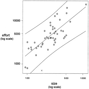
Figure 3. Data on the relationship between development effort and product size in a COBOL development organization.
A least squares fit to these data yields
|
|
Coeff. |
SE |
t |
|
Intercept |
1.120 |
0.3024 |
3.702 |
|
log10(size) |
1.049 |
0.1250 |
8.397 |
|
RMS |
0.194 |
|
|
The estimated intercept after fixing ß = 1 is 1.24; the resulting fit and a 95% prediction interval are overlaid on the data in Figure 3. This model predicts that it requires approximately 17 hours (= 101.24) to implement each unit of size.
Such models are used for prediction and tool validation. Consider an additional observation made of a product developed using a fourth-generation language and relational databases. Under the experimental development process, it took 710 hours to implement the product of size 183 (this point is denoted by X in Figure 3). The fitted model predicts that this product would have
taken approximately 3,000 hours to complete using the conventional development environment. The 95% prediction interval at X = 183 ranges from approximately 1,000 to 9,000 hours; thus, assuming that other factors are not contributing to the apparent short development cycle of this product, the use of those new fourth-generation tools has demonstrably decreased the development effort (and hence the cost).
Statistical Inadequacies in Estimating
Most cost estimation methods develop an initial relationship between the estimated size of a system (in lines of code, for instance) and the resources required to develop it. Such equations are often of the form illustrated in the above example: effort is proportional to size raised to the ß power. This initial estimate is then adjusted by a number of factors that are thought to affect the productivity of the specific project, such as the experience of the assigned staff, the available tools, the requirements for reliability, and the complexity of the interaction with the customer. Thus the estimating equation assumes the log linear form:
effort ≈ α size ß × a i a j a k a l a m ...a z ,
where the a's are the coefficients for the adjustment factors. Unfortunately, these adjustment factors are not treated as variables in a regression equation; rather, each has a set of fixed coefficients (termed "weighting factors") associated with each level of the variable. These are independently applied as if the variables were uncorrelated (an assumption known to be incorrect). These weighting schemes have been developed based on intuition about each variable's potential impact rather than on a statistical model fitting using historical data. Thus, although the relationship between effort and size is often recalibrated for different organizations, the weighting factors are not.
Exacerbating the problems with existing cost estimation models is the lack of rigorous validation of the equations. For instance, Boehm (1981) has acknowledged that his well-known COCOMO estimating model was not developed using statistical methods. Many individuals marketing cost estimation modeling tools denigrate the value of statistical approaches compared to clever intuition. To the extent that analytical methods are used in the development or validation of these models, they are often performed on data sets that contain as many predictor variables (productivity factors) as projects. Thus determination of the separate or individual contributions of the variables almost certainly depends too much on chance and can be distorted by collinear relationships. These models are rarely subjected to independent validation studies. Further, little research has been done that attempts to restrict these models to including only those productivity factors that really matter (i.e., subset selection).
Because of the lack of statistical rigor in most cost estimation models, software development organizations usually handcraft weighting schemes to fit their historical results. Thus, the specific instantiation of most cost estimation models differs across organizations. Under these conditions, cross-validation of the weighting schemes is very difficult, if not impossible. A new
approach to developing cost estimation models would be beneficial, one that invokes sound statistical principles in fitting such equations to historical data and to validating their applicability across organizations. If the instantiation of such models is found to be domain-specific, statistically valid methods should be sought for regenerating accurate models in different domains.
Process Volatility
In immature software development organizations, the processes used differ across projects because they are based on the experiences and preferences of the individuals assigned to each project, rather than on common organizational practice. Thus, in such organizations cost estimation models must attempt to predict the results of a process that varies widely across projects. In poorly run projects the signal-to-noise ratio is low, in that there is little consistent practice that can be used as the basis for dependable prediction. In such projects, neither the size nor the productivity factors provide any consistent insight into the resources required, since they are not systematically related to the processes that will be used.
The historical data collected from projects in immature software development organizations are difficult to interpret because they reflect widely divergent practices. Such data sets do not provide an adequate basis for validation, since process variation can mask underlying relationships. In fact, because the relationships among independent variables may change with variations in the process, different projects may require different values of the parameters in the cost estimation models. As organizations mature and stabilize their processes, the accuracy of the estimating models they use usually increases.
Maturity and Data Granularity
In mature organizations the software development process is well defined and is applied consistently across projects. The more carefully defined the process, the finer the granularity of the processes that can be measured. Thus, as software organizations mature, the entire basis for their cost estimation models can change. Immature organizations have data only at the level of overall project size, number of person-years required, and overall cost. With increasing organizational maturity, it becomes possible to obtain data on process details such as how many reviews must be conducted at each life cycle stage based on the size of the system, how many test cases must be run, and how many defects must be fixed based on the defect removal efficiency of each stage of the verification process. Thus, estimation in fully developed organizations can be based on a bottom-up analysis in which the historical data can be more accurate because the objects of estimation, and the effort they require, are more easily characterized.
As organizations mature, the structure of relevant cost estimation models can change. When process models are not defined in detail, models must take the form of regression equations based on variables that describe the total impact of a predictor variable on a project's
development cycle. There is little notion in these models of the detailed practices that make up the totality. In mature organizations such practices are defined and can be analyzed individually and built up into a total estimate. Normally the errors in estimating these smaller components are smaller than the corresponding error at the total project level, and it is assumed that the summary effect of aggregating these smaller errors is still smaller than the error in the estimate at the total project level.
Reliability of Model Inputs
Even if a cost estimation model is statistically sound, the data on which it is based can have low validity. Often, managers do not have sufficient knowledge of crucial variables that must be entered into a model, such as the estimated size of various individual components of a system. In such instances, processes exist for increasing the accuracy of these data. For instance, Delphi techniques can be used by software engineers who have previous experience in developing various system components. The less experience an organization has with a particular component of a system, the less reliable is the size estimate for that component. Typically, component sizes are underestimated, with ruinous effects on the resources and schedule estimated for a project. Sometimes historical "fudge factors" are applied to account for underestimation, although a more rigorous data-based approach is recommended. To aid in identifying the potential risks in a software development project, it would also be beneficial to have reliable confidence bounds for different components of the estimated size or effort.
Statistical methods can be applied to develop prior probabilities (e.g., for Bayesian estimation models) from knowledgeable software engineers and to adjust these using historical data. These methods should be used not only to suggest the confidence that can be placed in an estimate, but also to indicate the components within a system that contribute most to inaccuracies in an estimate.
As projects progress during their life cycle from specifications of requirements to design to generation of code, the information on which estimates can be based grows more reliable: there is thus greater certainty in estimating from the architectural design of a system or the detailed design of each module than in estimating from textual statements. In short, the sources from which estimates can be developed change as the project continues through its development cycle. Each succeeding level of input is a more reliable indicator of the ultimate system size than are the inputs available in earlier stages of development. Thus the overall estimate of size, resources, and schedule potentially becomes more accurate in succeeding phases of a project. Yet it is important to determine the most accurate indicators of crucial parameters such as size, effort, and schedule very early in a project, when the least reliable data are available. As such, there is a need for statistically valid ways of developing model inputs from less reliable forms of data (these inputs must reliably estimate later measures that will be more valid inputs) and of estimating how much error is introduced into an estimate based on the reliability of the inputs.
Managing to Estimates
Complicating the ability to validate cost estimation models from historical data is the fact that project managers try to manage their projects to meet received estimates for cost, effort, schedule, and other such variables. Thus, an estimate affects the subsequent process, and historical data are made artificially more accurate by management decisions and other factors that are often masked in project data. For instance, projects whose required level of effort has been underestimated often survive on large amounts of unreported overtime put in by the development staff. Moreover, many managers are quite skilled at cutting functionality from a system in order to meet a delivery date. In the worst cases, engineers short-cut their ordinary engineering processes to meet an unrealistic schedule, usually with disastrous results. Techniques for modeling systems dynamics provide one way to characterize some of the interactions that occur between an estimate and the subsequent process that is generated by the estimate (Abdel-Hamid, 1991).
The validation of cost estimation models must be conducted with an understanding of such interactions between estimates and a project manager's decisions. Some of these dynamics may be usefully described by statistical models or by techniques developed in psychological decision theory (Kahneman et al., 1982). Thus, it may be possible to develop a statistical dynamic model (e.g., a multistage linear model) that characterizes the reliability of inputs to an estimate, the estimate itself, decisions made based on the estimate, the resulting performance of the project, measures that emerge later in the project, subsequent decision making based on these later measures, and the ultimate performance of the project. Such models would be valuable in helping project managers to understand the ramifications of decisions based on an initial estimate and also on subsequent periodic updates.
ASSESSMENT AND RELIABILITY
Reliability Growth Modeling
Many reliability models of varying degrees of plausibility are available to software engineers. These models are applied at either the testing stage or the field-monitoring stage. Most of the models take as input either failure time or failure count data and fit a stochastic process model to reflect reliability growth. The differences among the models lie principally in assumptions made based on the underlying stochastic process generating the data. A brief survey of some of the well-known models and their assumptions and efficacy is given in Abdel-Ghaly et al. (1986).
Although many software reliability growth models are described in the literature, the evidence suggests that they cannot be trusted to give accurate predictions in all cases and also that it is not possible to identify a priori which model (if any) will be trustworthy in a particular
context. No doubt work will continue in refining these models and introducing "improved" ones. Although such work is of some interest, the panel does not believe that it merits extensive research by the statistical community, but thinks rather that statistical research could be directed more fruitfully to providing insight to the users of the models that currently exist.
The problem is validation of such models with respect to a particular data source, to allow users to decide which, if any, prediction scheme is producing accurate results for the actual software failure process under examination. Some work has been done on this problem (Abdel-Ghaly et al., 1986; Brocklehurst and Littlewood, 1992), using a combination of probability forecasting and sequential prediction, the so-called prequential approach developed by Dawid (1984), but this work has so far been rather informal. It would be helpful to have more procedures for assessing the accuracy of competing prediction systems that could then be used routinely by industrial software engineers without advanced statistical training.
Statistical inference in the area of reliability tends almost invariably to be of a classical frequentist kind, even though many of the models originate from a subjective Bayesian probability viewpoint. This unsatisfactory state of affairs arises from the sheer difficulty of performing the computations necessary for a proper Bayesian analysis. It seems likely that there would be profit in trying to overcome these problems, perhaps via the Gibbs sampling approach (see, e.g., Smith and Roberts, 1993).
Another fruitful avenue for research concerns the introduction of explanatory variables, so-called covariates, into software reliability growth models. Most existing models assume that no explanatory variables are available. This assumption is assuredly simplistic concerning testing for all but small systems involving short development and life cycles. For large systems(i.e., those with more than 100,000 lines of code) there are variables, other than time, that are very relevant. For example, it is typically assumed that the number of faults (found and unfound) in a system under test remains stable—i.e., that the code remains frozen—during testing. However, this is rarely the case for large systems, since aggressive delivery cycles force the final phases of development to overlap with the initial stages of system testing. Thus, the size of code and, consequently, the number of faults in a large system can vary widely during testing. If these changes in code size are not considered, the result, at best, is likely to be an increase in variability and a loss in predictive performance, and at worst, a poorly fitting model with unstable parameter estimates. Taking this logic one step further suggests the need to distinguish between new lines of code (new faults) and code coming from previous releases (old faults), and possibly the age of different parts of code. Of course, one can carry this logic to an extreme and have unwieldy models with many covariates. In practice, what is required is a compromise between the two extremes of having no covariates and having hundreds of them. This is where opportunities abound for applying state-of-the-art statistical modeling techniques. Described briefly below is a case study reported by Dalal and McIntosh (1994) dealing with reliability modeling when code is changing.
Example. Consider a new release of a large telecommunications system with approximately 7 million noncommentary source lines (NCSLs) and 400,000 lines of noncommentary new or changed source lines (NCNCSLs). For a faster delivery cycle, the source code used for system test was updated every night throughout the test period. At the end of each of 198 calendar days in the test cycle, the number of faults found, NCNCSLs, and the staff time spent on testing were collected. Figure 4 (top) portrays growth of the system as a function of staff time. The data are provided in Table 3.
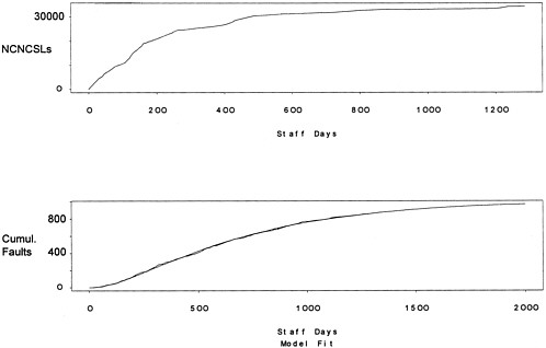
Figure 4. Plots of module size (NCNCSLs) versus staff time (days) for a large telecommunications software system (top). Observed and fitted cumulative faults versus staff time (bottom). The dotted line (barely visible) represents the fitted model, the solid line represents the observed data, and the dashed line (also difficult to see) is the extrapolation of the fitted model.
Table 3. Data on cumulative size (NCNCSLs), cumulative staff time (days), and cumulative faults for a large telecommunications system on 198 consecutive calendar days (with duplicate lines representing weekends or holidays).
|
Cum. Staff Days |
Cum. Faults |
Cum. NCNCSLs |
Cum. Staff Days |
Cum. Faults |
Cum. NCNCSLs |
Cum. Staff Days |
Cum. Faults |
Cum. NCNCSLs |
|
0 |
0 |
0 |
334.8 |
231 |
261669 |
776.5 |
612 |
318476 |
|
4.8 |
0 |
16012 |
342.7 |
243 |
262889 |
793.5 |
621 |
320125 |
|
6 |
0 |
16012 |
350.5 |
252 |
263629 |
807.2 |
636 |
321774 |
|
6 |
0 |
16012 |
356.3 |
259 |
264367 |
811.8 |
639 |
321774 |
|
14.3 |
7 |
32027 |
360.6 |
271 |
265107 |
812.5 |
639 |
321774 |
|
22.8 |
7 |
48042 |
365.7 |
277 |
265845 |
829 |
648 |
323423 |
|
32.1 |
7 |
58854 |
365.7 |
277 |
265845 |
844.4 |
658 |
325072 |
|
41.4 |
7 |
69669 |
365.7 |
277 |
265845 |
860.5 |
666 |
326179 |
|
51.2 |
11 |
80483 |
374.9 |
282 |
266585 |
876.7 |
674 |
327286 |
|
51.2 |
11 |
80483 |
386.5 |
290 |
267325 |
892 |
679 |
328393 |
|
51.2 |
11 |
80483 |
396.5 |
300 |
268607 |
895.5 |
686 |
328393 |
|
60.6 |
12 |
91295 |
408 |
310 |
269891 |
895.5 |
686 |
328393 |
|
70 |
13 |
102110 |
417.3 |
312 |
271175 |
910.8 |
690 |
329500 |
|
79.9 |
15 |
112925 |
417.3 |
312 |
271175 |
925.1 |
701 |
330608 |
|
91.3 |
20 |
120367 |
417.3 |
312 |
271175 |
938.3 |
710 |
330435 |
|
97 |
21 |
127812 |
424.9 |
321 |
272457 |
952 |
720 |
330263 |
|
97 |
21 |
127812 |
434.2 |
326 |
273741 |
965 |
729 |
330091 |
|
97 |
21 |
127812 |
442.7 |
339 |
275025 |
967.7 |
729 |
330091 |
|
97 |
21 |
127812 |
451.4 |
346 |
276556 |
968.6 |
731 |
330091 |
|
107.7 |
22 |
135257 |
456.1 |
347 |
278087 |
981.3 |
740 |
329919 |
|
119.1 |
28 |
142702 |
456.1 |
347 |
278087 |
997 |
749 |
329747 |
|
127.6 |
40 |
150147 |
456.1 |
347 |
278087 |
1013.9 |
759 |
330036 |
|
135.1 |
44 |
152806 |
460.8 |
351 |
279618 |
1030.1 |
776 |
330326 |
|
135.1 |
44 |
152806 |
466 |
356 |
281149 |
1044 |
781 |
330616 |
|
135.1 |
44 |
152806 |
472.3 |
359 |
283592 |
1047 |
782 |
330616 |
|
142.8 |
46 |
155464 |
476.4 |
362 |
286036 |
1047 |
782 |
330616 |
|
148.9 |
48 |
158123 |
480.9 |
367 |
288480 |
1059.7 |
783 |
330906 |
|
156.6 |
52 |
160781 |
480.9 |
367 |
288480 |
1072.6 |
787 |
331196 |
|
163.9 |
52 |
167704 |
480.9 |
367 |
288480 |
1085.7 |
793 |
331486 |
|
169.7 |
59 |
174626 |
486.8 |
374 |
290923 |
1098.4 |
796 |
331577 |
|
170.1 |
59 |
174626 |
495.8 |
376 |
293367 |
1112.4 |
797 |
331669 |
|
170.6 |
59 |
174626 |
505.7 |
380 |
295811 |
1113.5 |
798 |
331669 |
|
174.7 |
63 |
181548 |
516 |
392 |
298254 |
1114.1 |
798 |
331669 |
|
179.6 |
68 |
188473 |
526.2 |
399 |
300698 |
1128 |
802 |
331760 |
|
185.5 |
71 |
194626 |
527.3 |
401 |
300698 |
1139.1 |
805 |
331852 |
|
194 |
88 |
200782 |
527.3 |
401 |
300698 |
1151.4 |
811 |
331944 |
|
200.3 |
93 |
206937 |
535.8 |
405 |
303142 |
1163.2 |
823 |
332167 |
|
200.3 |
93 |
206937 |
546.3 |
415 |
304063 |
1174.3 |
827 |
332391 |
|
200.3 |
93 |
206937 |
556.1 |
425 |
305009 |
1174.3 |
827 |
332391 |
|
207.2 |
97 |
213093 |
568.1 |
440 |
305956 |
1174.3 |
827 |
332391 |
|
211.9 |
98 |
219248 |
577.2 |
457 |
306902 |
1184.6 |
832 |
332615 |
|
217 |
105 |
221355 |
578.3 |
457 |
306902 |
1198.3 |
834 |
332839 |
|
223.5 |
113 |
223462 |
578.3 |
457 |
306902 |
1210.3 |
836 |
333053 |
|
227 |
113 |
225568 |
587.2 |
467 |
307849 |
1221.1 |
839 |
333267 |
|
227 |
113 |
225568 |
595.5 |
473 |
308795 |
1230.5 |
842 |
333481 |
|
227 |
113 |
225568 |
605.6 |
480 |
309742 |
1231.6 |
842 |
333481 |
|
234.1 |
122 |
227675 |
613.9 |
491 |
310688 |
1231.6 |
842 |
333481 |
|
241.6 |
129 |
229784 |
621.6 |
496 |
311635 |
1240.9 |
844 |
333695 |
|
250.7 |
141 |
233557 |
621.6 |
496 |
311635 |
1249.5 |
845 |
333909 |
|
259.8 |
155 |
237330 |
621.6 |
496 |
311635 |
1262.2 |
849 |
335920 |
|
268.3 |
166 |
241103 |
623.4 |
496 |
311635 |
1271.3 |
851 |
337932 |
|
268.3 |
166 |
241103 |
636.3 |
502 |
311750 |
1279.8 |
854 |
339943 |
|
268.3 |
166 |
241103 |
649.7 |
517 |
311866 |
1281 |
854 |
339943 |
|
277.2 |
178 |
244879 |
663.9 |
527 |
312467 |
1281 |
854 |
339943 |
|
285.5 |
186 |
247946 |
675.1 |
540 |
313069 |
1287.4 |
855 |
341955 |
|
294.2 |
190 |
251016 |
677.4 |
543 |
313069 |
1295.1 |
859 |
341967 |
|
295.7 |
190 |
251016 |
677.9 |
544 |
313069 |
1304.8 |
860 |
341979 |
|
298 |
190 |
254086 |
688.4 |
553 |
313671 |
1305.8 |
865 |
342073 |
|
298 |
190 |
254086 |
698.1 |
561 |
314273 |
1313.3 |
867 |
342168 |
|
298 |
190 |
254086 |
710.5 |
573 |
314783 |
1314.4 |
867 |
342168 |
|
305.2 |
195 |
257155 |
720.9 |
581 |
315294 |
1314.4 |
867 |
342168 |
|
312.3 |
201 |
260225 |
731.6 |
584 |
315805 |
1320 |
867 |
342262 |
|
318.2 |
209 |
260705 |
732.7 |
585 |
315805 |
1325.3 |
867 |
342357 |
|
328.9 |
224 |
261188 |
733.6 |
585 |
315805 |
1330.6 |
870 |
342357 |
|
334.8 |
231 |
261669 |
746.7 |
586 |
316316 |
1334.2 |
870 |
342358 |
|
334.8 |
231 |
261669 |
761 |
598 |
316827 |
1336.7 |
870 |
342358 |
|
SOURCE: Dalal and McIntosh (1994). |
||||||||
Assume that the testing process is observed at time t i , i = 0 , ... , h , , and at any given time, the amount of time it takes to find a specific ''bug" is exponential with rate m . At time , the total number of faults remaining in the system is Poisson with mean l i +1, and NCNCSL is increased by an amount . This change adds a Poisson number of faults with mean proportional to C, say qC i . These assumptions lead to the mass balance equation, namely, that the expected number of faults in the system at ti (after possible modification) is the expected number of faults in the system atti -1 adjusted by the expected number found in the interval (t i -1, t i ) plus the faults introduced by the changes made at t i :
l i+1 = lie-m( ti-t i-1)+qCi,
for i =1,...h . Note that represents the number of new faults entering the system per additional NCNCSL, and represents the number of faults in the code at the start of system test. Both of these parameters make it possible to differentiate between the new code added in the current release and the older code. For the data at hand, the estimated parameters are q = 0.025 ,m = 0.002, and l 1 = 41 . The fitted and the observed data are plotted against staff time in Figure 4 (bottom). The fit is evidently very good. Of course assessing the model on independent or new data is required for proper validation.
The efficacy of creating a statistical model is now examined. The estimate of q is highly significant, both statistically and practically, showing the need for incorporating changes in NCNCSLs as a covariate. Its numerical value implies that for every additional 10,000 NCNCSLs added to the system, 25 faults are being added as well. For these data, the predicted number of faults at the end of the test period is Poisson distributed with mean 145. Dividing this quantity by the total NCNCSLs gives 4.2 per 10,000 NCNCSLs as an estimated field fault density. These estimates of the incoming and outgoing quality are very valuable in judging the efficacy of system testing and for deciding where resources should be allocated to improve the quality. Here, for example, system testing was effective in that it removed 21 of every 25 faults. However, it raises another issue: 25 faults per 10,000 NCNCSLs entering system test may be too high and a plan ought to be considered to improve the incoming quality.
None of the above conclusions could have been made without using a statistical model. These conclusions are valuable for controlling and improving the reliability testing process. Further, for this analysis it was essential to have a covariate other than time.
Influence of the Development Process on Software Dependability
As noted above, surprisingly little use has been made of explanatory variable models, such as proportional hazards regression, in the modeling of software dependability. A major reason, the panel believes, is the difficulty that software engineers have in identifying variables that can
play a genuinely explanatory role. Another difficulty is the comparative paucity of data owing to the difficulties of replication. Thus, for example, for purposes of identifying those attributes of the software development process that are drivers of the final product's dependability, it is very difficult to obtain something akin to a "random sample" of "similar" subject programs. Those issues are not unlike the ones faced in other contexts where these techniques are used, for example, in medical trials, but they seem particularly acute for evaluation of software dependability.
A further problem is that the observable in this software development application is a realization of a stochastic process, and not merely of a lifetime random variable. Thus there seems to be an opportunity for research into models that, on the one hand, capture current understanding of the nature of the growth in reliability that takes place as a result of debugging and, on the other hand, allow input about the nature of the development process or the architecture of the product.
Influence of the Operational Environment on Software Dependability
It can be misleading to talk of the reliability of a program: as is the case for the reliability of hardware, the reliability of a program depends on the nature of its use. For software, however, one does not have the simple notions of stress that are sometimes plausible in the hardware context. It is thus not possible to infer the reliability of a program in one environment from evidence of the program's failure behavior in another. This is a serious difficulty for several reasons.
First, one would like to be able to predict the operational reliability of a program from test data. The simplest approach at present is to ensure that the test environment, that is, the type of usage, is exactly similar to, or differs in known proportions for specified strata from, the operational environment. Real software testing regimes are often deliberately made to be different from operational ones, since it is claimed that in this way reliability can be achieved more efficiently: this argument is similar to that for hardware stress testing but is much less convincing in the software context.
A further reason to be interested in this problem of inferring program reliability is that most software gets broadly distributed to diverse locations and is used very differently by different users: there is great disparity in the population of user environments. Vendors would like to be able to predict different users' perceptions of a product's reliability, but it is clearly impractical to replicate in a test every different possible operational environment. Vendors would also like to be able to predict the characteristics of a population of users. Thus it might be expected that a less disparate population of users would be preferable to a more disparate one: in the former case, for example, problems reported at different sites might be similar and thus be less expensive to fix.
Explanatory variable modeling may play a useful role if suitably informative, measurable attributes of operational usage can be identified. There may be other ways of forming stochastic characterizations of operational environments. Markov models of the successive activation of modules, or of functions, have been proposed (Littlewood, 1979; Siegrist, 1988a,b) but have not
been widely used. Further work on such approaches, and on the problems of statistical inference associated with them, could be promising.
Safety-Critical Software and the Problem of Assuring Ultrahigh Dependability
It seems clear that computers will play increasingly critical roles in systems upon which human lives depend. Already, systems are being built that require extremely high dependability—a figure of 10-9 probability of failure per hour of flight has been stated as the requirement for recent fly-by-wire systems in civil aircraft. There are clear limitations to the levels of dependability that can be achieved when we are building systems of a complexity that precludes claims that they are free of design faults. More importantly, even if we were able to build a system to meet a requirement for ultrahigh dependability, we could have only low confidence that we had achieved that goal, because the problem of assessing these levels is such that it would be impractical to acquire sufficient supporting evidence (Littlewood and Strigini, 1993).
Although a complete solution to the problem of assessing ultrahigh dependability is not anticipated, there is certainly room for improving on what can be done currently. Probabilistic and statistical problems abound in this area, and it is necessary to squeeze as much as possible from relatively small amounts of often disparate evidence. The following are some of the areas that could benefit from investigation.
Design Diversity, Fault Tolerance, and General Issues of Dependence
One promising approach to the problem of achieving high dependability (here reliability and/or safety) is design diversity: building two or more versions of the required program and allowing an adjudication mechanism (e.g., a voter) to operate at run-time. Although such systems have been built and are in operation in safety-critical contexts, there is little theoretical understanding of their behavior in operation. In particular, the reliability and safety models are quite poor.
For example, there is ample evidence (Knight and Leveson, 1986) that, in the presence of design faults, one cannot simply assume that different versions will fail independently of one another. Thus the simple hardware reliability models that involve mere redundancy, and assume independence of component failures, cannot be used. It is only quite recently that probability modeling has started to address this problem seriously (Eckhardt and Lee, 1985; Littlewood and Miller, 1989). These models provide a formal conceptual framework within which it is possible to reason about the subtle issues of conditional independence involved in the failure processes of design-diverse systems. However, they provide little quantitative practical assistance to a software designer or evaluator.
Further probabilistic modeling is needed to elucidate some of the complex issues. For example, little attention has been paid to modeling the full fault tolerant system, involving diversity and adjudication. In particular, the properties of the stochastic process of failures of
such systems are not understood. If, as seems likely, individual versions of a program in a real-time control system exhibit clusters of failures in time, how does the cluster process of the system relate to the cluster processes of the individual versions? Although such issues seem narrowly technical, they are vitally important in the design of real systems, whose physical integrity may be sufficient to survive one or two failed input cycles, but not many.
Another area that has had little work is probabilistic modeling of different possible adjudication mechanisms and their failure processes.
Judgment and Decision-making Framework
Although probability seems to be the most appropriate mechanism for representing uncertainty about system dependability, other candidates such as Shafer-Dempster and possibility theories might be plausible alternatives in safety-critical contexts where quantitative measures are required in the absence of data—for example, when one is forced to rely on the engineering judgment of an expert. Further work is needed to elucidate the relative advantages and disadvantages of the different approaches applicable in the software engineering domain.
There is evidence that human judgment, even in "hard" sciences such as physics, can be seriously in error (Henrion and Fischhoff, 1986): people seem to make consistent errors and tend to be optimistic in their own judgment regarding their likely error. It is likely that software engineering judgments are similarly fallible, and so this area calls for some statistical experimentation. In addition, it would be beneficial to have formal mechanisms for assessing whether judgments are well calibrated and for recalibrating judgment and prediction schemes (of humans or models) that have been shown to be inaccurate. This problem has some similarity to the problems of validating software reliability models, already mentioned, in which prequential likelihood plays a vital role. It also bears on more general applications of Bayesian modeling where elicitation of a priori probability values is required.
It seems inevitable that reasoning and judgment about the fitness of safety-critical systems will depend on evidence that is disparate in nature. Such evidence could include data on failures, as in reliability growth models; human expert judgment; results regarding the efficacy of development processes; information about the architecture of a system; or evidence from formal verification. If the required judgment depends on a numerical assessment of a system's dependability, there are clearly important issues concerning the composition of very different kinds of evidence from different sources. These issues may, indeed, be overriding when it comes to choosing among the different ways of representing uncertainty. The Bayes theorem, for example, may provide an easier way than does possibility theory to combine information from different sources of uncertainty.
A particularly important problem concerns the way in which deterministic reasoning can be incorporated into the final assessment of a system. Formal methods of achieving dependability are becoming increasingly important. Such methods range from formal notations, which assist in the elicitation and expression of requirements, to full mathematical verification of the correspondence between a formal specification and an implementation. One view is that these approaches incorporating deterministic reasoning to system development remove a particular
type of uncertainty, leaving others untouched (uncertainty about the completeness of a formal specification, the possibility of incorrect proof, and so on). One should factor into the final assessment of a system's dependability the contribution from such deterministic, logical evidence, nevertheless keeping in mind that there is an irreducible uncertainty in one's possible knowledge of the failure behavior of a system.
Structural Modeling Issues
Concerns about the safety and reliability of software-based systems necessarily arise from their inherent complexity and novelty. Systems now being built are so complex that they cannot be guaranteed to be free from design faults. The extent to which confidence can be carried over from the building of previous systems is much more limited in software engineering than in "real" engineering, because software-based systems tend to be characterized by a great deal of novelty.
Designers need help in making decisions throughout the design process, especially at the very highest level. Real systems are often difficult to assess because of early decisions regarding how much system control will depend on computers, hardware, and humans. For the Airbus A320, for example, the early decision to place a high level of trust in the computerized fly-by-wire system meant that this system (and thus its software) needed to have a better than probability of failure in a typical flight. Stochastic modeling might aid in such high-level design decisions so that designers can make "what if" calculations at an early stage.
Experimentation, Data Collection, and General Statistical Techniques
A dearth of data has been a problem in much of safety-critical software engineering since its inception. Only a handful of published data sets exists even for the software reliability growth problem, which is by far the most extensively developed aspect of software dependability assessment. When the lack of data arises from the need for confidentiality—industrial companies are often reluctant to allow access to data on software failures because of the possibility that people may think less highly of their products—little can be done beyond making efforts to resolve confidentiality problems. However, in some cases the available data are sparse because there is no statistical expertise on hand to advise on ways in which data can be collected cost-effectively. It may be worthwhile to attempt to produce general guidelines for data collection that address the specific difficulties of the software engineering problem domain.
With notable exceptions (Eckhardt et al., 1991; Knight and Leveson, 1986), experimentation has so far played a low-key role in software engineering research. Somewhat surprisingly, in view of its difficulty and cost, the most extensive experimentation has investigated the efficacy of design diversity. Other areas where experimental approaches seem feasible and should be encouraged include the obvious and general question of which software development methods are most cost-effective in producing software products with desirable attributes such as dependability. Statistical advice on the design of such experiments would be essential; it might
also be the case that innovation in the design of experiments could make feasible some investigations that currently seem too expensive to contemplate: the main problem arises from the need for replication over many software products.
On the other hand, areas where experiments can be conducted without the replication problem being overwhelming involve the investigation of quite restricted hypotheses about the effectiveness of specific techniques. For example, experimentation could address whether the techniques that are claimed to be effective for achieving reliability (i.e., effectiveness of debugging) are significantly better than those, such as operational testing, that will allow reliability to be measured.
SOFTWARE MEASUREMENT AND METRICS
Measurement is at the foundation of science and engineering. An important goal shared by software engineers and statisticians is to derive reliable, reproducible, and accurate measures of software products and processes. Measurements are important for assessing the effects of proposed "improvements" in software production, whether they be technological or process oriented. Measurements serve an equally important role in scheduling, planning, resource allocation, and cost estimation (see the first section in this chapter).
Early pioneering work by McCabe (1976) and Halstead (1977) seeded the field of software metrics; an overview is provided by Zuse (1991). Much of the attention in this area has focused on static measurements of code. Less attention has been paid to dynamic measurements of software (e.g., measuring the connectivity of software modules under operating conditions) and aspects of the software production process such as software reuse, especially in systems employing object-oriented languages.
The most widely used code metric, the NCSL (noncommentary source line), is often used as a surrogate for functionality. Surprisingly, since software is now nearly 50 years old, standards for counting NCSLs remain elusive in practice. For example, should a single, two-line statement in C language count as one NCSL or two?
Counts of tokens (operators or operands), delimiters, and branching statements are used as other static metrics. Although some of these are clearly measures of software size, others purport to measure more subtle notions of software complexity and structure. It has been observed that all such metrics are highly correlated with size. At the panel's information-gathering forum, Munson (1993) concluded that current software metrics capture approximately three "independent" features of a software module: program control, program size, and data structure. A statistical (principal-components) analysis of 13 metrics on HAL programs in the space shuttle program was the key to this finding. While one might argue that performing a common statistical decomposition of multivariate data is hardly novel, it most certainly is in software engineering. The important implication of that finding is that there are features of software that are not being captured by the existing battery of software metrics (e.g., cohesion and coupling)—and if these are key differentiators of potentially high- and low-fault programs, there is no way that an analysis of the available metrics will highlight this condition. On the other side of the ledger, the statistical costs of including "noisy" versions of the same (latent) variable in models and analysis
methods that are based on these metrics, such as cost estimation, seem not to have been appreciated. Subset selection methods (e.g., Mallows, 1973) provide one way to assess variable redundancy and the effect on fitted models, but other approaches that use judgment composites, or composites based on other bodies of data (Tukey, 1991), will often be more effective than discarding metrics.
Metrics typically involve processes or products, are subjective or objective, and involve different types of measurement scales, for example, nominal, ordinal, interval, or ratio. An objective metric is a measurement taken on a product or process, usually on an interval or ratio scale. Some examples include the number of lines of code, development time, number of software faults, or number of changes. A subjective metric may involve a classification or qualification based on experience. Examples include the quality of use of a method or the experience of the programmers in the application or process.
One standard for software measurement is the Basili and Weiss (1984) Goal/Question/ Metric paradigm, which has five parameters:
-
An object of the study—a process, product, or any other experience model;
-
A focus—what information is of interest;
-
A point of view—the perspective of the person needing the information;
-
A purpose—how the information will be used; and
-
A determination of what measurements will provide the information that is needed.
The results are studied relative to a particular environment.


