
3
Statistics and Data Analysis
The National Highway Traffic Safety Administration’s (NHTSA’s) final rule regarding consumer information on rollover resistance (Federal Register 2001) notes that “the effect of SSF [static stability factor] must be shown to have a significant influence on the outcome of actual crashes (rollover vs. no rollover) to be worth using for consumer information.” To this end, the agency undertook a statistical study to investigate the relationship between measured values of SSF for a range of vehicles and corresponding rollover rates determined from real-world crash data (Federal Register 2000). The agency subsequently conducted further statistical analyses in response to public comment on the first study (Federal Register 2001).
As noted in Chapter 1, rollover crashes are complex events influenced by driver characteristics, the driving environment, and the vehicle and the interaction among the three. Therefore, one of the challenges in analyzing rollover crash data is to isolate the effect of a particular variable—such as SSF—from that of other variables. Differences in rollover risk1 due to how, when, where, and by whom a vehicle is operated complicate comparisons of the rollover risk of different vehicles. NHTSA’s analyses of crash data involved the use of binary-response models. A binary-response model is a regression model in which the dependent variable (outcome of the crash) is binary (“rollover” or “no rollover”). NHTSA used such models to study the effect of various explanatory variables—such as driver characteristics, environmental conditions, and vehicle metrics—on the probability of rollover.
According to NHTSA, the results of its statistical analyses reveal that, in the event of a single-vehicle crash, the effect2 of SSF on the probability of rollover is highly important, even when driver characteristics—such as age—and environmental characteristics—such as road and weather conditions—contribute to the crash. This statistical correlation between SSF and the probability of rollover is the foundation for NHTSA’s star rating system for rollover resistance and for the one- to five-star ratings assigned to different vehicles.
This chapter presents the committee’s review of the statistical analyses that form the basis for NHTSA’s rollover resistance rating system. The results of additional statistical analyses performed by the agency at the committee’s request are also discussed. The purpose of all these analyses was to investigate what crash data indicate about the effect of SSF on a vehicle’s propensity to roll over. The chapter begins with a review of the available sources of crash data and a description of the data selected by NHTSA for use in its analyses. Some basic statistical ideas and the notation used in the chapter are then presented. The next section describes the binary-response models used by NHTSA in constructing a rating system. The influence of the driver and driving environment on the probability of rollover is then examined in depth, and a preliminary estimate of a nonparametric version of the binary-response model for rollovers is presented. Next, the potential—from a statistical perspective—of the binary-response models used by NHTSA to provide practical, useful information to the public is examined. The chapter concludes with a summary of the committee’s findings and recommendations in the area of statistics and data analysis.
ROLLOVER CRASH DATA
This section begins with a brief overview of the major sources of data available to NHTSA for the purposes of its statistical analysis of rollover crashes. The rationale behind the agency’s choice of crash data is then reviewed, with particular emphasis on the selection of data from six states for use in constructing the rollover resistance rating system.
Crash Data Files
Four major databases maintained by NHTSA have the potential to support evaluation of rollover collisions, including rollover rates:
-
State Data System (SDS);
-
Fatality Analysis Reporting System (FARS);
-
General Estimates System (GES); and
-
Crashworthiness Data System (CDS).
Table 3-1 summarizes the key features of these databases. All four include some information on rollover crashes. As indicated in the table, however, there are variations in the numbers of rollovers reported and in the level of detail provided about each crash (e.g., extent of injuries or information on crash site).
TABLE 3-1 Features of NHTSA’s Major Crash Databases
|
Database |
Key Features |
Data on Rollover Crashes |
|
State Data System (SDS) |
|
|
|
Fatality Analysis Reporting System (FARS) |
|
|
|
General Estimates System (GES) |
|
|
|
Crashworthiness Data System (CDS) |
|
|
Rationale Behind NHTSA’s Selection of Data
The crash data used by NHTSA to develop statistical models are derived from police crash reports and form part of the SDS. The decision to use data from specific states within the SDS was driven largely by the desire to have a robust data set for the analysis. The GES and CDS were judged inappropriate because the numbers of rollover crashes reported in these databases are relatively small. And although the FARS database includes a moderate number of rollovers, the restriction to fatal crashes limits the range of crash scenarios represented in which a vehicle may overturn.
Although the police-reported data in the SDS are the most important in understanding NHTSA’s modeling efforts, the three other databases man-
aged by NHTSA and listed in Table 3-1 are often referenced in reports and documents addressing the rollover crash problem.
All three of these databases were considered by NHTSA in the process of identifying appropriate data for statistical modeling. Thus although the FARS, GES, and CDS databases were deemed inadequate, they were useful in informing NHTSA’s analyses.
Importance of Single-Vehicle Crashes
NHTSA’s analyses used SDS crash data relating to single-vehicle events only (see below). Indeed, although FARS and GES data were not used to derive the statistical correlation between rollover rates and SSF, these data highlight the preponderance of rollover-related deaths and injuries associated with single-vehicle crashes. For example:
-
Analysis of 1999 FARS data shows that 82 percent of light-vehicle rollover fatalities were associated with single-vehicle crashes.
-
According to 1999 FARS data, rollover accounted for 55 percent of all occupant fatalities for single-vehicle crashes involving light vehicles.
-
GES data for the period 1995–1999 indicate that, on average, 241,000 light vehicles rolled over each year nationwide. Of this total, 205,000 (85 percent) were single-vehicle events that resulted in 46,000 severe (incapacitating) or fatal injuries.
Tripped Versus Untripped Rollover
The CDS database—part of the National Automotive Sampling System (NASS)—identifies many different categories of rollover, including “tripover” (also known as tripped rollover) and “turn-over” (also known as untripped rollover).3 The different rollover types coded in the CDS database are determined primarily from crash scene and vehicle inspections, with additional evidence derived from photographs, police reports, and interviews with drivers and others.4 It is widely acknowledged that the interpretation of crash scene evidence can be problematic, with resulting uncertainties in distinguishing between tripped and untripped rollovers. In 1998, the coding of a number of crashes in the CDS database for the period 1992–1996 was revisited, and revisions were made. In particular, many of crashes originally coded as untripped were recoded as tripped (NHTSA 1999). NHTSA has sought to demonstrate that the vast majority of single-vehicle passenger-vehicle rollovers
|
3 |
See Chapter 2 for definitions of tripped and untripped rollover. |
|
4 |
“Collection of NASS CDS Data Relating to Rollover,” presentation to the Committee for the Study of a Motor Vehicle Rollover Rating System by Robert Woodill (Veridian Engineering) and John Brophy (NHTSA), Washington, D.C., May 29, 2001. |
are tripped. According to the agency’s analysis of CDS data for the period 1992 through 1996, more than 95 percent of single-vehicle crashes involving rollover were tripped (NHTSA 1999; Federal Register 2001).
As noted in Chapter 2, it is the magnitude and duration of the forces on a vehicle—rather than the tripping mechanism—that determine whether rollover occurs. In light of this observation, as well as the practical difficulties involved in distinguishing the two categories of rollover, tripped and untripped rollovers are not addressed separately in the present discussion. Moreover, the SDS data used by NHTSA in developing its rollover probability model and subsequent rating system do not distinguish between the two types of rollovers, and crash data for both types were included in the agency’s statistical analyses.
State Selection
NHTSA’s analyses were based on SDS data for specific states, selected on the basis of the following criteria (Federal Register 2000):
-
The state had to participate in the SDS and must have provided data for 1997.5
-
The vehicle identification number (VIN) had to be included in the electronic file.
-
The file had to include a variable indicating whether a rollover occurred as either the first or a subsequent event in the crash.
NHTSA selected six states for modeling: Florida, Maryland, Missouri, North Carolina, Pennsylvania, and Utah. The corresponding single-vehicle crash data were used in the modeling analysis that resulted in the curve used to establish the star rating values for individual vehicle models. Data from New Mexico and Ohio were also used for some of the supporting analyses, but were not included in the modeling efforts because of differences in crash reporting practices.
Single-vehicle crashes served as the exposure measure for assessing the relative magnitude of the rollover problem (i.e., number of rollover events or number of single-vehicle crashes). The crashes included in the analysis were single-vehicle collisions for all light vehicles (less than 10,000 pounds gross vehicle weight) between 1994 and 1998 (see Table 3-2). Such crashes were defined as not involving another motor vehicle, pedestrian, bicyclist, animal, or train. Special classes of vehicles were also excluded from the analysis, notably emergency vehicles (e.g., fire, ambulance, police, or military), parked vehicles, and vehicles pulling a trailer. The total number of single-vehicle crashes initially included in the dataset was 227,194.
TABLE 3-2 Single-Vehicle Crash Frequencies for Six States Included in Modeling Analysis
NHTSA identified 100 different vehicle make and model combinations, each with a unique SSF (see Federal Register 2001, Appendix I). All the 227,194 single-vehicle crashes in the dataset involved vehicles with VINs that matched one of the 100 groups. However, any of the 100 make and model groups for which there were fewer than 25 crashes were excluded from the analysis. The final dataset used for analysis comprised 226,117 crashes in 87 make and model groups. Of these crashes, 45,574 (20.16 percent) resulted in rollover.
In light of NHTSA’s responsibilities for establishing national policy and providing information relevant at the national level, it is important that the rollover crash data used to derive consumer information be representative of all states. Hence, the agency undertook an additional effort that involved using the GES database to determine whether the rollover rate for a national sample of single-vehicle crashes was similar to the rate for the six states included in the original analysis. Using GES data for 1994 through 1998 (the same years as the SDS data), a total of 9,910 vehicles were identified that (1) had VINs that placed them in the group of 100 make/model categories, and (2) were involved in single-vehicle crashes. Of these vehicles, 2,377 rolled over. After applying the appropriate weighting factors to account for the GES sampling scheme, NHTSA obtained national estimates for single-vehicle crashes and subsequent rollover crashes of 1,185,474 and 236,335, respectively. The resulting rollover rate was 19.94 percent—essentially the same as the rate of 20.16 percent derived for the six states used in the modeling analysis.
BACKGROUND AND NOTATION
This section reviews some basic statistical ideas relevant to the present discussion, together with the notation used in statistical analyses of rollover crash data. As stated earlier, NHTSA’s rollover resistance rating system is
based on a binary-response model of rollover events. The dependent variable and explanatory variables of the model are first described, and the specification of the relation between the dependent variable and explanatory variables is then discussed. Finally, the concept of the rollover curve—the basis for NHTSA’s rating system—is introduced, and two interpretations of this curve are presented.
Dependent and Explanatory Variables
The binary-response model for rollovers states that the probability of rollover, given that a single-vehicle crash has occurred, is a certain function of selected explanatory variables. Let Y denote the dependent variable in a binary-response model of rollovers. This variable Y is equal to 1 if there is a rollover and 0 otherwise. Thus, the probability of a rollover is the probability that Y = 1. This probability depends on the values of the explanatory variables incorporated in the model.
The commonly used explanatory variables include driver characteristics, environmental variables, and vehicle metrics. An example of a driver variable is YOUNG (Z1), where Z1 = 1 if the driver is under 25 years old and 0 otherwise. An example of a road condition variable is CURVE (Z2), where Z2 = 1 if the crash occurred on a curve area and 0 otherwise. An example of a vehicle metric is SSF, which is denoted by X.
The explanatory variables are typically divided into two groups: the vehicle metrics are in one group and the driver characteristics and environmental variables in the other. This latter group defines what is called a scenario. Let Z denote the array of driver and environmental variables. To simplify the exposition, suppose a scenario is defined by one driver variable and one environmental variable, unless noted otherwise. In this case, Z has only two components: Z = (Z1, Z2). If a scenario is defined by the variables YOUNG and CURVE, there are four possible scenarios: (0,0), (0, 1), (1,0), (1,1). For example, the scenario (1,1) describes the case of a single-vehicle accident involving a young driver on a curve.
SSF is the only vehicle metric used by NHTSA for the purpose of constructing a rating system. However, because driver and environmental variables also may be important in determining rollover risk, variables in these other categories were considered as well. These variables are explained in Table 3-3. The criterion for the selection of the driver and environmental variables was the availability of appropriate data both within the GES and for the six SDS states used in NHTSA’s analysis. The variables ultimately considered in the models were DARK, STORM, FAST, HILL, CURVE, BADSURF, MALE, YOUNG, OLD, and DRINK (see Table 3-3).
NHTSA also included the six SDS states as explanatory variables. An example of a state variable is S1, say, where S1 = 1 if Florida is the state in which the single-vehicle crash occurred and 0 otherwise. The need for these state-
TABLE 3-3 Variables Available for Inclusion in NHTSA’s SSF-Rollover Rate Model
|
Variable |
Definition |
|
ROLLa |
Proportion of single-vehicle crashes that involved a rollover |
|
SSFa |
Numeric value of static stability factor |
|
DARKa |
Proportion of single-vehicle crashes that occurred during darkness |
|
STORMb |
Proportion of single-vehicle crashes that occurred during inclement weather |
|
RURAL |
Proportion of single-vehicle crashes that occurred in rural areas |
|
FASTb |
Proportion of single-vehicle crashes that occurred on roadways where the speed limit was 50 mph or greater |
|
HILLb |
Proportion of single-vehicle crashes that occurred on a grade, at a summit, or at a dip |
|
CURVEb |
Proportion of single-vehicle crashes that occurred on a curve |
|
BADROAD |
Proportion of single-vehicle crashes that occurred on roads with potholes or other bad road conditions |
|
BADSURFa |
Proportion of single-vehicle crashes that occurred on wet, icy, or other bad surface conditions |
|
MALEb |
Proportion of single-vehicle crashes involving a male driver |
|
YOUNGb |
Proportion of single-vehicle crashes involving a driver under 25 years old |
|
OLDb |
Proportion of single-vehicle crashes involving a driver age 70 or older |
|
NOINSURE |
Proportion of single-vehicle crashes involving an uninsured driver |
|
DRINKb |
Proportion of single-vehicle crashes involving a driver who was drinking or using illegal drugs |
|
NUMOCC |
Average number of vehicle occupants |
|
a Variable included in models. b Environmental or driver variable found statistically significant in models. SOURCES: Federal Register 2000, 2001 (Table 7). |
|
based variables is explained by the known differences among states in crash reporting practices (see Federal Register 2001, Table 5), roadway characteristics, driver demographics and vehicle usage patterns, and other such factors.
As discussed in Chapter 2, physics indicates that SSF is an indicator of a vehicle’s rollover propensity. The purpose of the statistical analysis is to investigate what the crash data indicate about the effect of SSF on a vehicle’s propensity to roll over and whether the magnitude of this effect depends on driver and environmental variables. The example of a double-decker bus illustrates the complexities involved in interpreting the results of such crash data analyses. The double-decker bus has a low SSF. This fact does not automatically imply that accident data for the double-decker bus will show that SSF is strongly correlated with the incidence of rollover, because the accident history depends on the bus driver and the driving conditions as well as on SSF. If a double-decker bus is normally driven by a professional driver in an urban area, the number of accidents is likely to be low, and in the accidents that do occur, there are likely to be relatively few rollovers. This example illustrates that the scenario can attenuate the observed effect of SSF. At the same time, however, the accident history in this example does not negate the fundamental physics of rollover. Thus SSF remains important in determining a vehicle’s
rollover propensity, as discussed in Chapter 2, although its influence is not clearly manifested in the crash data because the double-decker bus is rarely involved in higher-risk scenarios, and these vehicles experience relatively few rollovers.
Functional Forms
The statistical problem is to estimate the probability that Y = 1 (i.e., the probability of a rollover), considered as a function of the explanatory variables. For this purpose, the conventional approach is to specify what is called a parametric binary-response model. In this approach, the form of the relation between the probability that Y = 1 and the explanatory variables is assumed known, while the values of certain parameters in the relationship are to be determined. Linear regression analysis is a well-known example of this approach. In linear regression analysis, the relation between the dependent and explanatory variables is assumed to be linear, but the values of the coefficients in the linear relation are assumed to be unknown. In the case of a binary-response model, the relation between the probability that Y = 1 and the explanatory variables is generally assumed to be nonlinear.
Following the parametric approach, suppose that the true probability that Y = 1 given that Z = z and X = x is
(1)
where the function F specifies the relation between the probability that Y = 1 and the explanatory variables. The assumption is that the functional form F is known and that the values of the parameters α0, α1, α2, and β are unknown. The typical assumption is that F is a cumulative distribution function. The commonly used distribution functions are smooth S-shaped curves.
The most widely used binary-response models are logit and probit models. A binary-response model is referred to as a logit model if F is the cumulative logistic distribution function and as a probit model if F is the cumulative normal distribution function. NHTSA employed a logit model in its statistical analysis of rollover crash data. Generally, both types of models produce highly similar statistical results because the logistic and normal distributions are both symmetrical around zero and have very similar shapes, except that the logistic distribution has fatter tails.
The problem is to estimate the unknown parameters. The parameters of logit and probit models are typically estimated by maximum likelihood, and this is the estimation method used by NHTSA for its logit model. The maximum-likelihood estimator has good properties in large samples.6 In par-
ticular, it is asymptotically efficient; that is, it is the precise estimator in large samples.
Rollover Curve and Interpretations
The rating system proposed by NHTSA is based on SSF. Suppose that the (true) probability that Y = 1 given that X = x is
(2)
where the functional form G is known, and the parameters β0 and β1 are unknown. This model gives the relation between the probability that Y = 1 and X. This relation is called the rollover curve. The physics of rollover strongly suggests that the rollover curve is downward sloping; that is, the probability that Y = 1 decreases as SSF increases.
The rollover curve has two interpretations, depending on how the model G(β0 +β1x) is derived. In one interpretation, the rollover curve gives the average of the rollover probability for each value of SSF, where the average is taken over the scenarios. In this case, the rollover curve can be estimated using data on only one explanatory variable, namely SSF. In the other interpretation, the rollover curve gives the rollover probability for the average scenario. In this case, data on driver and environmental variables, as well as SSF, are used in estimating the curve. Either approach can be used to estimate the rollover curve, although the two approaches yield different results (see Box 3-1). NHTSA has employed the second approach extensively in estimating the rollover curve. This is a reasonable choice provided the average scenario is an empirically relevant baseline for comparing vehicles.
STATISTICAL MODELS
NHTSA’s initial analysis of single-vehicle crash data was based on an exponential model—a type of model that is little used in the statistical literature. The current rating system for rollover resistance was constructed using an estimated rollover curve also based on an exponential model. The uncertainties associated with this estimated rollover curve were not considered in deriving the star rating categories. Subsequently, NHTSA conducted further analyses using a logit model, which, as noted earlier, is a widely used type of binary-response model. The results obtained using the logit model are presented below.
Following a brief discussion of issues related to uncertainty in estimating statistical models, this section describes exponential and logit parametric binary-response models. The rollover curves and associated confidence intervals obtained by NHTSA in its analyses are then considered.
|
BOX 3-1 Two Interpretations of the Rollover Curve Taking the average of the rollover probability for each value of SSF, where the average is taken over the scenarios, the average rollover probability is In contrast, the rollover probability for the average scenario is where The first formula can be written as which says that P(Y = 1|X = x) is a weighted average of functions. The weighted average P(Y = 1|X = x) = G(β0 +β1x) can be estimated using data on only one explanatory variable, namely SSF. The second formula can be expressed as which says that P*(Y = 1|X = x) is a function of the average scenario. In this case, F(α0 +α1z1 +α2z2 +βx) has to be estimated to estimate P*(Y = 1|X = x); that is, the data on driver and environmental variables are also used in the estimation. The reason P(Y = 1|X = x) ≠ P*(Y = 1|X = x) is that the average of the function is not the function of the average when the function is nonlinear. NHTSA has employed the second formula extensively in estimating the rollover curve. |
Confidence Intervals
In reporting the results of estimation, it is good statistical practice to include some information on the reliability of the estimator—that is, the extent to which the estimate varies from sample to sample. The confidence interval for a parameter is a well-known statistical tool for evaluating the reliability of an estimator of a parameter. The parameters of interest here are the rollover probabilities in single-vehicle crashes. The width of the confidence interval associated with an estimated rollover probability reflects the uncertainty about the true value of the probability; a longer confidence interval indicates greater uncertainty. The larger the sample of crash data used in the estimation, the narrower is the width of the confidence interval for the true rollover probability, all other things being equal. Hence, a more reliable estimate of the model—and of the rollover curve—is expected from a large than from a small sample.
In the present case, NHTSA’s dataset comprising more than 226,000 single-vehicle crashes constitutes a large sample, suggesting that the confidence intervals for the rollover probabilities derived are very narrow. This suggestion is confirmed when the data are analyzed using a logit model. Specifically, statistically reliable estimates of the rollover probabilities are obtained when the logit model is estimated by maximum likelihood from the ungrouped binary data. Consequently, statistical uncertainty about the rollover curve is not an issue when the logit model is used. However, NHTSA initially estimated a version of the exponential model using grouped data (make and model data). The associated confidence intervals were computed using formulas appropriate for the standard normal linear model and are relatively wide. The rollover probabilities can be estimated reliably provided the appropriate statistical methodology is used. The following discussion provides further insights into the issue of model choice.
Exponential Model
The exponential model is as follows:
(3)
Taking the logarithm of both sides, this model can be written as
(4)
NHTSA refers to this model as a linear model. In principle, Formulation 3 can be estimated directly from binary data. In contrast, Linear Model 4 is estimated from grouped data. The exponential model, in either its original formulation or its logarithmic version, is seldom used for analyzing binary data.
NHTSA estimated a version of the linear model using grouped data. Using these data, the unknown probability P is replaced by a sample proportion, p. This replacement yields the model
(5)
where ∈ is an error term that is approximately normally distributed. The model based on grouped data can be estimated by ordinary least squares. A better (more efficient) estimation method is to use weighted least squares because the variance of the sample proportion is not the same for all values of SSF.
NHSTA estimated a linear model that included SSF and the six state dummy variables as explanatory variables. The grouped data used to estimate the linear model were obtained as follows. The crash data were grouped into 100 make and model groups. As noted earlier, only 87 groups were used in the analysis because groups with fewer than 25 crashes were excluded (Federal Register 2001). All vehicles in a make or model group have the same SSF. The make and model groups were then sorted by state, producing 542 state and model groups. Again some groups were excluded because of the small number of crashes involved. NHTSA’s estimation was based on 518 state make and model groups, that is, a sample of 518 observations. The proportion of rollovers was computed for each state make and model group.
At the request of the Alliance of Automobile Manufacturers, Exponent Failure Analysis Associates reviewed NHTSA’s statistical analyses of crash data that serve as the basis for the star rating system for rollover resistance. As part of this review, Exponent (Donelson and Ray 2001) calculated confidence intervals for the rollover probabilities using formulas that are appropriate in the case of the standard linear normal regression model. NHTSA redid these calculations and obtained essentially the same results as Exponent. Figure 3-1 shows the estimated rollover curve and the 95 percent confidence intervals obtained by NHTSA.
The confidence intervals in Figure 3-1 are wide when SSF is low and become progressively narrower as SSF increases in value. Thus, for a sport utility vehicle (SUV) with an SSF of 1.1, the rollover probability in the event of a single-vehicle crash is approximately 0.26–0.42; this vehicle would receive a rollover resistance rating of one to three stars. In contrast, a passenger car with an SSF of 1.4 has a rollover probability of approximately 0.10–0.17 and would be assigned a four-star rating. What this analysis appears to show is that the uncertainty associated with the estimates is too large to permit accurate discrimination among SUVs. If this analysis is correct, a rating system based on a linear model does not provide information that can be used to distinguish among the rollover propensities of different SUVs.
NHTSA also calculated the confidence intervals using data that had been adjusted for national average road use and for differences in reporting practices. The resulting intervals are narrower because the adjustments smooth
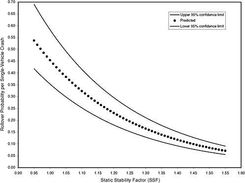
FIGURE 3-1 Estimate of probability of rollover and 95 percent confidence intervals for exponential model.
the grouped data; that is, they reduce the scatter of the sample proportions about the estimated rollover curve.
The confidence intervals reported in Figure 3-1 are based on a flawed statistical analysis. The flaw is that the confidence intervals calculated by Exponent and NHTSA depend only on the number of make and model groups, ignoring the states. For purposes of illustration, assume there are 100 make and model groups. If the number of crashes in the crash dataset is doubled, there are still 100 make and model groups. Thus, the confidence intervals do not shrink as expected with an increase in the number of crashes in the dataset. Hence, an increase in the size of the crash dataset does not improve the accuracy of the estimates according to the formulas employed by Exponent and NHTSA. This result indicates that something is wrong with the method used to calculate the confidence intervals shown in Figure 3-1.
Technically speaking, the widths of the confidence intervals depend on the estimated variances and covariances of the estimates of the parameters of the linear model. In the formulas used by Exponent and NHTSA, the estimated variances and covariances depend only on the number of make and model groups, not on the number of crashes in the dataset.
The make and model data have engendered confusion about the role of the rollover curve. If the objective is to estimate the true probability of rollover
for a given make or model group, then the best estimate of the rollover probability is obtained from the history of crashes for that group. In particular, the best estimate is the sample proportion of rollovers calculated from the crash data for that make or model. This is to say that the sample mean is the best estimate of the population mean. The implicit assumption is that a crash dataset is available for a given make or model—there is a history. Hence, if the objective is to estimate the make or model rollover probability for an old make or model group, there is no reason to estimate the rollover curve.
For new make and model groups there is no crash history, or a very limited one; that is, the crash dataset contains a small number of crashes, if any. The problem then arises of how to predict the rollover probability for these make and model groups. The rollover curve provides a solution, assuming that the relation between the rollover probability and SSF is the same for new as for old makes and models. What is known about the new make or model is its SSF. Given the SSF of the new make or model, the estimated rollover curve can be used to predict the rollover probability.
Logit Model
The logit model is as follows:
(6)
Taking the logarithm of both sides, this model can be written as
(7)
where P/(1 − P) is called the odds ratio. The first formulation of Model 6 can be estimated from binary data by maximum likelihood. The software for maximum-likelihood estimation of Model 6 is widely available. The logarithmic version can be estimated by using grouped data.
A comparison of the logarithmic versions of the exponential and logit models shows that if the functional form of the logit model is correct, the functional form of the exponential model is misspecified. The logit and exponential functional forms cannot both be correct simultaneously.
There are two approaches for obtaining tight confidence intervals for the rollover probabilities. One is to estimate the exponential model by maximum likelihood using the ungrouped binary data. A more attractive approach is to switch to the logit model. As a practical matter, maximum-likelihood estimation of the logit model with ungrouped data can easily be implemented with available off-the-shelf statistical software. From a theoretical point of view, the logit model has more desirable properties than the exponential model. For example, an important property of the logit model is that it constrains true probabilities to lie between 0 and 1, and similarly for the prob-
abilities estimated by maximum likelihood. The same is not the case for the exponential model. The confidence intervals for the rollover curve based on the logit model are presented below.
The committee asked NHTSA to calculate the large-sample 95 percent confidence intervals for rollover probabilities based on maximum-likelihood estimation of the logit model using ungrouped binary data. The logit model included as explanatory variables SSF, driver and environmental variables, scenario dummy variables, and five state dummy variables (Missouri, the sixth state, was used as the baseline). The formula for the large-sample confidence interval is available in the statistical literature (see, for example, Greene 2000, p. 824). The estimated rollover curve and the 95 percent confidence intervals using the data for the six states combined are shown in Figure 3-2.7 The maximum-likelihood estimates of the parameters of the logit model are reported in Appendix C.8
The first point to note is that an increase in SSF reduces the probability of rollover. The second point is that the widths of the confidence intervals

FIGURE 3-2 Estimated probability of rollover and 95 percent confidence intervals based on maximum-likelihood estimation of a logit model using data from six states combined (n = 206,822).
are very narrow—about 0.01 or less for all values of SSF. These confidence intervals for the rollover probabilities are very narrow because the size of the crash dataset is very large; as discussed above, the widths of the confidence intervals shrink as the size of the crash dataset increases.
The confidence intervals displayed in Figure 3-2 suggest that, from a statistical perspective, it is possible to discriminate meaningfully among the reported rollover rates for vehicles within a single vehicle class using the logit model. The range of SSF for the four vehicle types used in the analysis is plotted in Figure 3-2 for comparison. These ranges are 1.00 to 1.20 for SUVs, 1.03 to 1.28 for pickup trucks, 1.08 to 1.24 for passenger vans, and 1.29 to 1.53 for passenger cars (Federal Register 2001, 3,412–3,415).
SCENARIO EFFECTS
In addition to SSF and the six states, NHTSA included driver and environmental variables as explanatory variables. As discussed earlier, the driver and environmental variables define a scenario. In this section, a scenario is defined by a unique combination of the following variables: STORM, FAST, HILL, CURVE, MALE, YOUNG, OLD, and DRINK (see Table 3-3 for definitions). Each of these variables takes on the value 1 or 0, that is, “yes” if it is present and “no” otherwise. Thus, a scenario designated “01001000” would indicate a crash that occurred on a roadway where the speed limit was 50 mph or greater (FAST) and that involved a male driver (MALE).
The rollover resistance rating system proposed by NHTSA using an exponential model is based on an “average” rollover curve for an “average” scenario. The average is a measure of the location of a distribution, but another important feature of a distribution is its variance or dispersion. The greater the variance or dispersion, the less informative is the average for decision making. Analysis of crash data indicates that, although an increase in SSF reduces the probability of rollover, the rollover curves are different for different scenarios. These variations suggest that potentially useful information about the occurrence of rollovers is not captured by the average rollover curve.
A plausible hypothesis—consistent with the double-decker bus example discussed earlier—is that the influence of SSF on rollover rates in real-world crashes is more apparent in higher-risk than in lower-risk scenarios. To investigate this hypothesis, the committee asked NHTSA to estimate rollover curves for specific scenarios using the data from all six states.
Six scenarios were selected to represent the range of driver and environmental conditions found in the database. The eight binary variables listed above define a theoretical total of 192 (or 26 × 3) unique scenarios. [The number of unique scenarios is fewer than the 256 (or 28) possible combinations of variables because YOUNG and OLD are mutually exclusive.] In fact, only 188 scenarios were encountered in the database for the six states combined. The scenarios can be ordered by the observed frequency of rollovers: when the fre-
quency is low, the scenarios are said to be low risk, and when the frequency is high, the scenarios are high risk. The following key percentiles were selected:
-
Low risk (close to minimum)—Scenario 00000010;
-
25th percentile—Scenario 00001100;
-
Mean—Scenario 11000000;
-
Median—Scenario 01001000;
-
75th percentile—Scenario 11101000; and
-
High risk (close to maximum)—Scenario 01011001.
For example, using these definitions, the high-risk scenario would be the combination of the NO STORM, FAST, NO HILL, CURVE, MALE, NOT YOUNG, NOT OLD, and DRINK variables.
The logit model was used to estimate the probability of a single-vehicle rollover crash as a function of SSF and state dummy variables for each of the six scenarios. The average scenario–average state logit model developed to estimate the probability of a single-vehicle rollover crash across all scenarios and states is shown in Figure 3-2.
The estimated rollover curves and their 95 percent confidence intervals for the six selected scenarios, averaged across states, are presented in Figures 3-3 through 3-8. The upper and lower 95 percent confidence limits for the probability of rollover were computed using the formula for asymptotic variance of the estimated probabilities given by Greene (2000, 824). The associated regression results are shown in Appendix C. Figures 3-39 through 3-8 reveal that the estimated rollover curves are indeed different for different scenarios. The curves tend to be flat for low-risk scenarios, more steeply (negatively) sloped for scenarios with about average risk, and still more steeply (negatively) sloped for high-risk scenarios.
Figures 3-3 through 3-8 illustrate that the observed effect on rollover rate of an increase in SSF depends on the scenario. For example, comparison of the rollover curves for low-risk and mean-risk scenarios (Figures 3-3 and 3-5, respectively) reveals some notable differences. For the low-risk scenario, an increase in SSF from 0.95 to 1.20 results in a decrease in rollover probability of about 0.07, whereas a corresponding increase in SSF for the mean-risk scenario results in a decrease in rollover probability of about 0.20. The estimated reduction in rollover probability for the low-risk scenario is subject to far greater uncertainty than that for the mean-risk scenario because the associated 95 percent confidence bands are far wider. Thus, Figures 3-3 through 3-8 show that assessment of the importance of SSF in real-world crashes depends on which scenario is considered.
|
9 |
The rollover curve for the low-risk scenario shown in Figure 3-3 has wide confidence bands at low SSF. This is due, in part, to three effects: the standard errors of the estimated coefficients for the logit model are large (see Appendix C); the “center of gravity” of the curve is at a relatively high value of SSF; and all calculations are performed on the log scale and then transformed back to the original scale. |
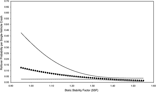
FIGURE 3-3 Estimated probability of rollover and 95 percent confidence intervals based on maximum-likelihood estimation of a logit model using data from six states for low-risk scenario. [NOTE: (STORM, FAST, HILL, CURVE, MALE, YOUNG, OLD, DRINK) = 00000010; 908 observations (0.4 percent of total) and 28 rollovers.]
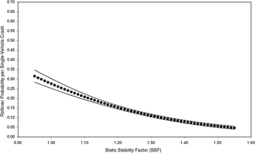
FIGURE 3-4 Estimated probability of rollover and 95 percent confidence intervals based on maximum-likelihood estimation of a logit model using data from six states for 25th-percentile–risk scenario. [NOTE: (STORM, FAST, HILL, CURVE, MALE, YOUNG, OLD, DRINK) = 00001100; 8,101 observations (3.9 percent of total) and 1,082 rollovers.]
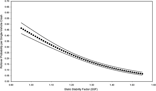
FIGURE 3-5 Estimated probability of rollover and 95 percent confidence intervals based on maximum-likelihood estimation of a logit model using data from six states for mean-risk scenario. [NOTE: (STORM, FAST, HILL, CURVE, MALE, YOUNG, OLD, DRINK) = 11000000; 3,346 observations (1.6 percent of total) and 694 rollovers.]

FIGURE 3-6 Estimated probability of rollover and 95 percent confidence intervals based on maximum-likelihood estimation of a logit model using data from six states for median-risk scenario. [NOTE: (STORM, FAST, HILL, CURVE, MALE, YOUNG, OLD, DRINK) = 01001000; 9,256 observations (4.5 percent of total) and 2,030 rollovers.]
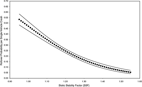
FIGURE 3-7 Estimated probability of rollover and 95 percent confidence intervals based on maximum-likelihood estimation of a logit model using data from six states for 75th-percentile–risk scenario. [NOTE: (STORM, FAST, HILL, CURVE, MALE, YOUNG, OLD, DRINK) = 11101000; 2,594 observations (1.3 percent of total) and 677 rollovers.]
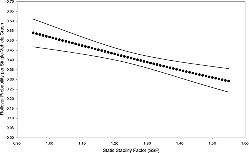
FIGURE 3-8 Estimated probability of rollover and 95 percent confidence intervals based on maximum-likelihood estimation of a logit model using data from six states for high-risk scenario. [NOTE: (STORM, FAST, HILL, CURVE, MALE, YOUNG, OLD, DRINK) = 01011001; 1,270 observations (0.6 percent of total) and 537 rollovers.]
NONPARAMETRIC MODEL
The confidence intervals calculated for the rollover curve using the logit model assume that the logit model is correctly specified. If the functional form of a model is incorrectly specified, the analysis based on confidence intervals may be misleading. The question addressed in this section is whether the logit model provides a satisfactory approximation to the true rollover curve. This amounts to asking whether F (see Equation 1) is indeed the cumulative distribution function of the logistic distribution or some other function.
The true, but unknown, functional form can be estimated using a non-parametric binary-response model—a model in which the functional form F is not assumed to be known. Hence, it is of interest to compare the estimated logit model with the estimated nonparametric model. The objective of this comparison is to reveal the extent to which the logistic cumulative distribution function provides a good approximation of the true, but unknown, functional form.
Estimation of the nonparametric model is challenging because it involves estimating the unknown functional form using the data. The non-parametric rollover curve was estimated by kernel regression, a well-known nonparametric estimation method. This method is discussed briefly by Greene (2000, 844–846); a more detailed exposition is found in Härdle (1990). In this section, the nonparametric estimation is illustrated using the binary data for Florida only. This nonparametric analysis was performed for illustrative purposes using a subset of the available data. A more extensive analysis using a larger dataset will be required if the nonparametric model is to be used to obtain a rollover curve that provides information at the national level.
Figure 3-9 presents the nonparametric estimate of the rollover curve and uniform 95 percent confidence intervals. This figure shows that an increase in SSF reduces the probability of rollover. The estimated rollover curve based on the logit model appears to be a reasonable approximation to the nonparametric-based rollover curve using limited data, suggesting that the logit model is a sensible starting point for constructing a rollover rating system.
ROLLOVER CURVE AND STAR RATING SYSTEM
NHTSA derived its five star rating categories for rollover resistance from the estimated rollover curve shown in Figure 3-1. Two features of the agency’s approach are of concern:
-
The lack of accuracy resulting from the representation of a continuous curve by an overly coarse discrete approximation, and
-
The lack of resolution resulting from the choice of breakpoints between star rating categories.
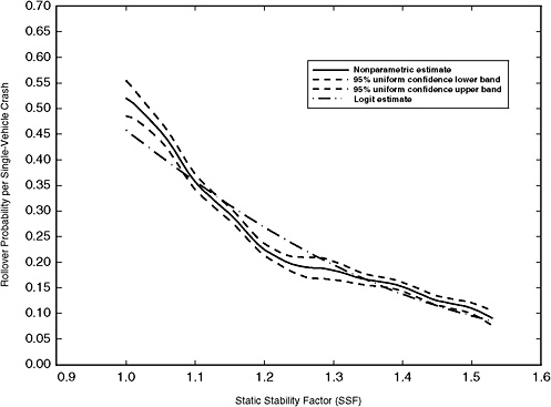
FIGURE 3-9 Nonparametric estimate of probability of rollover using a quartic kernel with a bandwidth of h = 0.07, n = 37,680. (NOTE: Both the logit and nonparametric curves illustrated in this figure are for Florida only.)
These related problems of accuracy and resolution need to be addressed in developing future consumer information on rollover to provide consumers with more useful and practical advice, commensurate with the evidence from real-world crash data.
Accuracy
The approach adopted by NHTSA was to approximate a continuous curve— the estimated rollover curve—by a discrete approximation comprising five levels, or star rating categories. This is a coarse approximation that results in a substantial loss of information, particularly at lower SSF values where the rollover curve is relatively steep. A more accurate approximation of the continuous rollover curve would use more levels. There would still be artificial jumps at the breakpoints between the levels, but this is an inherent feature of all such discrete rating systems.
Figures 3-10 and 3-11 show two examples of defining breakpoints on the SSF axis. The first figure is an example of a coarse four-step approximation to the estimated curve—the lines are drawn at 10, 20, and 30 percent. The horizontal lines drawn at these points define four bands of SSF values. Note that these bands are not of equal width since the curve is not a straight
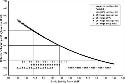
FIGURE 3-10 Example of using four SSF categories based on the model in Figure 3-2.
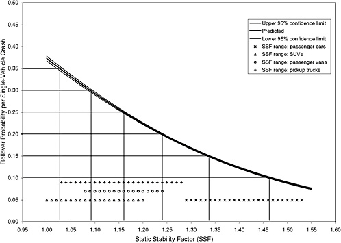
FIGURE 3-11 Example of using seven SSF categories based on the model in Figure 3-2.
line at a 45-degree angle. Figure 3-11 shows six lines drawn horizontally at 10, 15, 20, 25, 30, and 35 percent. These lines provide a finer resolution on the SSF axis with seven bands. Of course, the more bands there are, the closer is the approximation to the curve.
Resolution
A further problem with the star rating categories derives from the decision to select the breakpoints between categories by dividing the probability axis of the rollover curve into four equal 10-percentage-point probability intervals, plus one additional interval above 40 percent probability. The first interval represents rollover probabilities of 0–10 percent (five stars), the second represents probabilities of 10–20 percent (four stars), and so on up to probabilities greater than 40 percent (one star). However, equal intervals on the probability axis do not produce equal intervals on the SSF axis because the rollover curve is not a straight line, and its slope changes with changing SSF.
One important consequence is that the SSF intervals in the lower SSF range (up to approximately 1.25), where rollover probability changes quite rapidly with changing SSF, are too wide to permit discrimination among vehicles, even though analysis using the logit model indicates that such discrimination is statistically meaningful on the basis of real-world crash experience. The choice of breakpoints for the rating system does not exploit the richness of the available data, and consequently the rating system is not as informative as it could be. For example, the rollover resistance ratings for both SUVs and passenger sedans each span two rating categories: SUVs receive either two- or three-star ratings, whereas passenger sedans receive four- or five-star ratings. However, SUVs are more susceptible to rollover than are passenger sedans, and the rate of reduction of rollover probability with increasing SSF is greater for SUVs. The lack of resolution for vehicles with higher rollover risk detracts from the usefulness of the rating system, and a finer distinction among the rollover propensities of SUVs could be helpful in informing vehicle purchase decisions. Alternatively, as noted in Chapter 4, it may be possible to avoid the use of categories altogether. This could be achieved by presenting the actual SSF values or rescaled SSF values—for example, on a scale of 0–100.
FINDINGS AND RECOMMENDATIONS
Findings
|
3-1. |
Analysis of single-vehicle crash data indicates that an increase in SSF reduces the likelihood of rollover. |
|
3-2. |
NHTSA’s implementation of an exponential model does not provide sufficient accuracy to permit discrimination of the differences in rollover risk associated with different vehicles within a vehicle class. |
|
3-3. |
The relation between rollover risk and SSF can be estimated accurately with available crash data and software using a logit model. |
|
3-4. |
Given the richness of the available data, nonparametric analysis can provide a closer approximation of rollover risk. |
|
3-5. |
The current practice of approximating the rollover curve with five discrete levels does not convey the richness of the information provided by available crash data. |
Recommendations
|
3-1. |
Instead of using an exponential model, NHTSA should use a logit model as a starting point for analysis of the relation between rollover risk and SSF. |
|
3-2. |
For future analysis of rollover risk, NHTSA should employ non-parametric methods. |
|
3-3. |
NHTSA should consider a higher-resolution representation of the relation between rollover risk and SSF. |
REFERENCES
Abbreviation
NHTSA National Highway Traffic Safety Administration
Donelson, A.C., and R.M. Ray. 2001. Motor Vehicle Rollover Ratings: Toward a Resolution of Statistical Issues. Exponent Failure Analysis Associates, Inc., Menlo Park, Calif.
Federal Register. 2000. Consumer Information Regulations; Federal Motor Vehicle Safety Standards; Rollover Prevention; Request for Comments. Vol. 65, No. 106, June 1, pp. 34,998–35,024.
Federal Register. 2001. Consumer Information Regulations; Federal Motor Vehicle Safety Standards; Rollover Prevention; Final Rule. Vol. 66, No. 9, Jan. 12, pp. 3,388–3,437.
Greene, W. H. 2000. Econometric Analysis, Fourth Edition. Prentice-Hall, Inc., N.J.
Härdle, W. 1990. Applied Nonparametric Regression. Cambridge University Press, Cambridge, U.K.
NHTSA. 1999. Passenger Vehicles in Untripped Rollovers. Research Note, National Center for Statistics and Analysis.


