
1
The Role of Prediction in Paleoclimatology
JOHN IMBRIE
Brown University
INTRODUCTION
In the early, descriptive phase of any historical science, such as paleoclimatology, the primary task is to provide a narrative of past events. As facts accumulate, investigation enters an interpretive phase in which attempts are made to explain why these events occurred. Initially, these explanations are likely to be ad hoc in nature, verbal in form, and therefore difficult to pin down and test. Gradually, as data accumulate and as physical insights into causal mechanisms improve, it may be possible to transform such qualitative explanations into a numerical model of the natural system in which specific responses (system output) can be estimated from a knowledge of specific forcing functions (system input). The model can then be used to make hindcasts, i.e., to make predictions of system behavior over some past interval of time for which the forcing functions are known. The principal value of such a model is that the concepts on which the model is based can be tested by comparing hindcasts with observations. The test is particularly powerful if comparisons are made over an interval of time that was not used to develop the model.
In some cases it is possible to use a quantitative model to make forecasts, i.e., to make predictions of system behavior over some future interval of time. In order to use a model in this forecast mode, one must either be able to predict what values the forcing function will assume in the future or be investigating a system in which the behavior at any given time is strongly conditioned by previous values of a forcing function.
For many years, the science of paleoclimatology has been in a descriptive phase. But as other chapters in this volume make clear, the field has already begun to move into an interpretive phase. So far, however, most interpretations are formulated as verbal narratives rather than as quantitative predictions. The aim of this chapter is to point out the value of building paleoclimatic models that are capable of making quantitative predictions and to foster the development of such models by reviewing some of the types of quantitative, predictive models that have been used in climatology.
The first section of this chapter is a brief review of the nature of the climate system. The second section considers some general properties of quantitative, deterministic models. In the last section, six examples of quantitative climatic predictions are cited.

FIGURE 1.1 A simple model of the climate system illustrating internal and external sources of climatic variation.
THE CLIMATE SYSTEM
In order to formulate a predictive climate model it is necessary to have in mind some clear definition of the climate system. A conventional and useful definition (Figure 1.1) considers the climate system to consist of four interacting components; the atmosphere, the ocean, the cryosphere, and the surface of the land, including the terrestrial biota (NRC Panel on Climatic Variation, U.S. Committee for GARP, 1975). For simplicity, the last of these components is not shown in Figure 1.1, and the other components are not subdivided. The system boundary conditions are defined as the global geography, the geometry of the Earth’s orbit, the output of the Sun, and the concentrations of carbon dioxide and dust in the atmosphere. Two of these variables—orbital geometry and solar output—are clearly external to the climate system by any definition, because the values they assume are not influenced by the climatic state. However, some aspects of global geography—notably sea level and the elevation of the crust in high latitudes—are not completely independent of climate, so that the listing of geography as an external boundary condition makes sense only if the term is defined as the location of continents and oceans. Finally, we should note that the atmospheric concentrations of carbon dioxide and dust depend to some extent on the climatic state and are therefore not, strictly speaking, external variables. They are often placed in that category for the convenience of modelers, however.
Based on the definitions discussed above and illustrated in Figure 1.1, two quite different sources of climatic variation can be recognized (Mitchell, 1976). One of these sources is a change in external boundary conditions. Any such change will force the system as a whole to move toward a new equilibrium state and will therefore give rise to variations in the cryosphere, ocean, and atmosphere. This kind of climatic variation is described as being externally forced. Another type of climatic variation originates within the climatic system itself owing to interactions among the components of the system. These variations are internally forced and will occur even if all the external boundary conditions are fixed.
PROPERTIES OF DETERMINISTIC CLIMATE MODELS
From the above comments about the structure of the climate system, it is clear that the task of making quantitative predictive models is a challenging one (see Schneider and Dickinson, 1974, and Leith, 1978, for useful reviews). In general, there are two types of predictive models, deterministic and stochastic (Mitchell, 1976). Deterministic models view changes in one or more components (or subcomponents) of the climate system as forced by (1) changes in other components or (2) changes in external boundary conditions. Moreover, such models assume that the actual climatic narrative—the time-dependent behavior of the system component being modeled— can be predicted from a knowledge of changes in other internal components or from a knowledge of changes in external boundary conditions. Stochastic models, on the other hand, assume that random variations of internal origin make it impossible to predict the time-dependent behavior of the system. Instead, they make statistical predictions concerning the amount of variability to be expected over particular frequency bands (Hasselmann, 1976; Frankignoul and Hasselmann, 1977).
This chapter will discuss only deterministic models. Before proceeding, we examine some general elements of modeling strategy (Table 1.1). For example, in certain deterministic models the forcing function is identified as a change in one or more external boundary conditions (e.g., a change in global geography or orbital geometry). In other models, however, a change in one component of the climate system (e.g., atmospheric temperature) is viewed as a response to a change in another component (e.g., the sea-surface temperature or the extent of ice sheets), without taking feedback relationships
TABLE 1.1 Some Properties of Deterministic Climate Models
|
Category |
Possible Modeling Strategies |
|
Nature of forcing |
External or quasi-external |
|
Type of response |
Equilibrium or time-dependent |
|
Prediction mode |
Hindcast or forecast |
|
Mathematical form |
A wide range from simple, highly parameterized models to complex statistical-dynamical models |
between the prescribed variable (the predictor) and the calculated response (the predictand) into account. This type of forcing will be referred to as quasi-external forcing.
Another distinction to be made between modeling strategies has to do with the type of response. In many cases the response calculated is an equilibrium response to some specified change in an external or quasi-external forcing function. In this type of model, attention is focused on the new equilibrium value rather than on the time-dependent nature of the change to the new equilibrium. Such a formulation is reasonable provided that the characteristic time scale of changes in the forcing function is much longer than the characteristic time scale of the response. However, when these two time scales are of the same order of magnitude, so that the response never has a chance to approach equilibrium values, it is desirable to use a time-dependent model in which the response is explicitly calculated as a function of time. Such time-dependent models are sometimes referred to as differential models (Imbrie and Imbrie, 1980).
As previously discussed, predictions can be made in either the hindcast or forecast mode, depending on whether the changes modeled have actually occurred.
Finally, we should note that a wide variety of mathematical procedures are used in climate modeling. For many purposes it is useful to consider this variety as ranging across a wide range of complexity, from simple statistical models at one end of the scale to complex, statistical-dynamical models at the other. The simplest models make little demands on our knowledge of the underlying physics. The investigator is content to assume that the response being modeled is linearly related to one or more input variables, and his modeling strategy is to use regression methods to extract the constants of proportionality from a given set of data. As knowledge of the underlying mechanisms becomes more secure, the investigator may attempt to capture certain elements of the physical processes in a small number of differential equations, leaving the balance to be treated as statistical parameterizations. Such models of intermediate complexity predict the behavior of only a small number of climatic variables. At the other end of the range of complexity, more of the underlying physics is explicitly captured in differential equations, and fewer processes are treated statistically. Examples include the general-circulation models of the atmosphere, which take a global array of seasonal input parameters and calculate the seasonal response in three dimensions (Gates, Chapter 2 in this volume, 1976a, 1976b; Manabe and Hahn, 1977).
EXAMPLES
Examples to illustrate some of the modeling strategies already in use are given in Table 1.2. Donn and Shaw (1977) predict the atmospheric temperature field as a response to changing global geography since the Triassic (Figure 1.2). Imbrie and Imbrie (1980) hindcast late Pleistocene glacial history and forecast the glacial history of the next 100,000 years. Their model is shown in Figures 1.3 and 1.4. Gates (1976a, 1976b) and Manabe and Hahn (1977) have used estimates of ice-sheet distribution and sea-surface temperatures at the last glacial maximum, 18,000 years ago, as a basis for calculating the equilibrium response of the global atmosphere. Namias (1980) uses information on Pacific sea-surface temperature, and other information, to forecast weather patterns over the United States one season in advance. Barnett (1981) uses information on the Pacific wind field to hindcast sea-surface temperature off Peru, 12 months in advance (Figure 1.5).
TABLE 1.2 Examples of Climate Prediction Using Quantitative, Deterministic Models
|
Type of Forcing |
Predictor (Characteristic Time Scale in Yearsa) |
Predictand (Characteristic Time Scale in Yearsa) |
Reference |
Prediction Mode |
Type of Model |
|
External |
Global geography (107) Orbital geometry (104) |
Atmospheric temperature field (10−1) Global ice volume (104) |
Donn and Shaw (1977) Imbrie and Imbrie (1980) |
Hindcast Hindcast, forecast |
Complex equilibrium Simple time-dependent |
|
Quasi-external |
Global SST field Ice sheets (104) |
Global atmospheric fields of T, SST, winds (10−1) |
Gates (1976b); Manabe and Hahn (1977) CLIMAP Project Members (1976; in press) |
Hindcast |
Complex equilibrium |
|
Quasi-external |
Pacific SST (10−1) Pacific wind field (10−1) |
U.S. weather (10−1) SST off Peru (10−1) |
Namias (1980) Barnett (1981) |
Forecast Hindcast |
Simple time-dependent Simple time-dependent |
|
aT, temperature; SST, sea-surface temperature. |
|||||
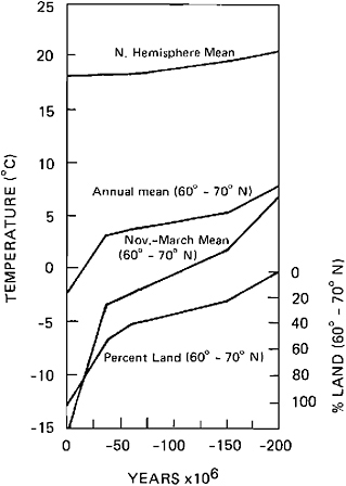
FIGURE 1.2 Change in mean temperature for the northern hemisphere (upper curve) and 60–70° N latitudinal zone (middle curves) computed for the past 200 m.y. Lower point for present on hemispheric curve is based on actual unaveraged grid-point data. Other curves are based on zonal means for land and water, respectively. Lower curve shows percentage of land in 60–70° N latitudinal zone (from Donn and Shaw, 1977, with permission of the Geological Society of America).

FIGURE 1.3 Response characteristics of a simple model for predicting global ice volume as a function of changes in orbital geometry. The response function has a mean time constant of 17,000 years and a ratio of 4:1 between the time constants of glacial growth and melting. Lower curve shows the system response to an arbitrary step input (Imbrie and Imbrie, 1980, copyright 1980 by the American Association for the Advancement of Science).
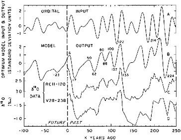
FIGURE 1–4 Hindcasts and forecasts of global ice volume derived from the response model shown in Figure 1.3. A, Input to the model. This curve represents changes in the incoming radiation during July at 65° N. B, Model output. C, Oxygen isotope curve for deep-sea core RC11–120 from the southern Indian Ocean. D, Oxygen isotope curve for deep-sea core V28–238 from the Pacific Ocean. Curves C and D are taken as estimates of changes in the global volume of land ice (Imbrie and Imbrie, 1980, copyright 1980 by the American Association for the Advancement of Science).
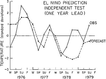
FIGURE 1.5 Observed and predicted values of sea-surface temperature off Peru (Barnett, 1981). The model uses variations in the Pacific wind field as input and is calibrated for the period 1950–1975. Thus Barnett considers the predictions as forecasts, whereas in this chapter they are defined as hindcasts. Unpublished work by T.P.Barnett, Scripps Institution of Oceanography, shows that the predictions are considerably improved if the assumption of stationarity of the seasonal signals is removed.
CONCLUSIONS
The examples of climatic hindcasting and forecasting reviewed in this paper are cited not because they solve fundamental problems in paleoclimatology, but because they illustrate a powerful method of attack on those problems: the formulation and testing of numerical, predictive models. So long as our explanations for past climates remain essentially qualitative in form, causal theories will be difficult to evaluate. It will, for example, be difficult to distinguish causal relationships from mere correlations and perhaps impossible to assess the relative importance of different causes that act together to produce a given effect. These problems are particularly acute in pre-Pleistocene climatology. Here it is often tempting to explain a given climatic change in terms of a correlated change in some particular aspect of the geometry of continents and oceans—ignoring other aspects of that geometry and implicitly denying the possibility that changes in atmospheric chemistry, in solar output, or in other climatic boundary conditions may be involved.
In the rapidly developing and challenging field of paleoclimatology, there is clearly an urgent need to test our ideas about the underlying physical mechanisms by developing quantitative, predictive models. As such models are substituted for the evasive verbal narratives that now serve as explanations of past climates, the science of paleoclimatology will come of age.
REFERENCES
Barnett, T.P. (1981) On the predictability of ocean/atmosphere fluctuations in the tropical Pacific, J. Phys. Oceanogr. 11.
CLIMAP Project Members (1976). The surface of the ice-age Earth, Science 191, 1131–1137.
CLIMAP Project Members (in press). Seasonal reconstructions of the Earth’s surface at the last glacial maximum, Geol. Soc. Am. Map and Chart Series, No. 36.
Donn, W.L., and D.M.Shaw (1977). Model of climate evolution based on continental drift and polar wandering, Geol. Soc. Am. Bull. 88, 390–396.
Frankignoul, C., and K.Hasselmann (1977). Stochastic climate models, part II. Application to sea-surface temperature anomalies and thermocline variability, Tellus 29, 284–305.
Gates, W.L. (1976a). Modeling the ice-age climate, Science 191, 1138–1144.
Gates, W.L. (1976b) The numerical simulation of ice-age climate with a global general circulation model, J. Atmos. Sci. 33, 1844–1873.
Hasselmann, K. (1976). Stochastic climate models, part I. Theory, Tellus 28, 473–485.
Imbrie, J., and J.Z.Imbrie (1980). Modeling the climatic response to orbital variations, Science 207, 943–953.
Leith, C.E. (1978). Predictability of climate, Nature 276, 352–355.
Manabe, S., and D.G.Hahn (1977). Simulation of the tropical climate of an ice age, J. Geophys. Res. 82, 3889–3911.
Mitchell, J.M. (1976). An overview of climatic variability and its causal mechanisms, Quat. Res. 6, 481–493.
Namais, J. (1980). The art and science of long-range forecasting, EOS Trans. Am. Geophys. Union 61, 449–450.
NRC Panel on Climatic Variation, U.S. Committee for GARP (1975). Understanding Climatic Change: A Program for Action, National Academy of Sciences, Washington, D.C., 239 pp.
Schneider, S.II., and R.E.Dickinson (1974). Climate modeling, Rev. Geophys. Space Phys. 12, 447–493.


