
4
Economics of Renewable Electricity
The previous chapters established the availability of renewable resources and outlined the technology options for converting those resources into electricity. This chapter explores the challenges and opportunities for bringing substantial renewable electricity generation to market to serve future U.S. electricity needs. Given the experience with renewables over the past 20–30 years, there is an inherent understanding that the economics of renewables have not been favorable. The economics of renewables is about profitability, and profitability depends on three drivers: (1) the market price or value of renewable electricity; (2) the costs of renewables relative to those of other energy resources; and (3), importantly, policies to promote renewables and environmental goals (particularly climate and energy security policies) that raise costs of using fossil fuels and/or subsidize costs of renewables.
The economic future for renewables depends on how market price, costs, and policy evolve. This chapter examines these drivers, the factors that underlie them, and issues associated with making predictions about them and their effects on the success of renewables in the marketplace. It sets out the fundamentals of the electricity market, explores technical and regional issues that affect renewables economics, and outlines the many entities engaged in renewable generation and what they bring to the table. The chapter concludes by summarizing and analyzing cost estimates for the renewable technologies with the greatest likelihood of contributing significantly to electricity generation in the next decade. The goal is not only to compare the costs of various technology options and how they will evolve over time, but also to clarify how markets and government actions can affect the near-term deployment of renewables.
This chapter focuses on the renewable technologies that are closest to market and for which assessments of current and future costs are thus more readily available. These include biomass, wind, concentrating solar power, solar photovoltaics, and geothermal (hydrothermal), but exclude traditional hydropower, because the potential for future extraction of this resource is limited, as noted in Chapter 2. The chapter also excludes hydrokinetics and enhanced geothermal technologies, which are still in the early stages of technological development. The costs presented here come from the wealth of data obtained from projects built in the recent past.
THE VALUE OF RENEWABLES
Predicting the economics of future renewable generation involves predicting the cost of generation from alternative sources and the value of electricity delivered to the marketplace. The competitive value would be the wholesale price of electricity for grid scale resources and something close to the retail price of electricity for distributed renewable resources.1 These prices define the value of adding renewables to the mix. The ability to predict electricity price is key to making predictions about future market penetration of renewable sources of electricity.
The value of generation from renewables will vary geographically and by time of day, because the marginal generator,2 which sets the electricity price, varies with location and over the course of the day with fluctuations in total electricity demand and available supply. Construction of more transmission facilities will increase the value of renewables by reducing transmission constraints between regions with abundant renewable resources and those with abundant load (Vajjhala et al., 2008).
The importance of relative costs means that efforts to understand how future expected declines in renewables cost are likely to affect renewables penetration will depend on future predictions of the market price of electricity. An analysis of the accuracy with which past studies from the 1970s and 1980s of several different renewable technologies—including wind, solar photovoltaics (PV), concentrating solar power (CSP), geothermal, and biomass—predicted future costs and future penetrations finds that these past studies performed reasonably well at predicting future cost declines but did not accurately predict market penetrations (McVeigh et al., 2000). McVeigh’s analysis shows that predictions consistently overestimated the expected retail price of electricity in future years. The renewable technologies included in the study had, for the most part, large reductions in cost over time, but these reductions were matched or exceeded by declines in the real cost of supplying electricity with fossil fuels, and thus renewables did not achieve predicted increases in penetration. This suggests that the challenge of predicting future costs of renewables may be exceeded by the challenge of predicting future market conditions that will confront those technologies, which will be equally if not more important in determining the ability of renewables to penetrate the market.
In addition to selling electric energy, most wholesale electricity markets also have an additional source of revenue from capacity payments. Capacity payments are made to encourage some generation to be readily available to meet changes in demand and ensure a high level of reliability in delivered electricity despite unforeseen outages. Requirements for the amount of capacity required vary regionally, but the value directly correlates to the expected performance of the unit when needed for generation. For dispatchable fossil generation and renewables, the capacity value is the highest, usually based on close to 100 percent of the unit’s rated capacity. For other renewables, the capacity value is typically lower to reflect the intermittent availability of the resource. The capacity value of a given renewable technology is regionally specific owing to how the capacity value is determined and the relative alignment between resource and load. Although intermittent, the capacity value of grid-scale solar would typically be higher than that of wind, because there is often better correlation between electricity demand and when the sun is shining. Solar resource availability is more predictable than wind is, though clouds do have a serious impact on solar flux. In a region where the wind resource availability does not correlate well with periods of system load, the capacity value may be as low as 8–10 percent of the rated capacity of the unit (ERCOT, 2007; GE Energy Consulting, 2005). In areas where resource or
transmission availability allows for better correlations with load, renewables will qualify for higher capacity payments. Capacity payments do not lower costs, but they affect the economics of renewables, because they provide an additional incentive to increase dispatchability.
Another source of value for most renewables3 is that their operation typically does not contribute to air pollution through emissions of NOx and SO2 and greenhouse gas (GHG) emissions, particularly emissions of CO2.4 Substituting renewable generation for fossil-fuel generation could reduce air pollution and greenhouse gas emissions. These benefits would depend on the type of fossil generation displaced, the emission controls on the fossil generation, the resulting emissions rate of that fossil generation, and the form of environmental regulation governing pollutants.5 For pollutants subject to an emissions cap, as is the case for SO2 nationally or CO2 in states participating in the Regional Greenhouse Gas Initiative, there will not be reduced emissions or environmental benefits. Emissions caps are both a ceiling and a floor on the level of emissions, as emissions reductions at one facility will be made up by increases at another facility, unless the cap is reduced or is no longer binding, which could occur with a dramatic increase in renewable generation.
If emissions are capped and emission trading is allowed, there could be an important effect on emission allowance markets and thus on the costs of electricity production from fossil fuels with greater penetration of renewables. Greater use of renewables could reduce demand for emission allowances for SO2 and NOx and other capped pollutants, which could reduce their allowance price. To the extent that renewables displace natural gas, at least initially, this effect is likely to be small for pollutants like SO2 and NOx. However, the effect could be larger for pollutants like CO2 if they were capped, though it is a value that would accrue to everyone who has to purchase allowances and not just to the utility that is adopting more renewables.
Most emissions of CO2 from electricity generators in the United States are not capped. Increasing renewables generation to replace fossil-fuel generation
|
3 |
With the exception of hydrothermal, which emits SO2 and CO2, and biopower, which emits NOx and CO2. |
|
4 |
There are emissions associated with the manufacture of different renewable technologies. These life-cycle effects are discussed in Chapter 5. |
|
5 |
Greater reliance on intermittent renewables like wind or solar could increase the need for spinning reserves from fossil generators, and increased operation of these generators in spinning mode or at less than full capacity could reduce the CO2 and NOx emissions benefits. |
would reduce CO2 emissions, at least relative to business-as-usual emissions. Identifying the extent of those reductions requires some caution. The effects would vary by location, based on the composition of the existing generation fleet and the types of new non-renewable generators and fuels that might otherwise be put in place to meet future electricity needs. These reductions in CO2 emissions would have value to society, and renewable generators might be able to capture some of that value if they could identify consumers willing to pay a premium for CO2-free electricity or green power.
COSTS AND ECONOMICS OF RENEWABLE ELECTRICITY
Cost is the principal barrier to the widespread adoption of renewable technologies. Generating electricity using renewable energy technologies is more costly than generating it with fossil fuels, especially coal, which supplies about half of the electricity generated in the United States each year. More transmission infrastructure in key locations would also be required for a dramatic increase in power supplied by renewables. Recent increases in renewables market penetration, particularly new wind power, have largely been in response to policies like the federal renewable energy production tax credit and state renewables portfolio standards. These policies seek to close the cost gap in the short term by subsidizing renewable generation. By encouraging greater market penetration, these policies enable reductions in long-term costs through increased scale and learning in manufacturing and in the use of the technology.
To achieve greater market penetration, renewables would have to undergo cost reductions at a rate greater than the rate of cost improvement by technologies that set the market price of electricity, including natural-gas- and coal-fired generation. These reductions might result from major breakthroughs in technology, improvements in manufacturing, or improved operating performance of equipment, such as higher capacity factors for wind turbines. Likewise, increases in the costs of fossil generation could have an impact on the relative competitiveness of renewables, though the magnitude might not be as great if cost increases also improved the competitiveness of energy efficiency options and nuclear generation.
Estimates abound of present and future costs for particular types of renewables and other sources of generation. Comparability of these estimates depends on the underlying assumptions and the types of costs captured in summary measures. The next sections discuss the types of costs associated with constructing and
operating renewable generating facilities, important assumptions underlying those costs, and how they can be used to construct summary measures of the cost of supplying energy.
Cost Concepts and the Levelized Cost of Energy
Developing a particular technology to generate electricity incurs costs for the capital equipment, such as the wind turbine and its tower, or solar panels; the land or property, if necessary for installation; and operating and maintaining the equipment. Some costs vary with the amount of electricity generated, and some costs are fixed. When a technology requires a fuel, such as biomass generation (biopower), the cost of the fuel would be a part of the variable operating and maintenance cost.
Capital costs do not vary with the amount of electricity generated by the facility and are typically stated in dollars per kilowatt ($/kW). Capital costs generally vary with the size of the facility or installation, with economies of scale or volume discounts on equipment orders favoring larger enterprises. Coal-fired and nuclear generating facilities exhibit economies of scale, and larger plants tend to have lower average cost of generation than smaller plants have. For renewables such as wind and solar PV, economies of scale can be greater at the equipment manufacturing stage than at the electricity-generating site, and increased capacity does not decrease the average cost of generation as much as it does for fossil and nuclear plants. Capital costs can also vary across sites, depending on land cost and the costs of installation or construction of the facility.
Fixed operating and maintenance (O&M) costs are also stated in dollars per kilowatt, but unlike capital costs, they are an ongoing expense associated with some unit of time ($/kW-year). Typically technologies are characterized by their annual fixed O&M costs. This category includes costs such as wages, materials, and land lease payments.
Variable O&M costs are typically expressed as dollars per megawatt-hour ($/MWh). Fuel costs can be expressed as dollars per unit of mass of the fuel ($/ton), dollars per unit of heat content of the fuel ($/Btu), or $/MWh. The last formula takes into account the efficiency of the technology in converting British thermal units (Btu) of heat input into megawatt-hours (MWh) of electricity.
In comparing the costs of generating electricity for different renewable technologies and for fossil fuels and nuclear technologies, cost estimates are typically converted into a levelized cost of energy (LCOE), which is expressed in $/MWh.
The initial cost of the capital equipment and installation constitutes a large portion of the cost of generating electricity, particularly for renewables, which have no fuel costs, with the exception of biopower generation. Converting this large up-front cost to cost per megawatt-hour requires making assumptions about the lifetime and capacity factor of the equipment,6 as well as the discount rate and the timing of returns on that capital. For intermittent technologies such as CSP, solar PV, and wind power, the capacity factor can vary considerably, depending on the location and the quality of the resource (e.g., wind speed and constancy for wind turbines, and hours of sunlight with no cloud cover for CSP and PV); likewise, the LCOE will vary depending on the capacity factor at a particular installation and location.
The cost of fuel plays an important role in calculating levelized cost for biopower. Biopower is typically a baseload technology with a high capacity factor. On an annual basis its fixed equipment costs could be recovered over many hours of operation. However, the hours of operation and the amount of electricity generated by biopower would depend on the cost of fuel, which accounts for about one-third of the total LCOE from biopower (Venkataraman et al., 2007). The cost of biomass fuel is uncertain and would depend on competing demands for crops and other agricultural inputs, including demands for biofuels from the transportation sector.
Costs Beyond Generator Costs
The costs of purchasing, installing, and operating a specific power plant might not be the total costs to the system and to electricity consumers of deploying a new renewable generation facility. Costs that might be missing from the traditional levelized cost measure include the costs of new infrastructure necessary to connect the renewable generator to the grid and to ensure continued quality of power supply. Other costs include up-front costs for approval of siting the new facility and costs for appraising the resource at the site, as well as costs of obtaining financing and environmental permits.7
Transmission
While fossil fuels may be transported from the mine or the wellhead to an electric generation facility, renewable generating plants must be located at or near the resource. There might be some degree of greater flexibility in location for biopower, but not much. It can be costly to ship biomass fuels, given the relatively low energy density compared to fossil fuels. Thus, biopower facilities are typically located close to sources of fuel.
Wind and some solar resources often are located at some distance from the existing transmission grid, and would require new transmission lines to transport the power to the centers of electricity demand or load. As with any new generation, the cost of constructing additional transmission lines should be included in the cost of supplying electricity from renewable resources. A recent report looked at 40 transmission studies covering a broad geographic area on the costs associated with the transmission requirements for wind power (Mills and Wiser, 2009). The transmission costs associated with wind ranged from $0 to $1500/kW, and the majority were less than or equal to $500/kW, with a median of $300/kW. These numbers correspond to $0–79/MWh, with the majority below $25/MWh, and a median of $15/MWh. Intermittent renewables generation requires an additional consideration. Because of low capacity factors, dedicated transmission lines sized to transmit the full amount of power produced during peak generation hours would be unused or underused some of the time. Siting additional peaking capacity along a new transmission corridor could potentially leverage the available transmission capacity during periods of underuse by the renewables.
A caveat to the preceding discussion is that distributed renewables, such as distributed PV, might end up closer to the load than conventional generation and could lead to less need for investment in transmission. To really achieve substantial benefits in terms of avoiding investment in transmission infrastructure may require substantial amounts of distributed renewables investment in particular locations.
Intermittency
At sufficiently high capacities of solar and wind generation, the costs of intermittency could extend beyond costs associated with dedicated transmission facilities to affect the operation of the interconnected transmission grid. More generation from intermittent resources will require additional or alternative resources to help track load, provide voltage support, and meet needs for capacity reserves.
These include demand for second-by-second electricity load balancing service, or regulation; load following within the hour; and unit commitment of generators to be available at particular times of the day or week. Renewable electricity must be used when generated because the electricity can be generated only when the resource is available. Typically, fossil-fuel generators that are easily dispatchable, such as natural gas combustion turbines, supply these ancillary services. As renewables generation increases and fossil generators are curtailed, renewable generation technologies themselves or additional system assets, such as storage, will be needed to meet the increased need for ancillary services, at some additional cost. When system managers have improved tools and technology for predicting resource availability, it will be easier to determine the need for additional generation resources to back up intermittent renewables. Smart Grid technologies, which allow system managers to manage supply and demand in real time, could also mitigate some of the costs of renewable intermittency. An upgrade and expansion of the electricity grid will be necessary no matter what happens with renewables, given the age of the grid and the anticipated growth in electricity demand.
Studies in the past five years looked at the costs of integrating wind into the grid, as summarized in Figure 4.1 (Smith, 2007; Wiser and Bolinger, 2008). These
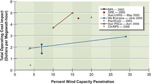
FIGURE 4.1 Summary of wind plant ancillary services costs from various studies looking at the cost of regulation service, load following, unit commitment, and natural gas.
Source: Developed from data in Smith (2007) and in Wiser and Bolinger (2008).
studies examined the costs of regulation service, load following, unit commitment, and natural gas and found that the incremental costs per megawatt-hour range from about $1.50 to almost $5.00. A study on using wind to serve 50 percent of demand showed that the incremental costs are $10–20/MWh, including transmission, storage, and backup generation (DeCarolis and Keith, 2004). The European Wind Energy Association conducted a study of more than 180 sources and determined that additional costs range from $1.50 to $10.20/MWh for market penetration levels of 10 percent and from $2.80 to $11.50 for higher penetration levels (EWEA, 2005). Typically the predicted costs are higher in studies that focus on higher market penetration of wind. In the studies on different levels of penetration, the costs were higher with the higher levels of penetration, but the incremental effect of increased penetration varied across studies. Generally, where the average cost of wind generation would be about $80/MWh, the impact of grid integration costs appeared to be less than 15 percent where wind produced 20 percent or less of total electricity generation.
Energy Storage
Energy storage could mitigate the impact of intermittent renewables. Today there is very little storage in the United States, as high costs, low efficiencies, and technological uncertainty precluded storage from becoming economically viable.8 Costs for battery and other storage technologies are generally about two to five times higher than the cost target that would make them competitive (less than about $200/kWh for a 4-hour system) (Rastler, 2008). However, technologies might be called on in the future to store electricity generated from intermittent renewable resources if their combined market penetration would rise to 20 percent and beyond.
Efficient, cost-effective energy storage could promote grid-scale renewable electricity. Wind and solar system operators have limited control over the amount and timing of power generation, and their production does not line up well with demand requirements. Storage would allow a grid operator to align the dispatch curve with the demand curve, a process referred to as load shifting. In addition to generating revenue when the wholesale market is at its peak, the ability to draw
on storage would obviate the need for some peaker generators at the margin. Storage would also alleviate the reliability concerns associated with wind and solar. When renewables provide less than forecasted output, the operator has to turn to the spot market or bring on idle combined cycle natural gas generators to make up the difference. Conversely, when renewables provide too much power, those holding day-ahead gas contracts might not realize the value of their contracts. The market penalizes renewables for this uncertainty and, while recent studies have shown that this might not matter until intermittent renewables reach penetration levels in excess of 20 percent, this uncertainty may have to be addressed if they are to extend any further (DOE, 2008).
Storage would also mitigate some site limitations of renewable electricity and help reduce the size and increase the utilization of transmission lines installed for renewable sources. Small-scale domestic storage could also change the economics of distributed wind and solar generation, providing homes with energy security while perhaps making it possible to sell stored energy or capacity back to the grid. As plug-in hybrid electric vehicles (PHEVs) become a reality, households could store the energy they generate right on their vehicles. The National Renewable Energy Laboratory (NREL) found that PHEVs could enable increased penetration of wind energy (Short and Denholm, 2006).
Figure 4.2 displays how some of these storage technologies compare in terms of cost of energy and cost of power. At the grid-scale level (greater than 10 MW), compressed air energy storage (CAES) appears to be the most economical now, though the practicality of CAES also depends on the availability of suitable sites. Iowa Energy Storage Park (IESP), a 268 MW system, is scheduled to come on line in Iowa in 2011. Projected costs for IESP are $200–250 million, or $746–933/kW, and the system is designed to go from idle to full output in under 15 minutes. The Texas State Energy Conservation Office estimated total overnight capital costs of a new CAES system at $605/kW. Development and fixed O&M costs were listed at $28.00/kW and $14.07/kW, respectively, and variable O&M costs were estimated to be $1.50/MWh (Ridge Energy Storage, 2005). Batteries are modular and nonsite specific, which makes them ideal for distributed generation. The quick, cheap response time also makes batteries ideal for providing backup power, or uninterruptible power supply (UPS). Yet despite broad application in other sectors, batteries are still very expensive, as shown in Figure 4.2.
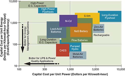
FIGURE 4.2 Storage technolgies and costs of energy and power.
Source: Electric Power Research Institute; presented in Rastler, 2008.
Financing Costs
Another element of cost that should be included when evaluating the overall competitiveness of any generation project is the cost of money. Because electricity generation projects are capital-intensive and have long lifetimes, access to capital and the rates at which it is paid back are key components of project cost. The magnitude of these costs differs, depending on the type of generation financed. For example, a renewable project that does not require fuel has a much larger portion of its costs associated with the initial capital expense of the plant than a gas-fired power project that will have greater operating expenses throughout its lifetime, even if both have similar LCOEs. These costs are project-specific, based on circumstances related to the project’s financing strategy, the maturity of the technology, and risk factors discussed in Chapter 6.
Financing of renewables projects differs from that of fossil-fueled plants. Although the total magnitude of capital may be smaller for a renewable project than for a fossil project, the capital intensity relative to operating costs is much higher for renewables without fuel, such as wind and solar. There is more up-front risk in the renewables project’s financial model. Further, the tax incentives
that could subsidize some renewables might not be directly available to the project developer and could require more complex financing structures to access the benefit. The project financing structure, such as the debt-to-equity ratio; the types and costs of loans, depending on the risk profile; and the magnitude and timing of returns to financing entities can have an impact of as much as $15/MWh on a wind project’s levelized cost of energy (Harper et al., 2007). Regional variability in the costs of land and logistical support and time variability in the selling price of electricity due to market forces complicate financing for renewables projects. For wind projects before the 2008–2009 economic crisis, the cost of tax equity appeared to decline by approximately 3 percent and interest rate margins on debt transactions by approximately 0.5 percent (Wiser and Bolinger, 2008). This trend toward cheaper capital resulted directly from reduced project risks as the wind power industry matured and the available capital for wind projects increased. Economic events dramatically reversed this trend for all forms of power generation but have affected renewables to a greater degree, due to the reliance on investor tax capacity in order to realize the economic benefit of the production tax credit (PTC). The American Recovery and Reinvestment Act of 2009 attempted to address this issue by allowing non-solar renewable electricity facilities to elect a 30 percent investment tax credit in lieu of the PTC.
Because of their small scale and modularity, advantages that wind and solar PV projects have over fossil projects is the shorter time between purchase of the equipment and placing it on line and the ability to start up the first few generators while others are under construction (Bierden, 2007; Royal Academy of Engineering, 2004; Sheehan and Hetznecker, 2008). These two features reduce the magnitude of draws on cash flow and accelerate the repayment of debt.
Methodologies for Projecting Costs
An overview of the different approaches to projecting future costs places the cost projections in this report in context. The panel identified three methods for predicting future costs of renewables.
The first methodology predicts the levelized cost of energy that must be achieved from a particular renewable generating source to be competitive with other sources of electricity by some date in the future. This method requires estimating the future wholesale market price of electricity with which renewable resources must compete. These predictions omit consideration of uncertainties, the relationship between government policy and expenditures, and changes in the
costs of using renewables to supply electricity. The Western Governors’ Association (WGA) Solar Task Force took this approach and developed a series of referent market prices that depend on the assumed price of natural gas, the energy source typically setting the market price of electricity in the western states (WGA, 2006b). The higher the predicted price of natural gas, the lower the cost reduction hurdle for renewable technologies.
A second approach that is similar to the first involves the enunciation of cost and technical performance goals, such as availability factors, that those researching future developments of the technology, such as the Office of Energy Efficiency and Renewable Energy (EERE) at the DOE, expect the technology to achieve as a result of their research program. The idea behind this approach is to establish goals for a research and development (R&D) program and also to provide some benchmark expectations about technological improvement that could be used later to judge the performance of the research program after the fact. This approach is used in NREL’s projections that it develops for DOE (NREL, 2007).
The Energy Information Administration (EIA) took a third approach to cost prediction in constructing a more formal model of how technical costs might evolve over time. Models can be based on a projection of past trends or a formal learning or technological improvement function. Cost reductions through learning are greater for new technologies than for mature technologies. EIA took the learning-curve approach to predict how costs would evolve as greater amounts of a particular technology penetrate the market in response to a combination of policies and electricity demand growth (EIA, 2007a). This is the approach underlying the cost estimates for EIA and the Electric Power Research Institute (EPRI) shown in Tables 4.A.1 and 4.A.2 in the annex at the end of this chapter.
Some might argue that present-day costs would be the best predictor of future costs, particularly in the short term. This approach might suffice for forecasting future costs for more mature renewable technologies such as wind, but might be less appropriate for nascent technologies. Another problem with this approach is that factors contributing to short-term cost increases, such as the recent increases in the cost of wind turbines and solar cells due to material shortages, might not be sustained into the future, as entry into the industry, greater availability of materials, and innovations might bring costs down.
POLICIES AND PRACTICES THAT AFFECT THE ECONOMICS OF RENEWABLE ELECTRICITY GENERATION
The United States and other nations have implemented policies to increase the market penetration of renewables. Typically these policies work by either subsidizing the cost of renewable generation (and thereby decreasing their relative costs) or by increasing the demand for renewable generation. Some policies provide for additional sources of revenue for renewable generators, such as through the sale of renewable energy credits. The form of the policy and the amount of the payment or subsidy for renewables are both determinants of the policy’s effect on renewables penetration.
The panel considers three classes of policies in this section: (1) policies and practices targeted at renewable technologies; (2) environmental policies that raise the cost of using conventional technologies, thereby improving the relative cost competitiveness of renewables; and (3) other electricity market policies that could affect the economics of using renewables and their ability to penetrate the future market.
Policies to Promote Renewables
Both the federal government and a majority of the states have policies to promote the use of renewable technologies to supply electricity. Most of these policies are described in Chapter 1. Here, the panel focuses on a few policies and describes how they appear to affect the economics of renewable generation. Some policies target large central station facilities, while others focus on distributed renewables intended for personal consumption. The following review focuses on the major policies in terms of their potential capability and their relevance for renewables market penetration.9
Production Tax Credits
A renewable energy production tax credit (PTC) policy allows firms that generate electricity with eligible renewable technologies to offset their income tax liability
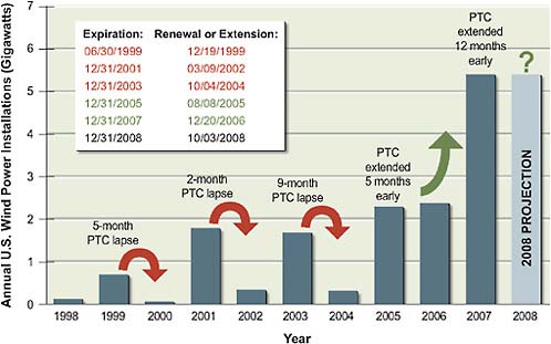
FIGURE 4.3 Effects of production tax credit expiration and extension on wind power investment. Not shown are the almost 8,400 GW of installed wind power in 2008 and the extension of the PTC until 2012.
Source: Lawrence Berkeley National Laboratory; presented in Wiser, 2008.
by the amount of the tax credit times the number of kilowatt-hours generated. The federal PTC applies to a range of renewable technologies, with some technologies, including wind, solar, closed-loop biomass, and geothermal, eligible for a larger tax credit than others, such as open-loop biomass, small hydroelectric, landfill gas, and municipal solid waste.10 Generators are eligible for the tax credit for every kWh of electricity generated during their first 10 years of operation. The federal renewables PTC policy was recently extended until 2012 and beyond, as described in Chapter 1. Initially passed in 1992, this policy typically had only been approved for 1–2 years into the future and lapsed three times since its inception. As shown in Figure 4.3, the intermittency of this policy led to large fluctua-
tions in demand for wind turbines as project developers raced to beat the deadline and then lost interest in new projects when the policy lapsed (Wiser, 2008).
In addition to the federal PTC, five states (Florida, Iowa, Maryland, Nebraska, and New Mexico) also offer PTCs that provide a tax credit for every kilowatt-hour of electricity generated. Another seven states offer direct payments for each kilowatt-hour of electricity generated by certain renewable technologies.
Both an investment tax credit (ITC) and a renewable PTC reduce the cost of generating electricity using renewables. The PTC is arguably more effective at getting performance out of a generator, because the level of the PTC subsidy depends directly on how much electricity the generator produces, whereas the ITC does not differentiate between a renewable that is productive and one that does not generate much electricity. However, using a tax credit based on electricity production may not be viable for distributed technologies owned and operated by end users. At present levels, the federal PTC reduces the cost of supplying renewables by 1–2¢/kWh, depending on the technology, divided by 1 minus the marginal income tax rate. The reason for the transformation is that the tax credit is equivalent to after-tax income. To earn 2¢/kWh in after-tax income, before-tax income would have to be greater than 2¢. Likewise, since a decrease in cost is the same as an increase in income, the decrease in before-tax costs that is equivalent to the 2¢ tax credit must be greater than 2¢. Thus, for companies in the 33 percent marginal tax bracket, this would be an increase of after-tax income of about 1.5 times the value of the tax credit, as that would be the increase in total revenue equivalent to the decrease in tax burden (assuming the affected firm still has a tax burden) (EIA, 2005).
Modeling analysis demonstrates the potential capability for an extended PTC to increase investment in and generation from eligible renewables. In response to a request from the House Committee on Ways and Means, EIA (2007b) analyzed the effects of both a 5-year and an indefinite extension of the PTC for wind generators only. This analysis considered the effects of a continued PTC for wind at 1¢, 1.5¢, and 1.9¢/kWh. The results suggest that extending the PTC at the current level for 5 years would lead to 30 percent more wind capacity in 2020 compared to the AEO 2007 forecast, and total wind generation equal to 1.5 percent of total generation in 2020, compared to a baseline share for wind of about 1 percent in 2020. Extending the PTC indefinitely would more than double the amount of wind capacity in 2020 compared to the AEO 2007 baseline and would almost triple it by 2030. These increases in investment and associated wind generation would have very little impact on the price of electricity to consumers, although
there would be a cost to the U.S. Treasury ranging from $2 billion, with a 5-year extension of the present credit, to more than $20 billion with a permanent extension.11
According to the EIA analysis, extending the PTC for only 5 years would have a negligible effect on CO2 emissions, largely because the displaced generation comes mostly from natural gas. However, with a permanent extension of the PTC, the investment in wind would displace more investment in new coal-fired generation, resulting in about a 2 percent reduction in CO2 emissions from the electricity sector compared to the AEO 2007 forecast in 2020. Palmer and Burtraw in an earlier study (2005) extended the PTC indefinitely to both wind and biopower and demonstrated a more substantial increase in renewables generation by 2020, and nearly 5 percent lower CO2 emissions in 2020 compared to a no-extension base case. Despite this substantial reduction in CO2 emissions, their work suggested that the PTC is not as cost-effective in limiting CO2 emissions as other policies, including renewable portfolio standards (RPS) or a CO2 cap and trade approach, which could achieve a similar reduction in CO2 emissions at much lower costs.
Renewable Portfolio Standards
As of 2008, the District of Columbia and 27 states have renewable portfolio standards (RPSs) that require a minimum percentage of electricity sold to customers within a state to be generated using renewable resources. An additional six states have voluntary programs. Details of all state RPSs can be found in Appendix D of the report. Figure 4.4 from the Lawrence Berkeley National Laboratories shows the timing of the adoption of RPS policies in different states and indicates that many states revised their policies after adoption, typically to make them more ambitious.
An RPS policy creates an increase in demand for electricity supplied by renewables and, in most cases, a demand for a complementary product that renewable generators can sell, a renewable energy credit (REC). RECs can be traded and bundled with the electricity that the generator produces or as an unbundled separate product. Revenue from the sale of RECs provides an additional incentive for renewable generators to supply electricity. Researchers at Lawrence Berkeley National Laboratory found that 60 percent of wind capacity
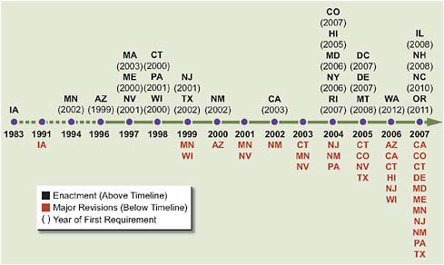
FIGURE 4.4 Renewable portfolio standards policy adoption and modification across the states.
Source: Wiser and Barbose, 2008.
constructed in 2006 was motivated at least partially by state RPS policies (Wiser and Bolinger, 2008).
The effects of a state RPS policy on the economics of renewable generation in particular and electricity supply more generally depend on features of the policy, including its stringency, what renewable technologies are included, site restrictions on renewables eligibility (e.g., limitations on out-of-state renewables), cost containment measures, and enforcement penalties. For example, a policy that caps the price of an REC at a low level or allows regulated electricity suppliers to make a small alternative compliance payment in lieu of meeting the RPS obligation would provide a weaker incentive for renewables development than would a policy that has no REC cap and stringent requirements for RPS compliance. State RPS policies differ dramatically in terms of features.12 Figure 4.5 shows how REC prices in various state programs for tier-one resources—the most valuable and flexible resources—have evolved since early 2003, and how prices differ across states. In general, prices in New England tend to be higher than prices in Texas
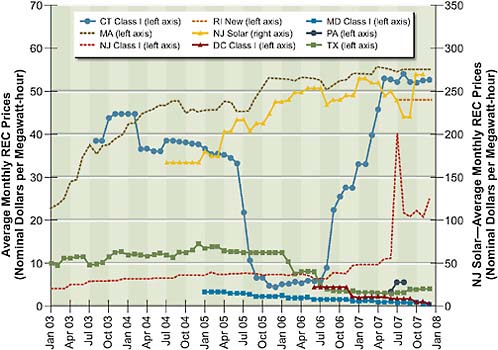
FIGURE 4.5 Renewable energy credit (REC) prices in the renewables portfolio standard compliance market.
Source: Wiser and Barbose, 2008.
and the mid-Atlantic states (with the exception of New Jersey solar). These differences reflect in part the difficulty in siting new renewable generators in New England. Fluctuations in REC prices over time within a state program reflect changes in state conditions. For example, large fluctuations in REC prices in Connecticut followed from changes in the states from which Connecticut electricity suppliers could purchase RECs and from imposing RPS requirements on municipal generators in 2007, which increased demand for Connecticut RECs. The states with the highest REC prices or with the highest RPS requirements in 2007 saw the largest impact on their electricity prices in that year.
A federally mandated RPS policy could reduce the differences in RPS policies across states. There have been unsuccessful attempts in Congress to pass a national RPS. EIA’s analysis of a federal policy mandating a 25 percent RPS and a 25 percent renewable fuel standard by 2025 suggested that a federal RPS of 25 percent would result in REC prices between $35 and $50/MWh in 2025, depending on assumptions about fuel costs and technology improvement (EIA,
2008b). The 25 percent RPS policy would result in about 20 percent lower annual CO2 emissions from the electricity sector than the AEO 2007 baseline in 2025. EIA’s earlier analysis of a 15 percent RPS showed that annual CO2 emissions from the electricity sector in 2030 could be 6.7 percent lower with such a policy than under a base case scenario (EIA, 2007c).13
Previous modeling of less stringent RPS policies suggested that the REC price is not a linear function of the level of the portfolio standard requirement. Instead, the REC price for a national policy seems to be an increasing function of the threshold, particularly for levels higher than 15 percent (Palmer and Burtraw, 2005). These models assumed that the federal standard would replace existing state-level RPSs. However, with a federally mandated policy in addition to existing state RPS policies, the price of a federal REC would tend to be lower and would depend on regional transmission capability to bring power from resource-rich areas to regions with high levels of electricity demand (Vajjhala et al., 2008).
Green Power Marketing
Green power marketing is the direct marketing of power generated by renewable resources and supplied directly to end users of electricity. Green power refers to all types of renewables except hydropower. Green power marketing typically focuses on selling power from new facilities. Green power marketing can occur in competitive electricity markets or as an elective tariffed service that regulated utilities offer rate-paying customers. According to researchers at NREL, voluntary purchases of green power represented about 32 percent of total green power generation in 2005 and about 36 percent of total green power generated in 2006 (Bird and Swezey, 2006; Swezey et al., 2007; Bird et al., 2007). In 2006, voluntary green power markets supplied about 12 billion kWh of generation out of a total demand of more than 3600 billion kWh.
As more and more states adopt RPS policies, the question arises as to whether these mandatory policies will replace voluntary markets for green power. A study of the relationships between mandatory RPS programs and voluntary green power markets found potential for overlap in the form of double-counting, which is selling renewable kilowatt-hours to voluntary markets and using the
same renewable kilowatt-hours to comply with an RPS (Bird and Lockey, 2007). Most states prohibit double-counting; in some states some amount is allowed. In others, there are no rules, and it is difficult to know if voluntary markets are producing more renewable generation. One benefit of voluntary green power markets is that excess renewable generation beyond that required for RPS compliance may be sold into the green power market, providing a way to manage timing inconsistencies and lumpiness in renewable resource development.14
Voluntary and compliance REC markets differ in that most compliance REC markets are limited in scope, while voluntary green power markets can be national in scope. This means that the relationships between prices of compliance RECs and voluntary RECs are often unrelated. The effects of an RPS on voluntary purchases of green power are difficult to identify, but analysis of data from four states that have both RPS policies and active green markets showed that voluntary green power sales have continued to increase after the adoption of the RPS policy (Bird and Lockey, 2007).
Renewable Feed-In Tariff
To encourage renewables, most European nations, including France, Germany, Spain, and Denmark, prefer not to set a relative quantity target as is done with an RPS. Instead, policy makers in these countries specify a minimum price, called a feed-in tariff, that utilities must pay generators for renewable electricity. The level of the feed-in tariff varies by technology and is calculated to ensure profitability of the generation regardless of its levelized cost of energy (LCOE). For example, solar power receives a much higher price than does wind. The tariff is guaranteed to be in place at a predetermined level for a statutorily defined time, enabling its benefit to be incorporated into the evaluation of renewable project financiers. To illustrate, the feed-in tariff in France for onshore wind provides €0.082/kWh for 10 years, followed by between €0.028 and €0.082/kWh for 5 subsequent years, depending on the site (IEA, 2006). Feed-in tariffs for solar PV tend to be substantially higher, ranging from a low level of €0.052/kWh in Estonia to as high as €0.60/kWh in Austria (Klein et al., 2006).
The feed-in tariff is typically funded by revenue collected from all electricity customers. The German government estimated that each German household
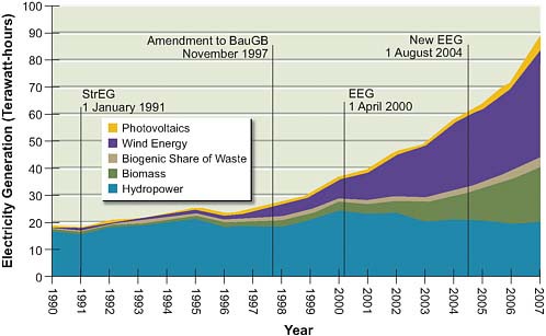
FIGURE 4.6 Growth in electricity generation from renewable energy sources in Germany.
Source: German Federal Ministry for the Environment, Nature Conservation, and Nuclear Safety, 2007.
paid an additional €2.10/month to cover the costs of the 53.4 TWh eligible for the tariff (German Federal Ministry for the Environment, Nature Conservation, and Nuclear Safety, 2007). The correlation between growth in renewables penetration, shown in Figure 4.6, and tariff eligibility is clear. In Germany the feed-in tariff for solar declined by 5 percent each year to reflect expected reductions in cost of solar panels due to learning. However, a government proposal called for a more dramatic reduction in tariff levels to help lower the costs of this policy. The anticipated cost reductions from increased production of solar PV had not materialized, and instead, shortages of high-grade silicon used in solar cell production resulted in more than a 10-fold increase in silicon prices since 2003 (Economist, 2008). The German experience with feed-in tariffs demonstrates the complexity of trying to influence the economics of a particular technology through policy.
Environmental Policies
Policies such as the Title IV cap and trade program for SO2 emissions raise the cost of fossil-fuel electricity generation and could potentially promote generation from renewables. This effect has been small for policies focused on criteria
air pollutants and mercury. Because there is a lack of tested cost-effective ways to reduce CO2 emissions directly from fossil generators, policies to cap emission of greenhouse gases may provide a stronger economic signal to adopt renewables. The success of that signal will depend on the stringency of the policy, the expected evolution of the policy over time, and the relative economics of demand-side alternatives.
Policies to Control Conventional Pollutants and Mercury
Policies to restrict emissions of SO2, NOx, and mercury from electricity generated from fossil fuels have had only a small effect on renewable generation. Fuel switching from high-sulfur coal to low-sulfur coal and installing post-combustion controls for reducing NOx emissions, such as selective non-catalytic reduction (SNCR), are more cost-effective than is switching from fossil-fuel generation to renewable generation. Modeling suggests that policies restricting emissions may produce a small increase in renewable generation, particularly if mercury emissions are being restricted (Palmer et al., 2007; EIA, 2004). For example, EIA’s study of the Clear Skies Act that placed caps on national emissions of SO2, NOx, and mercury found that capping emissions of these pollutants would result in 20 percent more generation by non-hydropower renewables in 2020 compared to the base case, raising the non-hydropower renewables generation’s share of the total electricity used in the United States from 3.0 percent in the base case to 3.6 percent in 2020. The economics of renewables appears to depend more on the price of natural gas or coal than on the stringency of policies to limit SO2, NOx, and mercury.
Policies to Limit Emissions of CO2
A host of approaches has been proposed for limiting emissions of CO2. The electric utility sector and other large stationary sources seem to prefer a CO2 cap and trade program, which has been adopted in the Regional Greenhouse Gas Initiative in the northeastern United States and has been implemented for large stationary and utility sources in the EU CO2 Emissions Trading Scheme. Several pieces of federal legislation in the 110th Congress proposed cap and trade programs. A cap on CO2 emissions might have a greater impact on renewables penetration than would caps on other pollutants, since direct abatement of CO2 emissions is not currently feasible. Until CO2 capture and sequestration becomes realistic and economic, reductions in CO2 emissions will come from generating with different fuels, includ-
ing renewables; more efficient operation of existing emitting facilities; and more efficient electricity consumption. A CO2 cap would raise the cost of using fossil fuels, in turn raising the market price of electricity, which could have positive effects on the profitability of renewables. The effect of different prices of CO2 on the LCOE of coal- and natural-gas-generated electricity is shown in Table 4.1.
The EIA provides insight into how climate policy might affect investment in renewables technologies in its study of the Bingaman-Specter proposal to cap economy-wide CO2 emissions near the 2006 levels in 2020 and 1990 levels in 2030. This bill also includes a cap on the price of CO2 emission allowances of $15 in 2020 that rises to $25 by 2030. Under this policy, investment in new non-hydropower renewable generating capacity would either double or triple in 2020 in response to the policy relative to baseline levels, depending on underlying cost and performance assumptions. However, the share of electricity provided by renewables including hydropower would only increase from 10 percent in 2007
TABLE 4.1 2020 Cost Projections of Electricity from Fossil Fuel with CO2 Tax, from AEO 2009 Reference Case (in 2007 dollars)
to 15 percent by 2020 (EIA, 2008a); non-hydropower renewables would increase from 3 percent to approximately 9 percent of electricity generation. In analyzing the more stringent Lieberman-Warner proposal, EIA concluded that with a CO2 allowance price of about $48 in 2025, the amount of generation from non-hydropower renewables would more than quadruple in 2025 relative to the no-climate-policy baseline scenario and would climb to more than 13 percent of total generation in that year (EIA, 2008a).
Some policies to reduce CO2 could have the perverse effect of limiting the ability of those seeking to market renewable energy directly to consumers to make environmental claims about the emissions consequences of switching to renewable power. Because a cap on emissions of CO2 is both a ceiling and a floor, increased generation from renewables would free up a CO2 allowance for use elsewhere. To support voluntary renewables markets, several states participating in the Regional Greenhouse Gas Initiative plan to retire CO2 allowances in connection with voluntary sales of green power to maintain the opportunity for credible green power claims.
Other Types of Policies
Time-of-Use or Real-Time Pricing
Time-of-use or real-time pricing of electricity can affect incentives for the installation of distributed renewables such as solar PV. If peak demand times or peak-load pricing coincide with the times of availability for solar PV or other distributed renewables, more widespread use of time-of-day or real-time pricing could encourage the development of renewables, particularly when peak period price is several times higher than base period price for electricity. For example, with real-time pricing, the value of electricity from PV in California is 30–50 percent higher than in the absence of real-time pricing (Borenstein, 2008a). The effect of a shift to real-time pricing on the value to electricity consumers of installing PV would depend on how electricity prices were set in the absence of real-time metering. For example, the tiered structure of flat electricity rates in the Southern California Edison territory, which led to higher electricity prices for heavy-use consumers, meant that the value of PV installation was higher for many customers under a flat-rate structure than with real-time pricing (Borenstein, 2007).
Advanced meters that keep track of electricity use in real time are a prerequisite for real-time pricing. A study by the Federal Energy Regulatory Commission (FERC, 2006) found that only about 6 percent of customers nationwide had the
advanced meters necessary for real-time pricing, but in some parts of the country as many as 15 percent of the customers had these meters.
Conversely, time-of-use pricing could actually make grid-scale solar less attractive to investors. Time-of-use pricing would tend to flatten the load curve, reducing the market clearing wholesale price of electricity during peak hours. To the extent that these hours coincide with solar generation, this would reduce returns to solar investment.
Policies to Promote Biofuels in Transportation
The recent surge in policies to promote biofuels for transportation has already produced a large increase in demand for corn to make corn-based ethanol and has led to an increase in corn prices. Biomass electricity generation has competition from liquid biofuel development for feedstock inputs such as energy crops, agro-waste, and even wood pulp, which will ultimately raise the cost of biopower.
On the other hand, by-products from liquid biofuels production could provide a source of renewable fuel for electricity generation to supply at least some of the electricity needs of ethanol production facilities. Electricity generated using this biofuel production by-product may qualify for credit as a renewable source of generation under existing state RPS policies. To a degree, policies to promote biofuels, including ethanol and other liquid fuels, might also provide opportunities for some additional generation from biomass, albeit largely to serve the energy needs of ethanol production.
Energy Efficiency Policies
Conversations about the changes necessary to reduce the greenhouse gas intensity of electricity generation often refer to promoting renewables and promoting energy efficiency as complementary strategies. However, investment in energy efficiency and investment in renewables are two different ways of balancing demand and supply in energy markets. Policies to promote energy efficiency may conversely make it harder for renewables to compete in electricity markets. If efficiency programs are cost-effective, electricity prices would be lower than they would be without the program, though not necessarily lower than before the program. There would be less demand for investment in renewables, and investment would be less profitable, all else being equal. By reducing overall electricity demand, energy efficiency programs also reduce the minimum quantity of renewable generation required under an RPS. If demand reduction is significant enough
to reduce the growth rate to zero, then excess capacity from existing fossil generation would become available and further reduce the marginal cost target that must be met by new renewable generation.
ESTIMATES OF CURRENT COSTS
Estimates of the cost of energy from new generating facilities indicate that the levelized costs of wind and other renewables are typically greater than the levelized cost of energy from generators fueled by coal or natural gas. Table 4.2 shows estimates of the national average levelized cost per megawatt-hour of new generation
TABLE 4.2 Levelized Cost of Energy (in 2007$/MWh) for New Plants Coming on Line in 2012, from AEO 2009, by Technology
|
Technology |
Capacity Factor (%) |
Capital Costs |
Fixed O&M |
Variable O&M/Fuel Costs |
Transmission Costs |
Totala |
|
Pulverized coal |
85 |
56.9 |
3.7 |
23.0 |
3.5 |
87.1 (58.1) |
|
Conventional gas combined cycle |
87 |
20.0 |
1.6 |
55.2 |
3.8 |
80.7 (72.7) |
|
Conventional combustion turbine |
30 |
36.0 |
4.6 |
80.1 |
11.0 |
131.7 (121.5) |
|
Concentrating solar power |
31 |
218.9 |
21.3 |
0.0 |
10.6 |
250.8 (166.1) |
|
Wind |
36 |
73.0 |
9.8 |
0.0 |
8.3 |
91.1 (84.9) |
|
Offshore wind |
33 |
171.3 |
29.2 |
0.0 |
9.0 |
209.5 (164.9) |
|
Solar photovoltaic |
22 |
342.7 |
6.2 |
0.0 |
13.2 |
362.2 (308.1) |
|
Geothermal |
90 |
76.7 |
21.6 |
0.0 |
4.9 |
103.3 (66.8) |
|
Biopower |
83 |
61.1 |
8.9 |
24.7 |
3.9 |
106.6 (84.0) |
|
Note: Fuel cost imputed from AEO 2009 Early Release model solution (EIA, 2008d). AEO 2009 energy prices (2007$/million Btu) in 2012 are $1.91 for coal, $6.63 for natural gas, and $1.96 for biomass. O&M, operating and maintenance. a Numbers for total LCOE from AEO 2008 (EIA, 2008c) shown in parentheses. Source: EIA, 2008c,d. |
||||||
facilities constructed in 2012 in the AEO 2009 from the EIA (2008d) by technology type.15
The levelized costs reported in the last column of Table 4.2 include capital and finance costs (including the cost of site development), variable O&M (including fuel), fixed O&M, and the cost of transmission necessary to connect the new facility to the grid.16 The costs for renewables do not reflect the renewable PTC. However, they do reflect the effects of state RPS policies on the mix of wind resources and other renewables that are expected to come on line in response to those policies.
Table 4.2 shows that the three renewable technologies with the lowest cost of energy are geothermal, biopower, and wind. Pulverized coal and conventional gas combined cycle are less costly than all of the renewable technologies. According to the AEO 2009 results, the present $20/MWh level of the PTC would basically close the gap between the levelized costs of new wind and the LCOE of new coal plants, ignoring issues of relative dispatchability. However, the costs of other technologies, particularly solar PV, concentrating solar power, and offshore wind, would remain higher than the costs of other renewables, and additional subsidies or set-asides in RPS policies would be necessary for these technologies to penetrate the markets given existing costs.
Annex Table 4.A.1 shows the levelized costs of renewable sources of generation from EIA compared to those from the EERE Office at DOE (EPRI, 2007b); a recent report from Standard and Poor’s (S&P) (Venkataraman et al., 2007); the inputs to the American Wind Energy Association (AWEA) and NREL 20 percent wind study (Black & Veatch, 2007); and the Solar Energy Industry Association (SEIA, 2004). While the estimates in Table 4.A.2 include the costs of installation and construction of transmission necessary to facilitate power delivery, Table 4.A.1 contains more generic estimates of costs relevant for today or for 2010, the first year reported by many sources.17
|
15 |
The year 2012 was selected because that is the first year that a new baseload coal plant would be able to come on line in the forecast, owing to the lead times for constructing a new baseload coal plant. |
|
16 |
The cost estimates reported in Table 4.2 reflect EIA’s assumption of no variable O&M costs for wind, solar, and geothermal. As shown in Table 4.A.1, other data sources, including Black & Veatch and Standard and Poor’s (Venkataraman et al., 2007) include variable O&M costs for at least some of these technologies. |
|
17 |
For all cases in Table 4.A.1 where capital costs were available from the data sources, but comparable to LCOE estimates were not, those estimates were construed assuming a 20-year equipment life and a 7.5 percent discount rate. |
The snapshot of costs presented in Table 4.A.1 does not reveal a number of important factors that affect the estimates of levelized costs. The next several paragraphs discuss important factors for several of the technologies considered in this study.
Wind Power
Table 4.A.1 estimates of levelized cost of energy for onshore wind in 2010 range from $0.029 to $0.10/kWh, with EIA estimates falling in the middle at $0.069/kWh. Most estimates of the capital cost of new wind facilities are in the $1750/kW range, close to 10 percent lower than the EIA estimates of nearly $1900/kW.18 In addition, EIA estimates that average capacity factors are somewhat lower than recent forecasts from EPRI.
A single national average estimate of the levelized cost of wind does not communicate how wind costs depend on the capacity factor of new wind turbines, which in turn depends on wind class. Figure 4.7 shows estimates from DOE of the amount of wind capacity available at different levelized costs of energy, after netting out the PTC, and how the cost of electricity increases when moving from higher wind classes to lower wind classes and from onshore sites to offshore sites.
Capacity factors differ across the country, as shown in the regional differences for existing facilities in Figure 4.8. As is also shown in Figure 4.8, capacity factors for wind have been improving over time due to improvements in equipment performance, although this improvement may be offset as the lower cost sites are taken.
The costs of offshore wind are likely to be much more uncertain because currently there are no operating offshore facilities in the United States. As a result, we are several years from a point where we can be more certain about what offshore wind generation costs would look like in the future and how they would compare to the costs of other renewables.
Solar Photovoltaics
The cost of energy produced using solar PV technology is a function of the efficiency of the cell in producing electricity, which is typically 15 percent or less depending on the material system and the total cost of installation. The capital
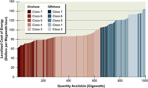
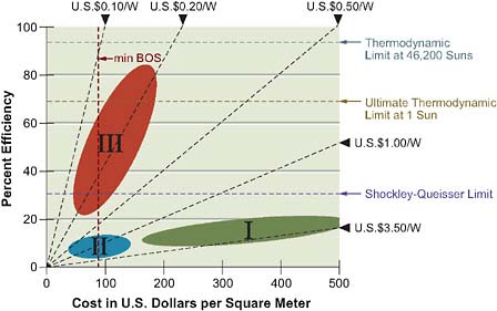
FIGURE 4.9 PV power costs as function of module efficiency and cost.
Source: Green, 2004. Copyright 2004 by Springer. Reprinted with permission of Springer Science+Business Media.
cost of a PV cell module is typically expressed as dollars per peak watt of production ($/Wp) and is determined by the ratio of the module cost per unit of area ($/m2) divided by the maximum amount of electric power delivered per unit of area (module efficiency multiplied by 1000 W/m2, the standard insolation rate at 25ºC). In Figure 4.9, this cost per peak watt is indicated by a series of dashed straight lines having different slopes. Any combination of area cost and efficiency on a given dashed line produces the same cost per peak watt indicated by the line labels. For example, present single-crystalline Si PV cells, with an efficiency of 10 percent and a cost of $350/m2, have a module cost of $3.50/Wp. The area labeled I in Figure 4.9 represents the first generation (Generation I) of solar cells and covers the range of module costs for these cells. Areas labeled II and III in Figure 4.9 present the target module costs for Generation II (thin-film PV) and Generation III PV cells (advanced future structures) that are still in development.
In addition to module costs, a PV system also has costs associated with the non-photoactive parts of the system, called balance of system (BOS) costs, which are in the range of $250/m2 for Generation I cells. The total cost of current PV systems is about $6/Wp. Taking into account the cost of capital, interest rates, depreciation, system lifetime, and the available annual solar irradiance integrated
over the year (i.e., considering the diurnal cycle and cloud cover, which reduce the peak power by a factor of about 1/5), the $/Wp figure of merit can be converted to $/kWh by the following simple relationship: $1/Wp ~ $0.05/kWh. This calculation leads to a present cost for grid-connected PV electricity of about $0.30/kWh. The estimates of levelized energy costs for PV generally are distributed around the 30¢/kWh level, as shown in Annex Table 4.A.2. The one exception was a 2004 SEIA study of levelized costs that predicted the cost of energy from PV would fall to about $0.14/kWh by 2010, in the absence of aggressive policies to promote the technology, and to $0.08/kWh with such policies in place.
The costs of supplying electricity from rooftop PV installations will vary across different locations and depend on factors such as the cost of land, options for orienting the installation (particularly on rooftops), and amount of energy produced in a particular location. A study of the factors affecting supply curves for solar PV from rooftops used data on building stock, rooftop orientation, solar insolation, and other factors to construct relative supply functions for solar PV for three U.S. electric interconnections as shown in Figure 4.10 (Denholm and Margolis, 2008). These supply curves relate to the system with the greatest yield, which results from the best orientation in the most productive location. The sup-
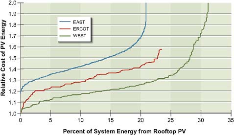
FIGURE 4.10 Fractional energy PV rooftop supply curves for three U.S. interconnections.
Source: Denholm and Margolis, 2008.
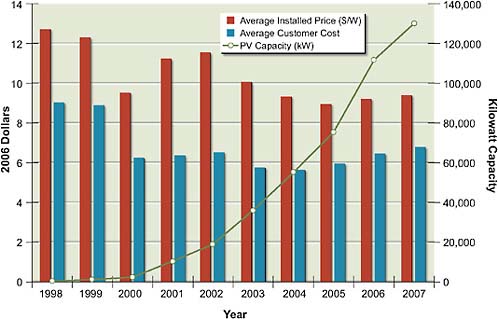
FIGURE 4.11 Price, customer cost after subsidy, and number of PV installations per year in California under California Energy Commission incentive programs.
Source: CEC, 2008.
ply curves show the higher costs of producing electricity using solar PV in the east compared to the west, and the resource limits in different locations.
Largely as a result of state-level policies to promote the use of solar PV, the number of installations is growing. As shown in Figure 4.11, in California about 130 MW of the cumulative PV capacity installed by 2007 was under incentive programs administered by the California Energy Commission (CEC), more than double the total amount installed under these programs as of 2004. This increase in capacity coincided with the 2006 launch of the California Solar Initiative with a funding level of about $3.3 billion for subsidy payments available to new solar PV installations. Data from the CEC on total costs and costs to customers of PV installations suggest that costs per kilowatt for consumers rose slightly over this period, a period of only slight increases in consumer costs per watt of PV installations, due in part to the subsidies afforded by the California policy (CEC, 2008). The CEC PV database contains information on about one-third of the total amount of PV capacity installed in California.
Most of the solar PV installations appear to be taking place in regions that have aggressive pro-solar policies. According to solarbuzz.com, in 2006 California accounted for 63 percent of the grid-connected PV market, and New Jersey, which also has an aggressive policy to promote PV, accounted for 19 percent. In general, achieving grid parity, the point at which electricity from PV is equal to or cheaper than power from the electricity grid, would require a two- to three-times improvement for costs per kilowatt-hour for the whole system (PV modules, batteries, inverters, and other system components) as well as for installation and O&M costs (Cornelius, 2007).
Concentrating Solar Power
According to the EIA (2008d) AEO 2009 model runs, the levelized cost of generating electricity using concentrating solar power (CSP) is higher than the cost with wind, but lower than the cost of solar PV as shown in Table 4.2. If technological learning for CSP is a function of aggregate investment, as assumed by the EIA, then the economics of CSP may be improved by policies that promote investment in this technology and provide incentives for using it to generate electricity. Twelve states have set-asides for solar technologies in their RPS policies, and in nine of those states, which include Arizona, New Mexico, and Nevada, solar thermal generating technologies for hot water generation qualify for the set-aside (Wiser and Barbose, 2008). The set-aside typically requires that a specific portion of the RPS target must be met with a solar technology. Some policies also include a credit multiplier for generation from solar such that solar-produced electricity creates RECs at a ratio of greater than 1:1.
Estimates of the levelized cost of central station CSP have typically been around 16¢/kWh at the busbar (Venkataraman et al., 2007; WGA, 2006b; EIA, 2008c). Table 4.2 shows that EIA reported a much higher levelized cost of 25¢/kWh in the AEO 2009 forecast, reflecting increases in 2007–2008 in raw materials costs (EIA, 2008d). With the 16¢ cost as a starting point, the supply curve for CSP in the southwestern United States shown in Figure 4.12 displays costs at the busbar. The total supply curve in this graph is the horizontal sum of the individual supply curves for different levels of solar resource intensity. This cost curve is very flat at levels of around 16¢/kWh.
Figure 4.13 shows a supply curve that goes beyond the busbar and takes into account the costs of incremental transmission necessary to deliver power to load. This curve is based on assumptions about the portion of local load that
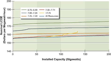
FIGURE 4.12 Supply curves describe the potential capacity and current busbar costs in terms of nominal levelized cost of energy (LCOE) of concentrating solar power. Colored lines indicate different amounts of insolation measured in kilowatt-hours per square meter per day.
Source: ASES, 2007. Used with permission of the American Solar Energy Society. Copyright 2007 ASES.
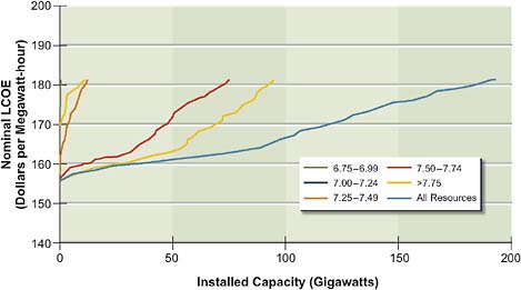
FIGURE 4.13 Concentrating solar power supply curve based on 20 percent availability of city peak demand and 20 percent availability of transmission capacity. Colored lines indicate different amounts of insolation measured in kilowatt-hours per square meter per day.
Source: ASES, 2007. Used with permission of the American Solar Energy Society. Copyright 2007 ASES.
could be served by solar power, the availability of transmission to move power from generation sites to load centers, and the cost of expanding transmission at $1000/MW-mile, lower than the $1600/MW-mile used in the DOE (2008) 20 percent wind study. As shown in Figure 4.13, the resulting aggregate supply curve for this region has a bit of slope to it, rising to approximately 18¢/kWh at or near 180 GW of generation. The basic message from the fairly flat slope of this supply curve is that at this time the constraining factor for concentrating solar power supply is not the amount of the resource, which is widely distributed and available abundantly in the southwest, but the costs of developing that resource.
How this cost picture might change over time depends on future adoption of renewable technologies. According to the WGA study, technology learning and economies of scale in manufacturing and installation indicate that the levelized cost of energy in 2015 for a parabolic trough technology would decrease by 50 percent with an increase of 4 GW of installed capacity (WGA, 2006b). The American Solar Energy Society (2007) anticipates further decreases in levelized cost of another 25 percent between 2015 and 2030. Research and development is also expected to have an important effect on costs. The DOE’s Office of EERE (NREL, 2007) anticipates that both capital costs and capacity factors for CSP could improve dramatically through its R&D program for concentrating solar power, including storage capacity and location of new systems in the most productive sites. Levelized costs of energy at the busbar could decrease by 50 percent as soon as 2010, as shown in Table 4.A.1, though this sounds quite optimistic.
Geothermal Power
Most of the economic U.S. hydrothermal resources are located in the western states. Recent studies sponsored by the WGA (WGA, 2006a) identify approximately 13,600 MW of geothermal potential in the west that could be developed economically, at busbar costs of up to 20¢/kWh in $2005, and 5,600 MW that reasonably could be developed by 2015 at costs of less than 10¢/kWh in $2005. Both cost estimates omit the renewable PTC that would reduce the costs of developing these resources.
The WGA report and one conducted by the CEC (GeothermEX Inc., 2004) were used to update the geothermal supply curves in NEMS (Smith, 2006). The supply curves are limited to the 80 most likely sites to be developed and extend to include 8 GW of new capacity. The NEMS geothermal supply curve, shown in Figure 4.14, is similar to the supply curves found in the WGA report. According
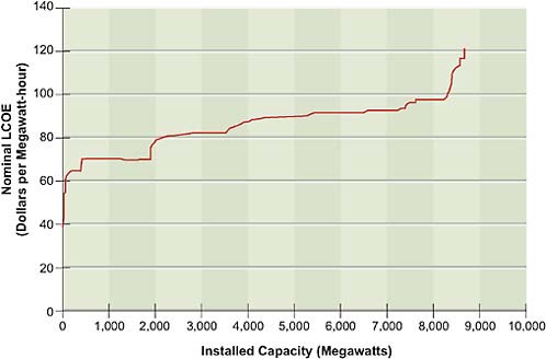
FIGURE 4.14 Geothermal supply curve.
Source: Developed from data supplied by Smith, 2006.
to EIA, this supply curve, added to the NEMS model with the development of AEO 2007, would not capture all potentially economic geothermal resources, but it is an important start and likely does capture the most economic resources available (Smith, 2006). Enhanced geothermal systems (EGS) may offer greater opportunity in the future, but, as indicated in Chapter 3, this technology is too early in its development to reliably estimate its cost.
Existing geothermal generating capacity is closer to 2.5 GW (EIA, 2008c). One hurdle to the development of geothermal resources is that, like wind, they may be located far from load and require new transmission lines to facilitate delivery. However, geothermal energy provides constant, baseload power, which is an advantage over solar and wind.
Biopower
The costs of new biopower generation will depend on two important factors: the generation technology and the cost of the fuel. In its NEMS model, EIA assumed
that any new biopower generation would use gasification with a combined cycle technology. These generators have high capital costs and lower heat rates than a conventional boiler. However, none of these types of biopower generators are now in commercial operation in the United States, so it is difficult to know how the predicted costs would compare to actual experience.19 In its Technology Assessment Guide, EPRI reported costs for both stoker and circulating fluidized bed boilers, technologies that are well suited to the small scale of most biomass plants and that can handle the fuel well EPRI (2007a). Capital costs, including interest during construction and project specific costs, would be on the order of $3400/kW for each technology with capacity factors of 85 percent. The levelized cost of energy would depend on fuel costs, but the EPRI summer study reports a cost of approximately 9.6¢/kWh for a fluidized bed generator in 2010, which, assuming similar fuel costs of $34/MWh (about $2.70/million Btu of high heat value), would yield a levelized cost estimate for a stoker of 9.4¢/kWh.20
The costs of biomass fuels are also subject to uncertainty and potential volatility. Much of the existing biopower generation occurs as self-generation at facilities that have a ready source of fuel (such as pulping operations, paper mills, or forest products plants). Expanding capabilities beyond these generators could involve shipping fuel, which can become quite costly, which suggests that future biopower generation capability would be located close to fuel sources and would use more economical biomass fuels that are concentrated locally and do not face substantial competition for their use.
This uncertainty about fuel costs is reflected in the different estimates of levelized costs of biopower reported in Annex Table 4.A.1. The fuel cost assumptions in the recent EIA forecasts are substantially lower than those assumed by other sources, including EPRI and S&P. These lower costs are a major factor in the substantially lower levelized cost of energy in the EIA numbers, which are about 85 percent lower than those provided by other sources.
One option for greater use of biomass fuel is co-firing the fuel with coal. Biomass co-firing of up to 10 to 15 percent of fuel on a heat-input basis is a potential way of reducing the CO2 emissions associated with coal-fired generation (NREL, 2006). The costs of making a coal-fired generation facility available for
|
19 |
NEMS includes this technology instead of biomass combustion in boilers under the expectation that gasification, once commercial, could trump biomass combustion and the need for the model to be somewhat parsimonious in including different technologies. |
|
20 |
See Table 4.A.1 for all the components of cost. |
co-firing could be substantial and involve large investments in new fuel-handling equipment. Certain types of boiler configurations are more amenable than others. Even though co-firing counts as renewable generation under many state RPS policies, co-firing has not increased much in response to state RPS policies (McElroy, 2008). Placing a cap on CO2 emissions may be necessary to drive coal plants to start making the investment necessary to co-fire, and then only when the facility can identify an economic source of biomass fuel.
COSTS IN 2020
Table 4.A.2 in the annex at the end of this chapter provides estimates from a few different sources of the levelized costs in 2020 of a range of different renewable technologies. These sources include the EIA AEO 2009 reference case forecast, the EERE Office at DOE, EPRI, the SEIA, U.S. DOE’s 20 percent wind study, and the cost estimates published in a 2007 report edited by the American Solar Energy Society. Table 4.A.2 also includes levelized cost of energy projections for a number of fossil generation technologies based on the AEO 2009 forecasts. These forecasts all include the effect of learning on reducing capital costs, where the potential cost reductions from learning vary across technologies. The projections from EIA also include the effect of moving along the supply curve, such as when less accessible or lower quality wind resources are tapped for wind electricity generation.
Table 4.A.2 shows a wide range of forecasts on the future of renewables costs. Most of the forecasts envision renewables as continuing to be more costly than the EIA forecasts of generation using conventional coal and gas technologies. The exceptions are the EERE forecasts that envision substantial improvements in costs for concentrating solar power and wind, and the SEIA forecast for solar PV. The differences between the program scenarios and the baseline scenarios for the EERE forecasts show how full funding of renewable energy research at DOE is expected to affect the future costs of renewable generation.
The different forecasting groups and scenarios also envision different rates of change in levelized costs of energy over the next decade as shown in Figure 4.15, which compares forecasts of costs for 2020 and 2010 for several sources for four of the technologies. This graph shows that EERE and EPRI summer study forecasts envision large decreases in the costs of wind generation between 2010 and 2020, whereas the levelized costs in EIA forecasts increase as a result of the cost
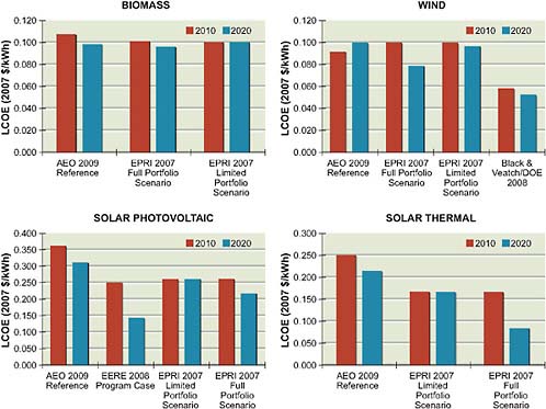
FIGURE 4.15 Levelized cost of energy for selected renewable technologies in 2010 and 2020 from various sources. Note that AEO 2009 numbers are for 2012.
increases inherent in tapping increasingly difficult sites, which are not reflected in the estimates reported by the other studies.
Differences in cost projections for wind turbines appear to be at least partly due to differences in assumptions about capacity factors. The predictions from EERE are largely the result of improvements in engineering resulting from research and development in this technology and greater deployment. In the AEO projections, capacity factor predictions for 2020 are based on where the wind resource would be developed in that year. The model presumably would have used up the better sites for the least-cost development of resources in earlier years. Incorporating resources found in higher wind class regions, as suggested in Figure 4.7, would
likely lead to lower capacity factors at new facilities after the better wind sites are taken.
The DOE 20 percent wind study assumed that, as a result of technology improvements, capacity factors would improve between 2005 and 2030 by 10–18.7 percent, with faster rates of improvement anticipated in the lower wind resource regions (DOE, 2008). Most of this improvement is expected by 2020. This study also assumed that capital costs of new onshore wind generators would fall by 5 percent between 2005 and 2020, and that new offshore wind generators would see capital cost decreases of just over 10 percent during the same period. This study also anticipated a marked decline in variable and fixed O&M costs between 2005 and 2020, particularly for offshore installations.
CSP and PV also have a wide range of future cost predictions, representing the large degree of uncertainty and differing opinions about how solar costs are likely to evolve over this decade. PV is expected to remain more expensive than CSP, although the SEIA forecasts dramatic improvement in the cost of distributed PV, and EERE anticipates decreases in PV costs, too. EERE also projects potential cost improvements for solar thermal projects. But unlike other forecasters, EERE predicts substantially lower costs in the near term, suggesting differences in what goes into their cost measures. The DOE Solar Energy Technologies Program report envisions declines in CSP costs of about 50 percent from present levels, similar to the aggressive technology case from the EPRI summer study.
Analysis of the evolution of PV costs suggests that the prices of PV modules have followed a historical trend along the “80 percent learning curve.” That is, for every doubling of the total cumulative production of PV modules worldwide, the price has dropped by approximately 20 percent. This trend is illustrated in Figure 4.16 (Surek, 2005). The final data point for 2003 corresponds to about $3.50/Wp and a cumulative PV capacity of 3 GW. A major reduction in the projected future cost of PV modules depends on the introduction of thin films, concentrator systems, and new technologies. The graph projects the path of future costs under historical learning rates as well as with slower and faster rates of learning.
ANALYSIS OF 2020 COST PROJECTIONS
Cost projections for renewables can vary widely within a particular resource type and technology, depending on the source and the assumptions. For this report, the panel did not have access to all of the underlying assumptions, ren-
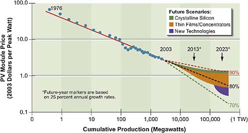
FIGURE 4.16 Learning curve for PV production.
Source: Surek, 2005.
dering impossible a total breakdown of the differences among different sources. The panel did have sufficient information to compare the assumptions and the general approaches to developing projections of costs and to make substantive comments.
The panel is aware of the difficulties of predicting future energy prices, especially after observing the cost of a barrel of light crude oil vary from a low of $35 per barrel to a high of almost $140 per barrel within the span of 12 months. Such volatilities should humble any group attempting to predict the future. The panel considers these alternate cost estimates to come from reputable sources and to be representative of the range of cost estimates for renewables in the future. Taking all of these factors into consideration, the panel supported the idea that the upper cost bounds in these estimates are in line with the panel’s estimate of a reasonable upper bound, while some of the lower cost estimates tended to represent aspirational goals. Volatilities in energy and commodities markets and other large-scale macroeconomic factors are difficult to predict, and therefore the panel does not label any projection as more correct than another.
Nevertheless, the panel considers it essential to understand why these estimates vary. Indeed, while the most recent AEO 2009 shows a significant increase in PV costs over AEO 2008 (see Table 4.2), recent reports indicate a drastic
decrease in solar PV due to increased supply and decreased demand (Patel, 2009). One key factor is the assumed cost of capital equipment today, and whether or not it reflects recent increases in costs for material and labor, wind turbines, solar panel components, and construction in general. Material and construction cost increases in the past few years have resulted in substantially higher costs of new facilities and have tended to more than offset reductions in capital costs for wind turbines and solar PV installations from technology learning over that short time horizon. Some studies, such as the DOE 20 percent wind penetration study and AEO 2009, more fully reflect these recent cost increases, while others, including EERE, only partially inflate the costs, possibly in trying to capture just the portion of the recent cost increases anticipated to be long-lived, rather than short-run spikes in costs that will likely be resolved over time.
Assumptions about technology learning and its likely evolution independent of scale of deployment are also key to projections about future costs. The EIA NEMS model assumes that substantial cost reductions will occur over time for CSP and solar PV technologies as a result of learning both from greater deployment and from research and development. The model assumes high initial learning rates, with initial capital costs projected to decrease by at least 20 percent by 2025, and potentially more if the technology is widely adopted. The NEMS model also assumes that gasification technology forecasted for new biopower installations will realize substantial cost reductions as installations of this technology, either for use with coal or biomass, grow. On the other hand, the model treats wind as a fairly mature technology and assumes fairly low rates of improvement in costs in the future, with a 1 percent reduction in capital costs for each doubling of installed capacity.
These different learning assumptions help explain the differences in cost improvements over time among the different technologies within the EIA projections. The fact that other studies, such as the DOE (2008) 20 percent wind study, are more bullish on the possibility of improvements in cost of wind technology explains some of the differences in projections of levelized costs across studies. The 20 percent wind study also assumes larger improvements in capacity factors of wind turbines over time than the maximum potential improvements in performance allowed in the NEMS model. These differences in assumptions contribute to differences in the projections of future levelized costs.
For studies that assume technology learning is a function of the level of installed capacity, the underlying assumptions about policies to promote renew-
ables and how those policies and market dynamics will play out in the future renewables market will affect projections of the LCOE. The approach to modeling state-level RPS policies and assumptions about the future of the PTC will influence the predictions of future costs, and possibly performance, of renewables. For AEO 2009, assumptions include regional compliance with relevant state RPS requirements and expiration of the PTC at the end of 2009 for wind and 2010 for other technologies. Changes in these policies will affect gains from capacity-related learning. For example, the recent extension of the PTC beyond the 2009 or 2010 expiration dates could increase learning-related improvements in costs. On the other hand, substantial increases in investment in energy efficiency and associated reductions in electricity demand could lower projected renewables penetrations by 2020 and reduce the gains from capacity-related learning. The DOE (2008) 20 percent wind study imposes only external assumptions about technology learning that are a function of time, but not of overall penetration, and so the level of penetration before 2020 does not matter for learning, but it does matter for determining where each region will find itself in 2020 on the relevant wind supply curves.
In general, projections that are more in the form of goals for renewable technology performance tend to be more optimistic than projections based on learning, whether the learning is from projections of past trends or as a function of anticipated deployment, which is in turn determined partly based on policy assumptions. Thus, the SEIA and EERE projections for the costs of solar technologies tend to be more optimistic than those from other sources.
Cost projections for biopower depend on the assumed technology. For its NEMS model projections, EIA assumes that all new investment in biopower will use an integrated gasification combined cycle (IGCC) technology that has a very low heat rate and relatively low capital costs, whereas EPRI, in its 2007 summer study, assumes that new biopower is generated using a stoker boiler technology that has somewhat higher capital costs and a much higher heat rate. The comparability of these two cost assumptions is unclear, given the complexity of the IGCC technology relative to the proven stoker boiler technology. The fact that biopower from IGCC technology is a relatively untested technology in the United States at this time is also not reflected in these different estimates, and thus the cost estimates from EIA are based on engineering projections and not on actual experience with the technology.
FINDINGS
The most critical elements of the panel’s findings on the economics of renewable electricity generation are highlighted below.
A principal barrier to the widespread adoption of renewable electricity technologies is that electricity from renewables (except for electricity from large-scale hydropower) is more costly to produce than electricity from fossil fuels without an internalization of the costs of carbon emissions and other potential societal impacts. Policy incentives, such as renewables portfolio standards, the production tax credit, feed-in tariffs, and greenhouse gas controls, thus have been required, and for the foreseeable future will continue to be required, to drive further increases in the use of renewable sources of electricity.
Unlike some conventional energy resources, renewable electricity is considered manufactured energy, meaning that the largest proportion of costs, external energy, and materials inputs, as well as environmental impacts, occur during manufacturing and deployment rather than during operation. In general, the use of renewable resources for electricity generation involves trading the risks of future cost increases for fossil fuels and uncertainties over future costs of carbon controls for present fixed capital costs that typically are higher for use of renewable resources than for use of fossil fuels. Except for biopower, no fuel costs are associated with renewable electricity sources. Further, in contrast to coal and nuclear electricity plants, in which larger facilities tend to exhibit lower average costs of generation than do smaller plants, for renewable electricity the opportunities for achieving economies of scale are generally greater at the equipment manufacturing stage than at the generating site itself.
The future evolution of costs for generation of electricity from renewable resources will depend on continued technological progress and breakthroughs. It will also depend on the potential for policies to create greater penetration and to accelerate the scale of production largely an issue of long-term policy stability and policy clarity. Markets will generally exploit the lowest-cost resource options first, and thus the costs of renewables may not decline in a smooth trajectory over time. For example, in the case of wind power, the lowest-cost resources are generally available at the most accessible sites in the highest wind class areas. Development of these prime resources will thus entail significant resource cost shifts as markets adjust to exploit next-tier resources. At present, onshore wind is an economically favored option relative to other (non-hydroelectric) renewable resources, and
hence wind power is expected to continue to grow rapidly if recent policy initiatives continue into the future.
Although some forecasts show that biopower will play an important role in meeting future RPS targets, the degree of competition with and recent mandates for use of liquid biofuels for providing transportation fuel and, of course, the use of biomass for food, agricultural feed, and other uses will impact the prospects for greater use of biomass in the electricity market. The future of distributed renewable electricity generation from sources such as residential photovoltaics will depend on how its costs compare to the retail price of power delivered to end users, on whether prices fully reflect variations in cost over the course of the day, and on whether the external costs of fossil-based electricity generation are increasingly incorporated into its price.
Formulation of robust predictions about whether the price of electricity will meet or exceed the price required for renewable sources to be profitable and what their resulting level of market penetration will be remain a difficult proposition. Comparisons between past forecasts of renewable electricity penetration and actual data show that, while renewable technologies generally have met forecasts of cost reductions, they have fallen short of deployment projections. Further, the profitability and penetration of electricity generated from renewable resources may be sensitive to investments in energy efficiency, especially if efficiency improvements are sufficient to meet growth in the demand for electricity or to lower the market-clearing price of electricity. If the financial operating environment for fossil-fuel and other in-place sources of electricity remains unchanged, then the competitiveness of renewable electricity may be affected more than that of other electricity sources. However, at this time, the deployment of renewable electricity is being driven by tax policies, in particular by the renewable production tax credit, and by renewable portfolio standards.
In particular, the panel finds that:
-
Onshore wind is an economic option that could scale to a material penetration by 2020, and will likely see rapid growth if recent policy initiatives continue into the future. Biopower is also forecast to play an important role in meeting future RPS targets, but greater use in the future electricity market will depend on competition from demand for liquid biofuels for transportation.
-
Some kind of incentive (RPS with high REC price, PTC, or feed-in tariff) will be needed to increase renewables’ use as long as external costs
-
of fossil generation, particularly those associated with greenhouse gas emissions, are not incorporated into the costs of using those technologies and fuels.
-
Renewables policies will be more effective if they are stable and predictable than if they cycle on and off or have a highly uncertain future, as has been the case with the federal PTC.
-
Intermittency of wind is manageable using current technology, and storage is not required for levels of market penetration expected within the 2020 timeframe.
-
The evolution of renewables’ costs will depend on technological breakthroughs, the potential for policies to achieve greater market penetration and technological learning, and the rapidity with which low-cost resources, such as the most accessible sites in the highest wind class areas, are exhausted.
-
Investment in energy efficiency, which can lower the market-clearing price of electricity, could diminish the future profitability of renewable electricity generation.
-
A key determinant of the future success of renewables in penetrating the market is the value that renewables suppliers will obtain for their generation in the electricity marketplace, which is largely determined by the wholesale market price of electricity for grid-scale renewables and the retail price of electricity for distributed renewables. Predicting that price and the resulting level of renewables market penetration has been and continues to be a difficult proposition.
-
Projections of levelized costs of energy in 2020 for wind across all data sources are generally no higher than EIA projections of levelized costs for coal integrated gasification combined cycle with carbon capture and storage or natural gas combined cycle with carbon capture and storage. However, the full costs of integrating wind power into the grid, which are not typically reflected in levelized cost projections, could lead to a change in the relative cost ranking of these technologies.
REFERENCES
ASES (American Solar Energy Society). 2007. Tackling Climate Change in the U.S.: Potential Carbon Emission Reductions from Energy Efficiency and Renewable Energy by 2030. Washington, D.C.
Bierden, P. 2007. The process of developing wind power generators. Presentation at the second meeting of the Panel on Electricity from Renewable Resources, December 6, 2007. Washington, D.C.
Bird, L., and B. Swezey. 2006. Green Power Marketing in the United States: A Status Report. 9th Edition. NREL/TP-640-40904. Golden, Colo.: National Renewable Energy Laboratory. November.
Bird, L., and E. Lockey. 2007. Interaction of Compliance and Voluntary Renewable Energy Markets. NREL/TP-670-42096. Golden, Colo.: National Renewable Energy Laboratory. October.
Bird, L., L. Dagler, and B. Swezey. 2007. Green Power Marketing in the United States: A Status Report. 10th Edition. NREL/TP-670-42502. Golden, Colo.: National Renewable Energy Laboratory. December.
Black & Veatch. 2007. 20 Percent Wind Energy Penetration in the United States—A Technical Analysis of the Energy Resource. Black & Veatch Project #144864, prepared for the American Wind Energy Association, Walnut Creek, Calif.
Borenstein, S. 2007. Electricity Rate Structures and the Economics of Solar PV: Could Mandatory Time-of-Use Rates Undermine California’s Solar Photovoltaic Subsidies? Center for the Study of Energy Markets Working Paper 172. University of California, Berkeley. September. Available at http://www.ucei.berkeley.edu/PDF/csemwp172.pdf.
Borenstein, S. 2008a. The Market Value and Cost of Solar Photovoltaic Electricity Production. Center for the Study of Energy Markets Working Paper 176. University of California, Berkeley. January.
Borenstein, S. 2008b. Response to Critics of “The Market Value and Cost of Solar Photovoltaic Electricity Production.” Available at http://faculty.haas.berkeley.edu/borenste/SolarResponse.pdf.
CEC (California Energy Commission). 2008. Energy Renewable Programs. Available at http://www.energy.ca.gov/renewables/emerging_renewables/index.html.
Cornelius, C. 2007. DOE Solar Energy Technologies Program. Presentation at the first meeting of the Panel on Electricity from Renewable Resources, September 18, 2007. Washington, D.C.
Cory, K.S., and B.G. Swezey. 2007. Renewable Portfolio Standards in the States: Balancing Goals and Implementation Strategies. Technical Report NREL/TP- 670-41409. Golden, Colo.: National Renewable Energy Laboratory. December.
DeCarolis, J.F., and D.W. Keith. 2004. The economics of large-scale wind power in a carbon constrained world. Energy Policy 34:395-410.
Denholm, P., and R. Margolis. 2008. Supply Curves for Rooftop Solar PV-Generated Electricity for the United States. Technical Report, NREL/TP-6A0-44073. Golden, Colo.: National Renewable Energy Laboratory. November.
DOE (U.S. Department of Energy). 2008. 20% Wind Energy by 2030: Increasing Wind Energy’s Contribution to U.S. Electricity Supply. Office of Energy Efficiency and Renewable Energy. Washington, D.C.: U.S. DOE.
Economist. 2008. German lessons: An ambitious cross-subsidy scheme has given rise to a new industry. Vol. 387(8574), pp. 67-68, April 5.
EIA (Energy Information Administration). 2004. Analysis of S. 1844, the Clear Skies Act of 2003; S. 843, the Clean Air Planning Act of 2003; and S. 366, the Clean Power Act of 2003. SR/OIAF/2004-05. Washington, D.C.: U.S. Department of Energy, EIA. May.
EIA. 2005. Production Tax Credit for Renewable Energy Generation, Issues in Focus, AEO2005. Washington, D.C.: U.S. Department of Energy, EIA.
EIA. 2007a. Assumptions to the Annual Energy Outlook for 2007. DOE/EIA-0554(2007). Washington, D.C.: U.S. Department of Energy, EIA.
EIA. 2007b. Analysis of Alternative Extensions of the Existing Production Tax Credit for Wind Generators. Memorandum to the Committee on Ways and Means, U.S. House of Representatives. Washington, D.C.: U.S. Department of Energy, EIA.
EIA. 2007c. Impacts of a 15-Percent Renewable Portfolio Standard. SR/OIAF/2007-03. Washington, D.C.: U.S. Department of Energy, EIA.
EIA. 2008a. Energy Market and Economic Impacts of S. 1766, The Low Carbon Economy Act of 2007. SR/OIAF/2007-06. Washington, D.C.: U.S. Department of Energy, EIA.
EIA. 2008b. Energy and Economic Impacts of Implementing Both a 25-Percent Renewable Portfolio Standard and a 25-Percent Renewable Fuel Standard by 2025. SR/ OIAF/2007-05. Washington, D.C.: U.S. Department of Energy, EIA.
EIA. 2008c. Annual Energy Outlook 2008 with Projections to 2030. DOE/EIA-0383(2008). Washington, D.C.: U.S. Department of Energy, EIA.
EIA. 2008d. Annual Energy Outlook 2009, Early Release. DOE/EIA-0383(2009). Washington, D.C.: U.S. Department of Energy, EIA.
EPA (U.S. Environmental Protection Agency). 2008. EPA Analysis of the Lieberman-Warner Climate Security Act of 2008, S. 2191 in the 110th Congress. Washington, D.C.
EPRI (Electric Power Research Institute). 2007a. Renewable Energy Technical Assessment Guide. Palo Alto, Calif.
EPRI. 2007b. The Power to Reduce CO2 Emissions: The Full Portfolio. Palo Alto, Calif.
ERCOT (Electric Reliability Counsel of Texas). 2007. ERCOT Target Reserve Margin Analysis. Sacramento, Calif.: Global Energy Decisions, Inc.
EWEA (European Wind Energy Association). 2005. Large Scale Integration of Wind Energy in the European Power Supply: Analysis, Issues and Recommendations. Brussels.
FERC (Federal Energy Regulatory Commission). 2006. Assessment of Demand Response and Advanced Metering Staff Report. Docket AD06-2-000. Washington, D.C.
GE Energy Consulting. 2005. The Effects of Integrating Wind Power on Transmission System Planning, Reliability, and Operations. Prepared for New York State Energy Research and Development Authority, Albany, N.Y.
GeothermEx, Inc. 2004. New Geothermal Site Identification and Qualification. Report to the California Energy Commission, Public Interest Energy Research Program, Sacramento, Calif.
German Federal Ministry for the Environment, Nature Conservation, and Nuclear Safety. 2007. Renewable Energy Sources in Figures—National and International Development. Bonn, Germany.
Green, M.A. 2004. Third Generation Photovoltaics: Advanced Solar Energy Conversion. Berlin: Springer.
Harper, J.P., M.D. Karcher, and M. Bolinger. 2007. Wind Project Financing Structures: A Review and Comparative Analysis. Technical Report LBNL-63434. Berkeley, Calif.: Lawrence Berkeley National Laboratory. September.
IEA (International Energy Agency). 2006. Renewables Database. Renewable Energy Feed-in Tariffs (III). Paris. Available at http://www.iea.org/textbase/pm/?mode=re&id=3846&action=detail.
Klein, A., A. Held, M. Ragwitz, G. Resch, and T. Faber. 2006. Evaluation of Different Feed-In Tariff Design Options—Best Practice for the International Feed-In Cooperation. Fraunhofer Institute Systems and Innovation Research, Economics Group, Karlsruhe, Germany.
McElroy, A.K. 2008. Lukewarm on co-firing. Biomass Magazine. February. Available at http://www.biomassmagazine.com/article.jsp?article_id=1429&q=&page=all.
McVeigh, J., D. Burtraw, J. Darmstadter, and K. Palmer. 2000. Winner, loser, or innocent victim: Has renewable energy performed as expected? Solar Energy 68(3):237-255.
Mills, A., and R. Wiser. 2009. The Cost of Transmission for Wind Energy: A Review of Transmission Planning Studies. Berkeley, Calif.: Lawrence Berkeley National Laboratory.
NREL (National Renewable Energy Laboratory). 2006. Power Technologies Energy Data Book. NREL/TP-620-39728. Golden, Colo. August. Available at http://www.nrel.gov/analysis/power_databook/.
NREL. 2007. Projected Benefits of Federal Energy Efficiency and Renewable Energy Programs. NREL/TP-640-41347. Golden, Colo. March. Available at http://www1.eere.energy.gov/ba/pba/pdfs/41347.pdf.
Palmer, K., and D. Burtraw. 2005. Cost effectiveness of renewable energy policies. Energy Economics 27:873-894.
Palmer, K., D. Burtraw, and J.S. Shih. 2007. The benefits and costs of reducing emissions from the electricity sector. Journal of Environmental Management 83:1.
Patel, S. 2009. PV sales in the U.S. soar as solar panel prices plummet. Power Magazine, March 1.
Rastler, D. 2008. Electric energy storage briefing. Presentation at the fourth meeting of the Panel on Electricity from Renewable Resources, March 11, 2008. Washington, D.C.
Ridge Energy Storage and Grid Services, L.P. 2005. The Economic Impact of CAES of Wind in TX, OK, and NM. Final Report for Texas State Energy Conservation Office, Austin, Tex. June 27.
Royal Academy of Engineering. 2004. The Costs of Generating Electricity. London.
SEIA (Solar Energy Industries Association). 2004. Our Solar Power Future—The U.S. Photovoltaic Industry Roadmap Through 2030 and Beyond. Washington, D.C.
Sheehan, G., and S. Hetznecker. 2008. Utility Scale Solar Power. IEEE Power & Energy Magazine 5 (October).
Short, W., and P. Denholm. 2006. A Preliminary Assessment of Plug-in Hybrid Electric Vehicles on Wind Energy Markets. NREL Technical Report. Golden, Colo.: National Renewable Energy Laboratory. April.
Smith, J.C. 2007. Integrating wind into the grid. Presentation to the America’s Energy Future Panel on Electricity from Renewable Resources, Washington, D.C. December 7.
Smith, R.K. 2006. EIA geothermal supply curve. Memorandum. Washington, D.C.: U.S. Department of Energy, EIA. September 15.
Surek, T. 2005. Crystal growth and materials research in photovoltaics: Progress and challenges. Journal of Crystal Growth 275:292-304.
Swezey, B., J. Aabakken, and L. Bird. 2007. A Preliminary Examination of the Supply and Demand Balance for Renewable Electricity. NREL/TP-670-42266. Golden, Colo.: National Renewable Energy Laboratory. October.
Vajjhala, S., A. Paul, R. Sweeney, and K. Palmer. 2008. Green corridors: Linking interregional transmission expansion and renewable energy policies. Discussion Paper 08-06. Washington, D.C.: Resources for the Future, Inc. March.
Venkataraman, S., D. Nikas, and T. Pratt. 2007. Which power generation technologies will take the lead in response to carbon controls? S&P Credit Research. New York: Standard and Poor’s. May 11.
WGA (Western Governors’ Association). 2006a. Clean and Diversified Energy Initiative: Geothermal Task Force Report. Denver, Colo.
WGA. 2006b. Clean and Diversified Energy Initiative: Solar Task Force Report. Denver, Colo.
Wiser, R. 2008. The development, deployment, and policy context of renewable electricity: A focus on wind. Presentation at the fourth meeting of the Panel on Electricity from Renewable Resources, March 11, 2008. Washington, D.C.
Wiser, R., and G. Barbose. 2008. Renewables Portfolio Standards in the United States: A Status Report with Data Through 2007. Berkeley, Calif.: Lawrence Berkeley National Laboratory.
Wiser, R., and M. Bolinger. 2008. Annual Report on U.S. Wind Power Installation, Cost and Performance Trends: 2007. DOE/GO-102008-2590. Washington, D.C.: U.S. Department of Energy.
ANNEX
TABLE 4.A.1 Current Cost Assumptions for Renewable Technologies (in 2007 Dollars)
|
Technology |
Source |
Case/Scenario |
Overnight Capital Cost ($/kW)a |
|
Biopower |
|
|
|
|
Biopower–IGCC |
EIA (2008d) |
Input table |
3766 |
|
Biopower–Stoker |
EPRI (2007a) |
3520 |
|
|
Biopower–50 MW fluidized bed |
EPRI (2007a) |
|
3629 |
|
Biopower |
Venkataraman et al. (2007) |
|
2596 |
|
Concentrating Solar Power |
|
|
|
|
Concentrating solar |
NREL (2007) |
Program |
3645 |
|
Concentrating solar |
EIA (2008d) |
Reference |
5021 |
|
Concentrating solar |
EPRI (2007b) |
Limited and full portfolio |
|
|
Concentrating solar–trough |
EPRI (2007a) |
|
3271 |
|
Concentrating solar |
Venkataraman et al. (2007) |
|
4153 |
|
Concentrating solar–trough |
ASES (2007) |
|
|
|
Photovoltaic |
|
|
|
|
Photovoltaic |
NREL (2007) |
Program |
4050 |
|
Photovoltaic–distributed |
EPRI (2007b) |
Limited and full portfolio |
|
|
Photovoltaic flat plate |
EPRI (2007a) |
|
5487 |
|
Photovoltaic 2-axis |
EPRI (2007a) |
|
8876 |
|
Photovoltaic–distributed |
SEIA (2004) |
Baseline |
|
|
Photovoltaic–distributed |
SEIA (2004) |
Roadmap |
|
|
Photovoltaic–central |
EIA (2008d) |
Input table |
6038 |
|
Capacity Factor (%) |
Variable O&M (+ Fuel Costs ) ($/MWh) |
Fixed O&M ($/kW) |
|
|
83 |
6.71 (+ $15)d |
64.45 |
0.080 |
|
85 |
3.74 (+ $35)e |
91.79 |
|
|
85 |
4.26 (+ $35)e |
94.49 |
|
|
85 |
7.27 (+ $28)e |
166.13 |
0.090 |
|
65 |
8.10 |
0.00 |
0.071g |
|
31 |
0.00 |
56.7 |
0.200 |
|
34 |
|
|
0.170 |
|
34 |
0.00 |
60.2f |
0.130 |
|
43 |
31.20 |
34.3 |
0.170 |
|
|
|
|
0.160–0.190 |
|
21 |
0.00 |
10.4 |
0.220g |
|
|
|
|
0.260 |
|
25 |
0.00 |
19.5 |
|
|
32 |
0.00 |
46.6 |
|
|
|
|
|
0.150 |
|
|
|
|
0.080 |
|
22 |
0.00 |
11.7 |
0.320 |
|
Technology |
Source |
Case/Scenario |
Overnight Capital Cost ($/kW)a |
|
Wind |
|
|
|
|
Onshore wind |
EIA (2008d) |
Input table |
1923 |
|
Onshore wind |
NREL (2007) |
Baseline |
1052 |
|
Onshore wind |
NREL (2007) |
Program |
927 |
|
Onshore wind |
EPRI (2007b) |
Limited and full portfolio |
|
|
Onshore wind |
EPRI (2007a) |
Class 6, 100 MW |
1820 |
|
Onshore wind |
Venkataraman et al. (2007) |
|
1765 |
|
Onshore wind |
Black & Veatch (2007) |
20% wind energy study |
1713 |
|
Onshore wind |
Midwest ISO |
MTEP 2008 reference |
1983 |
|
Offshore wind |
EIA (2008d) |
Input table |
3851 |
|
Offshore wind |
Black & Veatch (2007) |
20% wind energy study |
2388 |
|
Conventional |
|
|
|
|
Pulverized coal |
EIA (2008d) |
Input table |
2058 |
|
Conventional gas combined cycle |
EIA (2008d) |
Input table |
962 |
|
Conventional combustion turbine |
EIA (2008d) |
Input table |
670 |
|
a Fuel cost per megawatt-hour reported by source. b Calculated from inputs based on a 20-year economic life and real cost of capital of 7.5 percent. c Levelized costs here are generic and do not include site-specific development costs or cost of facilitating delivery. d Fuel cost imputed from AEO 2009 Early Release model solution. AEO 2009 Energy Prices (2007$/million Btu) in 2012 are $1.91 for coal, $6.63 for natural gas, and $1.96 for biomass. e Fuel cost per megawatt-hour imputed from EPRI summer study levelized cost and TAG specifications for CFB biomass plant. f This estimate comes from a personal communication with Steve Gehl of EPRI. g EERE numbers are for 2010. h Depending on wind class. |
|||
|
Capacity Factor (%) |
Variable O&M (+ Fuel Costs ) ($/MWh) |
Fixed O&M ($/kW) |
|
|
36 |
0.00 |
30.3 |
0.069c |
|
45 |
0.00 |
26.2 |
0.033g |
|
46 |
0.00 |
25.3 |
0.029g |
|
32.5 |
|
|
0.100 |
|
42 |
0.00 |
72.7 |
|
|
33 |
0.00 |
26.0 |
0.073c |
|
35–50h |
5.70 |
11.9 |
|
|
34 |
0.00 |
16.5 |
0.071c |
|
34 |
0.00 |
89.5 |
0.157c |
|
37–52h |
15.60 |
18.7 |
|
|
85 |
4.64 (+ $16.7)d |
27.53 |
0.050 |
|
87 |
2.09 (+ $45.1)d |
12.48 |
0.060 |
|
30 |
3.60 (+ $69.3)d |
12.11 |
0.100 |
TABLE 4.A.2 2020 Cost Projections and Comparisons (in 2007 Dollars)
|
Technology |
Source |
Case/Scenario |
Overnight Cost (/kW)a |
Capacity Factor (%) |
|
Conventional Sources |
|
|
|
|
|
Pulverized coal |
EIA (2008d) |
Reference |
1985 |
85 |
|
IGCC |
EIA (2008d) |
Reference |
2233 |
85 |
|
IGCC with sequestration |
EIA (2008d) |
Reference |
3171 |
85 |
|
Combined cycle |
EIA (2008d) |
Reference |
928 |
87 |
|
Advanced combined cycle |
EIA (2008d) |
Reference |
892 |
87 |
|
Advanced combined cycle with sequestration |
EIA (2008d) |
Reference |
1729 |
87 |
|
Combustion turbine |
EIA (2008d) |
Reference |
647 |
30 |
|
Advanced combustion turbine |
EIA (2008d) |
Reference |
587 |
30 |
|
Renewables |
|
|
|
|
|
Biopower |
|
|
|
|
|
Biopower |
EIA (2008d) |
Reference |
3390 |
83 |
|
Biopower–Stoker |
EPRI (2007b) |
Full portfolio |
|
85 |
|
Biopower–Stoker |
EPRI (2007b) |
Limited portfolio |
|
85 |
|
Biopower |
ASES (2007) |
WGA Biomass Task Force |
|
90 |
|
Geothermal |
|
|
|
|
|
Geothermal |
EIA (2008d) |
Reference |
1585 |
90 |
|
Concentrating Solar |
|
|
|
|
|
Concentrating solar |
NREL (2007) |
Program case |
2860 |
72 |
|
Concentrating solar |
EIA (2008d) |
Reference |
4130 |
31 |
|
Concentrating solar |
EPRI (2007b) |
Limited portfolio |
|
34 |
|
Concentrating solar |
EPRI (2007b) |
Full portfolio |
|
34 |
|
Photovoltaic |
|
|
|
|
|
Photovoltaic |
NREL (2007) |
Program |
2547 |
21 |
|
Photovoltaic |
EPRI (2007b) |
Full portfolio |
|
|
|
Photovoltaic |
EPRI (2007b) |
Limited portfolio |
|
|
|
Levelized Cost ($/kW) |
Total Capital Cost ($/MWh) |
Variable O&M/Fuel Costs ($/MWh) |
Fixed O&M ($/MWh) |
Transmission Cost ($/MWh) |
Levelized Cost of Energy ($/kWh)b |
|
195 |
52.30 |
23.06 |
3.70 |
3.61 |
0.083 [0.079] |
|
219 |
60.64 |
18.59 |
5.19 |
3.61 |
0.088 [0.084] |
|
311 |
69.54 |
23.26 |
6.19 |
4.01 |
0.103 [0.099] |
|
91 |
18.63 |
59.21 |
1.64 |
3.88 |
0.083 [0.079] |
|
88 |
17.98 |
55.46 |
1.54 |
3.88 |
0.079 [0.075] |
|
170 |
34.64 |
68.84 |
2.61 |
3.93 |
0.110 [0.106] |
|
63 |
33.55 |
88.49 |
4.61 |
11.41 |
0.138 [0.127] |
|
58 |
30.71 |
75.21 |
4.01 |
11.41 |
0.121 [0.110] |
|
333 |
61.62 |
22.81 |
8.86 |
4.14 |
0.097 [0.093] 0.096 0.101 ~0.080c |
|
156 |
75.44 |
0.00 |
22.22 |
5.00 |
0.103 [0.098] |
|
|
4.47 |
0.00 |
|
|
0.050 |
|
405 |
180.02 |
0.00 |
21.30 |
11.00 |
0.212 [0.201] 0.170 <0.083c |
|
250 |
135.81 |
0.00 |
5.59 |
|
0.141 0.220 0.260 |
|
Technology |
Source |
Case/Scenario |
Overnight Cost (/kW)a |
Capacity Factor (%) |
|
Photovoltaic |
EIA (2008d) |
Reference |
5185 |
22 |
|
Photovoltaic–distributed |
SEIA (2004) |
Baseline |
|
|
|
Photovoltaic–distributed |
SEIA (2004) |
Roadmap |
|
|
|
Photovoltaic–distributed |
ACES (2007) |
DOE’s Solar America Initiative |
2.50/Wp installed cost |
|
|
Wind |
|
|
|
|
|
Onshore wind |
EIA (2008d) |
Reference |
1896 |
35 |
|
Onshore wind |
NREL (2007) |
Program |
916 |
49 |
|
Onshore wind |
NREL (2007) |
Baseline |
1076 |
46 |
|
Onshore wind |
EPRI (2007b) |
Full portfolio |
|
42 |
|
Onshore wind |
EPRI (2007b) |
Limited portfolio |
|
33 |
|
Onshore wind |
Black & Veatch (2007); DOE (2008) |
DOE 20% wind study |
1630 |
38–52 (depending on wind class) |
|
Offshore wind |
EIA (2008d) |
Reference |
3552 |
33 |
|
Offshore wind |
Black & Veatch (2007); DOE (2008) |
DOE 20% wind study |
2232 |
38–52 (depending on wind class) |
|
Note: Reflects the base capital cost from AEO 2009 (EIA, 2008d), Table 39, adjusted for learning. This figure does not reflect taxes and depreciation, which are included in the total capital cost. aThe overnight cost includes the effects of technological learning but does not include other project costs, which are reflected in the levelized cost estimated. b [ ] contain AEO estimates of busbar levelized cost of energy, i.e., without transmission-related costs. c Cost estimate is for 2015. d Interpolated between reported targets for 2015 and 2030. Source: Based on data in ASES (2007); Black & Veatch (2007); EIA (2008d); EPRI (2007b); NREL (2007); and SEIA (2004). |
||||
|
Levelized Cost ($/kW) |
Total Capital Cost ($/MWh) |
Variable O&M/Fuel Costs ($/MWh) |
Fixed O&M ($/MWh) |
Transmission Cost ($/MWh) |
Levelized Cost of Energy ($/kWh)b |
|
509 |
292.84 |
0.00 |
6.21 |
13.69 |
0.313 [0.299] 0.110 0.050 0.075–0.010d |
|
186 |
81.38 |
0.00 |
9.95 |
8.66 |
0.100 [0.091] |
|
|
|
0.00 |
27.10 |
|
0.033 |
|
|
|
0.00 |
23.40 |
|
0.027 0.078 0.097 |
|
160 |
48.04–35.1 |
4.85 |
3.64–2.66 |
|
0.057–0.043 |
|
348 |
154.36 |
0.00 |
26.72 |
9.31 |
0.191 [0.181] |
|
219 |
64.1–46.29 |
4.87–3.52 |
4.62–3.33 |
|
0.074–0.053 |


