
B
A Simple Diagrammatic Example of an Externality
A simple stylized example helps illustrate the concept of an externality. Consider a firm generating electricity that releases air pollutants as a by-product. It can carry out various activities to abate pollution. Initial pollution reductions are relatively inexpensive to carry out, but costs rise as the firm reduces its pollution further. To illustrate that relationship, Figure B-1 diagrams pollution abatement along the horizontal axis and measures of cost per ton of abatement along the vertical axis. The figure provides an alternative approach to that shown in Figure 1-1 of Chapter 1 but leads to the same conclusion. Whereas Figure 1-1 focuses on optimal pollution levels, the discussion in this appendix focuses on optimal abatement activities. Both approaches are used in the literature.
The upward sloping line labeled “Marginal Abatement Cost” measures the cost to the firm for each additional ton of pollution reduction. In the absence of any policy intervention, the hypothetical firm will engage in no pollution abatement and incur no private abatement costs.
The horizontal line labeled “Marginal Benefit” is a measure of the reduction in aggregate damages across all people affected by pollution from this plant. The reduction could be a combination of reduced mortality risk and reduced morbidity summed over different populations. The marginal benefit of pollution abatement is simply a restatement of the marginal damages from pollution. Each ton of pollution avoided reduces incremental damages to society.
For purposes of this example, we assume that the marginal benefit of pollution abatement is constant and equal to $25 per ton of abated pollution. Equivalently, the dollar value of the marginal damages of pollution
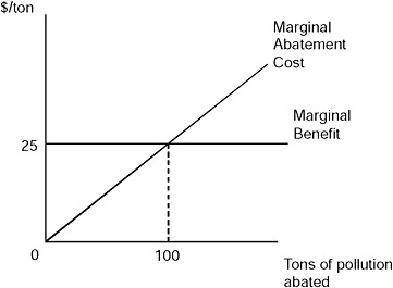
FIGURE B-1 Pollution abatement (horizontal axis) and cost per ton of abatement (vertical axis).
for this plant is $25 per ton. In practice, the shape of this curve will be pollutant-specific (and might well be location- and time-specific).
Society is made better off if the firm increases its abatement from 0 to 100 tons. The benefit to society is the avoided damages of $25 per ton times the 100 tons abated, or $2,500. The cost to the firm of reducing its pollution is the sum of the incremental abatement costs. This is the area under the marginal abatement curve and it equals $1,250. The net gain to society following the firm’s abatement action is $1,250.
Is 100 tons of pollution abatement the economically optimal amount? All other things being equal, the answer is yes. More generally, the economically optimal level of pollution abatement occurs at the point where marginal benefits equal marginal costs. To see why, consider an additional ton of abatement from 100 to 101 tons. The benefit to society is $25. The marginal cost, however, is an amount greater than $25 because the marginal abatement curve rises above $25 for abatement levels greater than 100. For abatement levels greater than 100 tons, the incremental abatement costs to the firm outweigh the incremental benefits to nearby residents. Similarly, any level of abatement below 100 tons are not economically optimal. At any level less than 100 tons, the cost to the firm of reducing pollution by 1 more ton is less than the benefit to nearby residents of that incremental pollution reduction.
Note, however, that the illustrative example does not include consider-
ation of important distributional issues by simply summing the costs and benefits of pollution reduction. Distributional considerations can be taken into account. They will affect the economically optimal level of pollution abatement in the example but not the fundamental concepts that the example illustrates.


