
Autonomy Under Water: Ocean Sampling by Autonomous Underwater Vehicles
DEREK A. PALEY
University of Maryland
The ocean is large and opaque to electromagnetic waves used for communication and navigation, making autonomy under water essential because of intermittent, low-bandwidth data transmission and inaccurate underwater positioning. Moreover, the vastness of the ocean coastlines and basins renders traditional sampling time-consuming and expensive; one typically must make do with sparse observations, which leads to the question of where to take those measurements. Further complicating the problem, circulating ocean processes pertinent to national defense and climate change span small to large space and time scales, necessitating multiple sampling platforms or vehicles, ideally with long endurance.
Many effective vehicle designs are not propeller-driven but rather buoyancy-driven; becoming heavy or light relative to the surrounding seawater generates vertical motion suitable for collecting profiles of hydrographic properties such as salinity, density, and temperature. Buoyancy-driven vehicles drift with the currents unless they have wings, in which case their vertical motion is converted to horizontal motion via lift, like an air glider. The capacity to maneuver relative to the flow field gives rise to challenges in cooperative control and adaptive sampling with the following recursive property: vehicles collect measurements of the ocean currents in order to estimate it; the estimate is used to guide the collection of subsequent measurements along sampling trajectories subject to currents that may be as large as the platform’s through-water speed.
Approaches to adaptive sampling of continuous environmental processes are distinguished by the characterization of the estimated process as statistical or dynamical. A statistical characterization involves spatial and temporal decorrelation scales, which for a nonstationary process may vary in space and time.
Presuming these scales are known, the challenge is to distribute measurements proportionally to the local variability—highly variable regions require higher measurement density—to minimize the so-called mapping error. If the scales are unknown, the challenge is twofold: they must be estimated while concurrently using estimated scales for mapping.
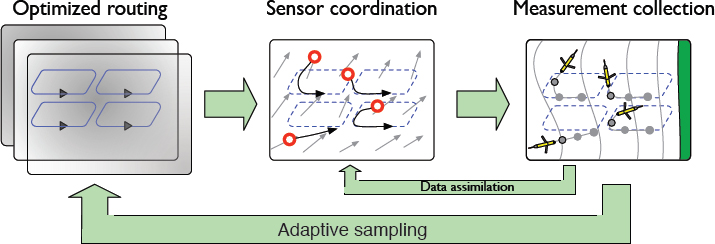
A dynamical characterization of the estimated process replaces the decorrelation statistics with the differential equations that govern the evolution in time of the process parameters. Dynamical descriptions permit the application of tools from systems theory, including the concept of observability, which measures the sensitivity of a system’s outputs to perturbations of the system’s states about a nominal value. The selection of where to collect sensor observations (i.e., where to route the sensor platforms) is thus formulated as the problem of maximizing the observability of a nonlinear dynamical system. Because observability is traditionally a forward-looking metric, it is augmented with estimation uncertainty in order to account for locations of prior observations. Figure 1 depicts the adaptive-sampling feedback loop.
DISTRIBUTED ESTIMATION OF SPATIOTEMPORAL FIELDS
Observability-based optimization in path planning (Yu et al. 2011) and data assimilation (Krener and Ide 2009) typically uses either a low-dimensional parameterized model or an empirical data-based representation of the unknown process; however, problems arise when neither a suitable model nor sufficient data are available. The novelty of the approach described here lies in the use of the observability of a low-dimensional model of an environmental vector field and a data assimilation filter to guide the observability analysis via metrics from Bayesian experimental design. Observability- and information-based optimization
of sampling trajectories yields a reliable and predictable capability for intelligent, mobile sensors. A dynamic, data-driven Bayesian nonlinear filter exploits noisy, low-fidelity, and nonlinear measurements collected in a distributed manner by combining observations from individual or multiple sampling platforms.
Although methods exist for the optimization of sampling trajectories using distributed parameter estimation (Demetriou 2010), optimal interpolation (Leonard et al. 2007), and heuristic approaches (Smith et al. 2010), an open question is how to rigorously characterize the variability of information content in an unknown spatiotemporal process and how to target observations in information-rich regions. The merit of the approach described here lies in the design of a statistical framework based on spatiotemporal estimation of nonstationary processes in meteorology (Karspeck et al. 2012) and geostatistics (Higdon et al. 1999). The framework extends my previous work in this area into multiple dimensions and builds a nonstationary statistical representation of a random process while simultaneously optimizing the sampling trajectories.
In oceanography, autonomous underwater vehicles are used as mobile sensors for adaptive sampling. Indeed, the concept of optimal experimental design was first applied to oceanographic sampling in the 1980s (Barth and Wunsch 1990). The optimization of sensor placement and data collection has applications in fighting wildfires, finding perturbation sources in power networks, and collecting spatial data for geostatistics. Perhaps it is not surprising, given the range of these applications, that there are a variety of approaches advocated in the literature, including adaptation based on maximum a posteriori estimation, stochastic deployment policies, information-based methods, learning and artificial intelligence, deterministic methods with heuristic metrics, bioinspired source localization and gradient climbing, and nonparametric Bayesian models.
The results described here differ from prior work on adaptive sampling of dynamical systems and random processes in the novel application of nonlinear observability and control coupled with recursive Bayesian filtering to optimize sensor routing for environmental sampling. One approach to adaptive sampling in the ocean uses observability: a measure of how well the state variables of a control system can be determined by measurements of its outputs.
Observability of a linear system (Hespanha 2009) is characterized using the Kalman rank condition, which is a special case of the observability rank condition of a general, nonlinear system (Hermann and Krener 1977). (A nonlinear system is called observable if two states are indistinguishable only when the states are identical.) Observability in data assimilation refers to the ability to determine the parameters of an unknown process from a history of observations.
Although standard observability tests give a binary answer (i.e., the system is observable or not), the degree of observability may be computed from the singular values of the observability gramian (Krener and Ide 2009), a Hermitian matrix containing inner products of the system’s outputs under systematic perturbations of the system’s parameters about a nominal value. Computation of the empiri-
cal observability gramian requires only the ability to simulate the system and is therefore particularly attractive for numerical optimization.
A second approach to adaptive sampling is based on classical estimation theory (Liebelt 1967): optimal statistical interpolation of sensor observations to produce a stochastic estimate of an unknown random process, formerly known in meteorology and oceanography as objective analysis (Bretherton et al. 1976). Optimal interpolation also yields a measure of the uncertainty or error in the estimate, which can be used as a measure of estimator performance or skill (Leonard et al. 2007). It is common to compute estimation error under the assumption of stationarity of the spatial and temporal variability of the unknown process, although these assumptions may not be borne out in applications of interest. A stochastic process whose variability changes when shifted in time or space is called nonstationary, and methods exist to parameterize nonstationary processes in oceanography and geostatistics. Indeed, nonstationary-based strategies have been applied to mobile sensor networks, though not based on a principled control design.
DATA-DRIVEN ADAPTIVE SAMPLING: MEASURES OF OBSERVABILITY
The observability of a nonlinear system may be difficult to determine analytically, because it requires tools from differential geometry (Hermann and Krener 1977). If the dynamical model of interest is solved numerically, numerical techniques can be used to calculate the empirical observability gramian (Krener and Ide 2009). This gramian does not require linearization, which may fail to adequately model the input-output relationship of the nonlinear system over a wide range of operating conditions, but merely the ability to simulate the system. Indeed, it maps the input-output behavior of a nonlinear system more accurately than the observability gramian produced by linearization of the nonlinear system.
The empirical observability gramian is a square matrix whose dimension matches the size of the state vector and whose (i,j)th entry represents the sensitivity of the output to infinitesimal perturbations about their nominal value of the corresponding i and j states or unknown parameters. The observability of a nonlinear system is measured by calculating the unobservability index ν of the empirical observability gramian. This index is used to score candidate trajectories for their anticipated information gain. Figure 2 depicts an observability-based feedback loop, including a recursive Bayesian filter to assimilate noisy measurements from the observing platforms.
DATA-DRIVEN ADAPTIVE SAMPLING: MAPPING ERROR
A spatiotemporal field is statistically described by its mean and the covariance function between any two points i and j. A covariance function is a positive-
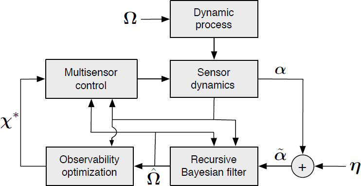
 corrupted by noise η. The estimated parameters are used to calculate observability-optimizing control parameters χ* that characterize the multisensor sampling formation.
definite function that describes the variability of the field between the ith and jth locations (Bennett 2005). A field is stationary if its covariance function depends only on the relative position of i and j, and it is nonstationary if it depends on i and j independently.
There are a number of choices for the form of a nonstationary covariance function, e.g., Matern, rational quadratic, Ornstein-Uhlenbeck, and squared-exponential forms (see Higdon et al. 1999). A statistics-based sampling strategy requires a covariance function that is a product of spatial- and temporal-covariance functions, such as a nonstationary squared exponential covariance function. In this case, the square roots of the diagonal elements are the spatial and temporal decorrelation scales of the field. (The decorrelation scales are the spatial and temporal separations at which the covariance function evaluates to 1/e.) For a stationary field the decorrelation scales are constant, whereas for a nonstationary field they may vary in space and time. The covariance function is used to derive a coordinate transformation that clusters measurements in space-time regions with short decorrelation scales and spreads measurements elsewhere, where the measurement demand is lower.
Statistics-based sensor routing seeks to provide optimal coverage of an estimated spatiotemporal field. The coverage is deemed optimal when the measurement density in space and time is proportional to the variability of the field. To determine when measurements are redundant, consider the footprint of a measurement, defined as the volume in space and time in an ellipsoid centered at the
measurement location with principal axes equal to the decorrelation scales of the field. The goal is to design the vehicle trajectories so that the swaths created by the set of all measurement footprints cover the entire field with minimal overlaps or gaps, even when the decorrelation scales of the field vary.
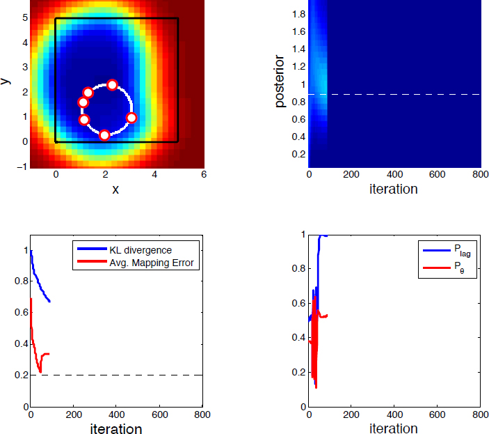
Optimal interpolation is used to determine the mapping error (Bennett 2005), which is the diagonal of the error covariance matrix. The average (resp. maximum) mapping error is computed by averaging (resp. finding the maximum of) all the elements of the mapping error. Because the vehicles sample uniformly in time, the mapping error is minimized in a stationary field by traveling at maximum speed to place as many measurements as possible in the domain (Sydney and Paley 2014). Figure 3 depicts the mapping error for a stationary field with a correlation scale estimated by a Bayesian filter.
REFERENCES
Barth N, Wunsch C. 1990. Oceanographic experiment design by simulated annealing. Journal of Physical Oceanography 20(9):1249–1263.
Bennett AF. 2005. Inverse Modeling of the Ocean and Atmosphere. Cambridge, UK: Cambridge University Press.
Bretherton FP, Davis RE, Fandry CB. 1976. A technique for objective analysis and design of oceanographic experiments applied to MODE-73. Deep-Sea Research 23(7):559–582.
Demetriou MA. 2010. Guidance of mobile actuator-plus-sensor networks for improved control and estimation of distributed parameter systems. IEEE Transactions on Automatic Control 55(7):1570–1584.
Hermann R, Krener AJ. 1977. Nonlinear controllability and observability. IEEE Transactions on Automatic Control 22(5):728–740.
Hespanha J. 2009. Linear Systems Theory. Princeton, NJ: Princeton University Press.
Higdon D, Swall J, Kern J. 1999. Non-stationary spatial modeling. Bayesian Statistics 6(1):761–768.
Karspeck AR, Kaplan A, Sain SR. 2012. Bayesian modelling and ensemble reconstruction of mid-scale spatial variability in North Atlantic sea-surface temperatures for 1850–2008. Quarterly Journal of the Royal Meteorological Society 138(662):234–248.
Krener AJ, Ide K. 2009. Measures of unobservability. Proceedings of the IEEE Conference on Decision and Control, pp. 6401–6406, Shanghai, December 16–18.
Leonard NE, Paley DA, Lekien F, Sepulchre R, Fratantoni DM, Davis RE. 2007. Collective motion, sensor networks and ocean sampling. Proceedings of the IEEE 95(1):48–74.
Liebelt PB. 1967. An Introduction to Optimal Estimation. Reading, MA: Addison-Wesley.
Smith SL, Schwager M, Rus D. 2010. Persistent robotic tasks: Monitoring and sweeping in changing environments. IEEE Transactions on Robotics 28(2):410–426.
Sydney N, Paley DA. 2014. Multivehicle coverage control for nonstationary spatiotemporal fields. Automatica 50(5):1381–1390.
Yu H, Sharma R, Beard RW, Taylor CN. 2011. Observability-based local path planning and collision avoidance for micro air vehicles using bearing-only measurements. Proceedings of the American Control Conference, pp. 4649–4654, June 29–July 1, San Francisco.
This page intentionally left blank.


