
4
The Impact of Southern Ocean Circulation and Air–Sea Exchange on Global Heat and Carbon Budgets
Climate change due to increased atmospheric carbon dioxide (CO2) will have significant impacts on the national and global economy. Warmer temperatures can cause economic loss in many ways, including lowering agricultural yields, decreasing industrial output, and damaging infrastructure (USGCRP, 2018). Over the past decade, direct damages related to climate change have been estimated at approximately $1.3 trillion (Suntheim and Vandenbussche, 2020). A warming climate can also lead to adverse health effects, such as increased respiratory and cardiovascular disease, premature death due to extreme weather events, and changes in the prevalence and geographical distribution of infectious diseases (CDC, 2020). Current and future policy decisions related to climate resilience and adaptation will rely heavily on predictions from coupled climate models. Validation of these models remains an ongoing priority for the climate community, with validation of the role of the Southern Ocean and Antarctic coastal regions in the global climate system being particularly challenging because of sparse observations.
The Southern Ocean’s key role in global ocean circulation and Earth’s climate is largely due to the unimpeded flow of its waters from west to east—connecting the Atlantic, Pacific, and Indian basins—that impact water properties globally (Gordon, 1986; Talley, 2013). The absence of north–south continental boundaries between Antarctica and continents to the north has dynamical consequences that greatly affect the global climate (Olbers et al., 2004). First, the Earth’s only circumpolar current, the Antarctic Circumpolar Current (ACC), resides in the Southern Ocean (Figure 4-1). The ACC is characterized by vigorous ocean eddies and jets that both connect different ocean regions and mix water properties. This mixing establishes global heat, nutrient, and dissolved gas concentrations with implications for ocean energetics (Wunsch and Ferrari, 2004), ocean heat uptake (Armour et al., 2016), atmospheric greenhouse gas concentrations (Gruber et al., 2019a,b), and marine primary productivity (Moore et al., 2018). Second, throughout most of the ocean, different water masses are layered horizontally, with lighter waters at shallower depths and denser waters at deeper depths. Globally, these deep waters hold roughly 60 times the amount of carbon in the atmosphere and have taken up almost 95 percent of excess heat in recent decades (DeVries, 2014; Gruber et al., 2019a,b). This layered structure limits the exchange of deep carbon-rich waters with near-surface waters and the atmosphere. In the Southern Ocean, however, this layering of lighter and denser waters acquires a tilt away from horizontal, associated with the flow of the ACC, such that deep water masses reach the surface without having to mix with lighter-density layers (Marshall and Speer, 2012). Thus, dense waters can access the ocean surface only in the Southern Ocean, giving this region an outsized impact on global water properties. In fact, surface waters south of 35°S represent only 20 percent of the world’s surface ocean but account for 40–50 percent of the total removal of fossil fuel
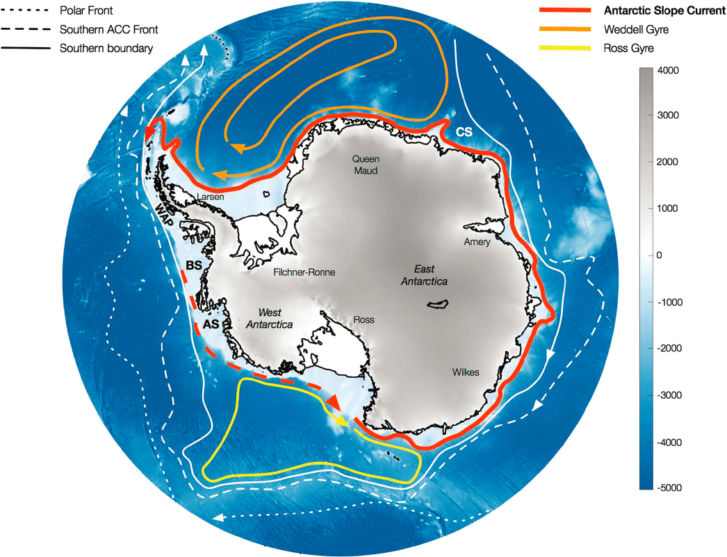
NOTES: The Antarctic Circumpolar Current (ACC) is composed of various fronts that separate different water properties. These properties are roughly homogeneous in the along-stream (east–west) direction but change abruptly in the north–south direction. The subpolar gyres tend to mix and homogenize physical and biogeochemical properties, but the Antarctic Slope Front, associated with the Antarctic Slope Current, supports abrupt transitions between offshore and continental shelf water properties. Dashed red line on Antarctic Slope Current indicates uncertain initiation. AS = Amundsen Sea; BS = Bellingshausen Sea; CS = Cosmonauts Sea; WAP = Western Antarctic Peninsula.
SOURCE: Figure adapted from Thompson et al., 2018.
CO2 emissions (DeVries, 2014; Gruber et al., 2019a,b). However, the exact flux of CO2 between the Southern Ocean atmosphere and ocean is not well constrained as atmospheric inversion (Long et al., 2021), and surface floats measurements (Gray et al., 2018) provide slightly different estimates (see discussion below). The Southern Ocean’s unique density structure also has implications for how waters fill the deep ocean (Purkey et al., 2018), how nutrients are delivered to low latitudes (Sigman et al., 2010), how heat is delivered to the Antarctic ice shelves (Tamsitt et al., 2017), and how older water masses exchange dissolved gases with the atmosphere when brought back to the surface (Morrison et al., 2022; Sarmiento and Toggweiler, 1984).
The ACC is the dominant and most energetic circulation feature of the Southern Ocean, but it is only one part of an intricate circulation system that connects the Atlantic, Pacific, and Indian basins to the Antarctic coastline. Properties that exit the ACC to the south are fed into subpolar gyres, which are clockwise-circulating features that
bridge the ACC and the Antarctic continental slope and shelf (Sonnewald et al., 2023; Vernet et al., 2019). The subpolar gyres influence the formation, redistribution, and melt of sea ice and icebergs in the Southern Ocean; they also influence ocean carbon uptake through organic matter production in the center of the gyre and redistribution by the gyre’s horizontal circulation (MacGilchrist et al., 2019). There remains limited understanding of how these large circulation features will respond to a combination of modified atmospheric forcing, changing sea ice extent, and increased freshwater input from ice shelf and glacial ice losses, all of which have been observed and all of which are expected in a warming climate.
Along the southern boundary of the subpolar gyres above the Antarctic continental slope, relatively warm waters—a few degrees above freezing—rise up toward the continental shelf. In this location, a combination of shallower bathymetry, surface wind forcing, and water properties of the continental shelf contribute to the formation of the Antarctic Slope Front (ASF). The ASF acts as a key dynamical gateway for the delivery of heat to ice shelf cavities and the grounding zones of the Antarctic ice sheets (Chapter 3; Thompson et al., 2018). The properties of the ASF and its contribution to on-shelf heat transport vary around Antarctica. Some shelf seas are flooded by warm waters, such as the western Antarctic Peninsula and the Amundsen Sea, while others are cold and fresh, such as much of East Antarctica (Schmidtko et al., 2014; Stewart et al., 2018). Despite predominantly cold and fresh waters over the East Antarctic continental shelf, localized intrusions of warm waters have been documented regionally, particularly in waters near the Totten (Rintoul et al., 2016) and Amery (Guo et al., 2022) ice shelves. While direct measurements of ocean water in ice shelf cavities and ocean–ice interactions are essential (Chapter 3), monitoring the evolution of continental shelf properties may provide early indication of changes in ice shelf melting patterns and potential Antarctic ice sheet destabilization. Additionally, injection of ice shelf meltwater has a strong impact on the local stratification and circulation of the seas surrounding the ice shelf (Silvano et al., 2018), as well as the formation of dense shelf waters1 (Jacobs et al., 2022; Li et al., 2023) and ice shelf melt (Flexas et al., 2022) in remote regions.
Along the Antarctic coast, physical processes that involve coupling between the ocean, sea ice, Antarctic ice shelves, and the atmosphere produce water properties associated with Antarctic Bottom Water (AABW), which is the coldest and densest type of water found in the global ocean (Figure 4-2; Orsi et al., 1999). AABW is formed in polynyas, which are regions of open ocean surrounded by sea ice that form because of persistent katabatic winds.2 These polynyas are sites of extreme heat loss, intense CO2 exchange with the atmosphere, and dense shelf water formation—particularly in the Weddell and Ross seas. Their sustained heat loss to the atmosphere and associated sea ice formation lead to the formation of cold, dense water that flows down the continental slope and spreads along the ocean bottom as AABW, covering close to 80 percent of the global seafloor (Purkey et al., 2018).
As AABW fills the deep ocean, it determines abyssal ocean stratification, or the change in density with depth that regulates the timescale over which heat and carbon can be sequestered in the deep ocean. Today, carbon taken up by the ocean near the Antarctic coast can be carried to depth as AABW and sequestered for many hundreds to a thousand years. In recent decades, less AABW has been produced, and that which is produced has warmed and freshened, which impacts the global overturning circulation (Figure S-2; Purkey and Johnson, 2010, 2012, 2013). The dynamical processes responsible for setting the volume and properties of AABW are both poorly understood and have traditionally been poorly represented in global climate models (Heuzé et al., 2013). However, newer models with higher resolution have shown that increases in oceanic freshwater content have the potential to reduce the production of AABW and lead to a substantial slowdown of the lower cell of global overturning circulation (Gunn et al., 2023; Li et al., 2023).
Paleoclimate data demonstrate that the Southern Ocean has a strong control on glacial–interglacial cycles in atmospheric CO2 concentrations and global ocean heat content. These changes have been linked to fluctuations in the efficiency with which deep-ocean carbon and heat are taken up or released to the atmosphere. These fluctuations are caused by a reorganization of the density classes that fill the abyssal ocean and outcrop at the ocean surface, enhanced Southern Ocean ice coverage that acts as a barrier to surface CO2 exchange, and changes in
___________________
1Dense shelf water is cold and salty water that is the precursor to Antarctic Bottom Water.
2Katabatic winds are often produced from cold, dense air over ice sheets that “blow[s] down a slope because of gravity” (Britannica Editors, 2020, para. 1).
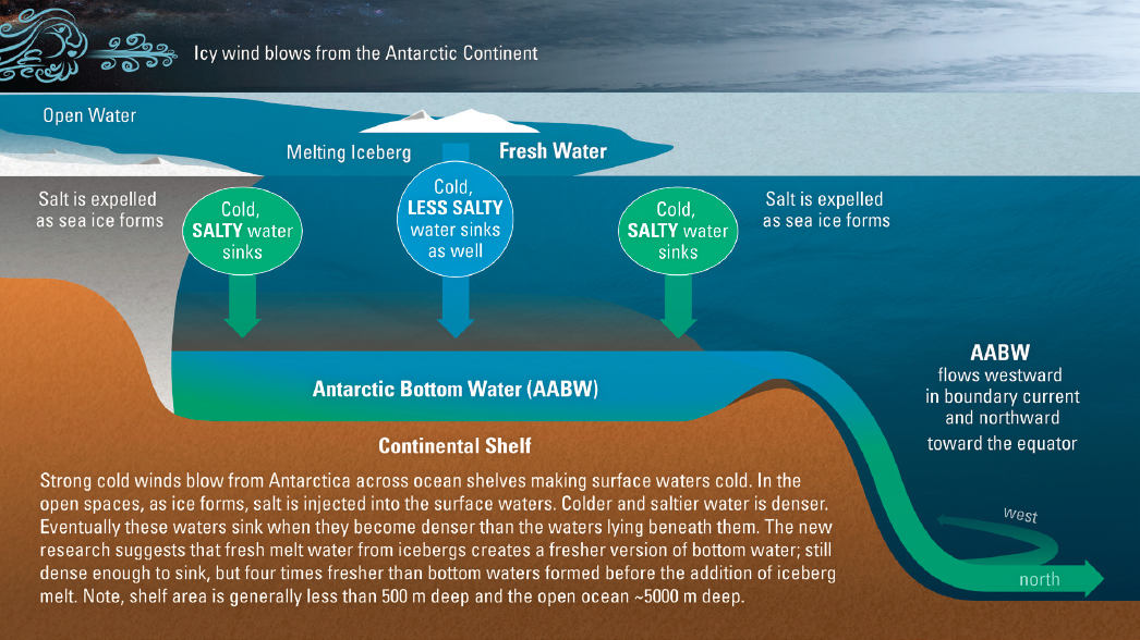
SOURCE: WHOI, 2017. ©Woods Hole Oceanographic Institution.
upper-ocean stratification that reduce vertical mixing (Ferrari et al., 2014; Keeling and Stephens, 2001). Current estimates of air–sea carbon fluxes are often relatively small, which might seem contradictory to the assertion that Southern Ocean waters are a net sink for CO2. However, these estimates need to be placed in the context of the preanthropogenic system in which the Southern Ocean experienced upwelling deep waters, making it a large source of natural CO2 emissions. As atmospheric pCO2 (partial pressure of CO2) has increased, the air–sea pCO2 difference and resulting oceanic CO2 emissions decrease. When this water sinks into the interior, it carries more CO2 than before the anthropogenic perturbation. Hence, it becomes a net sink in the global ocean CO2 system; for this reason, repeat CO2 surveys show that CO2 in Southern Ocean waters is increasing (Gruber et al., 2019a,b).
Present-day variations in the magnitude of the region’s air–sea carbon flux remain poorly constrained. Uncertainty in the magnitude of these fluxes is greater in more southern regions, and the magnitude is especially poorly constrained south of 60°S. Additionally, modeling estimates of integrated air–sea CO2 fluxes disagree substantially on decadal-scale variability of the Southern Ocean carbon sink. Observational estimates suggest a substantial weakening of carbon uptake in the 1990s that models do not reproduce (Gruber et al., 2019a,b; Landschützer et al., 2015; Le Quéré et al., 2007). It remains unclear whether ocean models are missing key dynamics, such as ocean eddies in coupled models, or whether there are errors inherent in extrapolating a sparse dataset, especially in winter months, to the circumpolar Southern Ocean (Gruber et al., 2019a,b). This disagreement impacts confidence in the analysis of long-term trends and makes it difficult to arrive at a mechanistic attribution of carbon-flux changes (McKinley et al., 2017).
This chapter outlines the highest-priority scientific questions that will allow the scientific community to determine the impact of Southern Ocean circulation and air–sea exchange on global heat and carbon budgets. Each section also expands on the observations and capabilities that are necessary to advance the state of knowledge. Five priority science questions are identified: (1) What determines the net uptake and release of CO2 in the
Southern Ocean and how will it change in the future? (2) What are the key temporal and spatial scales of upper-ocean processes that influence air–sea exchange? (3) What are the pathways of ocean heat and biogeochemical properties between the open Southern Ocean and the Antarctic coast? (4) How can understanding past changes in the Southern Ocean heat and CO2 budgets elucidate the future? (5) What processes will impact Antarctic sea ice extent and thickness on decadal timescales?
WHAT DETERMINES THE NET UPTAKE AND RELEASE OF CO2 IN THE SOUTHERN OCEAN AND HOW WILL IT CHANGE IN THE FUTURE?
Water sinking to intermediate and greater depths in the Southern Ocean with above-preanthropogenic levels of dissolved CO2 is responsible for about 40–50 percent of the net removal of fossil fuel CO2 emissions (Watson et al., 2014). Spatially and temporally extensive measurements of the dissolved inorganic CO2 inventory in the water column and the partial pressure difference between the sea surface and atmosphere are required in order to create an accurate inventory of accumulated excess inorganic carbon and to model and predict future levels of CO2 in the atmosphere. Precise measurements of related nutrient and biological levels, like iron content, also allow for the evaluation of the biological carbon pump’s role in lowering atmospheric CO2 (Chapter 5).
Currently, precise CO2 inventories and related nutrient and biological measurements can only be obtained by shipboard water sampling. Although there are literally millions of pCO2 change measurements performed by automated systems on research vessels and merchant ships, such measurements are extremely limited in the Southern Ocean, especially in the crucial winter periods, when water mass formation and sinking is active. Non-icebreaking vessels can obtain these data from north of 60°S and slightly further south when waters are predictably ice free. When performed closer to the Antarctic continent, obtaining these measurements requires icebreakers that can travel through significant amounts of sea ice. Without investment in a new icebreaker with appropriate sampling gear, the United States will be unable to precisely monitor ocean CO2 and related physical, biogeochemical, and biological properties in the Southern Ocean. Should a new icebreaker have better icebreaking capabilities than currently available, the United States would be able to extend its CO2 monitoring much closer to the Antarctic coast.
Temporally and spatially extensive monitoring of the air–sea CO2 difference has recently been enabled by drifter, glider, floats, autonomous underwater vehicle (AUV), and autonomous surface vehicle technology. These technologies measure the pCO2 difference, or calculate it from pH, and determine the resulting CO2 flux using concurrent wind speed and gas exchange-rate formulations. A caveat is that the CO2 flux requires an estimate of alkalinity, which at present is derived from a climatological relationship with mobile sensor data on temperature, salinity, oxygen, and nitrate. Locally, the alkalinity may deviate from this relationship substantially, contributing to uncertainty in the CO2 flux (Carter et al., 2018). One important technology utilized for these measurements is biogeochemical Argo (BGC-Argo) floats, which drift passively and periodically (usually once every 10 days) acquire a vertical profile of physical and biogeochemical properties in the upper 2000 m of the ocean. The Southern Ocean Carbon and Climate Observations and Modeling (SOCCOM) project has seeded the Southern Ocean with 265 BGC-Argo floats (as of April 2023), vastly improving circumpolar maps of biogeochemical tracer distributions, especially in winter months. Even though SOCCOM’s success is based on multiseasonal pCO2 measurements, understanding the processes requires shipboard alkalinity, oxygen, and nitrate measurements to improve the climatological alkalinity estimate, requiring continued icebreaking capability for Antarctic water column sampling.
An initial analysis from a small number of the SOCCOM floats found stronger CO2 outgassing in the Southern Ocean’s polar and seasonal ice zone regions as compared to earlier estimates (Gray et al., 2018). This discrepancy remains unexplained, with a recent study finding strong carbon uptake south of 45°S (Long et al., 2021). These studies use different methods, with the former using sea surface pCO2 and the latter using airborne observations of atmospheric CO2 gradients. The relative reliability of these approaches remains uncertain, especially as air–sea fluxes are likely spatially heterogeneous and temporally intermittent (Brady et al., 2021; Nicholson et al., 2022), depending on both geographical and dynamical properties (Dove et al., 2022; Langlais et al., 2017). The character and variation of these small-scale fluxes are not yet captured in Coupled Model Intercomparison Project–class climate models.
While there has been recent success with operating Argo platforms in shallow waters (Wallace et al., 2020), BGC-Argo floats have limited capabilities under sea ice and are not designed to sample in waters shallower than 2000 m, which excludes the Antarctic continental shelf. Thus, carbon fluxes within the Antarctic sea ice zone, including in polynyas, remain even more weakly constrained than in the ACC. Sparse observations of how oceanic carbon content varies with seasonal surface fluxes and large phytoplankton blooms lends large uncertainty to how these localized regions contribute to the global carbon cycle. Lack of year-round observations may also bias the estimation of annual CO2 flux in Antarctic polynyas to levels observed in summer because few observations exist in the fall, winter, and spring (Arrigo et al., 2008). Emerging developments in pCO2 sensors that can be deployed on ice-capable floats and gliders can expand observations to cover the entire Southern Ocean and may improve the accuracy of autonomous observations in the future. Challenges remain in measuring gas fluxes in ice-covered waters, where sea ice can act both as an exchange barrier and a source of CO2 (Delille et al., 2014). While the sea ice cover limits gas exchange between the ocean and atmosphere, modeling suggests that in the spring and summer period, sea ice may be responsible for more than half of the CO2 uptake in the seasonal ice zone due to a combination of dissolution of ice brine and solid salts, as well as sea ice primary productivity, but the contributions of these processes are highly uncertain (Delille et al., 2014). At present, autonomous observations of these processes are not practical, so understanding the role of sea ice and sea ice biology in the seasonal cycle of CO2 exchange will continue to require vessel access into the ice. As sensor and platform technology evolves, new CO2 sensors and floats and under-ice gliders will enable greater spatiotemporal coverage throughout the Southern Ocean.
WHAT ARE THE KEY TEMPORAL AND SPATIAL SCALES OF UPPER-OCEAN PROCESSES THAT INFLUENCE AIR–SEA EXCHANGE?
The exchange of heat and climatically relevant trace gases across the air–sea interface in the Southern Ocean has an oversized impact on global climate because a large fraction of the global ocean’s deepest waters access the surface in this region. Processes that set rates of heat and carbon uptake at the air–sea interface may span a range of temporal and spatial scales, but ultimately involve small-scale turbulent properties of atmospheric and oceanic boundary layers (Bourassa et al., 2013; Swart et al., 2020). Direct measurements of these surface fluxes are sparse, especially in regions south of the Polar Front, including the seasonal sea ice zone and near-coastal regions. Such observations of heat, gas, and mass (i.e., precipitation and evaporation) are of particular importance in the Southern Ocean, where errors in flux budgets can be very large (Bourassa et al., 2013). Few field programs have acquired direct observations of surface fluxes that couple the atmosphere, ocean, and ice in the Southern Ocean; therefore, there are limited constraints on the variability of these fluxes that could be compared with their representation in coupled climate models (Swart et al., 2023).
There is a growing awareness that ocean dynamics occurring at the mesoscale (50–100 km) and the submesoscale (1–50 km) contribute to setting circumpolar properties of air–sea exchange (Seo et al., 2023). Similarly, temporally intermittent processes (e.g., storms, fluctuation of sea ice extent) can set circum-Antarctic annual rates of CO2 exchange (Nicholson et al., 2022; Patoux et al., 2009). Thus, there is a need to link the broad, low-frequency sampling carried out by BGC-Argo floats with growing evidence that carbon exchange across the air–sea interface and into the ocean interior is spatially localized and intermittent (Brady et al., 2021). Physical processes at these scales are dominated by coherent structures such as eddies, fronts, meanders, and filaments, many of which support enhanced vertical velocities that connect the ocean’s surface boundary layer to the interior (Morrison et al., 2022) and shape the marine carbon cycle up to the climate scale (Lévy et al., 2018). These features are not well sampled spatially by BGC-Argo-style floats, and they also typically evolve too quickly for sampling with existing AUVs. Autonomous surface platforms, such as Wave Gliders and Saildrones, are better suited to obtain these measurements, as they have the potential to provide long-duration observations on rapidly moving platforms (assuming there is sufficient light for solar power). In addition, the development of low-cost, expendable Lagrangian floats3 would allow for the simultaneous deployment of many tens to hundreds of drifting platforms to capture relevant dynamics. Regardless, ship-based field work with capabilities for chemical and biological sampling and rapid
___________________
3Lagrangian floats do not move on their own, but instead drift passively in the ocean (Schmidt Ocean Institute, 2023).
underway sampling4 will remain the primary mechanism for building process-based studies of air–sea fluxes in at least the coming decades. Further, there is a need to couple this process-based understanding with efforts to develop satellite-based measurements of surface fluxes, such as those currently being considered for surface heat and momentum fluxes.
Mesoscale and submesoscale coupling between the ocean and atmosphere are not captured in global climate models, and it is unclear how much fine-scale processes impact climate projections (Hewitt et al., 2022). The Southern Ocean is particularly important in this respect because of its disproportionate role in contributing to climate variability (Gregor et al., 2018; Marinov et al., 2006) and because it is associated with high mesoscale activity. Addressing how fine-scale processes impact longer-term climate change requires innovative experimental designs, likely involving heterogeneous arrays of autonomous vehicles coupled with multiple satellite missions (e.g., sea surface height from both radar and laser altimeters, surface temperature, ocean color), along with high-resolution coupled models (Fox-Kemper et al., 2019) that can adequately interrogate the physical–biological and ocean–atmosphere coupling of processes in the Southern Ocean.
WHAT ARE THE PATHWAYS OF OCEAN HEAT AND BIOGEOCHEMICAL PROPERTIES BETWEEN THE OPEN SOUTHERN OCEAN AND THE ANTARCTIC COAST?
Ocean circulation over the continental slope and shelf delivers heat to floating Antarctic ice shelves and sea ice, supplies nutrients to regions of high primary productivity in polynyas, and contributes to setting properties of AABW. The production and characteristics of AABW, in turn, influence the strength of the lower limb of the global overturning circulation and carbon sequestration (Li et al., 2023; Purkey et al., 2018). Modification to water properties, which support the continental shelf overturning circulation, occur near the coast in ice shelf cavities and coastal polynyas. It is near the coast where cyclonic circulations5 that connect the shelf break and the coast via bathymetric troughs interact with the surface-trapped Antarctic Coastal Current,6 convective mixing in polynyas linked to sea ice production, boundary current inflows and outflows of ice shelf cavities, and gyres steered by topographic depressions. Interactions between these components of shelf circulation set the vertical and lateral stratification of the water column, influencing geostrophic flow,7 as well as the transport of heat, CO2, and nutrients at the ice shelf face. Few observational campaigns have captured the spatial and temporal scales of variability of these dynamic features, and no field program has achieved sustained measurements of this region during winter conditions. Observing a full seasonal cycle is needed to discern long-term trends from natural variability governed by surface wind and buoyancy forcing. Because of significant interannual variability across the continental shelf, these year-round observations need to be sustained over multiple years.
The limited ability to constrain how oceanic forcing of Antarctic ice shelves by Circumpolar Deep Water (CDW) will change in a warming climate is a key driver of uncertainty in future projections of the Antarctic ice sheets’ contribution to sea level rise (Chapter 3; Edwards et al., 2021; Seroussi et al., 2014), as well as in future projected changes to the AABW and its influence on carbon uptake in the Southern Ocean (Li et al., 2023; Purkey et al., 2018). Previous studies have explored temporal changes in the temperature of CDW (Schmidtko et al., 2014), as well as interannual variations in the thickness or heat content of the CDW layer (Dutrieux et al., 2014a; Jenkins et al., 2018). While CDW has warmed slightly, roughly 0.1°C to 0.2°C per decade in West Antarctic shelf seas, CDW thickness can vary by many hundreds of meters on interannual or potentially shorter timescales. This variation in thickness has been identified as the key driver of basal melt variability in the Amundsen Sea (Jenkins et al., 2018).
Drivers of temporal variations in CDW have largely focused on forcing at the shelf break, with surface wind forcing identified as the main mechanism for modulating the shoreward transport of CDW across the shelf break
___________________
4Underway measurements can include continuously sampled hull-based water intake to packages or instrument platforms that are towed behind the ship.
5Cyclonic circulation is movement in the same direction as the Earth’s rotation.
6 The Antarctic Coastal Current is a buoyant, fresh current that flows westward along the coast and face of Antarctic ice shelves.
7Geostrophic flow refers to velocities that arise from a balance between pressure gradients and the Coriolis force in a rotating system; geostrophic velocities are oriented perpendicular to the direction of the pressure gradient. Most flows in the ocean at scales larger than about 10 km are in geostrophic balance.
(Thoma et al., 2008). Both observational and modeling studies have presented compelling correlations between the shoreward transport of CDW through the Dotson-Getz and Pine Island–Thwaites troughs and wind forcing over the continental shelf (Dotto et al., 2019; Kim et al., 2017, 2021; Silvano et al., 2022; Webber et al., 2019), although research into the dynamics underlying this relationship is ongoing. These studies have established a paradigm in which wind-driven variability of CDW transport onto the continental shelf modifies the thickness of the CDW layer and thus the observed decadal-scale change in the Amundsen Sea embayment’s heat content. This perspective, however, focuses on the supply of CDW, which does not account for physical processes over the continental shelf that modify or erode this warm water layer. For instance, wind-driven mechanisms have yet to explain why the amplitude of observed CDW thickness changes and simulated variability increases substantially toward the coast (Kim et al., 2021; Silvano et al., 2022). Years with a thick CDW layer (2006–2011) are consistently associated with stronger stratification and larger contributions from glacial meltwater in the upper ocean, as compared with years with thin CDW layers (2000, 2012–2016) (Moorman et al., 2020). These hydrographic properties suggest an underappreciated role for coastal water mass transformation in explaining variations in ocean heat transport, especially in the Amundsen Sea (St-Laurent et al., 2015; Webber et al., 2017).
One of the most dramatic changes observed in the Southern Ocean in recent decades has been the warming and freshening of AABW, as well as a decrease in AABW production (Purkey et al., 2018). Efforts to monitor AABW changes have relied on temperature and salinity measurements, as well as chlorofluorocarbons that are taken up at the ocean surface and enable tracking of pathways from source regions to lower latitudes. Yet, direct observations of production rates have been elusive because formation processes are intermittent, often occurring in winter periods when surface wind forcing, surface cooling, and sea ice production is strong. Additionally, dense shelf water can pool in troughs and depressions over the continental shelf, giving rise to temporal lags between production and when this dense shelf water is exported into the deep ocean (Bowen et al., 2023). Accurate information about surface heat and freshwater fluxes, both from precipitation and sea ice formation, as well as surface wind stress, are essential for estimates of water mass transformation and AABW production (Ackley et al., 2020). There is a need for sustained measurements in coastal polynyas, where the formation of AABW is localized, in order to improve representation and validate numerical models of the global overturning circulation.
Physical processes that can impact Antarctic continental shelf hydrographic properties have mostly been attributed to dynamics that are local to individual ice shelf systems or individual shelf seas. Yet oceanic boundary currents, located both at the shelf break and along the coast, can induce changes in heat and freshwater properties in response to remote forcing perturbations (Dawson et al., 2023; Nakayama et al., 2014; Silvano et al., 2018). This connectivity between the shelf seas has been studied in most detail in West Antarctica. At smaller scales, Wåhlin et al. (2021) showed that water entering the Thwaites Ice Shelf cavity had previously been modified through interactions with the Pine Island Ice Shelf further upstream. At larger scales, decadal-scale formation rates of AABW in the Ross Sea have been shown to be sensitive to changing properties in the upstream Amundsen Sea (Castagno et al., 2019; Jacobs and Giulivi, 2010; Silvano et al., 2020). The importance of the Antarctic Coastal Current (Schubert et al., 2021) has also been highlighted in modifying near-coastal stratification and ice shelf melt rates (Flexas et al., 2022). A key gap in understanding intershelf sea connectivity is the transition between warm, dense, and fresh shelf regimes (Moorman et al., 2020; Thompson et al., 2018). One of these areas occurs at the western edge of the Ross Sea, which transitions into the East Antarctic continental shelf. Previous work has considered the export of dense shelf water in this region, but less attention has been devoted to boundary currents at the shelf break and along the coast. Warming conditions have been observed in certain areas of East Antarctica, such as near Totten Ice Shelf (Rintoul et al., 2016), but the mechanisms giving rise to these changes are less well constrained as compared with West Antarctica. Tracking pathways of water masses located over the continental shelf and slope will elucidate the relative importance of local and remote forcing of East Antarctic ice shelf melt rates and ice sheet mass loss, as well as any impact on properties of the AABW and global overturning circulation.
The uncertainties detailed in this chapter suggest a need for coordination among the areas of fieldwork occurring in various shelf seas surrounding Antarctica. A significant open question is whether East Antarctica may be subject to rapid changes already observed in the West Antarctic Ice Sheet and West Antarctic shelf seas. These changes may arise from local perturbations in atmospheric wind patterns or offshore ocean properties (Hazel and Stewart, 2020; Morrison et al., 2023). Another question is whether these changes in the West Antarctic shelf seas
(e.g., injection of meltwater, reduction in AABW formation) may propagate into the shelf seas of East Antarctica and precipitate rapid change there. The nonlocal responses of ocean circulation and heat transport to remote perturbations requires a synthesis of observations collected across a broad range of scales and requires either collaborative work with international partners or the ability to collect observations from platforms other than ships—for instance, using flight capabilities of the National Aeronautics and Space Administration (NASA).
An icebreaker capable of reaching coastal areas (e.g., shelf seas, ice shelf fronts, polynyas), where heavy sea ice is often a barrier to access, is needed to address these science questions. The suite of traditional physical oceanographic techniques includes deployment and recovery of moorings (including in sea ice conditions), and sampling with a conductivity, temperature, and depth (CTD) rosette. Semicontinuous CTD capability (e.g., yo-yo casts, underway profiling CTD packages) is desirable, as is CTD profiling and sampling capability in rough and/or icy conditions. CTD sampling in rough and/or icy conditions can often best be achieved through a moonpool (Australian Antarctic Division, 2023c). However, the preliminary design for the Antarctic Research Vessel includes many capabilities that should improve the ability to perform casts in difficult conditions compared with the current capability on the Nathaniel B. Palmer (Chapter 6). The widespread temporal and spatial observations needed to understand the role of ocean circulation and water mass transformation require a wide suite of modalities, particularly if the U.S. Antarctic Program transitions to a single dedicated vessel. Moorings or ice-tethered instruments deployed through boreholes in ice shelves and on fast ice adjacent to ice shelves can provide valuable time-series observations of ocean circulation into and under ice shelves. Innovative moorings, for example, delivered to under-ice cavities by remotely operated vehicles, could provide an alternative means of sustained, targeted measurements. Access via the surface is logistically challenging. There is also a need to explore low-maintenance, persistent observing systems, such as new classes of inexpensive moorings or cabled observatories (Chapter 6) to expand temporal observations of oceanic properties into winter months and over full seasonal cycles. Autonomous vehicles will provide invaluable observations of water properties over the continental shelf, but operating in the Antarctic remains challenging. A major risk is avoiding sea ice and icebergs that change position rapidly. Successful autonomous campaigns will, for the foreseeable future, still require the use of an icebreaker and other Southern Ocean–capable vessels for deployment and recovery operations. Advancements in under-ice capabilities, environment-aware mission planning, and navigation are expected to broaden the reach of these platforms in the future. Development of new surface flux sensors deployed on satellites and an increase in airborne support is also needed. In recent years, hydrographic surveys8 from helicopters deploying expendable sensors have provided access to regions influential in ocean–ice interactions (e.g., Nakayama et al., 2023). Deploying these expendable sensors from uncrewed aerial systems may be possible in the near future. Future, long-range uncrewed aerial system (UAS) capabilities, launched either from vessels or shore stations, will enable much broader deployment of a variety of such sensing systems.
HOW CAN UNDERSTANDING PAST CHANGES IN THE SOUTHERN OCEAN HEAT AND CO2 BUDGETS ELUCIDATE THE FUTURE?
Paleoceanographic and paleoclimate data show that the Southern Ocean is at various times a sink or a source of CO2 (Bauska et al., 2016; Sigman and Boyle, 2000). The fluctuations between sink and source are not well understood, but are likely associated with significant changes in the rate of deep overturning circulation sourced from the Southern Ocean (Du et al., 2018, 2020); properties of the deep waters around Antarctica (Rae et al., 2018); breakdown of the deep stratification in the Southern Ocean during a warming climate (Burke and Robinson, 2012); sea ice distribution (Ferrari et al., 2014); and changes in upper-ocean stratification, wind-driven upwelling, and biological utilization of nutrients in the Antarctic and sub-Antarctic (François et al., 1997; Sigman et al., 2010, 2021). The long-term trajectory of the delicate balance between surface and deep circulation and biogeochemistry is poorly constrained and requires more studies to link past and modern processes. Collecting these data will require improved chronologic links between ice core studies and geochemical and paleontological proxies of ocean circulation and the carbon cycle. These indicators include marine radiocarbon to evaluate water age structure and
___________________
8Hydrographic surveying is the measurement and description of physical features in bodies of water.
circulation (Burke and Robinson, 2012; Sikes et al., 2016; Skinner et al., 2010), abundance of biogenic opal as a proxy for wind-driven upwelling (Anderson et al., 2009), carbon and oxygen isotopes of benthic foraminifera to evaluate compositional distinctions of water mass sources (Sikes et al., 2017), boron isotopes of deep-sea corals to evaluate Southern Ocean carbon storage (Rae et al., 2018), and neodymium isotopes of fossil fish teeth and foraminifera to construct water column structure (Basak et al., 2018; Du et al., 2020), among others. All necessitate increased sediment coring, drilling, and geophysical surveys.
The Southern Ocean’s role in total ocean heat content over long timescales can be evaluated with paleo data on Southern Ocean surface temperature and global oceanic heat content. Changes from the preindustrial period until about 2010 in global ocean heat content (roughly 0.05 × 1025 J, equivalent to about 0.1°C mean ocean temperature) were much smaller than changes over the past two glacial–interglacial cycles, as inferred from rare gas in ice cores, which show ocean heat content changes that spanned 2–3 × 1025 J, equivalent to 4°C to 5°C mean ocean temperature change (Figure 4-3a,b). Future projected changes in ocean heat content are of a scale similar to those of glacial–interglacial cycles (Figure 4-3c): two orders of magnitude larger than observed recent changes; this underscores the potential for massive fluctuations in ocean heat content beyond these recent changes.
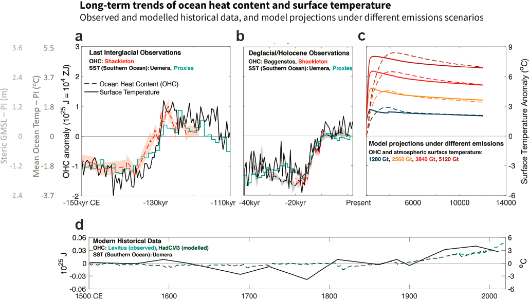
NOTES: (a) Penultimate glacial to Last Interglacial interval (Shackleton et al., 2020). (b) Last glacial interval to modern interglacial (Baggenstos et al., 2019; Shackleton et al., 2019). (a-b) Antarctic ice core rare gas measurements provide estimates of past globally integrated OHC on the leftmost axis (dashed lines in a and b), which is scaled at left to global mean ocean temperature anomalies (°C) and to thermosteric component of global mean sea level (GMSL, m). OHC correlates closely to Southern Ocean sea surface temperatures (solid lines in a and b) from proxies in sediment cores and from ice core deuterium (Uemura et al., 2018). (c) Long-term projected (2000 to 12000 CE) future changes of OHC (dashed lines; left axis) and global average sea surface temperature (solid lines, right axis) in response to four greenhouse gas emissions scenarios (Clark et al., 2016). Projected future OHC are a similar scale as past changes in OHC on the scale of glacial–interglacial changes (dashed lines). (d) Model-simulated 1500–1999 OHC (Gregory et al., 2006) and 1955–2019 observations (Levitus et al., 2012). Recent (century-scale) OHC changes are two orders of magnitude less than the range exhibited during multimillennial glacial–interglacial oscillations. All data are expressed as anomalies relative to preindustrial time.
SOURCE: Fox-Kemper et al., 2021.
Southern Ocean surface temperatures from sedimentary core proxies (e.g., Sangiorgi et al., 2018; Shevenell et al., 2011; Uemura et al., 2018) are generally well correlated with global ocean temperatures (Baggenstos et al., 2019; Shackleton et al., 2019, 2020) because of the near conservative transport of heat across the ACC along density surfaces (Marshall and Speer, 2012). However, paleoceanographic records of global ocean heat content show much larger changes: about 2°C to 3°C across the last two glacial–interglacial transitions (Baggenstos et al., 2019; Shackleton et al., 2000, 2019), although this may include non-temperature-related effects of the rare gas proxy (Pöppelmeier et al., 2023). A full mechanistic understanding of the linkage between global and Southern Ocean surface sea temperatures, and critically over what timescales it holds, remains a topic of open investigation. Thus, there is a need to study the Southern Ocean surface and subsurface ocean temperatures and global oceanic heat content both in modern processes and paleo records, which will require sediment coring and drilling, as well as geophysical survey capabilities.
WHAT PROCESSES WILL IMPACT ANTARCTIC SEA ICE EXTENT AND THICKNESS ON DECADAL TIMESCALES?
Antarctic sea ice coverage expands from a summer minimum area of about 3 million km2 in the summer to a maximum of about 19 million km2 in September—among the largest seasonal changes on Earth. Because of the strong seasonality of sea ice, as well as its sensitivity to wind forcing and ocean–ice–atmosphere interactions, sea ice provides perhaps the most conspicuous example of climate variability in the Antarctic. As such, sea ice can indicate changes in atmospheric and oceanic mechanical and thermodynamic forcing and simultaneously impact atmospheric and oceanic variability through its role as mediator of air–sea heat and freshwater exchange. For example, sea ice not only plays an important role in the physical buttressing of ice shelves (Chapter 3), but also impacts the ocean’s global overturning circulation; sets heat and freshwater budgets (e.g., Abernathey et al., 2016; Haumann et al., 2016; Pellichero et al., 2018); and exerts control on primary productivity (e.g., Arrigo et al., 1997), the carbon cycle (e.g., Fogwill et al., 2020), and low-level clouds (e.g., DuVivier et al., 2021).
Circumpolar sea ice extent increased modestly starting in 1979, the beginning of the modern satellite record, until reaching successive record maxima in 2012–2015 (Reid et al., 2016). However, recent years (2016–present) have been characterized by extreme negative anomalies in sea ice extent, including the three lowest summer minima on record. This is particularly important because loss of sea ice exposes much of the coastline and ice shelves to open ocean. This recent spate of anomalously low sea ice culminated in the ongoing dramatic reduction of sea ice in the austral winter of 2023, with sea ice more than 2 million km2 below normal (Figure 4-4). It is unknown if these recent changes are attributable to natural variability or mark a transition to a new sea ice state. A variety of proxy evidence, including early satellite data, whaling records, glacial ice core proxies, and statistical reconstructions from other climate variables, suggest that sea ice might have had substantially greater extent in the decades preceding the modern satellite record (Fogt et al., 2022; Hobbs et al., 2016; Maksym, 2019). This longer-term variability is also not captured in climate models (Hobbs et al., 2016). Additionally, the positive trend in sea ice between 1979 and 2015 contrasted with a predicted decrease in sea ice extent, as simulated by climate models (Roach et al., 2020). These discrepancies suggest that there may be processes that are not adequately understood or represented in models and that they may lead to unexpected variability in future trends.
These circumpolar trends can obscure the fact that sea ice variability is strongly regional, with often opposing trends or anomalies seen in different sectors (e.g., Stammerjohn et al., 2012) (Figure 4-5). It is well established that the proximate driver of sea ice variability is wind (e.g., Holland and Kwok, 2012) and that this driver is strongly connected to large-scale modes of climate variability (Eayrs et al., 2021; Hobbs et al., 2016; Stammerjohn et al., 2012). These modes include both local atmospheric variabilities, as embodied in the Southern Annular Mode, and tropical teleconnections,9 such as the El Niño–Southern Oscillation, but these teleconnections do not explain all observed trends (Hobbs et al., 2016). Various potential mechanisms have been suggested for the 1979–2015 increase, including growing freshwater input from the continental margins, changes in upper-ocean stratification, tropical climate variability, and ocean feedbacks initiated by wind-driven trends (Bintanja et al., 2013; Goosse and Zunz,
___________________
9Teleconnection refers to the relatedness of climate anomalies that are separated by large distances.
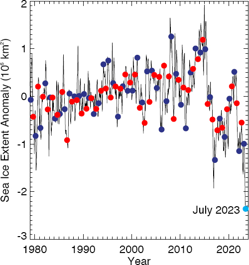
NOTES: Red dots show September (when ice is at maximum extent) monthly anomalies; blue dots show March (minimum extent) monthly anomalies. The cyan dot indicates the extreme record low anomaly for 2023 for the last month for which data were available at the time of writing of this report (July 2023).
SOURCE: Data from DiGirolamo et al., 2022; Meier et al., 2023.
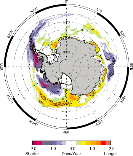
NOTES: Sea ice duration is defined as the period over which an area remains ice covered in winter (following Stammerjohn et al., 2008). Areas enclosed in black contours denote where trends are significant at the 95 percent level.
SOURCE: Data from DiGirolamo et al., 2022; Meier et al., 2023.
2014; Holland et al., 2018; Lecomte et al., 2017; Meehl et al., 2016). Likewise, the dramatic switch to record low ice extent has been attributed to a combination of anomalous atmospheric circulation, changes in ocean heat transport, atypical storminess, and changes in winter preconditioning of the upper ocean (Schlosser et al., 2018; Stuecker et al., 2017; Turner et al., 2020). Observational studies underpinning these processes are lacking. Untangling the connections between large-scale modes of climate variability, anthropogenic forcing, and the role of ice–atmosphere–ocean drivers and feedbacks will require both process-level observations and widespread, sustained monitoring efforts.
In contrast to the Arctic, upper-ocean stratification in the Antarctic is weak (Maksym, 2019). As a result, dense water (which is released when sea ice forms) sinks and entrains the warm deep waters below into the mixed layer, limiting ice growth and even melting ice in midwinter (Martinson, 1990). Hence much of the sea ice cover in the Antarctic is thin (Worby et al., 2008). Modeling suggests that sustained anomalous ice growth and buildup of subsurface heat may trigger enhanced mixing and destabilization of the upper ocean, as well as deeper convection, thereby reducing ice thickness and extent. In contrast, enhanced ice melt stabilizes the water column and limits mixing of subsurface heat, leading to increased ice extent (Lecomte et al., 2017; Zhang et al., 2019). This weak ocean stratification contributes to dramatic deep convection in the Weddell Sea Polynya, a vast area of open water within the Weddell Sea winter sea ice cover that appeared in the mid-1970s and again in 2016 (Campbell et al., 2019; Vernet et al., 2019). On seasonal timescales, ice–ocean processes—such as seasonal ice–ocean albedo (Stammerjohn et al., 2012), mesoscale ice–edge interactions (Gupta et al., 2020), and storm–ice–ocean interactions (Kohout et al., 2014; Turner et al., 2020)—all contribute to sea ice variability. There are a few integrated process-based observations at the spatial and temporal scales that are needed to understand how these ice–ocean interactions and feedbacks may play a role in past and future variability in the sea ice cover.
Ice thickness remains the most critical unknown of Antarctic sea ice. Sea ice thickness and its distribution control the exchange of energy and momentum between the ocean and atmosphere, water mass transformation, CO2 and other gas exchange, light availability for primary production under the ice, and the dynamics of the ice itself. Perhaps most critically, ice thickness (and to a lesser degree snow cover, which is also poorly constrained) determines the transport of freshwater via ice drift in the Southern Ocean, with a net transport of freshwater from southern to northern waters. Variability in this transport has increased in recent decades (Haumann et al., 2016), with significant consequences on the global climate through its impact on vertical exchange of ocean heat and carbon.
Observations are needed to determine the controls on sea ice extent and thickness, including ice–ocean fluxes for heat and salinity, as well as the snow and ice thickness of sea ice during its production in polynyas and after-wards as it drifts and deforms. Satellite altimeter observations are the only practical means of obtaining year-round circumpolar observations. Even when in situ sea ice thickness measurements are taken, they may be biased to thinner and less deformed areas that icebreakers can access. However, satellite observations carry uncertainties, as they do not provide a direct measurement of ice thickness and ice characterization. In fact, circumpolar satellite–derived ice thicknesses can be as much as twice as thick as in situ estimates (Kacimi and Kwok, 2020). The upcoming NISAR10 mission, as well as future higher-resolution passive microwave and altimeter missions, may increase opportunities for in situ validation, improved high-resolution imagery for ice conditions, and large-scale ice drift and deformation; these observations may reduce some of the aforementioned uncertainties.
Despite the need for in situ validation of satellite measurements, few of these measurements have been obtained. In situ ice measurements are hampered by both access to and logistical difficulties in measuring thicker ice. While new modalities for autonomous observations and deployment of platforms are emerging, icebreaker support is still required for almost all in situ observations of ice cover at present and for the foreseeable future. Deep-winter ice pack access has previously only been possible in early winter with the Nathaniel B. Palmer. Improved in situ observations will require greater access to regions of thicker ice, which can be afforded by a Polar Class 3 vessel. Access to the ice is necessary for most sea ice studies, including sampling, observation, and deployments. Ice stations11 have been a mainstay of sea ice–based survey and process observations. These studies require the capability to easily deploy personnel and equipment directly via gangway and a crane-deployed person basket.
___________________
10NISAR is the NASA-ISRO (Indian Space Research Organization) Synthetic Aperture Radar.
11Ice Stations allow personnel and equipment to access ice floes and are a standard observation strategy for taking ship-supported, on-ice measurements over periods of hours to weeks.
The spatial and temporal reach of vessels can be extended by a variety of autonomous platforms. These platforms allow for time-series observations at various spatial scales of ice growth, production, melt, and deformation, coupled with atmospheric and upper-ocean profiling and fluxes. The suite of ocean- and ice-based platforms includes wave and deformation buoy arrays, ice mass balance buoys, ice stations, GPS drifters, atmosphere ocean-flux buoys, ice-tethered platforms, ice-capable BGC-Argo floats, and moored devices with upward-looking sonars. Under the ice, gliders and medium- to long-range AUVs can provide measurements of coupled ice thickness and upper-ocean properties. The deployment of these instruments currently relies on icebreaker access into the sea ice. However, as technological developments in sensors, vehicles, and buoy modalities evolve, observations can be deployed far from a vessel, or from aircraft or coastal stations. Such advances are expected to include platforms that can be deployed remotely by UAS or AUV, survive freeze-up and melt, and provide on- and off-shelf operation and improved positioning under ice. Advances may also include long-range AUVs and gliders that have improved under-ice and environment-aware navigation, obstacle avoidance, and onboard adaptive mission planning. Such developments are needed to extend the reach (both spatially and temporally) of icebreakers and to provide widespread spatiotemporal observations of the ice, atmosphere, and ocean across large spatial scales and across seasons.
Fixed-wing aircraft, helicopters, and UASs can enable measurements of ice–ocean fluxes and ice thickness and drifting through a suite of lidar, radar, and electromagnetic measurements (e.g., Haas et al., 2010). UAS-supported measurements are more economical than measurements from crewed aircraft, but they are unlikely to supplant crewed aircraft for large-scale surveys in the near term. Future developments in observational systems may permit widespread deployment of miniaturized platforms by UAS, while future developments in long-range, heavy-lift UASs may also allow for a broad array of future ice and ocean observational systems. More traditional airborne support also enables deployment of observation systems. Currently, helicopter support is the most expedient means of deploying ice-tethered platforms and buoy arrays in areas that vessels may not be able to reach.
CONCLUSIONS
Climate change is expected to have significant social, economic, and health impacts on both national and global populations. The global ocean has so far absorbed more than 90 percent of the excess heat from humanity’s input of greenhouse gases to the atmosphere (two-thirds of that in the waters from the Southern Ocean), thus mediating the rate of global atmospheric warming. The Southern Ocean plays an outsized role in this global climate system, as most deep waters rise to the surface and exchange heat and carbon with the atmosphere in this area. It also serves as a crossroads, connecting the circulation of all ocean basins and controlling the strength and properties of the global deep overturning circulation through the production of AABW, as well as shallower intermediate and mode waters that impact lower latitudes. Large changes in the lower limb of the overturning circulation have been documented in paleoceanographic records and implicated in the release to the atmosphere of CO2 stored in the deep ocean. However, variability and rates of change of this lower limb of the overturning circulation are poorly understood and sparsely measured, compared with those of the upper ocean.
Conclusion 4-1: Additional sediment coring and drilling, as well as deployment of autonomous platforms, are needed to understand the role of the Southern Ocean in controlling the variability of the global overturning circulation and its long-term influence on total oceanic heat content, carbon storage, and climate.
Given that the Southern Ocean is responsible for about 40–50 percent of the net removal of fossil fuel CO2 emissions, there is a need to better constrain how its carbon reservoir may change. Prediction of these changes will benefit from an improved understanding of the physical processes that control the large-scale (hundreds of kilometers) distributions of heat, carbon, and nutrients. Notably, these distributions often depend on circulation features and air–sea interactions at smaller spatial scales (100 m to 100 km).
Conclusion 4-2: Collecting biogeochemical and physical oceanographic data from crewed and uncrewed vehicles at temporal and spatial scales reflective of the dominant scales of physical variability in the upper ocean, including mesoscale and submesoscale variations, will improve constraints on air–sea exchange and the Southern Ocean’s contribution to future atmospheric concentrations of carbon dioxide.
A priority identified in both Chapters 3 and 4 is to improve constraints on the oceanic transport of heat toward the Antarctic coast and the oceanic thermal forcing of Antarctic ice shelves. This is essential to project not only future sea level rise but also the strength of the lower limb of the global overturning circulation and carbon sequestration in the ocean. A picture of interannual variations in heat transport has started to develop, but it remains difficult to assess this variability in the context of a full seasonal cycle. Observations of this heat flux are needed in the following locations: (1) at the continental shelf break, focused on transport within bathymetric troughs; (2) at the termini of floating ice shelves, with a spatial resolution sufficient for estimating transport into ice shelf cavities; and (3) at the ocean–ice interface within ice shelf cavities, with a particular focus near the grounding zone.
Conclusion 4-3: Sustained observations of a full seasonal cycle, carried out over multiple years, are needed to improve understanding of seasonal to interannual variations in the ocean’s density structure, heat delivery into Antarctic ice shelf cavities, and the production of Antarctic Bottom Water, which control the strength and structure of the global overturning circulation and rates of carbon sequestration in the ocean.
The sea ice–ocean system has seen recent dramatic variability and a possible regime shift in sea ice extent. The drivers of this variability and trend are poorly understood. Sea ice in the Southern Ocean is a sensitive indicator of change and is known to modulate freshwater fluxes and air–sea heat and carbon exchange; yet large biases still persist in model representations of sea ice extent. This suggests that key processes are not yet understood or represented in models.
Conclusion 4-4: Multiplatform and multiprogram initiatives that can cover a broad range of spatial and temporal scales will provide better understanding of controls on sea ice extent, as well as its role in air–ocean interaction, freshwater exchange, circulation dynamics, and carbon cycling.
TABLE 4-1 Science Traceability Matrix
| Science priority | Observations | Needed capability |
|---|---|---|
| What determines the net uptake and release of carbon dioxide (CO2) in the Southern Ocean and how will it change in the future? | Monitoring upper-ocean physical and biogeochemical properties, such as surface temperature, mixed-layer depth, stratification, pH, alkalinity, and surface partial pressure of CO2 | Icebreaker well equipped for diverse physical and biogeochemical ocean and atmospheric observations throughout the year in Antarctic coastal and offshore waters |
| Sustained observations, such as profiling moorings or cabled observatories | ||
| Ice-capable floats and gliders, equipped with biogeochemical sensors, capable of sampling both on and off the continental shelf and under sea ice |
| Science priority | Observations | Needed capability |
|---|---|---|
| What are the key temporal and spatial scales of upper-ocean processes that influence air–sea exchange? | Measurements of spatially localized and intermittent fluxes | Heterogeneous arrays of autonomous vehicles (e.g., Wave Gliders, Saildrones) and Lagrangian floats with environmental-sensing payloads, including scientific echosounders |
| Icebreaker-based capabilities for water collection for chemical and biological sampling and rapid underway sampling | ||
| Global measurements of surface heat and momentum fluxes | Multiple satellite missions (e.g., sea surface height from both radar and laser altimeters, surface temperature, ocean color) | |
| Surface momentum and heat fluxes | ||
| What are the pathways of ocean heat and biogeochemical properties between the open Southern Ocean and the Antarctic coast? | Sustained, year-round observations (e.g., temperature, salinity, surface heat/freshwater/momentum fluxes, trace elements) near the coast/ice shelf in coastal polynyas, in the ice shelf cavity, and near the grounding line | Icebreaker profiling, sampling, and instrument deployment |
| Autonomous vehicles with under-ice capabilities, environment-aware mission planning, and navigation | ||
| Low-maintenance, persistent observing systems (e.g., inexpensive moorings or cabled observatories) that provide full-year coverage of key heat flux choke points | ||
| Development of new surface flux sensors on satellites | ||
| Observations collected across a broad range of scales to track nonlocal responses | Collaborative efforts with international partners | |
| Airborne hydrographic surveys enabled by helicopters, planes, or uncrewed aerial systems | ||
| How can understanding past changes in the Southern Ocean heat and CO2 budgets elucidate the future? | Geochemical and paleontological proxies of past heat and carbon budgets and tracers of ocean circulation | Sediment coring and drilling from icebreaker |
| Geophysical survey capabilities (hull-mounted and towed) on icebreaker | ||
| What processes will impact Antarctic sea ice extent and thickness on decadal timescales? | Measurements of sea ice thickness, extent, and dynamics; ice–ocean fluxes (heat and salinity) at various spatial scales | Icebreaker that supports access to the ice, freezer lab facilities, and deployment of autonomous platforms both above and below the ice |
| Underway observations (e.g., conductivity temperature and depth systems, ship-mounted electromagnetic thickness measurements, photogrammetry, lidar) | ||
| Suite of ocean- and ice-based platforms (e.g., wave and deformation buoy arrays, ice mass balance buoys, ice stations, GPS drifters, atmosphere–ocean flux buoys, moored upward-looking sonars, ice-tethered platforms, ice-capable biogeochemical Argo (BGC-Argo) floats, moorings, gliders and autonomous underwater vehicles) | ||
| Satellite altimeter and synthetic aperture radar observations with increased spatial and temporal resolution | ||
| Airborne support for deployment and lidar, radar, and electromagnetic measurements |


