
A Viscous Multiblock Flow Solver for Free-Surface Calculations on Complex Geometries
G.Cowles, L.Martinelli (Princeton University, USA)
1 Introduction
The last two decades have brought about many major advances in the ability to predict the steady flow about an advancing ship. Solvers based on several formulations have been developed and validated using experimental data from well known ship forms. Experience has shown that in order to correctly predict the drag of even simple hulls at realistic Froude numbers, the surface cannot be linearized. That is, the dynamic and kinematic conditions must be applied to the fully deformed boundary giving a fully nonlinear update of the free surface. Also, while solution of the inviscid equations can efficiently predict the effects of altering hullform coefficients, in order to accurately predict the total drag, the interaction between the free surface and the viscous layer must be accounted for. This can be done by solving the full Reynolds averaged Navier Stokes equations (RANS) in the entire flowfield in conjunction with a proper model for the eddy viscosity. Lastly, in order to be useful within the time constraints of a typical design schedule, the run time of the solver must be on the order of several hours.
Several of the higher order domain methods include all the necessary aspects described above. However, the quality of the mesh has a large effect on both the convergence and accuracy of these methods. Realistic hullforms can be considerably more complicated than the Wigley hull. Fully appended sailboats and submarines as well as naval combatants with transom sterns give rise to topological constraints which can make it difficult, if not impossible for the grid generator to produce a high quality single block mesh with spacing suitable for Navier Stokes calculations. One solution to this problem is to eliminate the constraints of mapping a single Cartesian domain to the hull by using an unstructured mesh. However the successive generation of high quality, three dimensional unstructured meshes necessary to follow the deformation of the free surface is very expensive and complicated. Also, even with an efficient implementation, the flow solver is only about half as computationally efficient when compared with a structured solver with equal resolution. An alternative route to the improvement of grid quality is to use a multiblock implementation. It can provide exceptional topological flexibility which facilitates a more efficient placement of points as well as smooth the skewness of cells and gradients in spacing.
We decided that in order to begin making routine calculations on realistic ship geometries with run times suitable for use in a design process, a parallel, multiblock implementation was necessary. The strategy was to maintain as many elements of the efficient single processor cell-vertex based solver that was already in place. This vertex formulation [9] had benefitted from several developments. Excellent convergence rates were obtained by using multigrid acceleration, local time stepping, and residual smoothing in the bulk flow. Accuracy stemmed from the utilization of limiters in the free surface dissipation as well as the incorporation of a fully nonlinear free surface boundary condition. As an intermediate step towards our goal, a single block, parallel version of the solver was developed. This required a change from the cell-vertex stencil to a cell-center. This was because in the method of domain decomposition, a cell-vertex scheme requires processors to share flow field values at subdomain faces which can lead to difficulties with implementation at the interface. Details of the method as well as some results can be found in [17]
Once that was in place, a parallel, multiblock version was implemented in which viscous terms as well as a turbulence model are included. The multiblock strategy has only minimal effect on the efficiency of the code. Thus, similar to the single block, parallel version, inviscid flow solutions are achieved in minutes on eight processors. Due to the increased number of grid points, reduced time step, and added work in calculating the viscous terms, solutions of the Navier Stokes equations require a factor of 20 increase in CPU time over
the inviscid case. Thus, converged NS runs require about three hours on eight processors.
The establishment of an efficient baseline multiblock flow solver is extremely important because it enables both sea-keeping analysis and optimization to become practical tools in the design process.
2 Mathematical Models
For a viscous incompressible fluid moving under the influence of gravity, the differential form of the continuity equation and the Reynolds Averaged Navier-Stokes equations (RANS) in a Cartesian coordinate system can be cast, using tensor notation, in the form,

Here, ![]() is the mean velocity components in the xi direction,
is the mean velocity components in the xi direction, ![]() the mean pressure, and
the mean pressure, and ![]() the gravity force acting in the i-th direction, and
the gravity force acting in the i-th direction, and ![]() is the Reynolds stress which requires an additional model for closure. For implementation in a computer code, it is more convenient to use a dimensionless form of the equation which is obtained by dividing all lengths by the ship (body) length L and all velocity by the free stream velocity U∞. Moreover, one can define a new variable Ψ as the sum of the mean static pressure P minus the hydrostatic component −x3Fr−2. Thus the dimensionless form of the RANS becomes:
is the Reynolds stress which requires an additional model for closure. For implementation in a computer code, it is more convenient to use a dimensionless form of the equation which is obtained by dividing all lengths by the ship (body) length L and all velocity by the free stream velocity U∞. Moreover, one can define a new variable Ψ as the sum of the mean static pressure P minus the hydrostatic component −x3Fr−2. Thus the dimensionless form of the RANS becomes:
where ![]() is the Froude number and the Reynolds number Re is defined by
is the Froude number and the Reynolds number Re is defined by ![]() where ν is the kinematic viscosity, and is
where ν is the kinematic viscosity, and is ![]() a dimensionless form of the Reynolds stress.
a dimensionless form of the Reynolds stress.
Figure 1 shows the reference frame and ship location used in this work. A right-handed coordinate system Oxyz, with the origin fixed at the intersection of the bow and the mean tree surface is established. The z (x3) direction is positive upwards, y (x2) is positive towards the starboard side and x (x1) is positive in the aft direction. The free stream velocity vector is parallel to the x axis and points in the same direction. The ship hull pierces the uniform flow and is held fixed in place, ie. the ship is not allowed to sink (translate in z direction) or trim (rotate in x−z plane).
It is well known that the closure of the Reynolds averaged system of equation requires a model for the Reynolds stress. There are several alternatives of increasing complexity. Generally speaking, when the flow remains attached to the body,
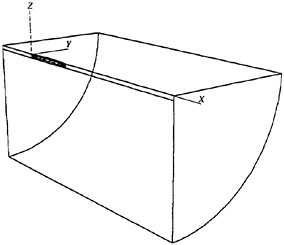
Figure 1: Reference Frame and Ship Location
a simple turbulence model based on the Boussinesq hypothesis and the mixing length concept yields predictions which are in good agreement with experimental evidence. For this reason a Baldwin and Lomax turbulence model has been initially implemented and tested [5]. On the other hand, more sophisticated models based on the solution of additional differential equations for the component of the Reynolds stress may be required. Notice that when the Reynolds stress vanishes, the form of the equation is identical to that of the Navier Stokes equations. Also, the inviscid form of the Euler equations is recovered in the limit of high Reynolds numbers. Thus, a hierarchy of mathematical model can be easily implemented on a single computer code, allowing study of the controlling mechanisms of the flow. For example, it has been shown in reference [9] that realistic prediction of the wave pattern about an advancing ship can be obtained by using the Euler equations as the mathematical model of the bulk flow, provided that a non-linear evolution of the free surface is accounted for. This is not surprising, since the typical Reynolds number of an advancing vessel is of the order of 108.
Free Surface Boundary Conditions
When surface tension as well as tangential stresses are neglected, the boundary condition on the free surface consists of two equations. The first, the dynamic condition, states that the pressure acting on the free surface is equal to the stresses normal to the free surface. It was found that the inclusion of the viscous stresses had little to no effect on the solution since they are of the order ![]() . Thus the dynamic condition that pressure is a constant is a good approximation. The kinematic condition states that the free surface is a material surface: once a fluid particle is on the free surface, it forever remains on the surface. The dynamic and kinematic boundary conditions may be expressed as
. Thus the dynamic condition that pressure is a constant is a good approximation. The kinematic condition states that the free surface is a material surface: once a fluid particle is on the free surface, it forever remains on the surface. The dynamic and kinematic boundary conditions may be expressed as
p=constant
(1)
where z=β (x, y, t) is the free surface location.
Hull and Farfield Boundary Conditions
The remaining boundaries consist of the ship hull, the meridian, or symmetry plane, and the far field of the computational domain. In the viscous formulation, a no-slip condition is enforced on the ship hull. For the inviscid case, flow tangency is preserved. On the symmetry plane (that portion of the (x, z) plane excluding the ship hull) derivatives in the y direction as well as the υ component of velocity are set to zero. The upstream plane has u=Uo, υ=0, w=0 and ψ=0 (p=−zFr−2). Similar conditions hold on the outer boundary plane which is assumed far enough away from the hull such that no disturbances are felt. A radiation condition should be imposed on the outflow domain to allow the wave disturbance to pass out of the computational domain. Although fairly sophisticated formulations may be devised to represent the radiation condition, simple extrapolations proved to be sufficient in this work.
For calculations in the limit of zero Froude number (double-hull model) the (z=0) plane is also treated as a symmetry plane.
3 Numerical Solution
The formulation of the numerical solution procedure is based on a finite volume method (FVM) for the bulk flow variables (u, υ, w and ψ), coupled to a finite difference method for the free surface evolution variables (β and ψ).
Bulk Flow Solution
The finite volume solution for the bulk flow follows the same procedures that are well documented in references [1, 2]. The governing set of differential flow equations are expressed in the standard form for artificial compressibility [6] as outlined by Rizzi and Eriksson [7]. In particular, letting w be the vector of dependent variables:
(2)
Here f, g, h and fv, gv, hv represent, respectively, the inviscid and viscous fluxes.
Following the general procedures used in the finite volume formulation, the governing differential equations are integrated over an arbitrary volume V. Application of the divergence theorem on the convective and viscous flux term integrals yields
(3)
where Sx, Sy and Sz are the projections of the area ∂V in the x, y and z directions, respectively. In the present approach the computational domain is divided into hexahedral cells. Two discretization schemes are considered in the present work. They differ primarily in that in the first, the flow variables are stored at the grid points (cell-vertex) while in the second they are stored in the interior of the cell (cell-center). While the details of the computation of the fluxes are different for the two approaches, both cell-center and cell-vertex schemes yield the following system of ordinary differential equations [4]
where Cijk and Vijk are the discretized evaluations of the convective and viscous flux surface integrals appearing in equation 3 and Vijk is the volume of the computational cell. In practice, the discretization scheme reduces to a second order accurate, nondissipative central difference approximation to the bulk flow equations on sufficiently smooth grids. A central difference scheme permits odd-even decoupling at adjacent nodes which may lead to oscillatory solutions. To prevent this “unphysical” phenomena from occurring, a dissipation term is added to the system of equations such that the system now becomes
(4)
For the present problem a fourth derivative background dissipation term is added. The dissipative term is constructed in such a manner that the conservation form of the system of equations is preserved. The dissipation term is third order in truncation terms so as not to detract from the second order accuracy of the flux discretization.
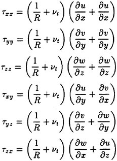
Discretization of the Viscous Terms
The discretization of the viscous terms of the Navier Stokes equations requires an approximation to the velocity derivatives ![]() in order to calculate the stress tensor. In order to evaluate the derivatives one may apply the Gauss formula to a control volume V with the boundary S.
in order to calculate the stress tensor. In order to evaluate the derivatives one may apply the Gauss formula to a control volume V with the boundary S.
where nj is the outward normal. For a hexahedral cell this gives
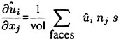
(5)
where ûi is an estimate of the average of ui over the face.
This technique requires motivates the introduction of dual meshes for the evaluation of the velocity derivatives and the flux balance as sketched for for the two dimensional case in figure 2.
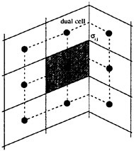
Figure 2: Viscous discretization for cell-centered algorithm.
Multigrid time-stepping
Equation 4 is integrated in time to steady state using an explicit multistage scheme. For each bulk flow time step, the grid, and thus Vijk, is independent of time. Hence equation 4 can be written as
(6)
where the residual is defined as
and the cell volume Vijk is absorbed into the residual for clarity.
The full approximation multigrid scheme of this work uses a sequence of independently generated coarser meshes by eliminating alternate points in each coordinate direction. In order to give a precise description of the multigrid scheme, subscripts may be used to indicate the grid. Several transfer operations need to be defined. First the solution vector on grid k must be initialized as
where wk−1 is the current value on grid k−1, and Tk,k−1 is a transfer operator. Next it is necessary to transfer a residual forcing function such that the solution grid k is driven by the residuals calculated on grid k−1. This can be accomplished by setting
where Qk,k−1 is another transfer operator. Then Rk (wk) is replaced by Rk (wk)+Pk in the time- stepping scheme. Thus, the multistage scheme is reformulated as

The result wk(m) then provides the initial data for grid k+1. Finally, the accumulated correction on grid k has to be transferred back to grid k−1 with the aid of an interpolation operator Ik−1,k. Clearly the definition of Tk,k−1, Qk,k−1, Ik−1,k depends on whether a cell-vertex or a cell-center formulation is selected. A detailed account can be found in reference [13].
With properly optimized coefficients, multistage time-stepping schemes can be very efficient drivers of the multigrid process. In this work we use a five stage scheme with three evaluation of dissipation [8] to drive a W-cycle of the type illustrated in Figure 3.
Figure 3: Multigrid W-cycle for managing the grid calculation. E, evaluate the change in the flow for one step; T, transfer the data without updating the solution.
In a three-dimensional case the number of cells is reduced by a factor of eight on each coarser grid. On examination of the figure, it can therefore be seen that the work measured in units corresponding to a step on the fine grid is of the order of
and consequently the very large effective time step of the complete cycle costs only slightly more than a single time step in the fine grid.
Free Surface Solution
Both a kinematic and dynamic boundary condition must be imposed at the free surface which require the adaption of the
grid to conform to the computed surface wave Since flow values are stored at cell centers, they must be extrapolated up one half cell for solution of the kinematic condition. By introducing a curvilinear coordinate system that transforms the curved free surface β (x, y) into computational coordinates β (ξ, η), equation 1 can be case in a form more amenable to integration. This results in the following kinematic condition:
(7)
Where U and V are the contravariant velocity components give by:
(8)
(9)
Figure 4 displays the computational stencil for the free surface update. It differs slightly from the bulk flow stencil, owing to velocity values held at the centers of the surface faces, while the free surface heights are held at surface vertices. The integration is a 3 stage Runge Kutta algorithm with dissipation evaluations on all stages.
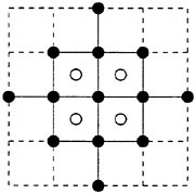
Figure 4: Free Surface Stencil
In our original method, equation 7 was augmented by high order diffusion [1, 2]. Such a scheme can be obtained by introducing anti-diffusive terms in a standard first order formula. In particular, it is well known that for a one-dimensional scalar equation model, central difference approximation of the derivative may be corrected by adding a third order dissipative flux:
(10)
where ![]() at the cell interface. This is equivalent to the scheme which we have used until now to discretize the free surface, and which has proven to be effective for simple hulls. However, on more complex configurations of interest, such as combatant vessels and yachts, the physical wave at the bow tends to break. This phenomenon cannot be fully accounted for in the present mathematical model. In order to avoid the overturning of the wave and continue the calculations lower order dissipation must be introduced locally and in a controlled manner. This can be accomplished by borrowing from the theory of non-oscillatory schemes constructed using the Local Extremum Diminishing (LED) principle [10, 11]. Since the breaking of a wave is generally characterized by a change in sign of the velocity across the crest, it appears that limiting the antidiffusion purely from the upstream side may be more suitable to stabilize the calculations and avoid the overturning of the waves [12]. By adding the anti-diffusive correction purely from the upstream side one may derive a family of UpStream Limited Positive (USLIP) schemes:
at the cell interface. This is equivalent to the scheme which we have used until now to discretize the free surface, and which has proven to be effective for simple hulls. However, on more complex configurations of interest, such as combatant vessels and yachts, the physical wave at the bow tends to break. This phenomenon cannot be fully accounted for in the present mathematical model. In order to avoid the overturning of the wave and continue the calculations lower order dissipation must be introduced locally and in a controlled manner. This can be accomplished by borrowing from the theory of non-oscillatory schemes constructed using the Local Extremum Diminishing (LED) principle [10, 11]. Since the breaking of a wave is generally characterized by a change in sign of the velocity across the crest, it appears that limiting the antidiffusion purely from the upstream side may be more suitable to stabilize the calculations and avoid the overturning of the waves [12]. By adding the anti-diffusive correction purely from the upstream side one may derive a family of UpStream Limited Positive (USLIP) schemes:
Where L (p, q) is a limited average of p and q with the following properties:
P1. L (p, q)=L (q, p)
P2. L (αp, αq)=αL (p, q)
P3. L (p, p)=p
P4. L (p, q)=0 if p and q have opposite signs.
It is well known that schemes which strictly satisfy the LED principle fall back to first order accuracy at extrema even when they realize higher order accuracy elsewhere. This difficulty can be circumvented by relaxing the LED requirement. Therefore the concept of essentially local extremum diminishing (ELED) schemes is introduced as an alternative approach. These are schemes for which, in the limit as the mesh width Δx → 0, maxima are non-increasing and minima are non-decreasing. In order to prevent the limiter from being active at smooth extrema it is convenient to set
where D (p, q) is a factor designed to reduce the arithmetic average, and become zero if u and v have opposite signs. Thus, for an ELED scheme we take
(11)
where
(12)
Properties P1–P3 are natural properties of an average, whereas P4 is needed for the construction of an LED scheme.
and ∈>0, r is a positive power, and s is a positive integer. Then D (p, q)=0 if p and q have opposite signs. Also if s=1, L (p, q) reduces to minmod, while if s=2, L (p, q) is equivalent to Van Leer’s limiter. By increasing s one can generate a sequence of limited averages which approach a limit defined by the arithmetic mean truncated to zero when p and q have opposite signs. These smooth limiters are known to have a benign effect on the convergence to a steady state of compressible flows. In comparison with experiment, it was found that the waterline profile calculated with ELED was more accurate when compared with LED or fourth differencing [17] [12].
Integration and Coupling with The Bulk Flow
The free surface kinematic equation may be expressed as
where Qij (β) consists of the collection of velocity and spatial gradient terms which result from the discretization of equation 7.
Once the free surface update is accomplished the pressure is adjusted on the free surface such that
The free surface and the bulk flow solutions are coupled by first computing the bulk flow at each time step, and then using the bulk flow velocities to calculate the movement of the free surface. After the free surface is updated, its new values are used as a boundary condition for the pressure on the bulk flow for the next time step. The entire iterative process, in which both the bulk flow and the free surface are updated at each time step, is repeated until some measure of convergence is attained: usually steady state wave profile and wave resistance coefficient.
This method of updating the free surface works well for the Euler equations since tangency along the hull can be easily enforced. However, for the Navier-Stokes equations the no-slip boundary condition is inconsistent with the free surface boundary condition at the hull/waterline intersection. To circumvent this difficulty the computed elevation for the second row of grid points away from the hull is extrapolated to the hull. Since the minimum spacing normal to the hull is small, the error due to this should be correspondingly small, comparable with other discretization errors.
4 Parallel Multiblock Implementation
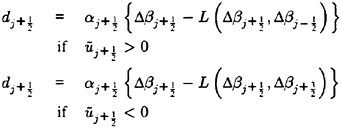
Topological constraints deriving from complex configurations necessitate the integration of a multiblock algorithm into the baseline code. An intermediate step was first taken in the form of a parallel, single block version of the code. Details of this method can be found in [17]. A multiblock strategy has been developed which requires minimum deviation from the parallel single block code. A halo is constructed around each block such that the flow solution within it is transparent to the block boundaries. Since both the convective and the dissipative fluxes are calculated at the cell faces (boundaries of the control volumes), all six neighboring cells are necessary, thus requiring the existence of a single level halo around each block. The dissipative fluxes are composed of third order differences of the flow quantities. Thus, at the boundary faces of each cell in the domain, the presence of the twelve neighboring cells (two adjacent to each face) is required. Figure 5 shows the neighboring cells which are required for the calculation of convective and dissipative fluxes. For each block, some of these cells will lie directly next to an interblock boundary. If the neighboring block is contained in a different processor, it will be necessary to pass the values across processors. With halos properly updated, the blocks
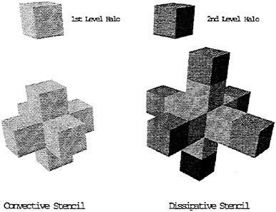
Figure 5: Convective and Dissipative Discretization Stencils.
are simply looped through the single block integrator. Thus, the highly optimized baseline code remains unchanged. The only difference in the integration lies in the implementation of the residual averaging. In the single block case, flow information from the processor’s entire subdomain is used for smoothing. In the multiblock case, only the information from the particular block being processed is utilized for this calculation. The converged solution remains unaffected and thus far, there has not been any significant effect in the rate of convergence.
Since the sizes of the blocks can be quite small, sometimes further partitioning severely limits the number of multigrid levels that can be used in the flows. For this reason, it was decided to allocate complete blocks to each processor.
The underlying assumption is that there always will be more blocks than processors available. If this is the case, every
processor in the domain would be responsible for the computations inside one or more blocks. In the case in which there are more processors than blocks available, the blocks can be adequately partitioned during a pre-processing step in order to at least have as many blocks as processors. This approach has the advantage that the number of multigrid levels that can be used in the parallel implementation of the code is always the same as in the serial version. Moreover, the number of processors in the calculation can now be any integer number, since no restrictions are imposed by the partitioning in all coordinate directions used by the single block program.
The only drawback of this approach is the loss of the exact load balancing that one has in the single block implementation. All blocks in the calculation can have different sizes, and consequently, it is very likely that different processors will be assigned a different total number of cells in the calculation. This, in turn, will imply that some of the processors will be waiting until the processor with the largest number of cells has completed its work and parallel performance will suffer. The approach that we have followed to solve the load balancing problem is to assign to each processor, in a pre-processing step, a certain number of blocks such that the total number of cells is as close as possible to the exact share for perfect load balancing.
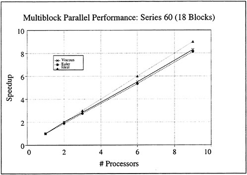
One must note that load balancing based on the total number of cells in each processor is only an approximation to the optimal solution of the problem. Other variables such as the number of blocks, the size of each block, and the size of the buffers to be communicated play an important role in proper load balancing, and are the subject of current study. Figure 20 shows speedups obtained on an 18 block mesh of Series 60 hull. One can see the good scalability of the method. The viscous speedups are closer to ideal due to increased granularity from the added work in calculating the viscous fluxes.
5 Results
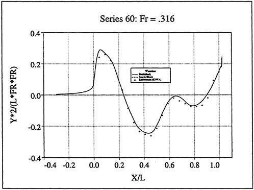
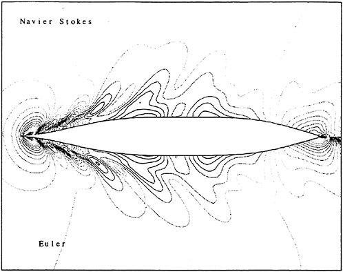
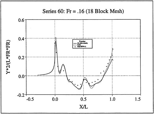
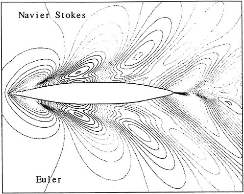
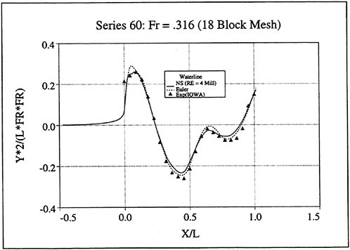
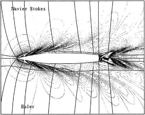
Figures 6 and 7 show overhead wave contours and waterlines for inviscid solutions of the Series 60 at a Froude number of .316. They serve to validate the multiblock code by comparison with both experiment and the previously developed single block parallel code. In order to validate the viscous solver, calculations were performed on the Series 60 hullform for comparison with the experimental data from Iowa [19]. Figures 8 and 9 show overhead wave contours and waterlines for both viscous and inviscid solutions of the Series 60 at Froude=.16. Figures 10 and 11 show wave elevation contours and waterlines for the Series 60 hull at Froude=.316. The Reynolds numbers for these calculations were 2 million and 4 million respectively, corresponding to the Iowa data. The grid spacing near the hull on the NS mesh is such that y+values in the first cell normal to hull reside in the range .75<y+<1.5.
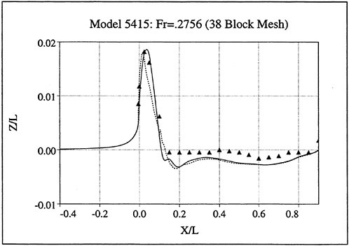
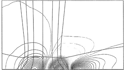
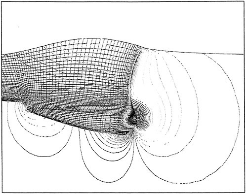
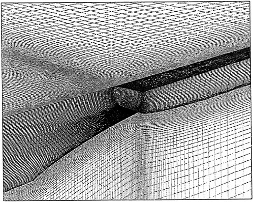
Figures 12 and 13 show overhead wave contours and waterlines for viscous and inviscid solutions of the model 5415 geometry at a Froude number of .2756 (20 Knots full scale). The Reynolds number was 12 million, corresponding to the test data taken at David Taylor Model Basin. Since the hullform has a transom stern, attempts to use a single structured block result in very skewed cells at the intersection of the and the symmetry plane aft of the boat. With a multiblock implementation however, a second block can be fitted to the transom and extended to the outflow plane. Figures 18 and 19 show details of the transom block as well as pressure contours on the sonar bulb.
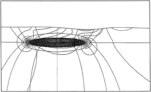
As a preliminary investigation of the application of our method to underwater vehicles, several calculations on a 6:1 ellipsoid were performed. A 1.25 million point mesh consisting of an inner O-H-O layer wrapped in an H-H-H shell was generated. The use of multiple layers facilitates adjustment of the spacing in the boundary layer without affecting the stretching in the far field. Figures 14 and 15 show pressure contours on the ellipsoid moving at a length-based Froude number of .62 and a depth/L of .18. The Reynolds number for this calculation was 4 million.
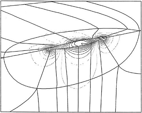
Initial analysis of an IACC racing yacht has also begun. Figure 16 displays the pressure contours on a double model IACC hull. The mesh topology is similar to the submarine. A O-H-O layer encompasses the hull while a H-H-H completes the far field. This topology was chosen because it will facilitate the addition of keel and rudder to the bare hull.
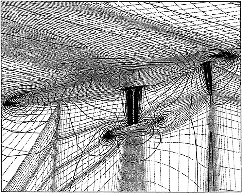
Figure 17 shows an inviscid single block solution on another IACC hull. One can see the highly skewed elements which result from using a single block on a fully appended hullform. Complex configurations such as this sailboat were a primary motivation for the implementation of multiblock.
Conclusion
A cell center, viscous, parallel multiblock version of the code has been developed and implemented. Inviscid flow solutions on the order of half an hour for a grid size of one million mesh points have been achieved on 16 processors of an IBM SP2. Viscous solutions on a mesh of same dimensions demand a factor of 5 increase in CPU work. Future efforts will concentrate on reducing the discrepancy in calculation time between the inviscid and viscous solutions. Progress towards improved dissipation and smoothing in the bulk flow to accelerate convergence has already begun. Additional speedup will be acquired by improving the pseudotime interaction between the bulk flow and the free surface; specifically at the intersection of the waterline and hull. Finally, a more realistic and robust turbulence model needs to be implemented. Even without these forthcoming improvements, however, the current version still provides turn-around times of 2 hours on 16 processors, rendering the Navier-Stokes solver suitable for utilization in design.
REFERENCES
[1] Farmer, J.R., Martinelli, L., and Jameson, A., “A Fast Multigrid Method for Solving the Nonlinear Ship Wave Problem with a Free Surface,” Proceedings, Sixth International Conference on Numerical Ship Hydrodynamics, pp. 155–172, 1993.
[2] Farmer, J.R., Martinelli, L., and Jameson, A., “A Fast Multigrid Method for Solving Incompressible Hydrodynamic Problems with Free Surfaces,” AIAA Journal, v. 32, no. 6, pp. 1175–1182, 1994.
[3] Jameson, A., “Optimum Aerodynamic Design Using CFD and Control Theory,” Proceedings, 12th Computational Fluid Dynamics Conference, San Diego, California, 1995
[4] Jameson, A., “A Vertex Based Multigrid Algorithm For Three Dimensional Compressible Flow Calculations,” ASME Symposium on Numerical Methods for Compressible Flows, Annaheim, December 1986.
[5] Baldwin, B.S., and Lomax, H., “Thin Layer Approximation and Algebraic Model for Separated Turbulent Flows,” AIAA Paper 78–257, AIAA 16th Aerospace Sciences Meeting, Reno, NV, January 1978.
[6] Chorin, A., “A Numerical Method for Solving Incompressible Viscous Flow Problems,” Journal of Computational Physics, v. 2, pp. 12–26, 1967.
[7] Rizzi, A., and Eriksson,L., “Computation of Inviscid Incompressible Flow with Rotation,” Journal of Fluid Mechanics, v. 153, pp. 275–312, 1985.
[8] Martinelli, L., “Calculations of Viscous Flows with a Multigrid Method,” Ph.D. Thesis, MAE 1754-T, Princeton University, 1987.
[9] Farmer, J., “A Finite Volume Multigrid Solution to the Three Dimensional Nonlinear Ship Wave Problem,” Ph.D. Thesis, MAE 1949-T, Princeton University, January 1993.
[10] A.Jameson, “Analysis and design of numerical schemes for gas dynamics 1, artificial diffusion, upwind biasing, limiters and their effect on multigrid convergence,” Int. J. of Comp. Fluid Dyn., To Appear.
[11] A.Jameson, “Analysis and design of numerical schemes for gas dynamics 2, artificial diffusion and discrete shock structure,” Int. J. of Comp. Fluid Dyn., To Appear.
[12] J.Farmer, L.Martinelli, A.Jameson, and G.Cowles, “Fully-nonlinear CFD techniques for ship performance analysis and design,” AIAA paper 95–1690, AIAA 12th Computational Fluid Dynamics Conference, San Diego, CA, June 1995.
[13] A.Jameson, “Multigrid algorithms for compressible flow calculations,” In Second European Conference on Multigrid Methods , Cologne, October 1985. Princeton University Report MAE 1743.
[14] L.Martinelli and A.Jameson, “Validation of a multigrid method for the Reynolds averaged equations,” AIAA paper 88–0414, 1988.
[15] L.Martinelli, A.Jameson, and E.Malfa, “Numerical simulation of three-dimensional vortex flows over delta wing configurations,” In M.Napolitano and F.Sabbetta, editors, Proc. 13th International Conference on Numerical Methods in Fluid Dynamics, pages 534–538, Rome, Italy, July 1992. Springer Verlag, 1993.
[16] F.Liu and A.Jameson, “Multigrid Navier-Stokes calculations for three-dimensional cascades,” AIAA paper 92–0190, AIAA 30th Aerospace Sciences Meeting, Reno, Nevada, January 1992.
[17] G.Cowles, and L.Martinelli “Fully Nonlinear Hydrodynamic Calculations for Ship Design on Parallel Computing Platforms,” Proc. 21st International Symposium on Naval Hydrodynamics, Trondheim, Norway, June 1996
[18] G.Cowles, and L.Martinelli “A Cell-Centered Parallel Multiblock Method for Viscous Incompressible Flows with a Free Surface,” Proc. 13th AIAA Computational Fluid Dynamics Conference, Snowmass, Colorado, July 1997
[19] Y.Toda, F.Stern, and J.Longo “Mean-Flow Measurements in the Boundary Layer and Wake and Wave Field of a Series 60 Cb=.6 Ship Model for Froude Numbers .16 and .316 IIHR Report No. 352, Iowa Institute of Hydraulic Research, August 1991
DISCUSSION
H.Haussling
Naval Surface Warfare Center, Carderock Division, USA
The authors have demonstrated what appears to be a very efficient, parallel code for obtaining free-surface RANS solution. However, the results presented for Model 5415 indicate that the code is predicting a dry transom when measured data and other RANS computations indicate a wet transom. One possible explanation for this is that the solution is missing a significant part of the slowing of the flow in the boundary layer. Such a bias would lead to higher than realistic velocities near the transom and hence a solution behavior more like a higher speed than that being run.
DISCUSSION
H.Raven
Maritime Research Institute, The Netherlands
I am interested in the flow off the transom shown in Fig. 12. In your presentation, the transom appeared to be dry. Does this agree with the experiment at this speed? What happens if you reduce the speed in your calculation (Euler and RANS)?
AUTHORS’ REPLY
The dry transom is a result of the mesh treatment at the stern of the ship. At low speeds, the flow aft of the transom has a slight unsteady character. The viscous terms and turbulence model have been validated in several applications.2,3 The main intention of the current work is to focus on schemes which capture the detailed wave structure at a range of Froude numbers. In order to focus on the free surface, a steady velocity field must be provided. When the study is completed, the full approximation will resume.
DISCUSSION
R.Lohner
George Mason University, USA
This is a very impressive piece of work, combining:
-
Advanced finite volume solvers for the incompressible RANS equations with fully nonlinear free surface boundary conditions;
-
Efficient multigrid acceleration to steady state;
-
Multiblock spatial discretization to handle geometrical complexity;
-
Parallel computing; and
-
Validation through comparisons to experimental data.
As in any paper, there are some minor flaws that could be improved. Of these, the ones that I consider significant are as follows:
1. The statement that the generation of proper unstructured grids for free surface hydrodynamic problems is complicated and expensive is not true. One does not need to generate a new mesh as the solution evolves. All that is required is mesh movement. This distinction is not immediately evident for structured grids, but greatly facilitates the use of unstructured grids in this context. We refer the authors to the following two references:
Lohner, R., Yang, C., Onate, E. and Idelssohn, S. 1997 An Unstructured Grid-Based, Parallel Free Surface Solver. AIAA-97–1830.
Lohner, R., Yang, C. and Onate, E. 1998 Viscous Free Surface Hydrodynamics Using Unstructured Grids. Proc. 22nd Symp. on Naval Hydrodynamics.
(Bear in mind that the author uses unstructured grids routinely for these types of problems; i.e., take this comment with a grain of salt.)
2. The argument is made that multiblock grids reduce skewness, yet the mesh shown in Figure 17 shows a considerable degree of skewness. Perhaps one should say that the main advantage of multiblock is that it can discretize complex geometries where a uniblock approach is impossible.
3. For the Baldwin-Lomax model, are the normals forced to be aligned with (sometimes very curved) gridlines? If so, is this not highly inaccurate? If not, are the normals and their information passed across multiblock boundaries?
4. The section covering the results obtained using this method can be improved substantially. For example, any explanation why the RANS results in Figures 9, 11, 13 are just as good as the Euler results when compared to experiments? (Except for the first wave, which is always
improved with RANS due to the finer spacing normal to the wall). We have observed the same phenomenon for some of our calculations. Are the experiments flawed? Also, more discussion on gridsizes, convergence rates, timings, set-up times, etc.
Overall, an excellent piece of work. What next?
AUTHORS’ REPLY
-
The work time in the deformation of the structures grid is negligible relative to the calculation time. Following the fully deformed free surface mesh with an unstructured grid is considerably more complicated and somewhat more expensive. The statement in the paper was based on the author’s experience with 2-D unstructured methods for unsteady wave problems.1 However, having seen some of Professor Lohner’s work from the aeronautical side of his research regarding the motion of unstructured grids around twisting, falling, and exploding objects, I realize that his grid motion methods must be very efficient.
-
In regard to the comment that the mesh in Figure 17 is actually quite skewed; yes, it is. The intention of its inclusion in the paper was to show the difficulties that arise from using a single block topology mesh for a fully appended sailboat.
-
When generating the mesh, care is taken to maintain that the grid lines extend from the boat along the normal. In the turbulence model, distance from the wall is dotted with the normal. For our implementation, we feel that this is the best way to ensure that the resulting scheme follows the model as closely as possible to maintain accuracy. The information is not passed across block boundaries. Therefore care must be taken that the inner layer of blocks adjoining the hull completely include the boundary layer such that the eddy viscosity vanishes at the outer face.
-
There are some differences between the Euler and viscous waterlines due to differing velocity fields adjacent to the boat. The largest distinction is not displayed in the waterline comparisons but can be seen in the overhead comparisons. In the Euler case, the unphysical tangency condition imposed on the stern of these ships can cause the wave just aft of the transom to be much larger than the stern wave resulting from a viscous calculation.
Following the discusser’s advice, I will elaborate on some of the practical concerns of the code. The grid sizes for the three cases presented in this paper—the Series 60, Model 5415, and Elipsoid—are as follows: 920,000 pts (18 blocks), 1.1 million pts (38 blocks), and 1.3 million PTSA (44 blocks). A single node of an IBM SP2 requires a minute for one iteration of the Euler equations on a million point mesh. The calculations of the viscous fluxes require an additional 15% work. Speedups of over 8X have been obtained on 9 processors. The communication procedure is very fast; however, a proper load balance is important as well. In most cases, the deviation from exact balance does not exceed 5%. Euler calculations require about 350 iterations for convergence, while Navier Stokes require approximately double that number. Thus convergence of a viscous calculation can be achieved in a few hours. An inviscid flow solution on a one million point mesh is completed within an hour. However, this solution can be achieved using far fewer grid points. Setting up a calculation requires constructing a grid and running the preprocessor to set up the communication and boundary condition arrays for each processor. Grids are developed using Gridgen to define the boundaries and an in-house solver for the interior points. They require anywhere between 2 days and a week to build. The preprocessor requires less than a minute to perform its duties.
References
1B.Liou, L.Martinelli, T.Baker, and A. Jameson, “Calculation of Plunging Breakers with a Fully Implicit Adaptive Method,” AIAA paper 98–2968, AIAA 29th Fluid Dynamics Conference, Albuquerque, NM, June 1998.
2Farmer, J.R., Martinelli, L., and A.Jameson, “Multigrid Solutions of the Euler and Navier-Stokes Equations for a Series 60 Cb=.6 Ship Hull for Froude Numbers 0.160, 0.220, and 0.316,” Proceedings, CFD Workshop Tokyo 1994, Tokyo, Japan, March 1994.
3Belov, A., “A New Implicit Multigrid-Driven Algorithm for Unsteady Incompressible Flow Calculations on Parallel Computers,” Ph.D. Thesis, MAE 1636-T, Princeton University, 1997.
Navier-Stokes Computations of Ship Flows on Unstructured Grids
T.Hino (Ship Research Institute, Japan)
Abstract
An unstructured grid method for simulating three-dimensional incompressible viscous flows is presented. The governing equations to be solved numerically are the Navier-Stokes equations with artificial compressibility. The spatial discretization is based on a finite volume method for an unstructured grid. Second order accuracy in space is achieved using a flux-difference-splitting scheme with the MUSCL approach for inviscid terms and a central difference scheme for viscous terms. Time integration is carried out by the backward Euler method. The linear system derived by the linearization in time is solved by the Gauss-Seidel iteration. For the analysis of high Reynolds number flows, the k-ω-SST two equation turbulence model is used. The turbulence equations are solved in a similar way as the Navier-Stokes equations. The computational results for viscous flows around ships demonstrate the capability of the method to simulate complicated flow fields with reasonable accuracy.
1 Introduction
Computational fluid dynamics (CFD) analysis is now being used as a practical tool to predict flows around complex configurations. However, as configurations become complex, the efforts required for grid generation increase greatly. This is particularly true in case that conventional structured grids which are based on regular arrays of hexahedral cells are used. One way to overcome this difficulty is the use of multiblock grids which consist of either overlapping or non-overlapping blocks of structured grids. In this case, both a grid generation code and a flow solver must be able to handle special procedures for multiblock boundaries.
The other way is unstructured grid methods (1, 2) which employ irregularly connected cells of various shapes. Unstructured grid methods offer greater flexibility for handling complex shapes than structured grid counterparts. Even though unstructured grid generation around a complex configuration is as difficult as structured grid generation, a flow solver can be simplified because all the topological informations are kept in grids.
Unstructured grid methods were developed initially for solving compressible inviscid flow equations (3). Then the methods have been extended to compute viscous flows. Incompressible flow solvers have also been developed based on a pressure correction method (4) or on an artificial compressibility method (5).
In the CFD applications for ship hydrodynamics, there are increasing needs for flow predictions around more complex configurations, because practical ships are usually equipped with stern appendages, a rudder and a propulsor. Therefore, a 3D unstructured grid Navier-Stokes solver is expected to be a powerful tool in practical ship hydrodynamics as well as in other fluid engineering fields.
Hino developed unstructured grid methods for 2D incompressible inviscid flows with a free surface (6) and for 2D turbulent free surface flows (7) using an artificial compressibility approach. For 3D, Löhner et al. (8) developed an unstructured grid Euler solver based on pressure correction approach and computed free surface flows around ships. Also, Hino (9) developed a 3D unstructured Navier-Stokes solver based on artificial compressibility method and applied it to viscous flow simulations around a ship. The present study is the improvement of the method in (9). The spatial discretization and the turbulence model are modified to enhance accuracy and robustness of the scheme.
In Section 2, the governing equations are given and the spatial discretization is described followed by the explanation of the time integration scheme. Then the boundary conditions for numerical computations are briefly shown and the turbulence model used is presented. In Section 3, the numerical results with the present method are shown for flows around a ship hull and a ship with a rudder configuration. Finally, the concluding remarks are given in Section 4.
2 Numerical Scheme
2.1 Governing Equations
The governing equations to be solved are the three-dimensional Reynolds averaged Navier-Stokes equations for incompressible flows. With the introduction of artificial compressibility, they are written
in a vector form as
(1)
where

is the vector of flow variables which consist of p, pressure and (u, v, w), the (x, y, z)-components of velocity. The inviscid fluxes e, f and g are defined as
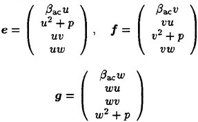
where βac is a parameter for artificial compressibility. ev, fv and gv are the viscous fluxes defined as
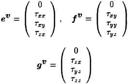
where
In the above expressions all the variables are made dimensionless using the reference density ρ0, velocity U0 and length L0. R is the Reynolds number defined as U0L0/ν where ν is the kinematic viscosity. νt is the nondimensional kinematic eddy viscosity determined by a turbulence model.
2.2 Spatial Discretization
(1) Finite volume formulation
Spatial discretization of the present scheme is based on a finite-volume method for an unstructured grid. Cell shapes the present solver can cope with are tetrahedron, prism, pyramid or hexahedron and face shapes are either triangular or quadrilateral as shown in Fig. 1.
These four types of cells give larger flexibility in handling complex geometries. In particular, it is suitable for a hybrid grid approach in which prisms and hexahedra are placed in the region close to a solid wall for the efficient resolution of boundary layers while tetrahedra and pyramids are used to tessellate the remaining region in a flexible manner. A cell centered layout is adopted which means flow variables q are defined at the centroid of each cell and a control volume is a cell itself. yields
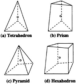
Fig. 1 Cell shapes.
Volume integration of Eq. (1) over a cell yields
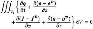
(2)
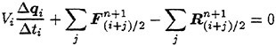
The first term in the integral can be expressed as the product of the cell volume Vi and the time derivative of the cell averaged value of flow variables qi, since the grid is stationary in the current applications. The remaining terms are converted into surface integration over cell faces using the divergence theorem. This yields the semi-discrete form of the governing equation as follows.
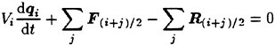
(3)
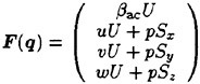
where i is a cell index and j is the index of next cells of the cell i. (i+j)/2 denotes the face between cells i and j as shown in Fig. 2
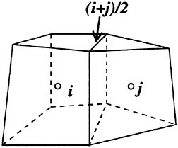
Fig. 2 Definition sketch of cell and face index.
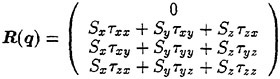
F and R are the inviscid and viscous fluxes defined as
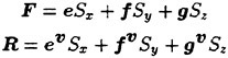
where (Sx, Sy, Sz) are the (x, y, z)-components of the area vector of a cell face in the direction from the cell i to the cell j.
(2) Discretization of inviscid fluxes
Components of the inviscid fluxes F are
where U=uSx+vSy+wSz. The inviscid fluxes are evaluated by the upwind scheme based on the flux-difference splitting of Roe (10). In the scheme, the numerical fluxes are computed as
(4)
where qR and qL are the flow variables on the right and the left sides of a cell face, respectively. |A| is defined in the following way. First, let A be the Jacobian of the inviscid flux F at a cell face:
where the flow variables at the cell face q(i+j)/2 are evaluated by the simple average of the right and the left side values, i.e.,
The eigenvalues of A are U, U, U+c, U−c where c is the pseudo-speed-of-sound defined as
By using the right-eigenvector R, A can be expressed as
where Λ is
Finally, |A| is given by
with
To achieve the second order accuracy in space, the MUSCL approach is used in which the flow variable q is reconstructed as a linear polynomial function inside each cell using the cell centroid values. Let the scalar quantity q be a component of q and q is assumed to be linearly varying in the vicinity of the cell i, i.e.,
(5)
where ∇qi=(∂qi/∂x, ∂qi/dy, ∂qi/∂z)T is the gradient of q at the cell i and xi is the coordinates of the cell centroid i. This equation is applied to the cell j which is adjacent to the cell i, which yields
or
A similar equation can be written for all the neighbor cells of i, thus,
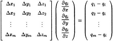
(6)
where
The above equation (6) gives the overdetermined system for ∇qi and the least squares solution can be obtained by solving it via QR decomposition. Finally, qR and qL are extrapolated using the gradient with the limiter function as follows
(7)
where x(i+j)/2 is the coordinates of the center of face (i+j)/2.
The limiter function Φ is used to enforce the monotonicity of the reconstruction. The form proposed by Barth (12) is used in the present scheme
which is written as
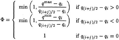
where qmax and qmm are the maximum and the minimum values of q at the cell i and its neighbors.
(3) Discretization of viscous fluxes
Viscous fluxes components are written as
The computation of R(i+j)/2 requires velocity gradient on a cell face. These are computed again by applying the divergence theorem to another control volume surrounding a cell face as shown in Fig. 3.

Fig. 3 Control volume for the evaluation of velocity gradient.
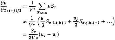
The values of q at the centroids i and j as well as at the nodes surrounding the face (i+j)/2 (k, k+1…) are used for the surface integration. For example, ∂u/∂x is computed as
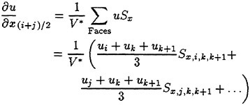
(8)
where V* is the volume of the current control volume and Sx,α,β,γ is the x-component of the outward area vector of the face formed by the nodes α, β and γ. This formulation is equivalent to centered differencing in the structured grid case and is second order accurate.
The velocity values at the nodes k, k+1 etc. are computed from the values at the cell centroids by the Laplacian weighted average (13) as follows
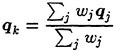
where the summation is for all the cells that share the node k. The weight wj is computed as
where λx, λy, λz are the solution of

with
This formulation gives the exact values for linearly varying functions and is second order accurate.
2.3 Time Integration
Since the artificial compressibility is introduced into the governing equations, incompressible flow fields can be obtained only as a steady state limit. Therefore, transient solutions are not physically valid. The time integration in the present scheme is thus the way to drive solutions to a steady state and time accuracy of the scheme is not important.
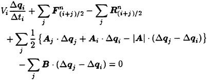
The first order backward Euler scheme is used for the time integration in which the governing equation is written as
(9)
where
and the superscripts denote the time step. Δti is time increment in local time stepping in which Δti is determined cell by cell in such a way that the CFL number is globally constant as follows
where CFL is the CFL number. The summation of the denominator is taken over all faces of the current cell.
The linearization of the inviscid flux Fn+1 with respect to time is made as follows
When the Jacobian ∂F/∂q is evaluated, the flux F is computed with the first order upwind scheme by setting

i.e., the inviscid flux is approximated by
Thus, ∂F/∂q · Δq is expressed as
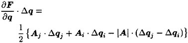
where
In the similar manner the viscous flux is linearized in time as
For the evaluation of the Jacobian ∂R/∂q, the velocity gradients are approximated by neglecting the contribution from the values at the nodes qk etc. That is, Eq. (8) is replaced by
where Sx is the area vector component of the face (i+j)/2 as defined earlier. Using the similar approximation for the other velocity gradients, R can be expressed as
where

with
Thus, ∂R/∂q · Δq becomes
Eq. (9) now becomes
(10)
The delta terms are rearranged into the form as follows
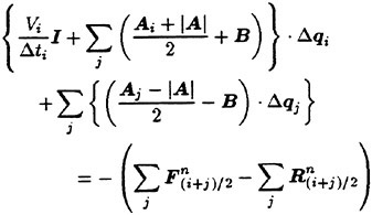
(11)
The equation above is a linear equation with respect to Δq. In order to solve this equation, the Symmetric Gauss-Seidel (SGS) iteration is adopted. To achieve fast convergence, the cells are ordered from upstream to downstream in the preprocessing stage. The Gauss-Seidel sweep is carried out from the upstream cell to the downstream first, then the second sweep follows in the reverse order. The following sweeps change the direction alternately.
2.4 Boundary Conditions
The cell faces on the boundaries are classified as the boundary faces. The boundary conditions
are implemented by giving the appropriate fluxes on the boundary faces based on the following conditions:
Solid wall:
Inflow:
Outflow:
Side:
Symmetry:
Symmetric Conditions
In case of the Dirichlet conditions, the fluxes can be computed using given values, while in case of the Neumann conditions, the flow variables on the face is set equal to those at the cell that contains the current face. In the time integration process, all the boundary conditions are treated implicitly.
2.5 Turbulence Model
A turbulence model is essential for simulating high Reynolds number flows of practical interests. There exist a number of turbulence models. They range from simple algebraic models or one- or two-equation models for the eddy viscosity concept to Reynolds stress models for the second order closure. However, no model has been proved to be universally applicable to general fluid engineering problems. In practice, a turbulence model must be selected based on the characteristics of a flow field of each problem. Ship flows, particularly stern flows, are extremely complicated, because they are essentially three dimensional separated flows with strong longitudinal vortices and free surface effects cannot be neglected in some cases. From the practical point of view, it is important that CFD computations can accurately simulate a propeller inflow, that is, a wake behind a ship hull. However, these extremely complicated ship flows are beyond the capability of most of existing turbulence models.
In the previous version of the present method (9), the Spalart-Allmaras one-equation model (14) is used as a turbulence model. Since the wake distribution for a tanker model simulated with the Spalart-Allmaras model showed poor agreement with the measurement (9), the k-ω-SST two-equation model by Menter (15) is newly adopted in the present scheme. This model uses the original k-ω model of Wilcox (16) in the inner region of the boundary layer and the standard k-∈ model in the other region in order to remove the dependence on the free stream condition of the original k-ω. The further modification which accounts for the effect of the turbulent shear stress transport is incorporated into the model. Since Deng et al. (17) showed that the original k-ω turbulence model well predicted the wake pattern behind a tanker hull, the present model is expected to work equally well for ship flows.
The model consists of the two transport equations, one for the turbulent kinematic energy k and the other for the turbulence frequency ω. The equations are written as
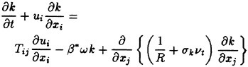
(12)
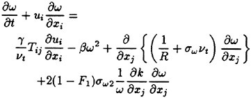
(13)
where Tij is the turbulent shear stress tensor defined as
The blending function F1 which is 1 in the inner region and 0 in the outer region is defined as follows;
with
where d is the distance to the closest wall and
The constant σk σω, β and γ are computed using the blending function F1 as
The constants for the inner region are based on the k-ω model with the modification for SST and are given as:
σk1=0.85, σω1=0.5, β1=0.0750, β*=0.09
The constants for the outer region come from the standard k-∈ formulation and these are:
σk2=1.0, σω2=0.856, β2=0.0828, β*=0.09
Finally, the turbulent kinematic eddy viscosity is computed by
where Ω is the magnitude of the vorticity and
The function F2 is given by
and
The boundary conditions for k and ω are as follows
Solid wall:
(where Δd is the distance to the centroid of the next cell from the wall)
Inflow:
Outflow:
Side:
Symmetry:
Symmetric Conditions
The numerical method employed for the solution of turbulent equations is similar to the one for flow equations except that the advection terms are evaluated by the first-order upwind scheme.
3. Results
3.1 A Tanker Hull
The first application is a three dimensional flow field around a ship hull form. A ship model is a VLCC hull with a bulbous bow called SR196A. The Reynolds number based on the length between perpendiculars Lpp is 4.0×10⁶ which corresponds to a model scale.
Fig. 4 Partial view of unstructured grid around a tanker hull.
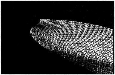
Fig. 5 Magnified view of grid at the bow.
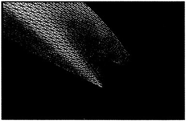
Fig. 6 Magnified view of grid at the stern.
The grid used is based on the 97×41×65 structured grid of O-O topology. The unstructured grid is generated from this grid by dividing all
the hexahedral cells of the structured grid into two prisms. The grid consists of 491,520 cells, 1,245,184 faces and 258,505 nodes. The partial views of the grid is shown in Fig. 4. Figs. 5 and 6 are the magnified views of the bow and stern regions, respectively Distributions of triangular faces on a body can be observed.
The computation starts using local time stepping with initial CFL of 10 and CFL is increased linearly up to 100 in the first 200 steps. The history of the total drag coefficient ![]() and the frictional drag coefficient
and the frictional drag coefficient ![]() where S is the wetted surface area is shown in Fig. 7. It is seen that the converged solution with engineering accuracy is obtained with about 1,000 iterations.
where S is the wetted surface area is shown in Fig. 7. It is seen that the converged solution with engineering accuracy is obtained with about 1,000 iterations.
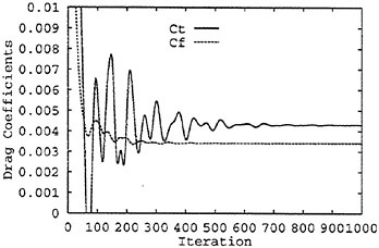
Fig. 7 History of drag coefficients.
Computed drag coefficients are shown in Table 1 together with the experimental data which is estimated as the form factor K=0.32 based on the Schoenherr friction line. The total drag is estimated by the present computation slightly lower than the experimental value while the frictional component agree well with the Schoenherr value.
Table 1. Drag coefficients of SR196A
|
|
Total Drag |
Frictional Drag |
|
Computed |
4.32×10⁻³ |
3.41×10⁻³ |
|
Experiment |
4.52×10⁻³ |
3.42×10⁻³ |
Computed pressure distributions on a ship hull and symmetric planes are shown in Figs. 8, 9 and 10. A high pressure zone at the bow and low pressure zones near the fore and aft shoulders can be seen. Also, low pressure regions appear at the bilge in the bow and the stern where streamlines turn around the bilge and velocity magnitude becomes large. These features off pressure distribution are typical for a ship of this kind.
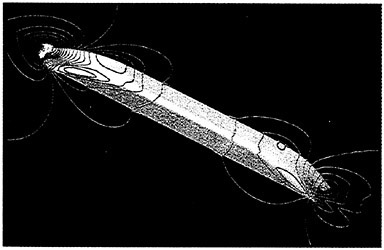
Fig. 8 Computed pressure distribution around a tanker hull.
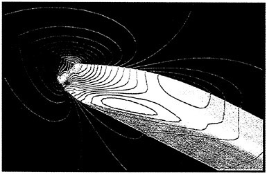
Fig. 9 Computed pressure distribution at the bow of a tanker hull.
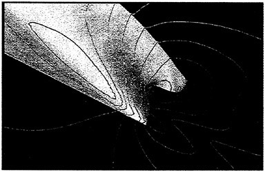
Fig. 10 Computed pressure distribution at the stern of a tanker hull.
For this hull, Suzuki et al. (18) measured velocity fields using a hot wire probe in a wind tunnel. Fig. 11 and Fig. 12 show the comparison of the computed velocity distributions with the measured data.
Fig. 11 shows the data at S.S. 1/2. In the measurement, the swirling motion can be seen in the region close to the keel where the axial velocity is small. The present computation reproduces this phenomenon although the extent, is smaller than the measurement.
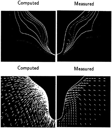
Fig. 11 Velocity distributions at S.S. 1/2. Axial velocity contours and crossflow vectors: present computation (left) and measurement (right) (18).
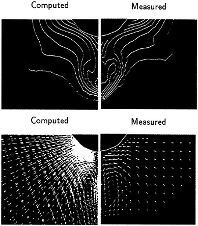
Fig. 12 Velocity distributions at S.S. 1/8. Axial velocity contours and crossflow vectors: present computation (left) and measurement (right) (18).
In Fig. 12 the velocity distributions at S.S. 1/8 is shown. The measured wake contour shows the so-called ‘hook’ shape which corresponds to the strong longitudinal vortex. The computed velocity distribution agrees reasonably well with the measurement. The ‘hook’ shape of the contour line is reproduced to some extent and the locations of vortex core are in good accordance with the measurement, although the computed result is still too diffusive. Fig. 13 shows the result with the Spalart-Allmaras turbulence model which is computed by the method described in (9) using the structured grid of 113×41×41 points. It is seen that the ‘hook’ shape is not simulated well with this model. The performance of the present k-ω-SST turbulence model is almost the same as the original k-ω model used by Deng et al. (17).
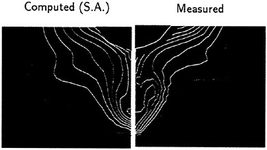
Fig. 13 Velocity distributions at S.S. 1/8. Axial velocity contours: computation (left) using Spalart-Allmaras model with structured grid and measurement (right) (18).
3.2 A Tanker Hull with a Rudder
The second application is for a moderately complicated configuration of a ship hull with a rudder. A ship model is a VLCC hull called “Ryukoumaru”. For this hull form the extensive experimental data is available (20) including the flow measurement of the full scale ship (300 m long) and the medium scale experimental ship (30 m long) in addition to the usual tank tests of the model (7 m long). The Reynolds number of the computation is set 6.8×10⁶ which corresponds to the model scale.
The unstructured grid is constructed from the structured grid of 101×31×41 points with H-O topology. Again, all the cells of the unstructured grid are prismatic obtained by dividing the hexahedral cells of the original grid. The number of nodes is 128,371 and cells and faces are 240,000 and 611,200, respectively.
The grid is shown in Figs. 14, 15 and 16. Since the grid topology is different from the first example, the triangle faces are placed on both a ship hull and a y symmetric plane. At the stern region, the multiblock configuration of the original structured grid can still be observed. In order to cope with a ship with a rudder by a structured grid, the multiblock capability should be added to a grid generation code and to a flow solver (21). On the other
hand, the present unstructured solver can handle this grid as well as the previous grid without any modification.
Fig. 14 Partial view of unstructured grid around a ship with a rudder.
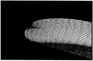
Fig. 15 Magnified view of grid at bow (a ship with a rudder).
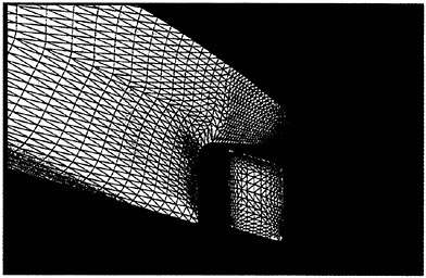
Fig. 16 Magnified view of grid at stern (a ship with a rudder).
Computed pressure distribution is shown in Figs. 17, 18 and 19. Contour lines occasionally show unnatural kink. This is supposed to be a plotting problem. The high pressure region can be seen in the leading edge of the rudder in Fig. 19. The pressure distribution on a ship hull in Fig. 19 is not so different from that of Fig. 10, that shows a hull surface pressure is insensitive to the presence of a rudder.
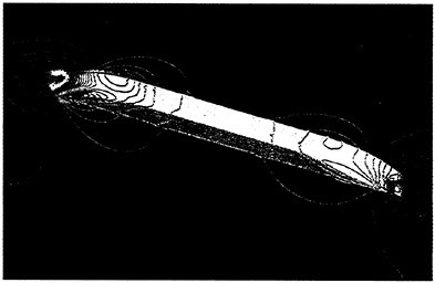
Fig. 17 Computed pressure distribution (a ship with a rudder).
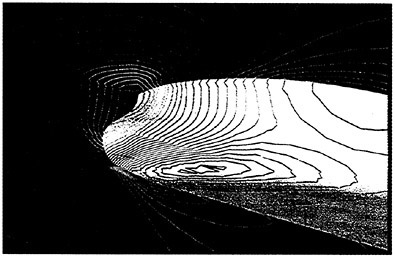
Fig. 18 Computed pressure distribution at bow (a ship with a rudder).
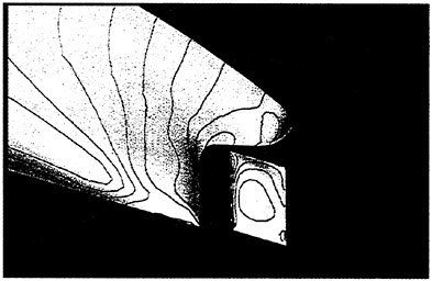
Fig. 19 Computed pressure distribution at stern (a ship with a rudder).
Fig. 20 shows the comparison of the hull surface pressure distribution of computation and the experiment (22). Good agreement can be seen between the two pressure patterns. The extent of the low
pressure zone at the bilge and the high pressure region at the edge of stern overhang are well simulated by the present solver.
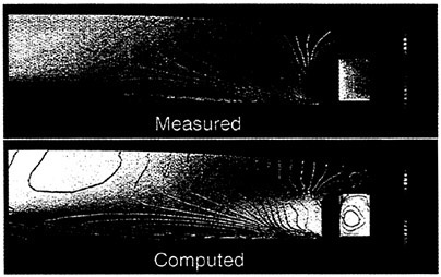
Fig. 20 Comparison of measured (top) and computed (bottom) pressure distributions on a ship hull.
Figs. 21 and 22 show the velocity distribution on the propeller plane and on the aft perpendicular section. The wake distribution on the propeller plane does not show the so-called ‘hook’ shape clearly. The pattern is rather similar to the one with the Spalart-Allmaras models shown in Fig. 13. The difference between Figs. 21 and 12 seems to be due to the grid topology. In the O-O topology shown in Fig. 6, the grid spacing just behind the hull is as small as the other cells next to a hull. On the other hand, in the H-O topology shown in Fig. 16, the grid spacing behind the hull is a few orders magnitude larger than the usual minimum spacing in the wall normal direction. The boundary values of the ω on the wall are very large and ![]() since ω is responsible for a near wall damping of the eddy viscosity. The free stream value of ω, on the other hand is
since ω is responsible for a near wall damping of the eddy viscosity. The free stream value of ω, on the other hand is ![]() . Therefore, ω must decreases rapidly inside the boundary layer. The large grid spacing behind a hull with the H-O topology (Fig. 16) may not be fine enough to resolve the steep gradient of ω in this region. Further investigations are needed to clarify this issue.
. Therefore, ω must decreases rapidly inside the boundary layer. The large grid spacing behind a hull with the H-O topology (Fig. 16) may not be fine enough to resolve the steep gradient of ω in this region. Further investigations are needed to clarify this issue.
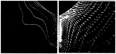
Fig. 21 Computed velocity distributions at propeller plane. Axial velocity contours and crossflow vectors
In Fig. 22, the wake is divided by the rudder. At the leading and the trailing edges of the rudder, the grid spacing is again very large and the same problem as above may arise. By using a truly unstructured grid with the control of the minimum spacing on the wall, these problems can be avoided.
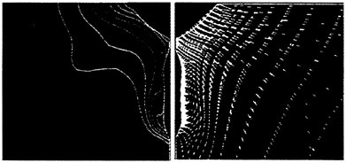
Fig. 22 Computed velocity distributions at AP section. Axial velocity contours and crossflow vectors
4 Concluding Remarks
An unstructured grid method has been developed for simulating three-dimensional incompressible viscous flows around a complex configuration. The numerical method solves the Navier-Stokes equations with artificial compressibility using a finite volume method on an unstructured grid. Time integration is carried out by the backward Euler method. The derived linear system is solved by the Gauss-Seidel iteration. The k-ω-SST two equation turbulence model is used for high Reynolds flow simulations.
Three dimensional computations are carried out for a tanker hull and a tanker with a rudder configuration. Both results show reasonable agreements with the experimental data and the applicability of the present solver has been proved. The k-ω-SST turbulence model shows promising performance with respect to the prediction of the wake pattern when used with the appropriate grid.
Future plans include the application to truly unstructured grid cases and the extension to free surface flows.
Acknowledgment
The author would like to thank Dr. M.Hinatsu of Ship Research Institute for providing the structured grid and the informations of the experiments for a ship hull with a rudder configuration. Also, discussions and suggestions from members of the CFD group at Ship Research Institute are gratefully acknowledged.
REFERENCES
1. Mavriplis, D.J., “Unstructured Grid Techniques”, Annual Review on Fluid Mechanics, Vol. 29, 1997, pp. 473–514.
2. Venkatakrishnan, V., “A Perspective on Unstructured Grid Flow Solvers”, AIAA Journal, Vol. 34, No. 3, March 1996, pp. 533–547.
3. Jameson, A. Baker, T.J. and Weatherill, N.P., “Calculation of Inviscid Transonic Flow Over a Complete Aircraft”, AIAA Paper 86–0103, 1986, American Institute of Aeronautics and Astronautics.
4. Chen A. and Kallinders Y., “Adaptive Hybrid (Prismatic/Tetrahedral) Grids for 3-D Incompressible Flows”, AIAA Paper 96–0293, 1996, American Institute of Aeronautics and Astronautics.
5. Anderson, W.K., Rausch, R.D. and Bonhaus, D.L., “Implicit/Multigrid Algorithms for Incompressible Turbulent Flows on Unstructured Grids”, Journal of Computational Physics, Vol. 128, 1996, pp. 391–408.
6. Hino, T., Maritinell, L. and Jameson, A., “A Finite-Volume Method with Unstructured Grid for Free Surface Flow Simulations”, Proceedings of the Sixth International Symposium on Numerical Ship Hydrodynamics, Iowa City, 1993, pp. 173–193.
7. Hino, T., “An Unstructured Grid Method for Incompressible Viscous Flows with a Free Surface”, AIAA Paper 97–0862, 1997, American Institute of Aeronautics and Astronautics.
8. Lohner, R., Yang, C., Oñate, E. and Idelssohn, A., “An Unstructured Grid-Based, Parallel Free Surface Solver”, AIAA Paper 97–1830, 1997, American Institute of Aeronautics and Astronautics.
9. Hino T, “A 3D Unstructured Grid Method for Incompressible Viscous Flows”, Journal of the Society of Naval Architects of Japan, Vol. 182, 1997, pp. 9–15.
10. Roe, P.L., “Characteristic-Based Schemes for the Euler Equations”, Annual Review on Fluid Mechanics, Vol. 18, 1986, pp. 337–365, (1986).
11. Barth, T.J., “A 3-D Upwind Euler Solver for Unstructured Meshes”, AIAA Paper 91–1548-CP, 1991, American Institute of Aeronautics and Astronautics.
12. Barth, T.J. and Jespersen D.C., “The Design and Application of Upwind Schemes on Unstructured Meshes”, AIAA Paper 89–0366, 1989, American Institute of Aeronautics and Astronautics.
13. Rausch, R.D., Batina J.T. and Yang H.T.Y., “Spatial Adaption Procedures on Unstructured Meshes for Accurate Unsteady Aerodynamic Flow Computation”, ΑΙAA Paper 91–1106, 1991, American Institute of Aeronautics and Astronautics.
14. Spalart, P.R. and Allmaras S.R., “A One-Equation Turbulence Model for Aerodynamic Flows”, La Recherche Aérospatiale, No. 1, 1994, pp. 5–21.
15. Menter, F.R., “Two-Equation Eddy-Viscosity Turbulence Models for Engineering Application”, AIAA Journal, Vol. 32, No. 8, August 1994, pp. 1598–1605.
16. Wilcox, D.C., “Reassessment of the Scale-Determining Equation for Advanced Turbulence Models”, AIAA Journal, Vol. 26, No. 11, November 1988, pp. 1299–1310.
17. Deng, G. and Visonneau, M., “Evaluation of Eddy Viscosity and Second-Moment Turbulence Closures for Steady Flows Around Ships”, Proceedings of the Twenty-First Symposium on Naval Hydrodynamics, 1997, pp. 453–467.
18. Suzuki, T., Okuni, T., Nozawa, K. and Suzuki, H., “Characteristics of Turbulent Boundary Layer in a Stern Flow Field with Longitudinal Vortices”, Proceedings of the Twenty-Seventh Symposium on Turbulence, 1995, pp. 133–136 (in Japanese).
19. Hino, T., “Viscous Flow Computations around a Ship Using One-Equation Turbulence Models”, Journal of the Society of Naval Architects of Japan, Vol. 178, 1995, pp. 9–22.
20. Ogiwara, S., “Stern Flow Measurements for The Tanker ‘Ryuko-Maru’ in Model Scale, Intermediate Scale and Full Scale Ships”, Proceedings of CFD Workshop Tokyo 1994, Vol. 1, 1994, pp. 341–349.
21. Hinatsu, M., Hino, T., Kodama, Y., Fujisawa, J. and Ando J., “Numerical Simulation of Flow around Ship Hull with Rudder in Self Propulsion Condition”, Transaction of the West Japan Society of Naval Architects, No. 90, 1995, pp. 1–10 (in Japanese).
22. Hinatsu, M., Takeshi, H., Fujisawa, J. and Tsukada, Y., “Pressure Measurement around Full Ship Stern in Self Propulsion Condition”, Proceedings of the Sixty-Fourth General Meeting of Ship Research Institute, 1994, pp. 205–206 (in Japanese).
DISCUSSION
K.Mori
Hiroshima University, Japan
Is your point that the grid arrangement is more important than the turbulent model to realize the “hook-shaped” wake contour?
AUTHOR’S REPLY
It is the turbulence modeling that is responsible for reproduction of the wake distribution. Some turbulence models require the grid property suitable for the models in order to work as designed. In the case of the present paper, the k-w-SST model appears to work well only when used with a grid of O-O type topology, although further verification is needed. In summary, to simulate flow fields accurately, one needs (1) an appropriate turbulence model, (2) a grid which is suitable for the turbulence model used and, of course, (3) a reliable flow solver.
Viscous Free Surface Hydrodynamics Using Unstructured Grids
R.Löhner, C.Yang (George Mason University, USA)
E.Oñate (Universidad Politécnica de Catalunya, Spain)
ABSTRACT
An unstructured grid-based, parallel solver has been developed for solving viscous free surface hydrodynamics problems. The overall scheme combines a finite-element, equal-order, projection-type three-dimensional incompressible flow solver with a finite element, two-dimensional advection equation solver for the free surface equation. The solution is marched in time until a steady state is reached. The unstructured grid enhances geometrical flexibility when treating complex geometries, and the parallel implementation permits fast turnaround of numerical simulations. A number of flows of practical interest are analyzed to demonstrate the numerical performance of the present approach.
1. INTRODUCTION
The prediction of the Kelvin wave pattern and wave resistance of ships has challenged mathematicians, hydrodynamicists and naval architects for over a century. Only in recent years has the rapid development of computer hardware and software enabled large-scale computer simulation of steady ship waves.
The Boundary Element Method is a widely used approach for the prediction of the ideal wave pattern of ships advancing with constant forward speed. There exist two main types of elementary singularity in the solution schemes of this method. The first class of schemes uses the Kelvin wave source as the elementary singularity. The major advantages of such a scheme are the elimination of the integration over the free surface from the resulting boundary integral equation and the automatic satisfaction of the radiation condition. However, this scheme cannot be extended to include nonlinear wave effects. The theoretical background of this method was reviewed by Wehausen (1970), while computational aspects can be found in the literature and in a series of Ship Wave Resistance Workshops (Workshop on Ship Wave Resistance Computations, 1979, 1983). Noblesse et al. (1996) recently developed a new theoretical formulation, called Fourier-Kochin theory, which offers an alternative way of solving steady wave problems using this class of elementary source. The second class of schemes uses the Rankine source as the elementary source. This scheme was first presented by Dawson (1977). The Dawson method has been applied widely as a practical method for predicting wave resistance, and many improvements have been made to account for the nonlinear effects. Among them a successful example is the Rankine Panel Method (Dawson, 1977; Xia, 1986; Jenson and Soding, 1989; Kim and Lucas, 1990; Reed et. al., 1990; Nakos and Sclavounos, 1990; Raven, 1992; Beck et. al., 1993; Soding, 1996; Raven, 1996; Janson and Larsson, 1996). Considerable effort has been devoted to increasing efficiency and accuracy, resulting in the so-called patch method, desingularized method, RAPID method and etc. From the point of view of ship design, the Rankine Panel Method still has an unacceptable sensitivity to numerical parameters such as the domain size and paneling.
In recent years, the advent of advanced numerical schemes for the Euler and Navier-Stokes equations has enabled a more realistic prediction of wave resistance. In these schemes, a three-dimensional, i.e. volumetric incompressible flow solver is coupled with a free surface equation. The velocities obtained at the free surface from the three-dimensional incompressible flow solver are given to the free surface solver to update the free surface height. This new height changes the (prescribed) pressure at the free surface for the three-dimensional incompressible flow solver, closing the loop. The free surface height also serves as the basis for the mesh motion.
There exist two main types of incompressible flow solvers. The first class is based on projection schemes (Chorin, 1968; Kim and Moin, 1985; Hino, 1989; Martin and Löhner, 1992; Luo et. al., 1995; Alessandrini and Delhommeau, 1996; Miyata, 1996; Kallinderis and Chen, 1996; Ramamurti and Löhner, 1996; Löhner et. al., 1997). A velocity field is predicted in a first step. The conservation of mass is enforced in a second step by solving a Poisson equa-
tion, which results in a new pressure. Finally, the velocity field is updated with this new pressure.
The second class is based on artificial compressibility schemes (Chorin, 1967; Rizzi and Eriksson, 1985; Hino et. al., 1993; Farmer et. al., 1994; Peraire et. al., 1994; Martinelli and Farmer, 1994; Cowles and Martinelli, 1996; Hino, 1997). The infinite speed of sound of the incompressible medium is reduced to a finite number by adding a time derivative of the pressure to the divergence equation. This enables the effective use of all the techniques developed for compressible flow simulation, such as limitors, upwind differencing, residual smoothing, multigrid acceleration, etc. At steady state, the time derivative in the divergence equation vanishes, yielding the proper incompressible solution.
Both families of solvers have been used successfully for free surface prediction. The projection scheme is adopted in the present study, because the pressure is specified over a considerable portion of the domain (free surface, entry plane, and bottom), resulting in very fast convergence for the Poisson solver.
According to Moore’s law, computer memory and speed increase by a factor of 10 every 5 years. This implies that sooner or later the human cost of setting up problems will be the only barrier to widespread use of numerical predictions. The only way to eliminate the cost of set-up times is via fully automatic grid generators which are linked directly to a CAD database. To date, the only automatic grid generators are those for unstructured grids, be they either of tetrahedral or Cartesian (Welterlen, 1995; Aftosmis, 1997) space discretizations. Given the difficulty of Cartesian grids to generate proper discretizations for RANS calculations, we opted for tetrahedra.
The present paper is organized as follows: Section 2 summarizes the equations used to describe the flow and free surface; Section 3 describes the numerical methods used to solve these equations; Sections 4–6 are devoted to unstructured grid generation, mesh update and parallelization; some examples are shown in Section 7; finally, some conclusions are drawn and an outlook for further research is given in Section 8.
2. MATHEMATICAL FORMULATION
Figure 1 shows the reference frame and ship location used in this paper. A Cartesian coordinate system Oxyz is fixed to the ship with the origin inside the hull on the mean free surface. The z direction is positive upwards, y is positive towards the starboard side and x is positive in the aft direction. The free stream velocity vector is parallel to the x axis and points in the same direction.
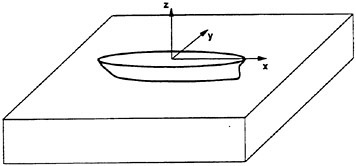
Figure 1 Coordinate System Used
2.1 Flowfield Equations
The equations solved are the incompressible Reynolds-Averaged Navier-Stokes equations, given, in non-dimensional form, by the conservation of mass and momentum:
(1)
(2)
where v=(u, v, w) denotes the velocity vector and Ψ the pressure plus hydrostatic pressure:
(3)
and Re the Reynolds-number Re=V∞L/ν∞. A particle on the free surface must remain so for all times, which implies that the free surface elevation β obeys the advection equation
(4)
The boundary conditions are as follows:
-
Inflow Plane: At the inflow plane, the velocity, pressure and free surface height are prescribed:

(5)
-
Exit Plane: At the exit plane, none of the quantities are prescribed. The natural Neumann conditions for the pressure and extrapolation boundary conditions for the velocities and free surface height are imposed automatically by the numerical scheme used.
-
Free Surface: At the free surface, the pressure p is prescribed to be p=0, implying that Ψ is given by
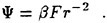
(6)
-
The velocity is allowed to float freely, allowing leakage of fluid through the free surface.
-
Bottom: At the bottom, one may either impose the boundary conditions for a
-
Wall: vanishing normal velocity, Neumann conditions for the pressure, or
-
Infinite Depth: prescribed pressure, no boundary conditions for the velocities.
-
-
Ship Hull: Depending on the turbulence model used, the velocity (laminar, Baldwin-Lomax, low-Re k−∈) or only its normal component (Euler, high-Re k−∈) must vanish, i.e.
(7a, b)
where n is the normal to the hull.
-
Side Walls: On the side walls of the computational domain, we impose vanishing normal velocity.
2.2 Turbulence Modeling
The effects of turbulence are modeled by either using the Baldwin-Lomax or the k−∈ model.
2.2.1 Baldwin-Lomax Model
The Baldwin-Lomax model (Baldwin, 1978) assumes that the flow consists of an inner and an outer part, where:
a) Inner part: y<yc
(8a)
b) Outer part: y>yc
(8b)
(8c)
(8d)
The term ![]() is the so-called van Driest damping factor. This model represents one of the simplest and most accurate ones available wherever applicable. Being of algebraic nature, it is very fast, and adds a slight CPU-penalty as compared to laminar flow simulations. It requires special data structures and the associated storage for the wall normals, and does not perform well for separated flows. A drawback of the model is that for wakes, no reliable extensions exist. Furthermore, action must be taken in the wake and in order not to obtain Ymax values that are too large, and hence turbulence viscosities that are unrealistic.
is the so-called van Driest damping factor. This model represents one of the simplest and most accurate ones available wherever applicable. Being of algebraic nature, it is very fast, and adds a slight CPU-penalty as compared to laminar flow simulations. It requires special data structures and the associated storage for the wall normals, and does not perform well for separated flows. A drawback of the model is that for wakes, no reliable extensions exist. Furthermore, action must be taken in the wake and in order not to obtain Ymax values that are too large, and hence turbulence viscosities that are unrealistic.
2.2.2 k−∈-Model
This two-equation model has been extensively used, and has become a standard model for many flow codes. Denoting by k the turbulent kinetic energy and ∈ the dissipation rate, the field equations are given by:
(9a)
(9b)
(9c)
with the common constants:
cμ=0.09, c1=1.44, c2=1.92, c3=0.80 σk=1.00, σ∈=1.30, σT=0.90.
If a full discretization to the wall is attempted, the boundary conditions are given by v=0, k=0. In case we use the ‘law of the wall’ approximation, we have v · n=0, a shear stress τω
(10)
and ![]() .
.
3. NUMERICAL IMPLEMENTATION
For the solution of the 3-D incompressible flow equations, a pressure projection scheme is used. In this way, the pressures are integrated implicitly, correctly reflecting the infinite propagation speed of sound. A complete timestep consists of three parts:
a) Advective-Diffusive Prediction: vn→v*
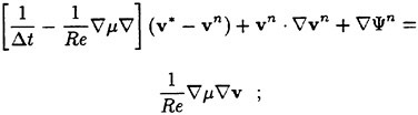
(11)
b) Pressure Correction: Ψn→Ψn+1
(12a)
(12b)
which results in
(13)
c) Velocity Correction: v*→vn+1
(14)
Observe that at steady state, the residuals of the pressure correction vanish, implying that the result is neither dependent on the projection scheme itself nor the timestep Δt.
3.1 Spatial Discretization
The spatial discretization of the first-order derivatives via the Galerkin weighted residual method using linear elements results in an edge-based loop for the right-hand sides of the form:
(15)
where ![]() contains all the geometric parameters associated with the elements surrounding the edge i, j and the dimension k. The inner product over the dimensions k may be written in compact form as
contains all the geometric parameters associated with the elements surrounding the edge i, j and the dimension k. The inner product over the dimensions k may be written in compact form as
(16)
where the fi are the ‘fluxes along edges’, obtained from the scalar product
(17)
For the advective terms we have:
(18)
where
(19)
This form of the fluxes is of central difference character, and must be replaced by a consistent or stabilized numerical flux. For the advection system given by Eqn. (4), this results in
(20)
where
(21)
This first-order scheme is improved to second order by replacing the values of vi, vj by improved or reconstructed values vi′, vj′. Standard MUSCL limiting procedures [Le74] are used to obtain monotonicity preserving solutions even in the pure advection (i.e. Euler) case.
For the continuity equation, the edge-based expression used is:
(22)
where
(23)
A consistent or stabilized numerical flux is given by:
(24)
with
(25)
Here Δt and l are a characteristic advective timestep and length of the edge. This first-order scheme is replaced by a higher-order scheme of the form
(26)
which is reminiscent of a fourth-order damping term for the divergence equation (Peraire et. al., 1994, Kallinderis and Chen, 1996).
The spatial discretization of the second-order derivatives via the Galerkin weighted residual method using linear elements results in an edge-based loop for the right-hand sides of the form:
(27)
where ![]() contains all the geometric parameters associated with the elements surrounding the edge i, j for the Laplacian operator.
contains all the geometric parameters associated with the elements surrounding the edge i, j for the Laplacian operator.
3.2 Free Surface Discretization
The free surface equation (4) is treated as a standard scalar advection equation with source terms for the x, y plane. The faces on the free surface are extracted from the three-dimensional volume grid. Points and elements are renumbered locally to obtain a two-dimensional triangular finite element mesh in x, y. As before, the spatial discretization of the advective fluxes results in
(28)
Fourth-order damping is added to stabilize these central difference terms, resulting in
(29)
Following Hino et. al. (1993), an additional damping term is added to the free surface equation near inflow and outflow boundaries, resulting in
(30)
where dh(x), for the outflow boundary, is given by
(31)
and c1 is a parameter of O(1). A similar expression is applied at the inflow boundary for steady-state problems. The vertical velocity w, as well as the additional damping term, are evaluated by simply using the lumped mass matrix. In order to damp out the wave height β completely at the downstream boundary, the w-velocity obtained from the three-dimensional incompressible flow solver is modified, yielding
(32)
where dw(x) is given by the Hermitian polynomial
(33)
and ξ is defined in Eqn. (31). The final semi-discrete scheme takes the form:
(34)
where the subscripts a, s, d stand for advection, source and damping. This system of ODE’s is integrated in time using a standard five-stage Runge-Kutta scheme.
3.3 Overall Scheme
One complete timestep consists of the following steps:
-
Given the boundary conditions for the pressure Ψ, update the solution in the three-dimensional fluid mesh (velocities, pressures, turbulence variables);
-
Extract the velocity vector v=(u, v, w) at the free surface and transfer it to the two-dimensional free surface module;
-
Given the velocity field, update the free surface β;
-
Transfer back the new free surface β to the three-dimensional fluid mesh, and impose new boundary conditions for the pressure Ψ.
For steady-state applications, the fluid and free surface domains are updated using local timesteps. This allows some room for variants that may converge faster to the final solution, e.g. n steps of the fluid followed by m steps of the free surface, complete convergence of the free surface between fluid updates, etc. We have experimented with some of these. The results show that most of these variants prove unstable, or do not accelerate convergence measurably. Our current preference for steady-state applications is to use an equivalent ‘time-interval’ ratio between fluid and free surface of 1:8, e.g. a Courant-nr. of Cf=0.25 for the fluid and Cs=2.0 for the free surface.
4. UNSTRUCTURED GRID GENERATION
Viscous runs are not only more difficult than inviscid ones because of the increased complexity of physical models. Most of the practical difficulties stem from the fact that the generation of proper grids is more involved. Optimal grids for RANS calculations are characterized by narrow regions with extreme grid distortion, mimicking the location and movement of boundary and shear layers.
Most isotropic mesh generation techniques tend to fail when attempting to generate highly stretched elements, a key requirement for Reynolds-Averaged Navier Stokes (RANS) calculations with turbulence models that reach into the sublayer. A number of specialized schemes have been proposed to remedy this situation (Nakahashi, 1987; Kallinderis, 1992; Löhner, 1993; Pirzadeh, 1994; Marcum, 1995; Pirzadeh, 1996; Peraire and Morgan, 1996). The domain to be gridded was divided into isotropic and stretched element regions. In addition, a blending procedure to transition smoothly between these zones was provided. Typically, the stretched mesh region was generated first (Kallinderis, 1992; Löhner, 1993; Pirzadeh, 1994; Marcum, 1995; Pirzadeh, 1996). Although we have used such a scheme (Löhner, 1993) for a number of years, we have found several situations in which the requirement of a semi-structured element or point placement close to wetted surfaces is impossible, prompting us to search for a more general technique.
The path taken here may be summarized as follows:
-
Generate an isotropic mesh; this can be done with any unstructured grid generator;
-
Using a constrained Delaunay technique, introduce points in order to generate highly stretched elements;
-
Introduce the points in ascending level of stretching, i.e. from the domain interior to the boundary.
This procedure has the following advantages:
-
No surface recovery is required for the Delaunay reconnection, eliminating the most problematic part of this technique;
-
The meshing of concave ridges/corners requires no extra work;
-
Meshing problems due to surface curvature are minimized;
-
In principle, no CAD representation of the surface is required; and
-
It guarantees a final mesh, an essential requirement for automation.
The disadvantages are the following:
-
As with any Delaunay technique, the mesh quality is extremely sensitive to point placement.
The discretization of a general three-dimensional computational domain into an unstructured assembly of isotropic tetrahedra is accomplished by means of an advancing front grid generation procedure (Löhner, 1997). This requires that the geometry of the computational domain be defined first in terms of an assembly of surface patches, and the spatial variation of element size and shape be prescribed in a number of ways. The first step in the process is the triangulation of the computational boundary surfaces. The assembly of resulting triangles forms the initial front for the three-dimensional grid generation process. The advancing front method is then used to fill the computational domain with tetrahedra, which are generated so as to meet a user-prescribed distribution of element size and shape. Both analytical surface patches (planes, Coon’s patches etc.) and discrete surface patches (defined by a surface triangulation) are used to define the boundaries of the computational domain. The hull offset data is triangulated directly. This triangulation is subsequently used to define, in a discrete manner, the hull surface. The rest of the boundary surfaces are defined analytically.
5. MESH UPDATE STRATEGY
Previous work by Hino (1993; 1997) and Farmer et al. (1994) marched the solution in time until a steady-state was reached. At each timestep, a volume update was followed by a free surface update. The repositioning of points at each timestep implies a complete recalculation of geometrical parameters, as well as interrogation of the CAD information defining the surface. In our case, this would double CPU requirements. For this reason, when solving steady-state problems, we do not move the grid at each timestep, but only change the pressure boundary condition after each update of the free surface β. The mesh is updated every 100–250 timesteps, thereby minimizing the costs associated with geometry recalculations and grid repositioning along surfaces. We have observed that this strategy has the advantage of not moving the mesh unduly at the beginning of a run, where large wave amplitudes may be present. One mesh update consists of the following steps:
-
Obtain the new elevation for the points on the free surface from β. This only results in a vertical (z-direction) displacement field dΓ for the boundary points.
-
Apply the proper boundary conditions for the points on the waterline. This results in an additional horizontal (x,y-direction) displacement field for the points on the water line.
-
Smooth the displacement field in order to avoid mesh distortion. The smoother used is of the form (Löhner and Yang, 1996):
(35)
where k is a nonlinear stiffness coefficient that depends on the distance from the hull.
-
Interrogate the CAD data to reposition the points on the hull.
Denoting by d*, n, t the predicted displacement of each point, surface normals and tangential directions, the boundary conditions for the mesh movement are as follows (see Figure 2):
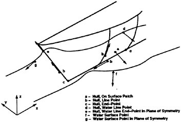
Figure 2 Boundary Conditions for Mesh Movement
-
Hull, On Surface Patch: The movement of these points has to be along the surface, i.e. the normal component of d* is removed:
(36)
-
Hull, Line Point: The movement of these points has to be along the lines, resulting in a tangential boundary displacement of the form:
(37)
-
Hull, End-Point: No displacement is allowed for these points, i.e. d=0;
-
Hull/Water Line Point, Water Line End-Point: The displacement of these points is fixed, given
-
by the change in elevation Δz and the surface normal of the hull. Defining d0=(0, 0, Δz), we have
(38)
-
Hull/Water Line End-Point in Plane of Symmetry: The displacement of these points is fixed, and dictated by the tangential vector to the hull-line in the symmetry plane:
(39)
-
Water Surface Points: These points start with an initial displacement do, but may glide along the water surface, allowing the mesh to accommodate the displacements in the x,y-directions due to points on the hull. The normal to the water line is taken, and Eqn. (36) is used to correct any further displacements.
-
Water Surface Points in Plane of Symmetry: As before, these points start with an initial displacement d0, but may glide along the water surface, remaining in the plane of symmetry, thus allowing the mesh to accommodate the displacements in the x-direction due to points on the hull. The tangential direction is obtained from the sides lying on the water surface in the plane of symmetry, and Eqn. (37) is used to correct any further displacements.
An option to restrict the movement of points completely in certain regions of the mesh has been found useful. Regions where such an option is required are transom sterns, as well as the points lying in the half-plane given by the minimum z-value of the hull. Should negative elements arise due to surface point repositioning, they are removed and a local remeshing takes place. Naturally, these situations should be avoided as much as possible.
6. PARALLELIZATION
In order to integrate the numerical simulation techniques into ship design practice, the numerical solution process predicting nonlinear ship waves must be both accurate and efficient. Given that most advanced computer architectures achieve speed by some form of parallelism, the present solution algorithms were modified for efficient parallelization. For distributed memory machines, parallelization is accomplished via domain decomposition with message passing at interface boundaries (Löhner and Ramamurti, 1995; Ramamurti and Löhner 1996). For shared-memory, cache-based machines with multiple CPUs, such as SGI Origin 2000, a renumbering and regrouping technique for points and edges is developed to achieve good parallel performance, i.e., to perform well on each processor and allow pipelining. Cache-misses are reduced by renumbering the points, so that any required point information for edges is as close as possible in memory when required by an edge. The edges are renumbered in such a way that, as the loop progresses through the edges, the point information should be accessed as uniformly as possible (Löhner, 1993). Memory contention issues are avoided by regrouping edges such that none of the points are accessed by the edges in each group more than once. Furthermore, the edges are renumbered to achieve pipelining and parallelization by processing all the individual vector-groups in parallel at a high level, in such a way that the point-range between macro-groups does not overlap (Löhner, 1997).
Table 1 shows the speed-up observed on a loaded 16-processor R10000 SGI Origin 2000 for 100 timesteps. The times quoted are for a RANS run using the k−∈ model, a mesh of approximately 1 Mtet, include solvers, input/output, movie dump-files, build up of data structures, etc., and may therefore be considered realistic.
Table 1: Timings for Wigley Hull (R-10000)
|
nproc |
time (sec) |
CPU (sec) |
Speedup |
|
1 |
3044 |
3001 |
1.00 |
|
2 |
1837 |
3537 |
1.65 |
|
4 |
1175 |
4362 |
2.59 |
|
6 |
1043 |
5683 |
2.91 |
7. NUMERICAL RESULTS
The solution algorithm outlined in the preceeding sections has been applied to the prediction of steady wave patterns for a number of hull forms over a wide range of Froude numbers. For all of these cases, local timestepping was employed for the three-dimensional incompressible flow solvers as well as the free surface solver. At the start of a run, the three-dimensional flowfield was updated for 10 timesteps without any free surface update. Thereafter, the free surface was updated after every three-dimensional flowfield timestep. The mesh was moved every 100–250 timesteps. All simulations were run on a 16-processor R-10000 SGI Origin 2000 in shared-memory mode.
7.1 Submerged NACA0012
The first case considered is a submerged NACA0012 at α=5° angle of attack. This same configuration was tested experimentally by Duncan (1983) and modelled numerically by Hino (1993; 1997). Although
the case is two-dimensional, it was modelled as three-dimensional, with two parallel walls in the y-direction. The mesh consisted of 2,409,720 tetrahedral elements, 465,752 points and 115,093 boundary points, of which 6,929 were on the free surface. The Froude number was set to Fr=0.5672. This case was run in Euler mode and using the Baldwin-Lomax model with a Reynolds-nr. of Re=106. Figures 3a–f show, respectively, the surface grid, pressure and velocity fields, as well as a zoom of the velocity field close to the airfoil. Note the boundary layer from the velocity fields. Figure 3g compares the wave profiles for the Euler, Baldwin-Lomax, Hino’s (1993) Euler and Duncan’s (1983) experiment data. The wave amplitudes are noticeably lower for the RANS case. This was also observed by Hino (1997).
7.2 Wigley Hull
The second case considered is the well known Wigley Hull, given by the analytical formula:
(40)
where Β and D are the beam and the draft of the ship at still water. For the case considered here, we had D=0.0625 and B=0.1. This same configuration was tested experimentally at the University of Tokyo (1983) and modelled numerically by Farmer (1994), Raven (1996) and others. We first generated a fine triangulation for the surface given by Eqn. (40). This triangulation was subsequently used to define, in a discrete manner, the hull. The surface definition of the complete computational domain consisted of discrete (hull) and analytical surface patches. The mesh consisted of 1,119,703 tetrahedral elements, 204,155 points and 30,358 boundary points, of which 15,515 were on the free surface. The parameters for this simulations wre as follows: Fr=0.25, Re=106, and k−∈ model with law of the wall approximation. Figures 4a,b show the surface grids employed, and the extent of the region with high aspect ratio elements. In Figures 4c,d the wave profiles and surface velocities obtained from Euler and RANS calculations are comprared. As expected, the effect of viscosity becomes noticeable in the stern region. Figure 4e shows the comparison to the experiments conducted at the University of Tokyo. It can be noticed that the first wave is accurately reproduced, but that the second wave is not well reproduced by the calculations. We are currently reviewing possible causes for this mismatch (hull definition, trimm, experimental errors, etc.).
7.3 Double Wigley Hull
The third case considered is an inviscid case comprising two Wigley hulls positioned close to each other. and is intended to show the flexibility of the proposed method for situations with rapid change in design. A number of cases were run in a matter of days, of which the most relevant are summarized here. Figures 5a–f show the resulting wave pattern for a Froude-nr. of Fr=0.316 for different relative spacings in the x-and y-directions. As one can see, the effect on the resulting wave pattern is considerable.
7.4 Wigley Carrier Group
The fourth case considered is again inviscid. The viscous simulation of this type of flow is being carried out at present. The configuration consists of a Wigley hull in the center that has been enlarged by a factor of 1:3, surrounded by normal Wigley hulls. The mesh consisted of approximately 4.2 Mtets. Figures 6a,b show the resulting wave patter for a Froude-nr. of Fr=0.316. CPU time for this problem was approximately 24 hours using 8 processors.
8. CONCLUSIONS AND OUTLOOK
An unstructured grid-based, parallel, viscous free surface solver has been developed. The overall scheme combines a finite-element, equal-order, projection-type three-dimensional incompressible flow solver with a finite element, two-dimensional advection equation solver for the free surface equation. For steady-state applications, the mesh is not moved every timestep in order to reduce the cost of geometry recalculations and surface repositioning. The results obtained show good quantitative comparison with experiments and the results of other techniques for different hull forms and a wide range of Froude numbers. The combination of unstructured grids (enhanced geometrical flexibility, fast problem set-up) and good parallel performance (rapid turnaround) should make the present approach attractive to hydrodynamic design simulations.
The present capability is considered only a first step in a much more ambitious undertaking. Future work will center on:
-
Extension to transient problems,
-
Acceleration techniques for steady-state,
-
Coupling to ship motion for seakeeping analysis,
-
Incorporation of further mesh movement options, and
-
Development of a toolkit for ship design practice.
9. ACKNOWLEDGEMENTS
This work was partially funded by AFOSR. Dr. Leonidas Sakell was the technical monitor. Additional funding was provided by NRL LCP&FD. Dr. William Sandberg was the technical monitor. The authors would also like to thank Dr. Francis Noblesse,
DTMB, for providing some of the data sets and experimental results, as well as his interest and encouragement.
10. REFERENCES
Aftosmis, M. and Melton, J. 1997 Robust and Efficient Cartesian Mesh Generation from Component-Based Geometry. AIAA-97–0196.
Alessandrini, B., Delhommeau, G. 1996 A Multigrid Velocity-Pressure- Free Surface Elevation Fully Coupled Solver for Calculation of Turbulent Incompressible Flow Around a Hull. Proceedings: Twenty-first Symposium on Naval Hydrodynamics. Trondheim, Norway, June.
Bai, K.J. and McCarthy J.H., Eds. 1979 Proceedings: Workshop on Ship Wave-Resistance Computations, Bethesda, MD, USA.
Baldwin, B.S. and Lomax, H. 1978 Thin Layer Approximation and Algebraic Model for Separated Turbulent Flows. AIAA-78–257.
Beck, R.F., Cao, Y., and Lee, T.-H 1993 Fully Nonlinear Water Wave Computations Using the Desingularized Method. Proceedings: Sixth International Conference on Numerical Ship Hydrodynamics. The University of Iowa, Iowa City, Aug.
Chorin, A.J. 1967 A Numerical Solution for Solving Incompressible Viscous Flow Problems. J. Comp. Phys. 2, 12–26.
Chorin, A.J. 1968 Numerical Solution of the Navier-Stokes Equations. Math. Comp. 22, 745–762.
Cowles, G. and Martinelli, L. 1996 Fully Nonlinear Hydrodynamic Calculations for Ship Design on Parallel Computing Platforms. Proceedings: Twenty-first Symposium on Naval Hydrodynamics. Trondheim, Norway, June.
Dawson, C.W. 1977 A Practical Computer Method for Solving Ship-Wave Problems. Proceedings: Second International Conference on Numerical Ship Hydrodynamics, USA.
Duncan, J.H. 1983 The Breaking and Non-Breaking Wave Resistance of a Two-Dimensional Hydrofoil. J. Fluid Mesh. 126, 507–516.
Farmer, J.R., Martinelli, L. and Jameson, A. 1993 A Fast Multigrid Method for Solving Incompressible Hydrodynamic Problems With Free Surfaces. AIAA J. bf 32, 6, 1175–1182.
Hino, T. 1989 Computation of Free Surface Flow Around an Advancing Ship by the Navier-Stokes Equations. Proceedings: Fifth International Conference on Numerical Ship Hydrodynamics. Hiroshima, Japan.
Hino, T., Martinelli, L. and Jameson, A. 1993 A Finite-Volume Method with Unstructured Grid for Free Surface Flow. Proceedings: Sixth International Conference on Numerical Ship Hydrodynamics. The University of Iowa, Iowa City, Aug.
Hino, T. 1997 An Unstructured Grid Method for Incompressible Viscous Flows with a Free Surface. AIAA-97–0862.
Janson, C. and Larsson, L. 1996 A Method for the Optimization of Ship Hulls from a Resistance Point of View. Proceedings: Twenty-first Symposium on Naval Hydrodynamics. Trondheim, Norway, June.
Jenson, G. and Soding, H. 1989 Ship Wave Resistance Computation. Finite Approximations in Fluid Mechanics, II 25.
Kallinderis, Y. and Chen, A. 1996 An Incompressible 3-D Navier-Stokes Method with Adaptive Hybrid Grids. AIAA-96–0293.
Kim, J. and Moin, P. 1985 Application of a Fractional-Step Method to Incompressible Navier-Stokes Equations. J. Comp. Phys. 59, 308–323.
Kim, Y.H. and Lucas, T. 1990 Nonlinear Ship Waves. Proceedings: Eighteenth Symposium on Naval Hydrodynamics. MI, USA.
ITTC 1983 Cooperative Experiments on Wigley Parabolic Models in Japan. 17th ITTC Resistance Committee Report, 2nd ed.
ITTC 1983 Cooperative Experiments on Series-60 Hull at UT-Tank. 17th ITTC Resistance Committee Report, 2nd ed.
Kallinderis, Y. and Ward, S. 1992 Prismatic Grid Generation with an Efficient Algebraic Method for Aircraft Configurations. AIAA-92–2721.
Löhner, R. 1993 Matching Semi-Structured and Unstructured Grids for Navier-Stokes Calculations. AIAA-93–3348-CP.
Löhner, R. 1993 Some Useful Renumbering Strategies for Unstructured Grids. Int. J. Num. Meth. Eng. 36, 3259–3270.
Löhner, R. and Ramamurti, R. 1995 A Load Balancing Algorithm for Unstructured Grids. Comp. Fluid Dyn. 5, 39–58.
Löhner, R. and Yang, C. 1996 Improved ALE Mesh Velocities for Moving Bodies. Comm. Num. Meth. Eng. 12, 599–608.
Löhner, R., Yang, C. and Baum, J.D. 1996 Rigid and Flexible Store Separation Simulations Using Adaptive Unstructured Grid Technologies. Proceedings: First AFOSR Conf. on Dynamic Motion CFD (L.Sakell and D.D.Knight eds.). Rutgers University, New Brunswick, New Jersey.
Löhner, R. 1997 Renumbering Strategies for Unstructured- Grid Solvers Operating on Shared-Memory, Cache-Based Parallel Machines. AIAA-97–2045-CP.
Löhner, R., Yang, C., Onate, E. and Idelssohn, S. 1997 An Unstructured Grid-Based, Parallel Free Surface Solver. AIAA-97–1830.
Löhner, R. 1997 Automatic Unstructured Grid Generators. Finite Elements in Analysis and Design 25, 111–134.
Luo, H., Baum, J.D. and Löhner, R. 1994 Edge-Based Finite Element Scheme for the Euler Equations. AIAA J. 32, 6, 1183–1190.
van Leer, B. 1974 Towards the Ultimate Conservative Scheme. II. Monotonicity and Conservation Combined in a Second Order Scheme. J. Comp. Phys. 14, 361–370.
Luo, H., Baum, J.D. and Löhner, R. 1995 A Finite Volume Scheme for Hydrodynamic Free Boundary Problems on Unstructured Grids. AIAA-95–0668.
Marcum, D.L. 1995 Generation of Unstructured Grids for Viscous Flow Applications. AIAA-95–0212.
Martin, D. and Löhner, R. 1992 An Implicit Linelet-Based Solver for Incompressible Flows. AIAA-92–0668.
Martinelli, L. and Farmer, J.R. 1994 Sailing Through the Nineties: Computational Fluid Dynamics for Ship Performance Analysis and Design. Chapter 27 in Frontiers of Computational Fluid Dynamics (D.A.Caughey and M.M.Hafez eds.), J.Wiley (1994).
Miyata, H. 1996 Time-Marching CFD Simulation for Moving Boundary Problems. Proceedings: Twenty-first Symposium on Naval Hydrodynamics. Trondheim, Norway, June.
Nakahashi, K. 1987 FDM-FEM Zonal Approach for Viscous Flow Computations over Multiple Bodies. AIAA-87–0604.
Nakos, D.E. and Sclavounos, P.D. 1990 On Steady and Unsteady Ship Wave Patterns. J. of Fluid Mechanics, 215, 256–288.
Noblesse, F. and McCarthy J.H., Eds. 1983 Proceedings: Second DTNSRDC Workshop on Ship Wave-Resistance Computations, Bethesda, U.S.A.
Noblesse, F., Chen, X.-B. and Yang, C. 1996 Fourier-Kochin Theory of Free Surface Flows. Proceedings: Twenty-first Symposium on Naval Hydrodynamics. Trondheim, Norway, June.
Peraire, J., Morgan, K. and Peiro, J. 1994 The Simulation of 3D Incompressible Flows Using Unstructured Grids. Chapter 16 in Frontiers of Computational Fluid Dynamics (D.A.Caughey and M.M.Hafez eds.), J.Wiley.
Peraire, J. and Morgan, K. 1996 Unstructured Mesh Generation Including Directional Refinement for Aerodynamic Flow Simulation. Proc. 5th Int. Conf. Num. Grid Generation in CFD and Related Fields, Mississippi, April.
Pirzadeh, S. 1994 Viscous Unstructured Three-Dimensional Grids by the Advancing-Layers Method. AIAA-94–0417.
Pirzadeh, S. 1996 Progress Towards a User-Oriented Unstructured Viscous Grid Generator. AIAA-96–0031.
Ramamurti, R. and Löhner, R. 1996 A Parallel Implicit Incompressible Flow Solver Using Unstructured Meshes. Computers and Fluids 5, 119–132.
Raven, H.C. 1992 A Practical Nonlinear Method for Calculating Ship Wavemaking and Wave Resistance. Proceedings: Ninteenth Symposium on Naval Hydrodynamics, Seoul, Korea.
Raven, H.C. 1996 A Solution Method for Nonlinear Ship Wave Resistance Problem. Doctoral Thesis, Maritime Research Institute, Netherlands.
Reed, A.M., Telste, J.G., Scragg, C.A. amd Liepmann, D. 1990 Analysis of Transom Stern Flows Proceedings: Seventeenth Symposium on Naval Hydrodynamics. The Hague, The Netherlands.
Rizzi, A. and Eriksson, L. 1985 Computation of Inviscid Incompressible Flow with Rotation. J. Fluid Mech. 153, 275–312.
Soding, H. 1996 Advances in Panel Methods. Proceedings: Twenty-first Symposium on Naval Hydrodynamics. Trondheim, Norway, June.
Wehausen, J.V. 1970 The Wave Resistance of Ships. Advances in Applied Mechanics.
Welterlen, T.J. and Karman, S.L. 1995 Rapid Assessment of F-16 Store Trajectories Using Unstructured CFD. AIAA-95–0354.
Xia, F. 1986 Numerical Calculation of Ship Flows with Special Emphasis on the Free Surface Potential Flow. Doctoral Thesis, Chalmers University of Technology, Sweden.
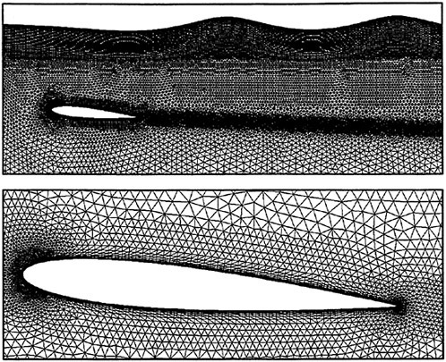
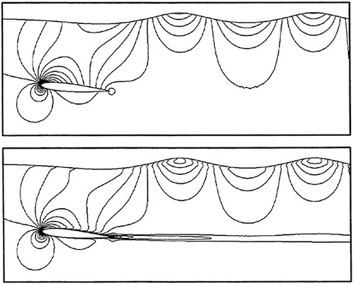
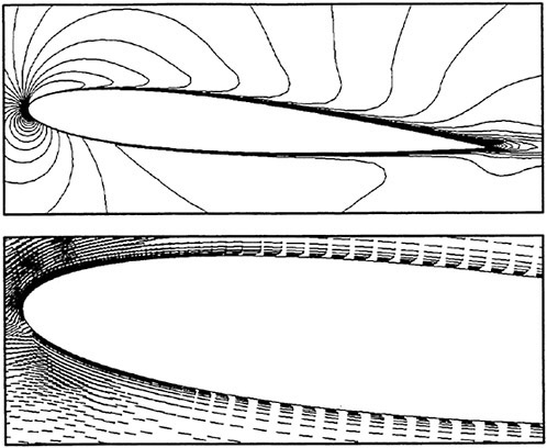
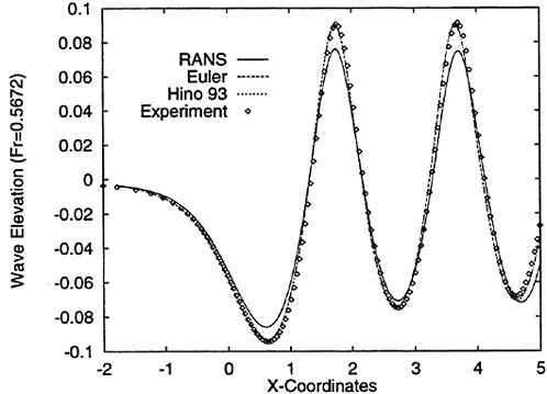
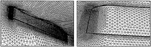
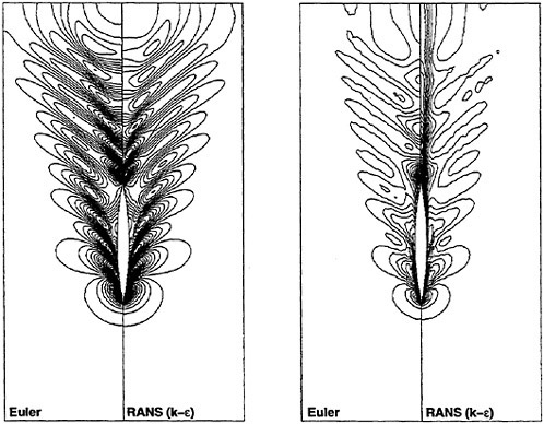
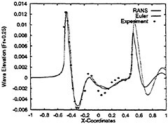
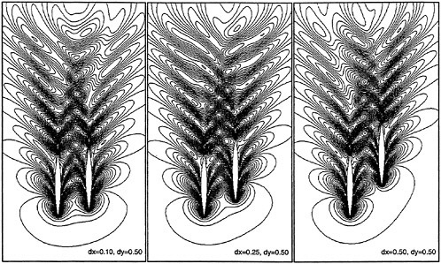
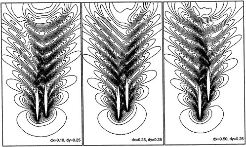
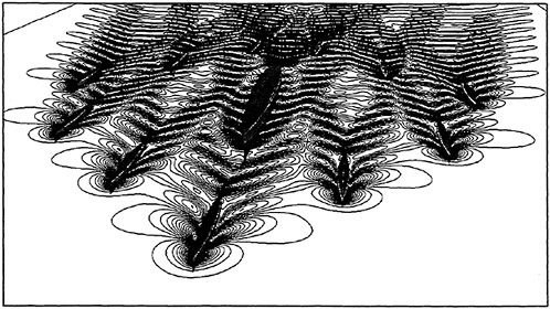

Viscous Free Surface Flow Past a Ship in Drift and in Rotating Motion
B.Alessandrini, G.Delhommeau (École Centrale de Nantes, France)
Abstract
This paper presents numerical simulations of three-dimensional unsteady viscous free surface flow past a ship in drift and in rotating motion using the Reynolds Averaged Navier-Stokes equations. An original fully coupled method for the velocities, pressure and free surface elevation discrete unknowns, already presented for symmetrical flows is used [1], [2]. The great challenge of this work is to generalize algorithms while preserving their efficiency in order to take into account non-symmetrical free surface flows. Numerical simulations are presented on the well known Series 60 CB=0.6 hull for two different cases: ship hull with attack angle and ship hull in forced giration.
1 Introduction
Numerical simulations of non-symmetrical ship flows remain a great challenge in the hydrodynamics community: current effects, drift effects on a sailing boat, or maneuvering effects, for examples, depend of the solution of this problem. The whole solution requires to compute three dimensional unsteady turbulent boundary layers with flow separation connected to complex free surface effects: Reynolds Averaged Navier-Stokes equations written under convective form in an unsteady curvilinear computational space fitted at each iteration to the hull and to the free surface are used. Fully non linear free surface conditions are solved using an efficient fully coupled algorithm [1], [2] and turbulence effects are taking into account through classical k−ω modelisation.
In fact, computation of non-symmetrical flows seems quite simple using a software suitable for symmetrical flows. The only one question is: how mass conservation and mean momentum conservation equations can be solved where topological boundaries do not coincide with physical boundaries, that is to say where physical boundary conditions cannot be applied. Classical way consists in using boundary overlapping and boundary conditions that traduce, implicitly or explicitly, the equality between boundary values and corresponding values in the internal domain. Using explicit boundary condition on topological boundaries is the most common option because of the easiness to implement it. Unfortunately this rudimentary method is not very efficient to solve velocity-pressure coupling, especially for unsteady flows, and suppress fully coupled method benefit [2], (figure 1). Implicit boundary conditions on topological boundaries seem to be the solution but in this case overlapping introduces a zero eigenvalue in the fully coupled matrix (which is originally invertible [1], [2]) and convergence of iterative algorithms becomes very slow to solve coupled system.
For these reasons overlapping technics have been left to joined boundaries requiring the development of specific discrete operators and new linear system solvers allowing the discretization molecules to cross topological boundaries. This method allowing to preserve fully coupled method advantages is presented on the section 5.
Once the question of boundary conditions solved, calculations past hull with drift angle or rotating motion appear very similar. In both cases, equations are solved in the relative referential moving with the hull which is most convenient for all the theory and particularly for turbulence model coding. Gyration case can be treated adding Coriolis and centrifugal forces in the source terms of mean momentum equations. Theoretically relative velocity field (that is to say infinite upstream velocity field) has to verify both mass conservation and meam momentum equations: this is evident for drift case and quite simple for gyration (Coriolis forces are exactly balanced by convection terms for half part and centrifugal forces for other part). The problem appears considering the discretization of equations. Discrete mass conservation and discrete mean momentum equations are verified only in drift case but not in the gyration case generating bad solution far from the rotation center. Adding
new terms tending to zero when space discretization step tends to zero is the consistent solution proposed in this paper and discussed in the section 6.
Section 6 contains numerical results for drift and gyration cases: local wave, pressure and velocity fields, global forces (pressure integration, friction) are compared with other computations [3] and experiments [5], [6], [7], [9], [10].
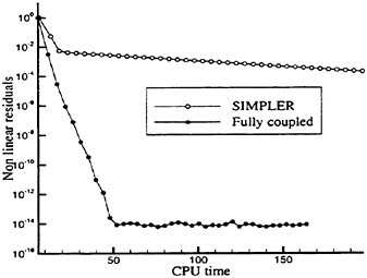
Figure 1: comparison between fully coupled and SIMPLER algorithm for symmetrical flow
2 Governing equations, turbulence model
The convective form of Reynolds Averaged Navier-Stokes Equations are written through partial transformation from cartesian space (x1, x2, x3) to curvilinear space (ξ1, ξ2, ξ3) fitted to the hull and the free surface at each time. Free surface elevation, the 3 cartesian velocity components (ui), pressure (p) including gravitational effects (ρgx3) and turbulent kinetic energy ![]() are the dependant unknowns.
are the dependant unknowns.
Mean momentum transport equations are written in the moving referential attached to the hull :
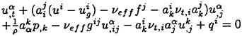
(1)
Where ai is the contravariant basis, gij the contravariant metric tensor, fi the control grid function and ![]() the grid velocity which traduces the displacement of the mesh. Inertia forces due to non galilean referential (gyration, accelerated translation) are taking into account in the qi terms. In translation case (with or without drift angle) inertia forces are expressed as follows where Ua is the hull velocity:
the grid velocity which traduces the displacement of the mesh. Inertia forces due to non galilean referential (gyration, accelerated translation) are taking into account in the qi terms. In translation case (with or without drift angle) inertia forces are expressed as follows where Ua is the hull velocity:
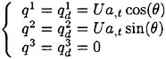
(2)
In gyration case, inertia forces must include Coriolis and centrifugal forces:
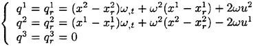
(3)
Where ω is the hull rotation velocity and ![]() the rotation center location (figure 2).
the rotation center location (figure 2).
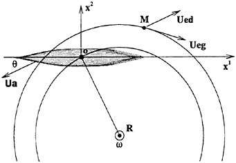
Figure 2: attached referentials for gyration and drift cases
Mass conservation is expressed as the classical continuity equation:
(4)
To close the equation set we used a classical k−ω turbulence model proposed by Wilcox [12], [13], [14], introducing a specific dissipation rate ![]() without low Reynolds formulation requirement. Transport equation of turbulent kinetic energy and dissipation rate are written as follows:
without low Reynolds formulation requirement. Transport equation of turbulent kinetic energy and dissipation rate are written as follows:
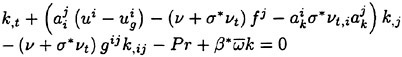
(5)
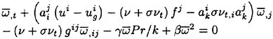
(6)
with:
(7)
and:
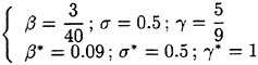
(8)
3 Free surface conditions
Free surface boundary conditions are one kinematic condition, two tangential dynamic conditions and one normal dynamic condition. The kinematic condition, coming from the continuity hypothesis, expresses that the fluid particles of free surface stay on it:
(9)
where bi are the bi-dimensional contravariant basis.
Dynamic conditions are given by the continuity of strains at the free surface. If the pressure is assumed to be constant above free surface, normal dynamic condition is:
(10)
where γ is the surface tension coefficient (that is a physical way to smooth free surface near the hull) and r the free surface medium curvature radius. Tangential dynamic conditions are simply given by a linear combination of first order velocities derivatives:
(11)
4 Discretization
General discretization method is based on second order (in space and time) implicit finite differences. Discrete unknowns are distributed on a structured curvilinear grid fitted to the hull and the free surface. Velocity cartesian components, kinetic turbulent energy, and specific dissipation rate are located on the grid nodes. Pressure is located on the center of each elementary volume and free surface elevation is located on the center of free surface interfaces.
Convection terms are computed using an upwind second order scheme that needs a 13 nodes cell. Diffusion terms need 7 nodes for second order derivatives and 12 nodes to express cross second order derivatives (equation 1) while pressure gradient requires 8 nodes for each component [1], [2].
Concerning free surface calculation, it has been shown that classical way using normal dynamic condition as Dirichlet condition on the pressure and uncoupled kinematic equation as transport equation to compute free surface elevation induces some problems connected to difficulties to exactly solve mass conservation under free surface [2]. Efficient solution consists in using fully coupled algorithm [2] that requires at each iteration the linear solution of mean momentum equations, continuity equation and whole boundary conditions including free surface condition. Unfortunately the most efficient iterative algorithms (CGSTAB+ILU, Multigrid) are unable to invert this system because of the very bad matrix conditionning. The solution consists in modifying the system using free surface boundary conditions to express the flux through free surface. In this case, conditionning number decreases and fully coupled system becomes invertible by iterative algorithms (figure 3). Resulting linear system for velocity (U) and pseudo velocity (Ũ) components, pressure (P) and free surface elevation (H) is written as follows:
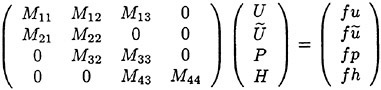
(12)
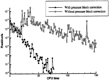
Figure 3: CGSTAB+ILU convergence using modified and non-modified pressure block
Two recent iterative methods have been tested in this paper. First method consists in an improvment of CGSTAB algorithm using matrix preconditionning [11]. Second method is based on linear full multigrid algorithm. Figure 4 presents the convergence of the
two algorithms solving typical fully coupled system. We can see that full multigrid seems more efficient than CGSTAB, nevertheless it can be noticed that this result needs a lot of benches to adjust multigrid parameters (prolongation operator, restriction operator, smoothing operator, cycles schemes) and is not easily usable for practical computations.
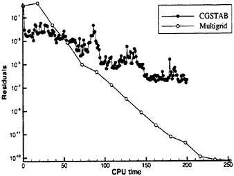
Figure 4: Comparison between CGSTAB and full multigrid algorithms
5 Periodic boundary conditions and topological domain
Numerical algorithms are optimized for structured grid. In this paper O-O topology (figure 5) has been chozen in order to accurately describe velocitity profiles in the boundary layer (high concentration near the wall) without unprofitable concentration on the upwind symetry plane like in H-O topology for exemple. The only default of such a grid is a lack of nodes in the wake. Definitively the best topoloy seems to be C-O topology but unfortunately it is not tested in this paper.
In the symmetrical flow case and for classical topologies (that means H-H, H-O, O-O etc…) each topological boundary corresponds to physical boundary conditions. In the non-symmetrical flow case (gyration or drift angle case) the problem is that some topological boundaries are not physical boundaries and classical boundary conditions can not be applied. On such boundaries (i=1, i=imax, k=kmax for O-O topology) periodic boundary conditions have to be applied (figure 5). This kind of conditions allowing to solve Navier-Stokes and continuity equations on topological boundaries located inside the interior of the physical domain can be considered as multiblock junction boundaries.
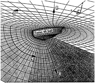
Figure 5: O-O Grid topology around Series 60 hull
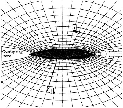
Figure 6: Overlapping technique using O-O topology (top view)
First method to solve this problem comes from multiblock theory: grid overlapping (figures 6, 7) allowing to solve governing equation on the junction is used and boundary conditions are expressed as follows:
(13)
where gi are the two overlapped grids, ibi the indice corresponding to the topological boundary of grid gi, nover the number of indices overlapped, δi=1 if ibi is a maximum and δi=−1 if ibi is a minimum.

Figure 7: Overlapping technique using O-O topology (front view)
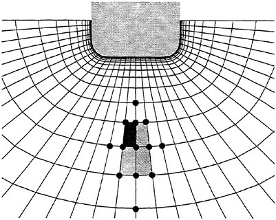
Figure 8: Special discretization cell on the junction
This method appears very attractive because of the easiness to code it using classical boundary conditions. Unfortunately the two classical ways to implement these conditions (implicit or explicit) gives poor numerical performances.
Explicit way, consisting in solving one block before other and iterate is the simplest way but convergence rate of this method, due to a weak coupling between the two block is very poor and numerical process usually ends to an unacceptable saturation of convergence level. Theoretically implicit way allows to preserve convergence rate but using fully coupled algorithm full linear system becomes very hard to invert and needs a lot of Multigrid cycles or CGSTAB iterations. The reason of that seems due to the presence of metric singularity line (i=1, k=kmax) where jacobian of transformation is equal to zero. This singularity is not a problem in symmetrical case because it corresponds with physical boundary but, using overlapping, it becomes in the inner domain just on a cusp location producing poor conditionning in linear system.
Another method consists in using joined grids (without overlapping) and developping special schemes and particular linear solvers (figure 8). Continuity equation (pressure equation) and transport equations (momentum equations, transport for turbulence modelisation, kinematic boundary conditions) require some special developments to allow informations to cross topological boundaries. It is clear for exemple in figure 8 that convection-diffusion cell in the boundary (k=kmax) requires informations on the two sides of boundary staggering totaly schemes numerotation. Consequence is that all the algorithms have to be modified building a correspondance between virtual location “out” of topological domain (for example M(i, j, k) with i>imax) and physical location.
Concerning the values located on the nodes (velocity components, turbulence kinetic energy, turbulence dissipation rate etc…) if Mv(iv, jv, kv) and Mp(ip, jp, kp) are respectively the virtual and actual curvilinear coordinates of nodes M the transformation rules are the following:
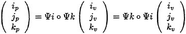
(14)
where Ψi and Ψk are the transformation used respectively when Mv overrun i or k authorized values: i ∈ [1, imax] and k ∈ [1, kmax]:

(15)
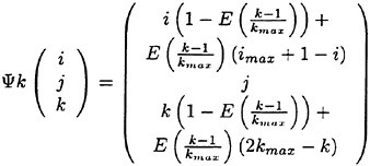
(16)
We can note naturally that if (i, j, k) is in the physical domain: Ψi(i, j, k)=Ψk(i, j, k)=(i, j, k).
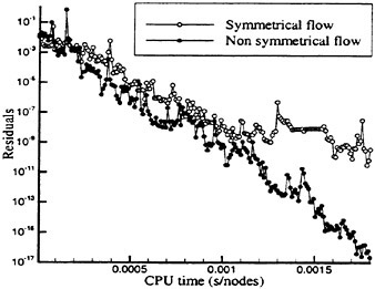
Figure 9: Linear solver convergence on fully coupled system for symmetrical and non symmetrical flows
Concerning the values located at the centre of each elementary volume (pressure) transformations between virtual center Cv(iv, jv, kv) to physical center Cp(ip, jp, kp) are given as follows
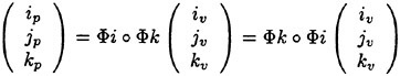
(17)
with:
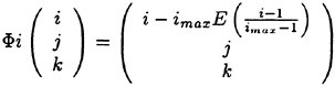
(18)
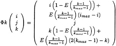
(19)
This modifications are easy to describe, nevertheless they concern many numerical details during discretization or linear system solving processes. Finally as we can show on the figure 9 this method to solve non-symmetrical flows is very efficient since the convergence during linear solver iteration is faster than for symmetrical flows.
6 Gyration specific problems
Once the problem of topological boundaries connecting solved next step is to consider that calculation past ship with drift angle and calculation with gyration motion are very similar: working in relative referential moving with the hull, Coriolis and centrifugal forces have to be added as source terms in momentum equation. This section shows that gyration case is quite more difficult and requires some numerical cautions.
In this relative referential, relative velocity field traducing flow at rest (without hull effects) is written as follows for the drift case (Ued in figure 2):
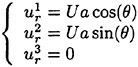
(20)
and:
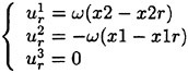
(21)
in the gyration case (Ueg in figure 2).
In both cases these velocity fields have to verify momentum and continuity equations (1) and (4) with pressure gradient and turbulent viscosity equal to zero. For uniform velocity field (20) verification is evident because of the annulation of convection and diffusion terms, we obtain respectively for momentum and continuity equations:

(22)
For velocity field coming from gyration case verification of continuity equation is quite easy and momentum equations gives:
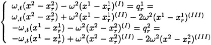
(23)
where Coriolis (III) terms are exactly balanced by centrifugal terms (II) for half part and convection terms (I) for other part.
Problems appear considering discretization of these equations. In the drift case, due to the uniformity of velocity field, discrete momentum and continuity equations are verified exactly. Unfortunately in the gyration case two problems appear due to linearization and discretization.
First problem is shown considering that discrete derivatives of velocity field are unable to give exactly rotation velocity:
(24)
(25)
where Δ is a general discretization operator used in the present formulation.
A solution consists in adding source terms in order to balance convection residuals. This consistent terms (they converge to zero when discretization step is tending to zero) are calculated as follows:
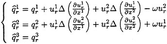
(26)
Second problem is due to convection terms linearization: generally convection velocities are expressed as previous non-linear iteration velocities and convection terms are of course (because it is impossible for non-linear terms) not totally implicit and verification of momentum equations requires good convergence on linear and non-linear processes. For this reason unsteady flow computation past a hull in gyration is very slow.
7 Calculation past Series 60
We present here first numerical results for both drift angle and gyration cases. Calculation are performed on a Series 60 Cb=0.6 hull for a Reynolds number Rn=Ua.l/ν=5.3.106, a Froude number Fn=![]() and a Bond number which traduces surface tension effects Bn=ρgl2/γ=1.3106, where l is the boat length. A O-O tolpology grid (figure 5) is used in every calculation but for CPU time reason grid sizes are not the same: finest grid has 2×89×73×33=428802 nodes and coarser grid has 2×57×49×33=184338 nodes. The utilization of these two grids is specified in the following sections. k−ω turbulence model [12] is used without wall function which requires a great concentration near the hull: first grid point is located at s/l=10−5 where s is the curvilinear coordinate from the hull.
and a Bond number which traduces surface tension effects Bn=ρgl2/γ=1.3106, where l is the boat length. A O-O tolpology grid (figure 5) is used in every calculation but for CPU time reason grid sizes are not the same: finest grid has 2×89×73×33=428802 nodes and coarser grid has 2×57×49×33=184338 nodes. The utilization of these two grids is specified in the following sections. k−ω turbulence model [12] is used without wall function which requires a great concentration near the hull: first grid point is located at s/l=10−5 where s is the curvilinear coordinate from the hull.
Calculations are performed during 500 time iterations with a non dimensional time step τ=Uaδt/l=0.025 for all grids. Starting calculations with the final boat speed creates a shock on free surface and requires high sub-relaxation coefficient drastically reducing convergence performances. In order to avoid this problem calculations simulate exactly a towing tank test: during a first stage the hull is in uniform acceleration up to the nominal velocity and then velocity is constant.
A very important problem in free surface flows modelisation concerns wave-breaking phenomena. In many cases, computations stop because of wave breaking. Questions are: has wave breaking a numerical or physical origin? How to numerically detect wave breaking? How much energy dissipation through wave breaking? are discussed in the following section.
7.1 Wave-Breaking modelisation
An important topic for the future concerns the problem of bow wave-breaking that appears fundamental for incidence or gyration effects calculations. First question is to determine the origin of this phenomenon: physical origin or numerical origin?
Two phenomena coexist: the problem of plunging or spilling breaker and the problem of compatibility between no slip boundary condition on the body and kinematic condition on the free surface.
Astonishingly spilling breaker does not seems to be a difficulty: 2D calculation shows that numerical dissipation on the free surface increases with free surface slope and prevents free surface to achieve breaking slope. In this case numerical dissipation acts like breaking energy dissipation. The problem of spilling breaker and jet on the bow is more problematic, the fast increase of vertical velocity on the free surface cannot be balanced by numerical dissipation and ends to the divergence of calculation. Computation of turbulent flows past hulls in incidence or in gyration requires first to detect where wave-breaking could occur and second to specify how much energy, corresponding to breaking energy, has to be absorbed to numerically avoid wave-breaking.
In the present calculation a wave-breaking criterion based on free surface curvature is used. This criterion published by Subramani et al [18] fixes the limiting
value of |κh| where κ is the free surface curvature and h the free surface elevation for a wave not to break:
(27)
Figures 10 and 11 show the values of |κh| parameter for flows past Series 60 with drift angle and in gyration case (see 7.2 and 7.3 for flow parameters). Black region is for |κh|<0.15 and white region for |κh|>0.4.
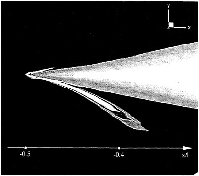
Figure 10: wave-breaking criteria for drift angle case
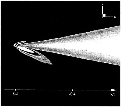
Figure 11: wave-breaking criteria for gyration case
In both calculations the criteria (27) seems to lax to avoid numerical wave-breaking. We proposed here to use
(28)
for wave-breaking criteria (white region on figure 10 and 11).
Next question is how to absorb wave-breaking energy? An efficient method is to modified normal dynamic condition adding damping pressure:
(29)
with:
(30)
Problem is to adapt ψ function to absorb breaking energy quantity only [19].
This absorption method has not been developped today. In this paper, after wave-breaking detecting (28) a free surface limitation to breaker detection level is applied.
The problem of compatibility between kinematic and no-slip conditions appears very close to the hull for large Reynolds number (Rn>107) and the physical contradiction can be solved by the forsaking of continuity hypothesis that is out place in this context. Mathematically, displacement of contact point is asymptotically ensured by tangency of the hull with free surface. In any case, free surface elevation unknowns have to be located on the contact point. Nevertheless a free surface formulation allowing an accurate mass conservation and a strict discretization of free surface conditions (and only free surface conditions that is not always done) avoids a lot of numerical problems assimilated by error to wave-breaking.
7.2 The drift angle case
We present here flow simulation past Series 60 with attack angle θ=5° on the finest grid. In the whole section experiments are due to J.Longo and F.Stern from Iowa university [5].
Figure 12 shows calculated wave field around the hull in comparison with experiments. General agreement is satisfactory: bow and stern local free surface on pressure side or succion side has good amplitude and computed and experimental wave patterns are very similar. Nevertheless computed wavefield presents a today most classical default of three-dimensional free surface viscous flows: An important wave damping appears moving away from the hull in spite of full second order discretization due to insufficient longitudinal grid resolution. Agreement with
experiments become worse far to the hull and Kelvin diedron is absent of the calculation. Grid resolution is frequently invoked but in order to improve numerical results high order (third and fourth) finite differences schemes have been tested for kinematic condition only: results has been astonishingly similar. The conclusion is that this important damping is not due to free surface condition discretization but rather to convection and above all to continuity equation that is to say pressure equation discretization.
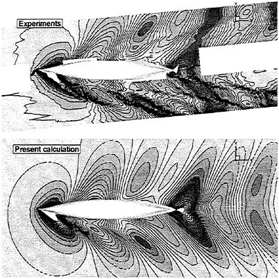
Figure 12: wave field for Fn=0.316 and Rn=5.3.106
Figure 13 shows free surface elevation along the hull on the pressure and succion sides. We can see that numerical damping above described does not exist in this picture and appears far to the hull (figures 14 to 21). On the pressure side wave height is well calculated: first crest on the bow has satisfactory amplitude and agrees better with experiments than A.Di Mascio et al Navier-Stokes calculation [3] in spite of present coarser grid resolution. On the other hand stern crest is overestimated by present formulation that is not clearly explained. On the succion side we have the same conclusions: particular shape of bow crest with two peaks near is well computed.
Figures 14 to 21 present a free surface elevation comparison between numerical calculation and experiments for various values of y/l on the pressure and succion sides. These pictures show the consequences of numerical damping: near the hull on the pressure or succion side (figures 17 and 18) for y/l=±0.15 numerical results are in good agreement with experiments (as along the hull figure 13) but far to the hull for y/l=±0.2; ±0.25 (figures 15, 16, 19 and 20) calculations show significant loss of amplitude and farther for y/l=±0.3 (figures 14 and 21) difficulties to predict wavelength.
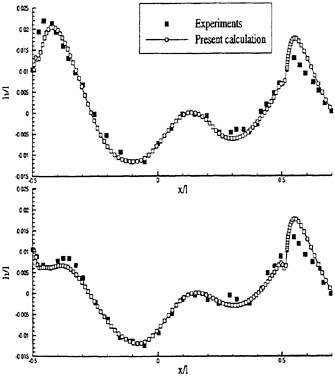
Figure 13: free surface elevation along the hull (pressure side on the top and succion side on the bottom)
Figure 28 in color shows variation of velocity components in 11 sections from x/l=−0.5 to x/l=0.5 (step equal 0.1). Nevertheless, for this attack angle, experiments concerning local velocity field does not exist. J.Longo and F.Stern presents this kind of results but at 10° of incidence [5]. In their paper a detached vortice in the stern region of the succion side is well presented [5]. Present calculation at 5° of incidence shows a beginning of separation in this region but with weaker intensity because of the difference between experiments and calculation attack angle. Future computation or experiments for the same attack angle will be certainly fruitful for a good interpretation of numerical results.
Last numerical results concern evolution of forces integration on the hull during numerical simulation. Fp is the force due to pressure integration on the hull, Fd is the drag due to viscous stress, and Mp and Md the corresponding moment at coordinates (0,0,0). Fxp and Fyp are the components of Fp on the x1 and x2 axis respectively, Fxd and Fyd the components of Fd and Mzp and Mzd the projection of Mp and Md on x3 axis (figure 2). We define also non-dimensional
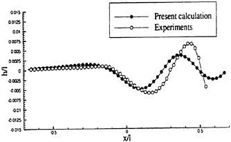
Figure 14: free surface elevation for y/l=−0.3
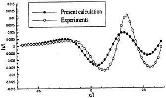
Figure 15: free surface elevation for y/l=−0.25
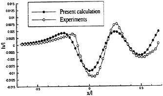
Figure 16: free surface elevation for y/l=−0.2
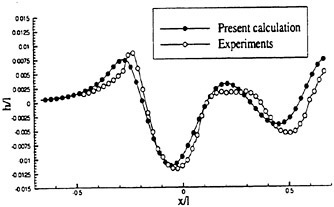
Figure 17: free surface elevation for y/l=−0.15
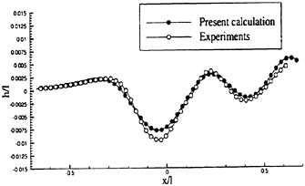
Figure 18: free surface elevation for y/l=+0.15
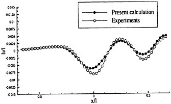
Figure 19: free surface elevation for y/l=+0.2
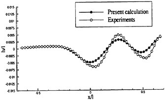
Figure 20: free surface elevation for y/l=+0.25
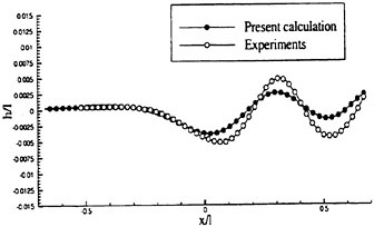
Figure 21: free surface elevation for y/l=+0.3
coefficients as follows:
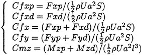
(31)
with:
(32)
(33)
(34)
(35)
where n is the external normal to the hull, and σ the stress tensor defined on the hull by:
(36)
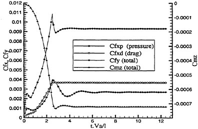
Figure 22: Forces integration during the simulation
Figure 22 shows several non-dimensional resistance coefficients during the simulation, we can note relaxation oscillations of Cfxp, Cfy, Cmz. These oscillations of pressure integration due to initial acceleration slope may be observed during towing tank test. J.V.Wehausen [20] has studied this phenomenon analytically on a cylinder under perfect flow free surface (potential flow). The decomposition of the two first order terms of wave resistance displays oscillations with a period t0 according to ![]() which gives in non-dimensional variables T0=8πFn2 with T0=t0Ua/l. This formulation of oscillations period giving T0=2.51 is in good agreement with calculation presented in figure 22.
which gives in non-dimensional variables T0=8πFn2 with T0=t0Ua/l. This formulation of oscillations period giving T0=2.51 is in good agreement with calculation presented in figure 22.
Figure 22 shows also that viscous and pressure forces converge to steady values in accordance to experimental values listed in the following table. It can be notice that experimental results [5] are obtained with sinkage, trim and heel free for a Reynolds number equal to 5.3.106 and a Froude number equal to 0.319.
|
|
Cfx |
Cfy |
Cmz |
|
Experiments |
6.6.10−3 |
10.6.10−3 |
−0.73.10−3 |
|
Calculation |
6.4.10−3 |
9.3.10−3 |
−0.72.10−3 |
7.3 The gyration case
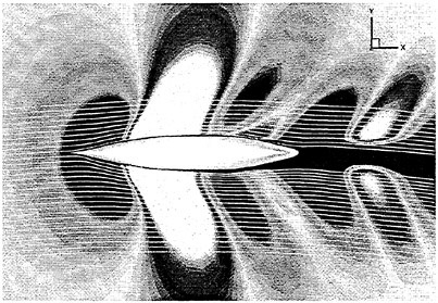
Figure 23: Modulus of velocity and streamlines on the free surface for Rg/l=11.5
For the gyration case, boat velocity is the same that for drift angle case: Froude number Fn=0.316 and Reynolds number Rn=5.3.106. The rotation velocity Ω (in radians/s) is choose according to Ωl/Ua=8.73.10−2 involving a curvature radius Rg/l=Ua/(Ωl)=11.5. The rotation axis is vertical (of course) including point R(0, −Rg, 0) (figure 2) and the boat is fixed in all the degrees of freedom.
Figure 23 shows the modulus of the velocity minus modulus of pure rotation velocity on the free surface associated to streamlines in the referential moving with the hull. We can see that general streamlines are circles centered on R deviated by the hull. Velocity modulus allow to present both gravitational
and viscous effects. Oscillations of velocity modulus, decrease of velocity on the hump of free surface and increase on the hollow are typically gravitational effects but on the other hand decrease of velocity on the boundary layer and the wake is viscous effects. Interaction between these effects as rotation of waves field or wake convected in the streamlines direction are well presented in figure 23.
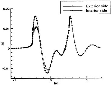
Figure 24: Free surface elevation on both sides of the hull for Rg/l=11.5
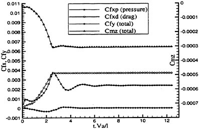
Figure 25: Forces acting on the hull during gyration for Rg/l=11.5
Figure 24 presents free surface elevation along both sides of the hull (internal side for y<0 and external side for y>0). Unfortunately experiments are not available for comparison with this kind of calculation, moreover it has to be noticed that in comparison with the solution for Rg/l → +∞ (that is to say for symmetrical flow without giration) [1], [2] free surface elevations for Rg/l=11.5 (present calculation) are very different. Non-dimensional amplitude of bow crest on the interior side is aproximately equal to 0.0165 but reaches only 0.011 on the interior side and 0.013 for symmetrical flow. Amplitudes of the hollow after the first crest are similar and it seems very difficult to characterize interior and exterior sides downstream x/l=0 in terms of free surface elevation.
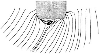
Figure 26: Transversal streamlines in x/l=−0.1 section
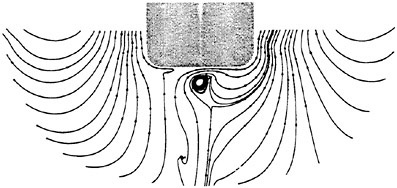
Figure 27: Transversal streamlines in x/l=0 section
Figure 25 shows forces acting on the hull during the acceleration stage (non-dimensional duration Τ =2.5) and the gyration. Notations are similar than for previous calculation with attack angle and forces present the same general evolution with a very distinct end of acceleration process. Differences can be noted for vertical momentum (Cmz) which is approximately two time smaller than for 5° of incidence and for transversal force (Cfy) which is almost zero at the end of computation. Converged values of forces after 500 time steps are summarized in the following table. These results cannot be compared today with experiments but will be useful for validation of other computation. Nevertheless a small increase of resistance (row 1) due to gyration can be observed comparing with experiments (row 3) and calculation (row 2) for Rg/l =+∞.
|
|
Cfx |
Cfy |
Cmz |
|
Cal. (1) |
6.1.10−3 |
1.4.10−5 |
−0.31.10−3 |
|
Cal. (2) |
5.7.10−3 |
0 |
0 |
|
Exp. (3) |
5.9.10−3 |
0 |
0 |
Figure 29 presents velocity components in various section from x/l=−0.5 to x/l=+0.5 with a step equal to 0.1. First remark is that general flow is fully non-symmetrical in spite of the important value of gyration radius and explains the increase of resistance comparing with symmetrical solution (Rg/l → +∞). As for the calculation with 5° incidence, a beginning of separation is perceptible for section x/l=−0.2, x/l=−0.1 and x/l=0 in the longitudinal velocity representation. Boundary layer growing on the stern region presents a topology radically different than for drift angle case: boundary layer thickness appears very uniform on a section (x/l=0.4) for gyration case and very non-symmetrical due to transverse convection for drift case. In fact gyration case is characterized by an inversion of transverse convection approximately for x/l=0 (due to absicea of rotation center R equal to zero) that is not true in the calculation with incidence.
Transversal streamlines (without longitudinal component) in two sections (x/l=−0.1 and x/l=0) are presented on figure 26 and 27. A large vortex appears near the keel when the flow crosses the bilge due for a part to the variation of general transversal convection in the longitudinal direction.
8 Concluding remarks
A numerical method solving Reynolds Averaged Navier-Stokes Equations and allowing to compute non-symmetrical turbulent flows past ship hull is presented here. Classical overlapping technics coming from multiblock solvers have been tested in order to transmit flow informations (mass and momentum conservation) through topological (but not physical) boundaries joining the two blocks (starboard and port). Unfortunately this method gives very slow convergence rate that suppress the benefit of fully coupled technics. Better way consisting in coding new schemes on and near the topological boundary and new specific linear solvers is developped here. In this case, the two parts of the grid are not overlapped and convergence rate in the whole domain appears better than convergence with symmetrical flow.
This method has been validated in two important cases for hydrodynamics point of view: ship moving with a non-zero attack angle and ship in rotating motion. In both case non-symmetrical flows and continuity of dependant unknows crossing boundaries are shown.
Concerning drift simulation general wave pattern shows a good agreement with experiments particularly on the bow wave where amplitude on the succion and pressure sides are good. Nevertheless important wave damping can be observed at a distance from the hull as usual using RANSE solver. Converged values of resistance coefficients are in very good accordance with experimental values.
Concerning gyration simulation, experimental values concerning local variables (pressure, velocity, free surface elevation) do not exist today and validations are not very easy. Nevertheless an increase of resistance can be observed comparing with symmetrical flow simulation.
Future work will consist in simulation of more complex non-symmetrical flows studying ships with high drift angle (allowing to compare with J.Longo et al local measurements at 10° [5]) or small gyration radius but this will be possible only using a robust wave-breaking modelisation.
Acknowledgments
Thanks are due to the French Ministry of Defense and to the “Bassin d’Essais des Carènes” which are supporting this work.
References
[1] B.Alessandrini, G.Delhommeau, “A multigrid velocity-pressure-free surface elevation fully coupled solver for turbulent incompressible flow around a hull calculation”, 9th International Conference on Numerical Methods in Laminar and Turbulent flow, Atlanta, July 1995.
[2] B.Alessandrini, G.Delhommeau, “A multigrid velocity-pressure-free surface elevation fully coupled solver for calculation of turbulent incompressible flow around a hull”, 21st Symposium on Naval Hydrodynamics, Trondheim, June 1996.
[3] A.Di Mascio, R.Penna, M.Landrini, E.F.Campana, “Viscous free surface flow past a ship in steady drift motion”, Workshop on Water Waves and Floating Bodies, Carry Le Rouet, March 1997.
[4] E.F.Campana, P.G.Esposito, R.Penna, “Numerical simulation of the drift motion of a ship”, Proc of the 20th O.N.R. Symposium on Naval Hydrodynamics, Santa Barbara, 1994.
[5] J.Longo, F.Stern, “Yaw effects on model-scale ship flows”, 21st Symposium on Naval Hydrodynamics, Trondheim, June 1996.
[6] Y.Toda, F.Stern, J.Longo, “Meanflow measurements in the boundary layer and wake and wave field of a Series 60 Cb=0.6 ship model, Part 1: Froude numbers 0.16 and 0.316”, Journal of Ship Research, Vol 36, No 4, pp. 360–377, 1992.
[7] J.Longo, F.Stern, Y.Toda, “Meanflow measurements in the boundary layer and wake and wave field of a Series 60 Cb=0.6 ship model, Part 2: scale effects on near field wave patterns and comparisons with inviscid theory”, Journal of Ship Research, Vol 37, No 1, pp. 16–24, 1993.
[8] J.Farmer, L.Martinelli, A.Jameson “Multigrid solutions of Euler and Navier-Stokes equations for a Series 60 CB=0.6, ship hull for Froude numbers 0.160, 0.220, 0.316”, CFD Workshop, Tokyo, March 1994.
[9] Y.Toda, F.Stern, J.Longo, “Mean flow measurements in the boundary layer and wake field of a Series 60 CB=0.6, ship model for Froude numbers 0.16 and 0.316”, IIHR report, 352, August 1991.
[10] Y.Toda, F.Stern, I.Tanaka, V.C.Patel, “Mean flow measurements in the boundary layer and wake field of a Series 60 CB=0.6 ship model with and without propeller”, Journal of ship Research, Vol 34, December 1990.
[11] H.A.Vorst, “Bi-CGSTAB: a fast and smoothly converging variant of Bi-CG for the solution of non-symetric linear systems”, J. Sci. Stat. Comp. vol 13, 1992.
[12] F.R.Menter, “Zonal two equation k−ω turbulence models for aerodynamics flows”, ΑΙΑA Paper, 93–2906, Fluid Dynamics Conference, Orlando, July 1993.
[13] D.C. Wilcox, “Multiscale model for turbulent flows”, AIAA Journal, Vol. 26, pp. 1211–1320, November 1988.
[14] D.C.Wilcox, “Reassessment of the scale-determining equation for advanced turbulence models”, AIAA Journal, Vol. 26, pp. 1299–1310, November 1988.
[15] M.S.Longuet-Higgins, “The instabilities of gravity waves of finite amplitude in deep water”, Part 1, Superharmonics, Proc. Royal Soc., Vol. 360 pp. 471–488, London, 1978.
[16] M.S.Longuet-Higgins, “The instabilities of gravity waves of finite amplitude in deep water”, Part 2, Superharmonics, Proc. Royal Soc., Vol. 360 pp. 489–505, London, 1978.
[17] W.K.Melville, “The instabilities and breaking of deep-water waves”, Journal of Fluid Mech., Vol 115, pp 165–185, 1978.
[18] A.K.Subramani, R.F.Beck, W.W.Schultz, “Suppression of wave-breaking in nonlinear water wave computations”, 13th International Workshop on Water Waves and Floating Bodies, Delft, March 1998.
[19] J.H.L.Kway, Y.S.Loh, E.S.Chan, “Laboratory study of deep-water breaking Waves”, Ocean Engng. Vol 25, No 8, pp. 657–676, 1998.
[20] J.V.Wehausen, E.V.Laitone, “Surface Waves”, Handbuch der Physik, Band IX, Strömungsmechanik III, Springer-Verlag, Berlin, pp 446–815, (1960).
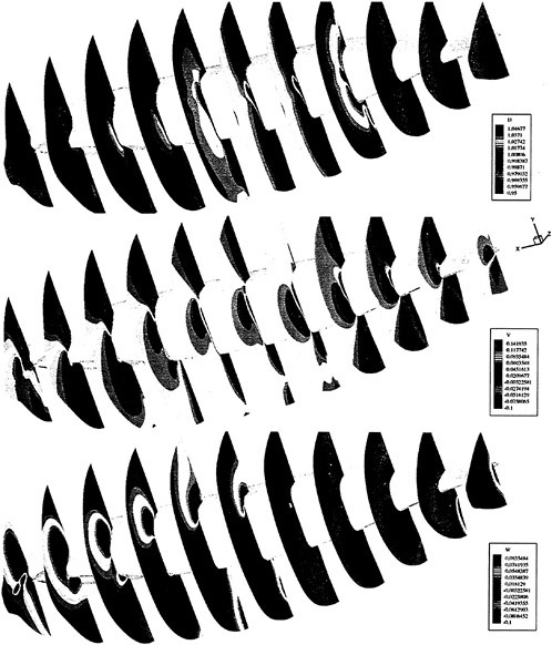
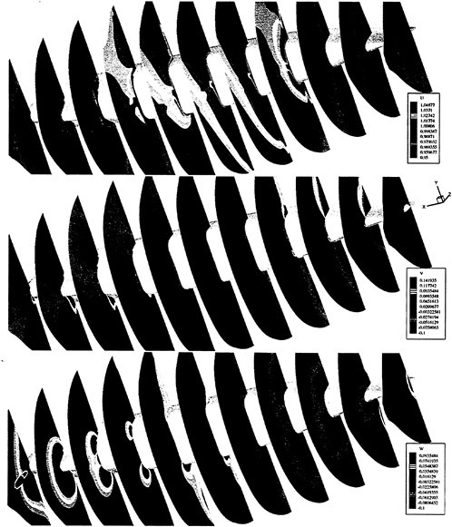
DISCUSSION
Η.Raven
Maritime Research Institute, The Netherlands
I am a bit puzzled by your finding that a fully coupled solution for velocity, pressure and wave elevation improves the convergence. In your equation (12), the last equation is entirely uncoupled, so Η can be found after solving for U, Û and P, without any approximation. So how can a coupled solution behave better?
AUTHORS’ REPLY
No reply from authors.
DISCUSSION
T.Hino
Ship Research Institute, Japan
In the wave breaking model proposed in this paper, the damping pressure is applied to absorb the wave energy associated with wave breaking. How does this model affect the flow field other than damping the local steep wave crests? In particular, how does the force acting on a ship hull vary with this breaking model? Also, do the computations reproduce the momentum loss beneath the free surface observed in the wake survey of ships with bow wave breaking?
AUTHORS’ REPLY
No reply from authors.
Numerical Simulation of Bow Waves
D.Dommermuth,1 G.Innis,1 T.Luth,1 E.Novikov,2 E.Schlageter,1 J.Talcott1
(1Science Applications International Corporation, 2University of California at San Diego, USA)
Abstract
A stratified-flow formulation is used to model nonlinear free-surface flows. The sharp interface of the air with the water is identified as the zero level-set of a three-dimensional function. The effects of surface tension are modeled as a source term that is concentrated at the air-water interface. The three-dimensional, unsteady, Navier-Stokes equations are expressed in primitive-variable form. A LES formulation with a Smagorinsky sub-grid-scale model is used to model turbulence, and an eddy diffusivity model is used to model mixing of air with water. The formulation is used to study bow-wave breaking on the DDG 5415. The ship is modeled using a body-force technique on a cartesian grid. The three-dimensional body-force is generated using a surface panelization of the entire ship, including the above-water geometry up to and including the deck. Numerical convergence is demonstrated using 128×128×129 and 256×256×257 grid points. The numerical results compare well to whisker-probe measurements of the free-surface elevation measured at the bow. However, a contact-line problem limits the application of the method to the bow region. In regions aft of the bow, the level-set function does not correctly rise up the side of the ship due to the no-slip condition on the hull. As a possible solution, the contact-line problem is reformulated using a Helmholtz decomposition of the wavy and vortical portions of the flow. The new contact-line formulation can be applied to viscous-flow simulations of surface ships.
1 INTRODUCTION
The free-surface disturbance near a naval combatant moving with forward speed is often characterized by steep and breaking waves. Spray sheets can form near the bow, as well as spilling and plunging breakers. For shovel-nosed bows, thin sheets of water can ride up over the bow and break. Along the sides of the ship, air is entrained near the crests of steep breaking waves and inside the turbulent boundary layer. At the stern, the free surface can separate near the transom. The traditional numerical approaches to this problem assume that the free surface is single valued and that there is no air entrainment. We consider here the application of a stratified-flow formulation to the study of surface ships. In regions where there is no air entrainment, the free surface is modeled as a sharp interface between air and water. In order to simplify the geometric modeling as much as possible, we also consider the application of a body force to impose boundary conditions on the ship hull. The initial boundary-value problem is formulated on a cartesian grid. The numerical results are promising, but there are still issues that need to be addressed.
Marker-and-Cell (MAC) techniques also model ship waves using a cartesian grid (see [9]). The evolution of the free surface is tracked in a Lagrangian frame of reference using markers. Some recent applications of this method, model the free surface as a two-layered fluid.
The body boundary condition is imposed using either no-slip or slip conditions. As reviewed by [9], the MAC method has been applied to many free-surface problems. However, at present, the MAC formulation is difficult to implement on a parallel computer.
The stratified flow formulation is described in §2. The body-force technique is described in §3. In §4, a contact-line formulation for unstratified flows is described. Some simple test cases are described in §6, and preliminary comparisons to model-test experiments of the DDG 5415 are described in §7.
2 FREE-SURFACE FORMULATION
Consider turbulent flow at the interface between air and water. Let ui denote the three-dimensional velocity field as a function of space (xi) and time (t). For an incompressible flow, the conservation of mass gives
(1)
ui and xi are normalized by Uo and Lo, which are the characteristic velocity and length scales of the body, respectively. On the surface of the moving body (Sb), the fluid particles move with the body:
(2)
where Ui is the velocity of the body.
Let Vℓ and Vg respectively denote the liquid (water) and gas (air) volumes. Following a procedure that is similar to [11, 13], we let ![]() denote a level-set function. By definition,
denote a level-set function. By definition, ![]() for x ∈ Vg and
for x ∈ Vg and ![]() for x ∈ Vℓ. The fluid interface corresponds to
for x ∈ Vℓ. The fluid interface corresponds to ![]() .
.
The convection and turbulent diffusion of ![]() is expressed as follows:
is expressed as follows:
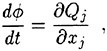
(3)
where d/dt=∂/∂t+ui∂/∂xi is a substantial derivative. Qj is a sub-grid-scale flux.
Let ρℓ and μℓ respectively denote the density and dynamic viscosity of water. Similarly, ρg and μg are the corresponding properties of air. The flow in the water and air is governed by the Navier-Stokes equations with modifications to account for turbulence:
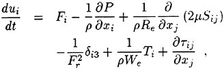
(4)
where Re=ρℓUoLo/μℓ is the Reynolds number, ![]() is the Froude number, and
is the Froude number, and ![]() is the Weber number, g is the acceleration of gravity, and σ is the surface tension. Fi is a body force that is used to impose boundary conditions on the surface of the body. Ρ is the pressure. Ti accounts for surface-tension effects. δij is the Kronecker delta symbol. τij is the subgrid-scale stress tensor and Sij is the deformation tensor:
is the Weber number, g is the acceleration of gravity, and σ is the surface tension. Fi is a body force that is used to impose boundary conditions on the surface of the body. Ρ is the pressure. Ti accounts for surface-tension effects. δij is the Kronecker delta symbol. τij is the subgrid-scale stress tensor and Sij is the deformation tensor:
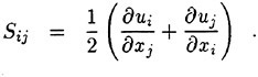
(5)
ρ and μ are respectively the dimensionless variable densities and viscosities:
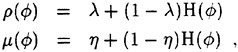
(6)
where λ=ρg/ρℓ and η=μg/μℓ are the density and viscosity ratios between air and water. The function ![]() accounts for the transition between water and air. For a sharp interface, with no mixing of air and water, Η is a step function.
accounts for the transition between water and air. For a sharp interface, with no mixing of air and water, Η is a step function.
Based on [1, 2], the effects of surface tension are expressed as a singular source term in the Navier-Stokes equations:
(7)
where κ is the curvature of the air-water interface expressed in terms of the level-set function:
(8)
Away from the fluid interface, the sub-grid scale stresses are modeled using a Smagorinsky sub-grid-scale turbulence model (see [12]).
(9)
cs is the Smagorinsky coefficient of turbulence. Δ is the grid spacing and |S| is the magnitude of the deformation tensor. The principal stress Tkk is absorbed into the pressure gradient term.
Similarly, the sub-grid-scale flux (Qj) of the level-set function ![]() is modeled using an eddy-diffusivity model (see, for example, [6]).
is modeled using an eddy-diffusivity model (see, for example, [6]).

(10)
![]() is a coefficient of turbulence associated with the mixing of air and water.
is a coefficient of turbulence associated with the mixing of air and water.
The pressure is reformulated to absorb the hydrostatic term:
(11)
where Pd is the dynamic pressure and Ph is a hydrostatic pressure term:
(12)
The divergence of the momentum equations (4) in combination with the conservation of mass (1) provides a Poisson equation for the dynamic pressure:
(13)
where Σ is a source term. Equation 13 is used to project the velocity onto a solenoidal field.
3 BODY-FORCE FORMULATION
With respect to the volume of fluid that is enclosed by the body (Vb), we define a function ![]() :
:
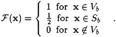
(14)
The function ![]() can be expressed in terms of a surface distribution of normal dipoles [8].
can be expressed in terms of a surface distribution of normal dipoles [8].
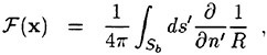
(15)
where n is the outward-pointing unit normal to the body, and R is a Rankine source, R=|x−x′|.
The function ![]() is used to construct a body force as follows:
is used to construct a body force as follows:
(16)
where cf is a friction coefficient.
A similar body force was constructed [7] in their numerical studies of flows in channels and over circular cylinders. However, formulation [7] differs from our own in several respects. First, unlike [7], a feedback loop is not included in equation 16. Second, the body force is distributed over the entire volume enclosed by the
body in equation 16, not just the surface of the body. This prevents the formation of the sloshing flows within the body. Finally, as discussed below, we use an adjustment procedure to reduce the formation of non-physical high-frequency waves within the computational domain.
Consider the solution to the following model equation to show the effect of the body force:
(17)
If initially ui=0, then for x ∈ Vb, the solution to this equation is
(18)
As t→∞, every point within the body moves with the body. In the inviscid limit, the normal component of velocity is continuous across the surface of the body.
Numerical simulations of free-surface flows are prone to developing non-physical high-frequency disturbances unless the flow field is given sufficient time to adjust (see [3]). The body-force term (see equation 16) is modified to reduce its initial impulse:
(19)
where A is an adjustment function:
(20)
To is the adjustment time. The adjustment function smoothly increases to unity from its initial value of zero. As shown by [3], this smooth transition reduces the generation of non-physical high-frequency waves.
As constructed, the region over which the force Fi is applied moves instantaneously with the body, but the actual fluid particles inside of the body smoothly accelerate from rest to full speed. The advantage of this technique is that the initial impulse of the body’s motion is reduced due to the influence of the adjustment function.
4 CONTACT-LINE FORMULATION
Viscous formulations of free-surface flows are problematic for surface-piercing bodies. For primitive-variable formulations of the Navier-Stokes equations, the no-slip condition that is imposed on the body inhibits the rise of the free surface along the side of the hull. For unstratified flows, it is possible to eliminate this confluence of boundary conditions by decomposing the flow into two parts: an irrotational portion and a vortical portion. The vortical portion of the flow is used to enforce the no-slip condition on the hull, and the irrotational portion of the flow is used to implement the free-surface boundary conditions. At present, we have been unable to derive a contact-line formulation that is suitable for stratified flows with no-slip conditions on the hull. For no-flux conditions on the hull, the free surface is free to rise up the side of the hull whether or not the flow is stratified.
Based on [4], the following Helmholtz decomposition is invoked for unstratified flows:
(21)
where ![]() is a velocity-potential which describes the irrotational flow and Vi is a solenoidal-field which describes the vortical flow such that
is a velocity-potential which describes the irrotational flow and Vi is a solenoidal-field which describes the vortical flow such that
(22)
(23)
where ∇2 is the Laplace operator. Since ![]() satisfies Laplace’s equation and the divergence of
satisfies Laplace’s equation and the divergence of
the rotational field Vi is chosen zero, the total velocity field ui conserves mass. The potential ![]() models the effects of waves, whereas the solenoidal velocity field Vi models the hull boundary layer and turbulence.
models the effects of waves, whereas the solenoidal velocity field Vi models the hull boundary layer and turbulence.
Based on this Helmholtz decomposition of the velocity field, the total-pressure Π is defined in terms of a vortical pressure Ρ and an irrotational pressure, as follows:
(24)
The vertical coordinate z is positive upward, and the origin is located at the mean free surface. The density, ρ=1, is constant for unstratified flows.
Substituting these decompositions (21 & 24) into the Navier-Stokes equations gives
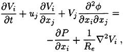
(25)
The divergence of the momentum equations (25) used in combination with the mass-conservation equations (22 & 23) can be used to derive a Poisson equation for the vortical pressure:
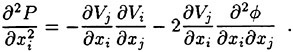
(26)
The vortical pressure is also subject to a solvability condition due to the imposition of Neumann boundary conditions.
The Helmholtz decomposition of the velocity field requires that two kinematic boundary conditions be imposed on the free surface. One expedient boundary condition that can be specified is that the normal component of the rotational velocity is zero on the free surface:
(27)
where z=η(x, y, t) is the free-surface elevation and ni is the unit normal on the free surface. The preceding constraint imposed on the rotational velocity field means that the evolution of the free-surface elevation is entirely prescribed in terms of the free-surface elevation and the velocity potential, as follows:
(28)
where everything is evaluated on the exact position of the free surface, z=η.
As shown by [4], the normal stress on the free surface must balance with the atmospheric pressure and the surface tension. Since it is difficult to resolve the free-surface boundary-layer at full-scale Reynolds numbers, a boundary-layer approximation is invoked:
(29)
where Pa is the atmospheric pressure due to wind forcing, d/dt=∂/∂t+ηt∂/∂z is a substantial derivative. The implications of equation 29 are discussed in [4].
On the ship hull, the velocity potential is used to enforce the normal velocity condition, and the solenoidal field is used to enforce the tangential velocity conditions, as follows:
(30)
(31)
where, here, ni is the unit normal on the ship hull. Equation 30 is the inviscid formulation of the hull boundary condition. If there is no vorticity (Vi=0), then the preceding formulation reduces to the nonlinear potential-flow around a body moving with forward speed. If there is
vorticity, the effects are felt in the inviscid portion of the flow through the vortical pressure term (P) in the normal-stress condition (29).
With the preceding formulation, the free surface is free to rise up the hull. Along the contact line, there is a discontinuity in the solenoidal velocity field that is similar to a lid-driven cavity flow. Suppose the hull is wall-sided and the free-surface is horizontal and rising vertically up the hull. By equation 27, the vertical component of the solenoidal velocity field is zero at a point on the free surface and slightly off the hull. On the hull, the vertical component of the solenoidal velocity field is nonzero by equation 31. This confluence of boundary conditions is the same as a lid-driven cavity flow. On the surface of the lid, the tangential velocity is nonzero, whereas on the walls of the lid, the velocity is zero.
5 NUMERICAL FORMULATION
The Navier-Stokes equations, and the boundary and initial conditions are discretized using 2nd-order finite differences. A fully-staggered grid is used in the numerical simulations. The grid can be stretched along the cartesian axes. The Navier-Stokes equations (4) and the level-set equation (3) are integrated with respect to time using a third-order Runge-Kutta scheme. Based on equation 13, the pressure is used to project the velocity onto a solenoidal field (see [4]). A solvability condition is enforced for the pressure. A multigrid solution scheme is used to solve the three-dimensional Poisson equation for the pressure. Based on [1], a mollified step function is used to model the singular surface-tension term (7). The hydrostatic contribution (12) is integrated analytically. No-flux boundary conditions are imposed at the bottom and top of the computational domain. The sides of the computational domain are periodic. The numerical algorithm has been implemented using high performance fortran.
6 NUMERICAL TESTS
As test cases of our numerical scheme, we have considered analytic solutions to Poisson’s equation, the evolution of a small-amplitude standing wave, and the flow around a sphere.
The analytic solution to Poisson’s equation tests the accuracy and efficiency of the multigrid solver. Based on these tests, the accuracy is second order. Table 1 summarizes the performance of the multigrid solver on a Cray T3E parallel computer. Three different grid sizes are considered: 643, 1283, and 2563 grid points. The cpu times are based on solving a Poisson equation with variable coefficients to machine accuracy. As shown in Table 1, as the number of cpu nodes increases for a fixed grid size, performance eventually degrades due to communication costs, but only for problems where the grid size is small compared to the number of nodes. For a fixed number of cpu nodes, the communication costs are significantly reduced (on a relative basis) as the number of grid points are increased. As a result, for 32 cpu nodes, it takes much less than eight times longer to solve the 1283 problem than the 643 problem.
Table 1. CPU seconds required to solve Poisson’s equation.
|
Grid Points |
Cray T3E Nodes |
||||
|
8 |
16 |
32 |
64 |
128 |
|
|
262,144 |
7.73 |
4.97 |
3.79 |
3.80 |
5.80 |
|
2,097,152 |
- |
25.8 |
14.7 |
9.40 |
9.25 |
|
16,777,216 |
- |
- |
96.4 |
50.8 |
30.7 |
The standing-wave problem tests the ability of the numerical scheme to model wave dispersion. The flow around a sphere illustrates the application of the body-force technique. Details of these tests are available upon request. Comparisons to model-test experiments of the DDG 5415 are discussed in the next section.
7 NUMERICAL RESULTS
As a demonstration of the level-set formulation and the body-force technique, we pre-
dict the free-surface disturbance near the bow of the DDG 5415 moving with forward speed. The experiments were performed at the David Taylor Model Basin (DTMB), and are available via the world wide web at http://www50.dt.navy.mil/5415/. Two Froude numbers were studied at DTMB. The results presented here correspond to the high speed case. For this case, a thin sheet forms near the bow. The leading edge of the sheet separates from the bow and breaks up into spray. Air is entrained and splash up occurs where the sheet reenters the free surface.
Based on the speed (Uo=6.02 Knots) and the length (Lo=5.72 m) of the model, the Reynolds and Froude numbers are Re=1.8×10⁷ and Fr2=0.41. The effects of surface tension are not included. The density ratio of air and water is λ=0.0012 and the ratio of the dynamic viscosities is η=0.018.
In regard to the numerical parameters, we use a friction coefficient cf=500 in the body-force term (16). The Smagorinsky coefficient is cs=0.0125 and the eddy diffusivity is ![]() =0.025. The adjustment time is To=0.20. The length and width of the computational domain are L=2 and W=1.28. The height of the air above the mean free-surface is h=0.12 and the depth below the mean free-surface is d=1.0. Two grid resolutions are used: 512×256×257 and 512×128×129. The grid is stretched along the y− and z-axes. For the highest grid resolution, the smallest grid spacing is 8.8×10⁻⁴ along the y-axis and 8.4×10⁻⁴ along the z-axis. The grid spacing (3.9×10⁻³) is constant along the x-axis. The ship is centered in the computational domain with the same fixed sinkage and trim as used in the experiments. In order to construct the body force term, the hull is panelized using approximately 4000 panels.
=0.025. The adjustment time is To=0.20. The length and width of the computational domain are L=2 and W=1.28. The height of the air above the mean free-surface is h=0.12 and the depth below the mean free-surface is d=1.0. Two grid resolutions are used: 512×256×257 and 512×128×129. The grid is stretched along the y− and z-axes. For the highest grid resolution, the smallest grid spacing is 8.8×10⁻⁴ along the y-axis and 8.4×10⁻⁴ along the z-axis. The grid spacing (3.9×10⁻³) is constant along the x-axis. The ship is centered in the computational domain with the same fixed sinkage and trim as used in the experiments. In order to construct the body force term, the hull is panelized using approximately 4000 panels.
The free-surface elevation was measured at DTMB using a whisker probe. Twenty-one transverse cuts were performed near the bow, extending from x=0 to x=0.178 in dimensionless units. The whisker probe measures the highest point of the free surface. In regions where there is wave breaking, the whisker probe measures the top of the breaking wave.
Figure 1 compares profile and whisker-probe measurements to the numerical predictions. The figures show the points where body forces are applied. The outline of the hull is also shown. The numerical simulations are compared to the profile measurements on the hull and the whisker-probe measurements near the hull. Two grid resolutions are shown: 512× 128×129 and 512×128×129. The numerical results are for t=0.75. At this time in the numerical simulation, the ship has moved three-quarters of a boat length, and the flow is steady near the bow. At later times, the flow wraps around the periodic domain and contaminates the solution near the bow. Radiation and absorbing boundary conditions are currently being investigated to eliminate this problem.
For x≤0.0533, the numerical simulations are in good agreement with the whisker-probe measurements. The surface profile is not predicted as well because the thin sheet on the hull is not resolved well by either the low or high resolution grids. For 0.0533≤x≤0.08, the numerical predictions agree well with both the whisker-probe and profile measurements. The high resolution grid predicts the profile better than the low resolution grid. The high resolution grid is also in better agreement with the whisker-probe measurements. In both numerical simulations the free-surface elevation is vertical near the hull. The high resolution grid captures the initial overturning and formation of a spray sheet. For x=0.0889, the sudden spike in the whisker-probe measurements shows where the whisker probe first came into contact with the top of the spray sheet. Due to inadequate resolution, neither grid captures the full extent of the spray sheet. As a result, the splash up that is evident for x≥0.116 is not captured by either numerical simulation. Outside of the spray sheet and splash region, the numerical simulations agree with measurements. We are currently investigating the application of a body-fitted coordinate system to improve grid resolution near the hull.
For x≥0.16, the surface profile as predicted
by the numerical simulations begins to diverge from the measurements. The free-surface elevation, which is extracted from the level-set function, is nearly tangent to the hull. In these regions, aft of the bow, the level-set function is not intersecting the hull properly. The rise and fall of the level-set function along the hull is impeded by the no-slip condition that is imposed on the hull. For unstratified flow simulations, this contact-line problem can be addressed using the Helmholtz formulation that is provided in §4. For unstratified flow simulations, we are currently investigating the applications of imposing no-flux conditions on the hull.
8 CONCLUSIONS
By modeling the air-water interface as a stratified flow with a very sharp interface, it has been been possible to circumvent some problems associated with conventional approaches, which generally assume that the free surface is single valued and do not account for air entrainment. The LES formulation permits the simulation of turbulent free-surface flows and the modeling of air entrainment. The body-force technique enables the enforcement of a hull boundary condition on a cartesian grid. However, the level-set function does not rise properly up the side of the hull. This contact-line problem can be eliminated in unstratified formulations by using a Helmholtz decomposition. For stratified flow simulations, a no-flux condition in lieu of no-slip will allow the level-set function to rise up the side of the hull.
ACKNOWLEDGEMENTS
DGD, GEI, TL, ECS, and JCT are supported by ONR under contract number N00014–97-C-0345. ΕΑΝ is supported by ONR under contract number N00014–97–1–0186. Dr. Edwin P. Rood is the program manager. The numerical simulations have been performed on the T3E computer at the Naval Oceanographic Office using funding provided by a Department of Defense Challenge Project.
REFERENCES
References
[1] BRACKBILL, J.U., KOTHE, D.B., & ZEMACH, C. 1992 A continuum method for modeling surface tension J. Comp. Phys. 100, 335–354.
[2] CHANG, Y.C., HOU, T.Y., MERRIMAN, B., & OSHER, S. 1996 A level-set formulation of Eulerian interface capturing methods for incompressible fluid flows J. Comp. Phys. 124, 449–464.
[3] DOMMERMUTH, D.G. 1994 The initialization of vortical free-surface flows J. Fluids Eng. 116, 95–102.
[4] DOMMERMUTH, D.G., GHARIB, M., HUANG, H., INNIS, G.E., MAHEO, P., NOVIKOV, E.A., TALCOTT, J.C., & WYATT, D.C. 1996 Turbulent free-surface flows: a comparison between numerical simulations and experimental measurements In Proc. Twenty-first Symp. on Naval Hydro., Trondheim, 249–265.
[5] DAI, Z., HSIANG, L.-P., FAETH, G. 1996 Spray formation at the free surface of turbulent bow sheets In Proc. Twenty-first Symp. on Naval Hydro., Trondheim, 197–211.
[6] EIDSON, T.M. 1985 Numerical simulation of the turbulent Rayleigh-Bénard problem using subgrid modeling J. Fluid Mech. 158, 245–268.
[7] GOLDSTEIN, D., HANDLER, R., & SIROVICH, L. 1993 Modeling a no-slip flow boundary with an external force field J. Comp. Phys. 105, 354–366.
[8] LAMB, H. 1932 Hydrodynamics. Dover, New York.
[9] MIYATA, H. 1996 Time-marching CFD simulation for moving boundary problems. In Proc. Twenty-first Symp. on Naval Hydro., Trondheim, 291–311.
[10] NOVIKOV, E.A. & DOMMERMUTH, D.G. 1997 Distribution of droplets in a turbulent spray Phys. Review E, 56(5), 5479–5482.
[11] OSHER, S. & SETHIAN, J.A. 1988 Fronts propagating with curvature-dependen speed: algorithms based on Hamilton-Jacobi formulations J. Comp. Phys. 79, 12–49.
[12] SMAGORINSKY, J. 1963 General circulation experiments with the primitive equations. I. The basic experiment Mon. Wea. Rev. 91, 99–164.
[13] SUSSMAN, M., ALMGREN, A.S., BELL, J.B., COLELLA, P., HOWELL, L.H., & WELCOME, M.L. 1996 An adaptive level-set approach for incompressible two-phase flows. In Proc. of the ASME Fluids Eng. Summer Meeting: Forum on Advances in Num. Modeling of Free Surface and Interface Fluid Dynamics. 355–360.
FIGURES
Figure 1a–t. Whisker-probe measurements. Transverse cuts of the free-surface elevation are shown from x=0 to x=0.169 in increments of Δx=0.00888. Small dots indicate points where a body force is applied. Solid, nearly vertical lines, show the outline of the hull, o’s denote DTMB profile measurements. Jagged solid lines are DTMB whisker-probe measurements. Numerical predictions at t=0.75 are symbolized by (- - - - - -) for 512×128×129 grid points and (- - - - - - - - -) for 512×256×257 grid points. All offsets are normalized by ship length.
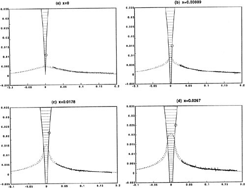
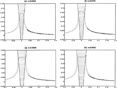
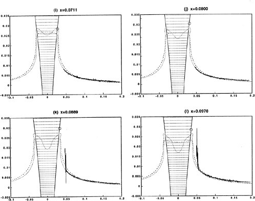
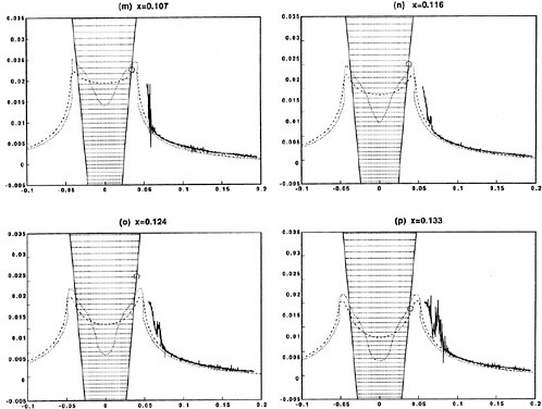

Numerical Simulation of Ship Flow by a Method of Artificial Compressibility
F.Bet, D.Hänel, S.Sharma (Gerhard-Mercator-Universität Duisburg, Germany)
Abstract
A method of solution for the three-dimensional Euler and Navier-Stokes equations is under development for the prediction of flow around ships in restricted water.
The algorithm is based on the concept of artificial compressibility, from which a Roe-like difference splitting scheme for the inviscid fluxes is derived. Free surfaces are tracked by a level-set method. The computations are performed on block-structured grids employing an explicit Runge-Kutta time stepping algorithm.
1 Introduction
A task of major concern in the field of ship hydrodynamics is the accurate calculation of the drag forces of a ship and its characteristic features of propulsion, to make obligatory predictions of these characteristics in the state of project. Due to the high complexity of the real flow around a ship’s body and due to the interaction of the ship and the moving water surface one still depends on small-scale experiments in water channels. Maintaining the Froude-similarity in experimental setups leads generally to a violation of the Reynolds-similarity. Thus the experimental results are generally not similar. The traditional decomposition of the total drag into two independent parts due to waves and friction is physically inadequate due to the correlations between waves and the viscous flow around the ship. In addition, the empirical correction of friction in shallow water commonly used is too inaccurate to transfer solution from the model to the real-scale prototype.
The present work intends to overcome the weaknesses of small-scale experiments (high costs, time consuming, influence of scale) by the determination of a most possible commonly valid theoretical solution using means of modern computational fluid dynamics (CFD).
Our interest is directed to the development of efficient and accurate algorithms for the incompressible Navier-Stokes equations with applications to flow around ships in restricted waters. The algorithmic development is based on previous experiences with the artificial compressibility concept [1] and on multigrid acceleration [2]. The numerical formulation of free surfaces influences remarkably the accuracy and efficiency of the computation. Several attempts exist; a review about them is given by e.g. Mijata [3].
2 Method of Solution
The governing equations are the Navier-Stokes equations for an incompressible fluid influenced by gravity. Normalised by the length of the body L, the undisturbed flow velocity U, the fluid density ρ, and viscosity ν, these equations can be written in the following form:
(1)
(2)
(3)
(4)
with ![]() denoting the total pressure, which consists of a static part (ps) and a geodetic part, both normalised with ρ · U2
denoting the total pressure, which consists of a static part (ps) and a geodetic part, both normalised with ρ · U2
(5)
where y is the coordinate in direction of gravity. The Froude number based to the reference value is ![]() , and the corresponding Reynolds number is Re=UL/ν where ν represents the kinematic
, and the corresponding Reynolds number is Re=UL/ν where ν represents the kinematic
viscosity of water.
The viscous terms σ are defined as follows:
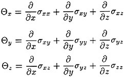
with:
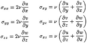
The final equations are transformed to general coordinates, sketched in figure 1:
τ=t, ξ(x, y, z), η(x, y, z), ζ(x, y, z)
and discretized by a finite-volume method in a node-centred arrangement on block-structured curvilinear meshes.
The transformed equations can be written as:
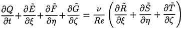
(6)
where:
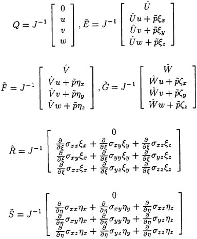
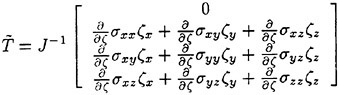
and:
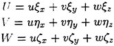
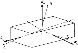
Figure 1: Discrete Control Volume and Coordinate System
The metric factors are defined as:
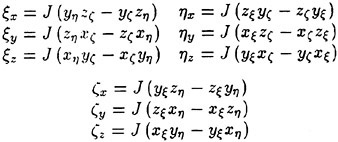
and the Jacobian:
2.1 Concept of Artificial Compressibility
The pressure in a rigourous incompressible flow acts like a relaxation parameter to satisfy the continuity equation ![]() .
.
A possible way to determine the pressure field is the coupling of mass and momentum equations by the concept of artificial compressibility in analogy of compressible flow [4]. This concept is adopted here, based on previous computations in [5] for steady and unsteady incompressible flows.
The original continuity equation (1) is modified by adding an artificial time derivative of pressure representing (artificial) compressibility:
(7)
where β represents a parameter of compressibility. Equation (7) can be deduced from the continuity equation for compressible fluids, by using the equation of state:
(8)
The modified inviscid system of partial differential equations reads now:
(9)
with:
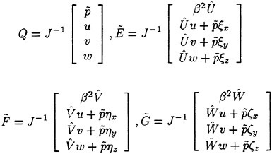
The system is of hyperbolic type, in analogy to the compressible case. Its eigenvalues in the ξ−t plane are e.g.:
(10)
The value of c is given by:
(11)
A comparison with the eigenvalue of the Euler equations for a compressible fluid shows that c corresponds to an artificial speed of sound.
In analogy to the compressible case, an artificial Mach-number can be defined by the relation of the flow velocity to the artificial speed of sound:
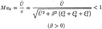
(12)
Small disturbances in pressure propagate in an incompressible fluid with infinite velocity. The artificial compressibility limits the propagation speed. In contrast to an incompressible fluid, the effect of disturbance are delayed. The degree of delay depends on the value of β. For β>0 the pseudo-compressible flow is comparable to subsonic flows.
The solution of the system with modified continuity equation is unphysical for transient flows. At steady-state, however, the time-derivative ![]() is zero and thus the original continuity equation for incompressible fluids is regenerated.
is zero and thus the original continuity equation for incompressible fluids is regenerated.
The propagation speed of a pressure wave in a pseudo-compressible flow is influenced considerably by the selection of the parameter β. An increase of the parameter β results in a disturbance spreading faster into the zone of flow, and the solution will approach more closely to the solution of a completely incompressible flow.
Thus the selection of a suitable value for β is subject to certain restrictions. An upper boundary can be calculated from the relation K between the maximum and the minimum eigenvalue of the differential equation system:
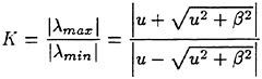
(13)
A higher value for K means a stiff differential equation system with difficult solution.
In the literature different models exist, with the value of β being assumed proportionally to the local flow velocity [6], [7]:
(14)
where the parameter γ is a factor of the order of magnitude 1.
The value for β, received from equation (14), is locally variable. This can lead to difficulties in convergence since the flow rate can become locally very large and thus the parameter β also increases.
A reasonable lower boundary for β can be estimated from the condition that artificial pressure waves propagate faster than the viscous effects.
Altogether small values of β lead to divergence of the solution procedure. For flows examined in the context of this work, values for β between 0.4 and 2.0, dependent on the flow problem, have been proved to be suitable. Figure 2 shows the convergence behaviour of a two dimensional laminar boundary layer flow at different values of the parameter β.
2.2 Numerical Flux Discretisation
The similarity of the system of modified equations (9) with a system for subsonic flow enables the construction of numerical fluxes corresponding to well proved shock-capturing schemes. Therefore several upwind formulations for the artificial compressibility concept were derived and tested in previous studies, like AUSM splitting, flux-vector splitting or Roe splitting. Among them, Roe’s flux-difference-splitting has
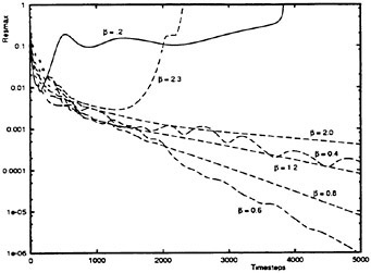
Figure 2: Comparison of the convergence behaviour of the solution procedure at differently values of the parameter β
found to be well suited to achieve close coupling between continuity and momentum equations, necessary for good convergence. The splitting of fluxes is derived from a diagonal transformation of the Jacobian matrix ![]() for example
for example
and by splitting of the eigenvalue matrix:
in Λ=Λ++Λ− with ![]() .
.
From that the numerical flux at a cell interface ![]() and similar expressions in the other directions are given by
and similar expressions in the other directions are given by
(15)
where |A|=R · |Λ| · R−1 is the Roe-matrix and Q± are interface values updated by a second order accurate MUSCL extrapolation. The definition of |A| is numerically evaluated by the computer algebra program MAPLE.
2.3 Treatment of Free Surface
The free surface corresponds to the phase boundary between fluid (water) and gas (air). This boundary is moved according to the flow velocity ![]() .
.
The free surface can be defined by isolines of a function ψ(x, y, z, t)=ψ0=0. The total differential of this function yields the transport equation for the position of the surface, which satisfies the kinematic condition of the surface:
(16)
The dynamic condition describes the continuity of stress across the phase boundary. Neglecting the viscous terms at the surface and the surface tension the dynamic condition reduces to the condition of constant pressure normal to the interphase
where pa is the atmospheric pressure. The boundary condition of the total pressure reads now:
(17)
The combination of equation (16) with system (6) leads to a system of equations similar to equation (6) but completes by one additionally equation for ψ:
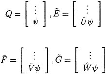
The additional equation for ψ does not change the eigenvalues λ1…4 (10) of the system, but it results in the auxiliary eigenvalue λ5=Û.
The function ψ(x, y, z) divides the integrational domain into three sections as shown in Fig. 3.
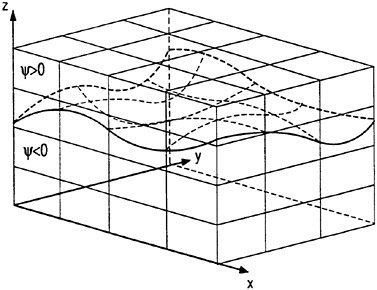
Figure 3: Position of the Free Surface into the Computational Grid
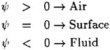
The initial condition for ψ is chosen as:
with yi,j,k and h0 being the distance of each point to the undisturbed free surface and its height, respectively.
The new position of the free surface is calculated by linear interpolation of ψi,j,k after every integration time step.
The flow of air (ψ>0) is presently not of interest, thus the corresponding grid points are used as dummy points to update the boundary conditions in an easy way. Then the dynamic condition given by Eq. (17) is satisfied by an extrapolation of ![]() performed in the way that equation (17) holds on the surface ψ0=0, as sketched in Figure 4. This concept is similar to
performed in the way that equation (17) holds on the surface ψ0=0, as sketched in Figure 4. This concept is similar to
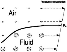
Figure 4: Interpolation Law to Calculate the New Location of the Free Surface
the level-set approach in [8]. The advantages of this approach are:
-
The level set ψ is differentiable over the surface.
-
There is no interruption of the calculations over the surface.
-
Arbitrary surface-inclination up to braking waves are included.
-
Immiscible fluid-fluid interaction can be calculated, (e.g. oil-water).
2.4 Turbulence Model
For turbulent boundary layer computations the laminar viscosity v is replaced by
(18)
where the turbulent viscosity νt is computed by using a standard k−ε model [9]
In this version of the model [10], k and ε are determined from the following pair of equations:
(19)
(20)
The production term Ρ and the two additional source terms D and E are given by the expressions:
(21)
(22)
(23)
The turbulent viscosity is given by:
(24)
and the closure functions are:
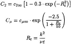
with the constant coefficients:
|
C1 |
c2∞ |
cμ∞ |
σk |
σε |
|
1.44 |
1.92 |
0.09 |
1.0 |
1.3 |
Because of the source terms, the implementation of the turbulence model is accompanied by an additional time scaling. In order to avoid a destabilisation of the calculation by the source terms of the turbulence model, equations (19) and (20) are splitted into a convective-diffusive and a dissipative-productive part:
(25)
(26)
with the vector of turbulent transport properties
the convective-diffusive part
(27)
and the dissipative part:
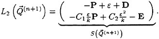
(28)
Equation (25) now is an equation of transport only and can be solved by a standard upwind method. Equation (26) now contains all source terms. Equation (26) are solved implicitly in order to obtain a more stable behaviour of the solution. The source term S is developed into a Taylor series around ![]() :
:
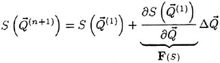
(29)
By introducing (29) into equation (28) and into equation (26) one obtains:
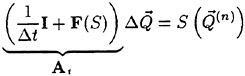
(30)
where I is the matrix of unity. Inverting matrix At leads to:
(31)
with ![]()
2.5 Boundary Conditions
Figure 5 shows the reference frame and ship location. The x direction is positive in the backward facing direction, y is positive upwards, above the free surface and z is positive towards the starboard side. The free stream velocity vector is parallel to the x-axis and points in the same direction. The ship-hull perturbs the uniform flow and is held fixed in place, i.e. the ship is not allowed to translate in y direction or to rotate in the x–z plane. The integrational do
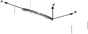
Figure 5: Reference Frame and Ship Location
main is bounded by different types of boundaries as they are free surfaces, walls, inflow/outflow boundaries and symmetry planes.
The treatment of free surface is discussed in a previous section.
Walls are defined by a zero velocity in normal direction.
In viscous flow all velocity components are set to zero according to Stokes no-slip condition.
ur=0, νr=0, wr=0
Values of pressure at a wall have to be deducted from compatibility conditions. For walls with high Reynolds numbers Re the pressure gradient can be neglected because of the boundary layer character of the flow near to the wall, so that on the boundary the pressure can be extrapolated from the flow field with:
At inviscid flows over curved walls e.g. in [11] and [12], the pressure gradient at the wall is not zero. In this case the wall pressure is updated by extrapolation from the interior.
At inflow and outflow boundaries the effect of friction is neglected. Then boundary conditions can be derived from the characteristic solution ![]() of the corresponding Euler equations, with:
of the corresponding Euler equations, with:
where xn is the coordinate normal to the boundary and λ is the eigenvalue in that direction.
The boundary conditions at the inflow edge (index r) are determined by the formulation of the variables ![]() with the inflow conditions (index ∞) and by compatibility conditions (index e), which are determined by extrapolation from the field.
with the inflow conditions (index ∞) and by compatibility conditions (index e), which are determined by extrapolation from the field.
For the inflow boundary follows
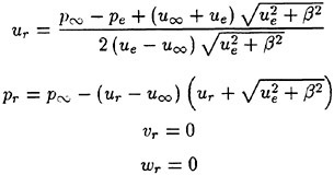
For outflow boundaries, the boundary condition for the pressure is determined by a non-reflecting condition. This permits a disturbance wave to pass a boundary without being reflected and so it does not influence the solution downstream [13]:
(32)
where ![]() is the velocity component normal to the boundary. The square root term
is the velocity component normal to the boundary. The square root term ![]() represents the artificial speed of sound at the boundary and α is an iteration parameter with the value 0.1÷0.2. All other variables at the outflow are extrapolated.
represents the artificial speed of sound at the boundary and α is an iteration parameter with the value 0.1÷0.2. All other variables at the outflow are extrapolated.
A further limitation of the integration domain is the symmetry plane.
From the symmetry condition it follows that the normal gradient of all variables must disappear. Only the velocity component normal to the symmetry plane has to vanish completely ![]() .
.
The transport equations of the turbulence model (19) and (20) need suitable boundary conditions. As for the other flow values, k and ε are given or extrapolated. In this work the following boundary conditions for k and ε are used:
|
inflow bound: |
kr=kmin |
εr=εmin |
|
outflow bound: |
kr=ke |
εr=εe |
|
symmetries bound: |
|
|
|
fixed wall: |
kr=0 |
εr=0 |
where the indices r and e representing the boundary and the extrapolated values, respectively. The values kmin and εmin result from the largest values for k and ε in the field:
kmin=kmax · 10−5 εmin=εmax · 10−5
2.6 Integration in Time
Equation (6) is integrated in the time by an explicit multistage scheme. Hence equation (9) can be written in a semi-discrete form:
(33)
where Res(Q) is the discrete space approach of equation (9) The multistage time stepping scheme is formulated as:
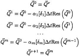
The coefficients (αn) are chosen to maximise the stability of the system and the optional coefficients (δn) is employed in the equation for ψ to allow an individual optimisation towards best stability.
A five stage-scheme with three evaluations of the level-set equation has been found to be particularly effective. Its coefficient are:
|
α1=1/4 |
δ1=0 |
|
α2=1/6 |
δ2=0 |
|
α3=3/8 |
δ3=1 |
|
α4=1/2 |
δ4=1 |
|
α5=1 |
δ5=1 |
3 Computational Results
A number of calculations of viscous and inviscid flow, mainly in 2-D, were performed to validate the present solution concept and the treatment of free surfaces [11].
In the following, two classical 3-D examples are presented which enable the comparison with other results, in particular for the wave pattern. To enable direct comparisons with inviscid computations in [6] and to eliminate effects of insufficient turbulence modelling, the following calculations are performed likewise for inviscid flow.
The flow past the wigley hull and the serie-60 ship are presented here as computational examples, since for both configuration many numerical and experimental results are available [6] [14].
The Figures 6 and 7 show portions of the generated
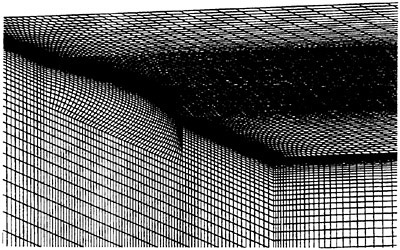
Figure 6: Calculations Grid for Wigley Hull Computation
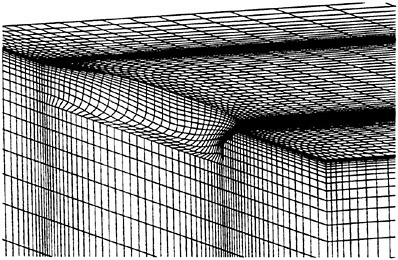
Figure 7: Calculations Grid for Serie-60 Hull Computation
grids. The grid points are clustered near the bow and stern in the x-direction, near the free surface in the
y-direction and near the ship hull in the z-direction. The grid extends a half ship length upstream from the bow, ![]() ship lengths downstream from the stern,
ship lengths downstream from the stern, ![]() ship lengths to starboard and 1 ship length down below the undisturbed free surface. Figure 8 shows the wave patterns along the wigley hull model at a Froude number Fn=0.250 (top) and along the serie-60 model at a Froude number Fn=0.326 (bottom). The waterline contours, compared with experimental
ship lengths to starboard and 1 ship length down below the undisturbed free surface. Figure 8 shows the wave patterns along the wigley hull model at a Froude number Fn=0.250 (top) and along the serie-60 model at a Froude number Fn=0.326 (bottom). The waterline contours, compared with experimental
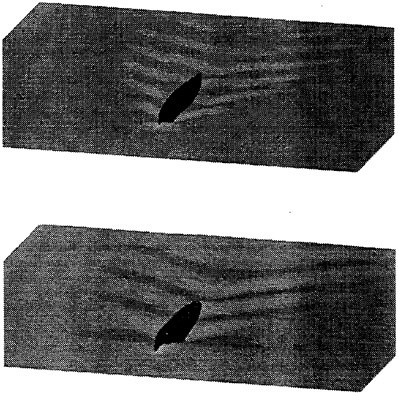
Figure 8: Wave Patterns for Wigley-Hull Model at Fn=0.250 (Top) and for Serie-60 Model at Fn=0.316 (Bottom) (Wave Heights are 3 times magnified)
results [15] are shown at Figure 9. The computed
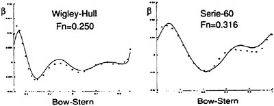
Figure 9: Computed vs. Experimental Wave Elevation
wave drag coefficient in Fig. 10, obtained by integrating the longitudinal component of pressure on the wetted hull surface, show sufficiently well agreement with the experimentally determined values of the wave drag coefficient, Cw(exp)=0.821 · 10−3 for the wigley hull and Cw(exp)=2.6 · 10−3 for the serie-60 model.
The overhead wave profiles, computed for both ship
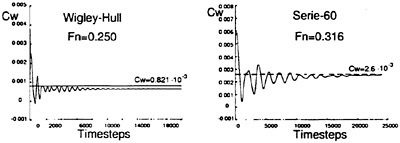
Figure 10: Computed vs. Experimental Wave Drag
configurations, are presented in Figure 11. The simu
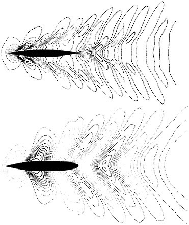
Figure 11: Computed Overhead Wave Profiles, Wigley-Hull, Fn=0.250 (top), Serie-60, Fn=0.316 (bottom)
lation of viscous flow with free surface is of particular interest. In order to validate the model calculations with and without free surface have been performed. An example of a viscous flow with free surface is represented in figure 12. There the deformation of a free water surface, which is due to the formation of a boundary layer in the flow at a flat partly immersed plate, is shown. The friction coefficient cf is given at different water levels in figure 13. The difference relative to the theoretical (Blasius) value is very small at large distance from the free water surface, only near to the free surface the values differ considerably. This difference is a consequence of the interaction of the
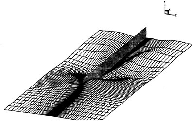
Figure 12: Boundary layer and wave Patterns for a flat plate at Re=1000. (Wave Heights are 3 times magnified)
free surface with the boundary layer. In order to val
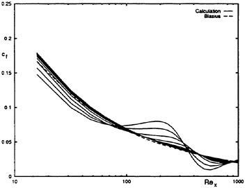
Figure 13: cf vs. Rex comparison between calculation and theory (Blasius)
idate the turbulence model a two-dimensional flow around a plate has been taken. The computational domain reaches from x=−.5 L to x=1 L where L is the length of the plate. The upper boundary of the computational domain is about 2δ where δ represents the thickness of the boundary layer. Figure 14 shows the local friction coefficient cf at a Reynolds number Re=5 · 106. In figure 15 the velocity profile and the distribution of turbulent viscosity above the plate at x/L=0.9 is printed.
Figure 16 contains the distribution profile of k and ε again on the upper side of the plate at x/L=0.9.
Further calculations of three dimensional problems, especially viscous turbulent flows around ships, are actually performed and will be presented at the conference.
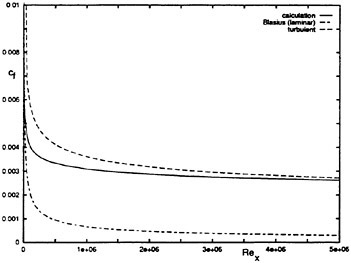
Figure 14: Local resistance for flat plate at zero incident (Re=5 · 106); comparison between calculation and theory
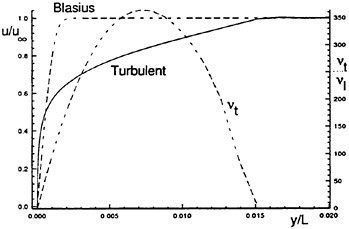
Figure 15: Turbulent and laminar velocity profile and turbulent viscosity profile over the plate at x/L=0.9
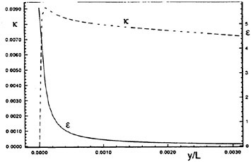
Figure 16: Profile of the turbulent kinetic energies k and dissipation rate ε over the plate at x/L=0.9
References
[1] D.Hänel, M.Breuer, J.Klöker, M.Meinke: Computation of Unsteady Vortical Flows. Computer & Fluids, vol. 22, pp. 229–237, 1993.
[2] D.Hänel, M.Meinke, W.Schröder: Multigrid Solutions for the Navier-Stokes Equations. In: E.H.Hirschel (Editor): Finite Approximations in Fluid Mechanics II. Notes on Num. Fluid Mechanics, vol 25, pp. 176–190, Vieweg Verlag Braunschweig, 1989.
[3] H.Miyata. Free-Surface Flow Simulations by Finite Difference Techniques. Computational Fluid Dynamics 94, 1994.
[4] A.J.Chorin. A Numerical Method for Solving Incompressible Viscous Flow Problems. Journal of Computational Physics, 2:12–26, 1967.
[5] M.Breuer. Numerische Lösung der Navier-Stokes-Gleichungen für dreidimensionale inkompressible instationäre Strömungen zur Simulation des Wirbelaufplatzens. PhD thesis, RWTH Aachen, 1991.
[6] J.Farmer, L.Martinelli, and A.Jameson. A Fast Multigrid Method for Solving the Nonlinear Ship Wave Problem with a free surface. In 6th International Conference on Numerical Ship Hydrodynamics. Iowa City, Iowa, 2–5 August 1993.
[7] T.Hino, L.Martinelli, and A.Jameson. A Finite-Volume Method with Unstructured Grid for Free Surface Flow Simulations. Sixth International Conference on Numerical Ship Hydrodynamics, 1993.
[8] M.Sussman, P.Smereka, and S.Osher. A Level Set Approach for Computing Solutions to Incompressible two-Phase Flow. Journal of Computational Physics, 114:146–159, 1994.
[9] B.E.Launder and D.B.Spalding. The Numerical Computation of Turbulent Flows. Computer Methods in Applied Mechanics and Engineering, 3:269–289, 1974.
[10] Virendra C.Patel, Wolfgang Rodi, and Georg Scheuerer. Turbulence Models for Near-Wall and Low Reynolds Number Flows: A review. AIAA, 23(9):1308, September 1985.
[11] F.Bet, D.Hänel, and S.D.Sharma. Simulation of Hydrodynamical Free-Surface Flow. In Proc. of Eccomas 96. INRIA, Paris, John Wiley & Sons, Ltd., 1996.
[12] F.Bet, D.Hänel, and S.D.Sharma. Simulation of Ship Flow. In Proc. of Numerical Methods in Laminar and Turbulent Flow. 10th International Conference, Swansea 1997, Pineridge Press Limited, 1997.
[13] A.Jameson, W.Schmidt, and E.Turkel. Numerical Solutions of the Euler Equations by Finite Volume Methods using Runge-Kutta Time-Stepping Schemes. In Proc. of AIAA 14th Fluid and Plasma Dynamics Conference. AIAA, Palo Alto, California, 1981.
[14] H.Miyata, M.Zhu, and O.Watanabe. Numerical Study on a Viscous Flow with Free-Surface Waves about a Ship in Steady Straight Course by a Finite Volume Method. Journal of Ship Research, 36:332–345, 1992.
[15] Y.Toda, F.Stern, and J.Longo. Mean Flow Measurements in the Boundary Layer and Wake and Wave Field of a serie 60 cb=0.6 Ship Model for Froude Numbers .16 and .316. Technical Report 352, Iowa Institute of Hydraulic Research, The University of Iowa, 1991.
[16] M.Meinke and D.Hänel. Time Accurate Multigrid Solutions of the Navier-Stokes Equation. In Proc. of Third European Conference on Multigrid Methods, Oct 1990.
Unsteady RANS CFD Method for Naval Combatants in Waves
R.Wilson, E.Paterson, F.Stern (University of Iowa, USA)
ABSTRACT
This paper documents the development of CFDSHIP-IOWA version 3.0. This work has been motivated by the accuracy and efficiency requirements for simulating naval combatants maneuvering in waves. Version 3.0 is based upon extensions of version 2.1 which is a general-purpose parallel-multiblock RANS code using finite analytic discretization and the PISO algorithm. The new core solver is based upon higher-order upwind finite differences. Two methods for pressure-velocity coupling were explored—a projection method and pressure-implicit split operator (PISO) method. Steady flow verification and validation is presented for the code-development benchmark geometries which includes the Wigley hull, Series 60 CB=0.6 and DTMB Model 5415. Unsteady flow results are presented for the Wigley hull and DTMB Model 5415. For the former, comparisons are made to Rhee and Stern (1998). For the latter, preliminary results using version 2.1 are presented.
The overall structure of CFDSHIP-IOWA, which was designed for generality, modularity, and MPI-based parallel multiblock, provides a framework for code development and high-performance computing. Implementation for version 3.0 is straightforward. The method shows significant improvement in comparison to version 2.1, as demonstrated through reduced uncertainties and qualitative comparisons, for both accuracy and efficiency. Results show that the use of PISO for the pressure-velocity coupling greatly improves robustness and stability and that its use is required to obtain solutions for complex geometries where grids were highly skewed. The unsteady results for the Wigley hull show much promise for version 3.0 in that it compares very well to the validated solutions of Rhee and Stern (1998). Moreover, due to higher-order discretization of the KFSBC solver, the diffraction wave pattern for version 3.0 solution shows improved results and less dissipation.
1 INTRODUCTION
The flow around a surface ship in the open ocean environment is extremely complicated due to not only the ship’s geometry and associated turbulent boundary layers, wakes, and wave fields, but the ambient wind and waves, motions, and maneuvering. Although both design methods and physical understanding are based upon the historical approach of decomposing the problem into resistance and propulsion, seakeeping, and maneuvering, each of which uses a variety of experimental, computational and empirical methods, recent advances in Reynolds-averaged Navier-Stokes (RANS) CFD give hope of developing simulation-based design tools which incorporate environmental effects. The capability for such simulations does not yet exist due to limitations in both computer resources and phenomenological models. Nevertheless, the objectives of the work herein represents a first step by incorporating an incident wave field into the unsteady RANS simulation of a naval combatant (Figure 1).
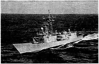
Figure 1. Naval Combatant in Waves. (US Navy Photo)
Even this simplified problem contains a wide range of physics and scales to resolve including high Reynolds number unsteady boundary layers and wakes, a liquid-air free-surface with breaking waves,
spray, and bubble generation, and, in the case of a modern naval combatant at cruise speed, a naturally unsteady flooded-transom wake. The latter of which may interact with the forced unsteadiness of the incident wave field. Moreover, there are a variety of other important effects which must be modeled including turbulence anisotropy and interaction with the free surface, bubbly flow, thermal and density stratification, and surface tension and surfactants. Physical understanding of these phenomenon are critical in developing new models, predicting performance and hydrodynamic signatures, and developing counter weapons and measures.
RANS methods have seen increasingly broad application to many of the challenges in ship hydrodynamics. As recent as 1994, the CFD Workshop Tokyo (1994) was organized to assess the status of steady RANS methods for solution of free-surface flows around surface ships. Since then, for example, RANS methods have been used and further developed for simulation of two-phase bubbly and stratified flows around naval combatants (Paterson et al., 1996), maneuvering submarines with rotating propellers (McDonald and Whitfield, 1996), and, most recently, surface ships in head waves (Rhee and Stern, 1998). Rhee and Stern (1998) will subsequently be referred to as R&S.
At the Iowa Institute of Hydraulic Research (IIHR), a general purpose CFD code, CFDSHIP-IOWA, has been developed for general application, research, and transition. It is an unsteady incompressible RANS code which has been transitioned to the science and technology, research and development, and design, test, and evaluation communities. It has its origin in the work of Tahara and Stern (1996) but has been extensively rewritten to address the issues of modularity, generality, and scalable parallel computing (Paterson et al., 1998). It has capability for nonlinear free-surface flows, moving grids, and linear and non-linear turbulence closures. The currently released version (i.e., v2.1) is based upon finite-analytic discretization and the PISO algorithm. Distribution of source code, documentation, and examples is accomplished via a WWW site (http//www.iihr.uiowa.edu/~cfdship/)
Although v2.1 of CFDSHIP-IOWA has well documented performance for steady-flow simulation of naval combatant geometries (e.g., Stern et al., 1996; Paterson et al., 1998), improved accuracy and efficiency is required to simulate Challenge-scale problems such as a combatant maneuvering through waves. This has provided the motivation for the work of R&S and the development of version 3.0 (v3.0) of CFDSHIP-IOWA.
R&S has presented unsteady RANS CFD simulations for the Wigley hull in head waves for a range of conditions (i.e., Froude number, wave steepness, and wave amplitude) including detailed verification and validation. As such, this work has provided much guidance to the CFD code development efforts at IIHR. A generalized version of the R&S unsteady RANS algorithm has been compared to a PISO approach in v3.0 of CFDSHIP-IOWA.
The objectives of the current study are verification and validation of v3.0 of CFDSHIP-IOWA for unsteady flow of a fixed steadily-advancing naval combatant in regular head waves. The approach is based upon a series of validation geometries which include the Wigley hull, Series 60 CB=0.6, and DTMB Model 5415. Calm sea (i.e., steady flow) results will also be presented for verification and validation purposes.
The paper is organized as follows. In Section 2, governing equations, boundary and initial conditions, and numerical method and solution procedure are presented. Then, in Section 3, model problems, conditions, and grids are described along with available validation data. In Section 4, uncertainty assessment is performed and presented. Section 5 presents discussion of both steady and unsteady results for the model problems and, finally, Section 6 provides conclusions and future work.
2 CFDSHIP-IOWA—VERSION 3.0
In this section, the numerical method is described. Governing equations are presented in Section 2.1 followed by boundary and initial conditions in Section 2.2. The numerical method for solution of the RANS equations and kinematic free-surface boundary conditions in v3.0 are presented in Section 2.3. Detailed description of the numerical method for v2.1 is given in Paterson et al. (1998).
2.1 Governing Equations
In non-dimensional and Cartesian tensor notation form, the unsteady incompressible RANS and continuity equations are written as
(1)
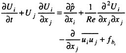
(2)
where Ui=(U, V, W) are the mean-velocity components, xi=(Χ, Υ, Ζ) are the Cartesian
coordinates, ![]() is the piezometric pressure (p+Z/Fr2),
is the piezometric pressure (p+Z/Fr2), ![]() are the Reynolds stresses, ν is the kinematic viscosity,
are the Reynolds stresses, ν is the kinematic viscosity, ![]() are the body-force terms, which represent the effects of the propeller,
are the body-force terms, which represent the effects of the propeller, ![]() is the Froude number, and Re=UoL/ν is the Reynolds number. The Reynolds stresses are related to the mean rate of strain through an isotropic eddy viscosity νt
is the Froude number, and Re=UoL/ν is the Reynolds number. The Reynolds stresses are related to the mean rate of strain through an isotropic eddy viscosity νt
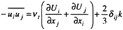
(3)
where δij is the Kronecker delta and k is the turbulent kinetic energy. The equations are normalized by reference velocity Uo, length L, and density ρ.
Substituting (3) for the Reynolds-stress term in (2), the momentum equations become
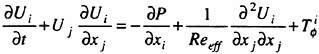
(4)
where:
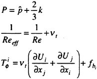
Eddy viscosity is calculated using one of three models: Baldwin-Lomax; Menter’s blended k-ω/k-ε; or Chen and Patel 2-layer k-ε. For the Baldwin Lomax model, eddy viscosity is calculated for each no-slip surface in the domain and then a weighted averaged computed based upon the wall distance y+ to each surface. For the blended k-ω/k-ε model, three options are available: standard model; a shear-stress transport model, and a low-Re model. For the two-layer k-ε model, matching between layers is fixed at a y+=150 and the near-wall model is turned off in the wake.
The equations are transformed from the physical domain in Cartesian coordinates (x, y, z, t) into the computational domain in non-orthogonal curvilinear coordinates (ξ, η, ζ, τ). A partial transformation is used in which only the independent variables are transformed, leaving the velocity components Ui in Cartesian coordinates. Details of the coordinate transformation can be found in Stern et al. (1996). The continuity (1) and momentum (2) equations in the transformed space are given by
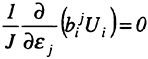
(5)
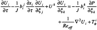
(6)
where ![]() are the metrics of the transformation, J is the Jacobian, and
are the metrics of the transformation, J is the Jacobian, and ![]() is the contravariant velocity component.
is the contravariant velocity component.
2.2 Boundary and Initial Conditions
Twenty different boundary condition types can be specified in the input to CFDSHIP-IOWA. They can be organized into physical (i.e., no-slip, free surface, traveling-wave inflow), computational (i.e., uniform inflow, exit, far-field, zero-gradient, symmetric, periodic, cut, pole, impermeable zero stress) and multi-block (i.e., patched and overset) conditions. Most of these are self explanatory or have been documented elsewhere (e.g., Stern et al., 1996; Paterson et al., 1998). Therefore, for brevity, only the free-surface and traveling-wave inflow will be further discussed.
The free surface boundary conditions are based upon the exact nonlinear kinematic and approximate dynamic free-surface boundary conditions, both of which are applied on the actual free surface. The kinematic equation is a 2D hyperbolic wave equation for the wave elevation ζ
(7)
The dynamic condition requires that stress across the free surface is constant. The three components of stress provide boundary conditions for U, V, and Ρ and are derived by neglecting external stress and surface tension and by assuming small curvature and small gradients of normal velocity. A boundary condition for W is derived from the continuity equation, i.e., Wz=−Ux−Vy.
The incident wave field is imposed on the inlet boundary and modeled as velocity and pressure perturbations which are added to the uniform stream. It is derived from the linear potential flow solution for a free-surface traveling wave (e.g., Newman, 1977)
(8)
(9)
(10)
(11)
(12)
where ω, ωe, A, k, and λ are the traveling wave frequency, incident frequency, amplitude, wave number, and wavelength, respectively.
Three initial conditions are available in CFDSHIP-IOWA: uniform free-stream, start from rest, and restart from either a previous solution or user-generated data set. For the start-from-rest condition, the forward speed of the ship is smoothly accelerated to unity through the use of a hyperbolic tangent function for U0(t). For the unsteady simulation of a ship in waves, only the long-time periodic response is of current interest. Therefore, to reduce the initial transients, the perturbations in Eqn. (8)–(12) are added to the converged steady state solution and used as the initial condition.
2.3 Numerical Method
The continuous momentum equation Eqn. (6) is reduced to algebraic form through the use of finite-differences. The-continuity equation is enforced through a pressure-based method where a pressure-Poisson type equation is derived. Details of the numerical method are given in the next three sections.
2.3.1 Discretization
For temporal discretization, a general formula for an Euler backward difference is given by
(13)
where the weights, wt, determine the order of the difference expression and are given in Table 1 for the first- and second-order formulations. For steady state solutions, the first-order formulation is used while the second-order formulation is used for the time-accurate solution procedure.
Table 1. Finite-difference weights for temporal discretization.
|
Scheme |
wtn |
wtm |
wtmm |
|
First-order |
1 |
−1 |
0 |
|
Second-order |
3/2 |
−2 |
1/2 |
For spatial discretization, the convective terms are discretized with the following higher-order upwind formula
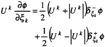
(14)
where:
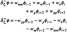
Six convective schemes are available in CFDSHIP-IOWA and their coefficients are supplied in Table 2. For the computations presented here, the third-order upwind scheme is used.
Table 2. Finite-difference weights for spatial discretization of convective terms.
|
Scheme |
wmm |
wm |
wn |
wp |
wpp |
|
1st order upwind |
0 |
−1 |
1 |
0 |
0 |
|
2nd order central |
0 |
-1/2 |
0 |
1/2 |
0 |
|
2nd order upwind |
1/2 |
−2 |
3/2 |
0 |
0 |
|
Quick |
1/8 |
−7/8 |
3/8 |
3/8 |
0 |
|
3rd order upwind |
1/6 |
−1 |
1/2 |
1/3 |
0 |
|
4th order central |
1/12 |
−2/3 |
0 |
2/3 |
1/12 |
All other first-derivative and viscous terms are discretized using standard second-order central differencing.
Applying the temporal and spatial discretizations given by Eqns. (13) and (14) to the continuous momentum equations (6) gives
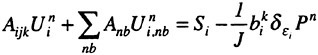
(15)
where Aijk and Anb denotes the central and neighboring coefficients of the discretized momentum equations, respectively. The source term, Si, contains the velocity at the previous time step and the mixed derivative terms originating from the viscous terms which are lagged to the previous iteration.
2.3.2 Pressure-Velocity Coupling
For the pressure-velocity coupling and enforcement of the continuity equation, two approachs were investigated; (i) the projection method and (ii) the PISO method. Issues related to stability and robustness of the two methods will be discussed in Section 5. The two methods are summarized below.
2.3.2.1 Projection Method
A two step procedure is used two enforce the continuity equation for the projection method. In the first step, a pressure-Poisson equations is solved were the velocities in the source term are lagged at the previous iteration. The momentum equations are advanced in time using the computed pressure in the second step. Because an implicit scheme is used for the momentum equations and the velocities in the source term of the Poisson equation are lagged, iteration is required to satisfy both the continuity and momentum equations at each time step.
The pressure equation is derived by taking the divergence of Eqn. (15) and by projecting the velocity into a divergence-free field at time level (n). The result is
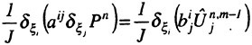
(16)
where aij=Jgij and ![]() . Subscript m-l is used to denote a quantity at the current time level but previous iteration. Use of the standard second-order operator,
. Subscript m-l is used to denote a quantity at the current time level but previous iteration. Use of the standard second-order operator, ![]() in Eqn (16) leads to an odd-even grid point decoupling. To prevent oscillations, fourth-order dissipation is added following Sotiropoulos and Abdallah (1992) by taking a linear combination of full- and half-cell operators:
in Eqn (16) leads to an odd-even grid point decoupling. To prevent oscillations, fourth-order dissipation is added following Sotiropoulos and Abdallah (1992) by taking a linear combination of full- and half-cell operators:
(17)
where L, ![]() N, and S are defined as:
N, and S are defined as:
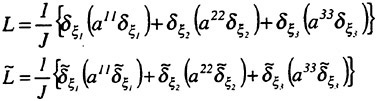
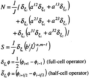
where γ is the weighting value between the full- and half cell formulations. For the computations presented here γ=0.1 is used. Use of the half-cell operator introduces metrics at half-cell locations which are computed from an average of the nodal values.
2.3.2.2 PISO Method
The PISO method uses a predictor-corrector approach to advance the momentum equation while enforcing the continuity equation. The momentum equation (15) is advanced implicitly using a guessed pressure field, P0 in the predictor step:
(18)
where superscript ‘*’ is used to denote advancement to an intermediate time level.
In the corrector step, the pressure-Poisson equation is solved and then the velocity is explicitly updated by the following equations:
(19)
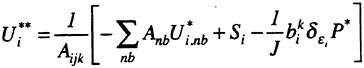
(20)
where L, ![]() N, and S are defined in Eqn. (17) with a modification to the geometric coefficients, aij=Jgij/Aijk. Equations (19) and (20) can be repeated in a loop for additional corrector steps.
N, and S are defined in Eqn. (17) with a modification to the geometric coefficients, aij=Jgij/Aijk. Equations (19) and (20) can be repeated in a loop for additional corrector steps.
2.3.3 Kinematic Free-Surface Boundary Condition
The kinematic free-surface boundary condition eqn. (7) is discretized using (13) and (14) and solved on the block faces which correspond to the free surface. Given the solution for ζ, the volume grid for each free-surface block is conformed to the new wave elevation through the use of cubic-spline interpolation in the ζ curvilinear coordinate. For
stability reasons, however, several numerical concerns must be addressed.
First, a combination of highly-clustered near-wall spacing (i.e., 10−6 or less) and lack of either physical or numerical dissipation (i.e., for the higher-order schemes) results in an unstable numerical system. Secondly, the KFSBC becomes singular at the no-slip/free-surface intersection due to the “contact line” problem. At the intersection point, the fluid velocity is zero due to the no-slip condition and at the same time the wave elevation on the hull is in motion: an obvious contradiction.
To address both of these problems, near-wall blanking and solution filtering are used. An approximate contact-line model is implemented wherein the highly-clustered near-wall region is blanked out for solution of ζ. Values of ζ in this region are obtained using linear extrapolation. To maintain stability and eliminate spurious oscillations, ζ is filtered with a variable-order (2nd, 4th, or 6th) filter after each iteration.
The overall solution scheme and velocity-pressure coupling is based upon the projection method. For a given time step, the method is summarized as follows
-
Solve KFSBC and conform grid to wave field.
-
Solve pressure equation.
-
Solve 2-equation turbulence model equations, if applicable, and calculate eddy viscosity.
-
Solve momentum equations with new pressure.
-
Return to (1) until pre-selected convergence criterion met.
-
Post-processing.
-
Next time step.
The method is fully implicit and therefore requires iterative solvers. Currently, a line-ADI scheme with pentadiagonal solvers and under relaxation is used to solve the algebraic equations that arise from discretization of the momentum, pressure Poisson, and KFSBC equations.
3 GEOMETRIES, CONDITIONS, AND GRIDS
In this section, geometries, simulation conditions and EFD validation data, and numerical grids will be described.
Code development efforts at IIHR are guided by the use of standard benchmarks. The surface-piercing flat plate, surface-piercing NACA0024 foil, Wigley hull, Series 60 CB=0.6, and David Taylor Model Basin (DTMB) Model 5415 have been chosen because of applicability and available EFD validation data. Herein, results for the three ship geometries are presented. The Wigley hull and Series 60 are both cruiser sterns whereas the Model 5415 is representative of a modern naval combatant with both a sonar dome and a transom stern.
Simulation conditions are set to the EFD conditions. Available steady flow data includes Journee (1992) for the Wigley hull, Toda et al. (1992) for the Series 60, and Ratcliffe (1998) for DTMB Model 5415. For unsteady flow, very little data is available. Journee (1992) has data for Wigley hull in head waves. It should be noted that, currently, an international collaborative project is underway to build an extensive CFD validation database for Model 5415 (and smaller geomsims). Participants include DTMB, IIHR, and INSEAN in Rome. Each facility will deliver different parts of the database, i.e., propeller-hull interaction, unsteady flow for ship in head waves, and detailed steady-flow mapping, respectively.
Table 3. Conditions for steady flow simulations
|
|
Wigley |
Series 60 |
DTMB 5415 |
|
Re |
4.86×10⁶ |
4.3×10⁶ |
1.39×10⁷ |
|
Fr |
0.30 |
0.316 |
0.28 |
The conditions used in the steady and unsteady flow simulations are defined in Tables 3 and 4, respectively.
Table 4. Conditions for unsteady flow simulations
|
|
Wigley |
DTMB 5415 |
|
Re |
4.86×10⁶ |
1.39×10⁷ |
|
Fr |
0.30 |
0.28 |
|
Ak |
0.052 |
0.026 |
|
Α/λ |
0.0082 |
0.0042 |
Figure 2 shows a typical half-domain grid system. The boundary conditions used include inlet (SI), exit (SE), no-slip (SB), far-field (S0), centerplane symmetry (SCP), patched multiblock (SMB), and free surface (SF).
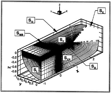
Figure 2. Grid System for Model 5415 with Boundary Condition Types
Body-fitted, structured, multi-block grids are generated using the commercial grid generation code GRIDGEN from Pointwise, Inc. The grids for Wigley hull and Series 60 are single block and use an H-type grid topology with grid clustering near the bow and stern in the ε-direction, at the hull in the η-direction, and near the free surface in the ζ-direction. Near-wall spacing is determined by turbulence modeling considerations where, in general, the first point from the no-slip surface is placed at a normalized wall distance of y+<1.0. For the Wigley hull, no grid studies were performed with v3.0 since, as discussed below, Rhee and Stern (1998) presented detailed grid studies with a similar numerical scheme. The Wigley hull grid has 105×61×30=192,150 points. In contrast, 3 grids, with a refinement ratio ![]() in each coordinate direction, are used for the Series 60. The sizes of the coarse, medium, and fine grids are 144×36×22=114,048, 200×51×30=306,000, and 287×73×43=900,893, respectively.
in each coordinate direction, are used for the Series 60. The sizes of the coarse, medium, and fine grids are 144×36×22=114,048, 200×51×30=306,000, and 287×73×43=900,893, respectively.
For the multi-block Model 5415 calculations, patched multi-block grids and boundary conditions are used. Grid clustering locations are similar to the other hulls however different topology is required especially for the transom. In this case, a separate block is placed in the transom wake. Figure 2 shows the 5-block grid system for Model 5415. It has 3 blocks on the free surface and consists of blocks of size 75×51×21, 75×51×40, 76×51×21, 76×51,40, and 40×51×21. Total system size is 510,561 points. A set of 3 grids for assessing grid uncertainty have not yet been designed for Model 5415.
4 UNCERTAINTY ASSESSMENT
CFD uncertainty assessment consists of documentation, verification, and validation. Documentation is self explanatory but, nevertheless, often not provided. An overview of verification and validation is presented in the following.
Simulation uncertainty is divided into two components, one from numerics USN and the other from modeling USM. The numerical uncertainty in the simulation can be assessed using verification analysis methods (Stern et al., 1996; Stern et al., 1998). Therein, USN is estimated for both point and integral quantities and is based upon grid and parametric studies which determine grid USG, iterative USI, and time-step UST uncertainties. A root sum square (RSS) approach is used to combine the components and to calculate USN.
CFD validation follows the method of Coleman and Stern (1997). Therein, a new approach is developed where uncertainties from both the simulation (i.e., US) and EFD benchmark data (i.e., UD) are considered. The first step is to calculate the comparison error Ε which is defined as the difference between the data D (benchmark) and the simulation prediction value S
(21)
The validation uncertainty UV is defined as the combination of UD and the portion of the uncertainties in the CFD simulation that are due to numerics USN and which can be estimated through verification analysis:
(22)
UV sets the level at which the validation can be achieved. The criterion for validation is that | E | must be less that UV. Note that for an analytical benchmark, UD is zero and UV is equal to USN. Validation is critical for making improvements and/or comparisons of different models since USM is buried in UV. A detailed example of the verification procedure for computation of free-surface flow is provided by R&S.
4.1 Wigley Hull
Steady and unsteady flow results for the Wigley hull are provided in Section 5 along with a comparison between v3.0 and R&S. Verification and validation for the Wigley hull simulation was not performed using v3.0 since detailed uncertainty assessment has already been presented by R&S. A summary of this analysis is provided in Section 5.
4.2 Series 60 CB=0.6
Grid convergence is addressed by performing steady simulations for the Series 60 using three computational grids with refinement, ![]() in each coordinate direction. Ship forces from these simulations are given in Table 5 along with the change, ε, between the medium/coarse and fine/medium grid solutions. The results show that the total, pressure, and frictional resistance (i.e., CT, CP, CF) are grid convergent and that USG, which is the relative change in fine and medium grid values, is equal to 1.4%, 1.2%, and 1.5%, respectively.
in each coordinate direction. Ship forces from these simulations are given in Table 5 along with the change, ε, between the medium/coarse and fine/medium grid solutions. The results show that the total, pressure, and frictional resistance (i.e., CT, CP, CF) are grid convergent and that USG, which is the relative change in fine and medium grid values, is equal to 1.4%, 1.2%, and 1.5%, respectively.
Iterative convergence uncertainty USI is assessed through examination of the iteration record of integral and point quantities and is taken as one-half the range of the quantity of interest once initial transients have died out. This is the preferred metric because USI can be directly evaluated. Although residuals, or change between iterates, are often shown, they are not by themselves helpful in assessing USI. Figure 3 shows
Table 5. Grid convergence of ship forces (×10−3), Series 60, Fr=0.316, Re=3.40×10⁶.
|
Grid |
Coarse 144×36×22 |
Medium 200×51×30 |
Fine 283×71×43 |
|
CT |
5.28 |
5.13 |
5.06 |
|
ε |
|
−2.8% |
−1.4% |
|
CP |
1.75 |
1.70 |
1.68 |
|
ε |
|
−2.9% |
−1.2% |
|
CF |
3.54 |
3.42 |
3.37 |
|
ε |
|
−3.4% |
−1.5% |
Figure 3. Iterative Convergence: Series 60. (a) residuals, (b) resistance
both the residuals and the iteration record for resistance on the coarse grid. Note that for the start-from-rest initial condition, the residuals start out very small, increase, and then decrease to about 10−6 at 2000 iterations. The iteration record for resistance, however, shows that CT, CP, and CF are nearly constant beyond 3000 iterations and that USI is several orders of magnitude less than USG. As such, USI can be assumed zero for this grid. Note, however, that the fine grid after 4000 iterations showed a USI=6.5%.
Since explicit artificial dissipation is not used, i.e., USAD=0, and the simulation is for steady flow, i.e., UST=0, the total numerical uncertainty USN for CT is equal to
4.3 Model 5415
Verification and validation results for steady DTMB 5415 simulation, have not yet been fully completed. A status report for v2.1 simulations is presented and discussed in Paterson et al. (1998).
5 RESULTS
Results from steady state simulations of the Wigley hull, Series 60, and DTMB 5415 are presented in Section 5.1 while results from the Wigley hull in regular head waves are presented in Section 5.2.
As described in Section 2.3, two methods for the pressure/velocity coupling were explored in the v3.0 code. For less complex geometries (i.e. the Wigley hull) and computational grids, both the projection and PISO pressure/velocity coupling methods produced equivalent converged solutions. For more complex geometries like the Series 60 robustness was an issue and modifications to the solution procedure (e.g., initially using a large number of sub-iterations, using initial conditions of stagnant flow) were required to obtain a converged solution with the projection method. Such special treatment was not required to obtain an converged solution using the PISO method. It was found that use of the PISO method was required to obtain converged solutions for the DTMB 5415 geometry where special treatments were not sufficient to obtain converged solutions with the projection method.
In Section 5, unless stated otherwise, results from the v3.0 code are presented for the projection method since at convergence both methods produce equivalent results. Results for the DTMB 5415 geometry presented in Section 5.1 were obtained with the PISO method.
5.1 Steady Flow
Wigley Hull
Results from the steady flow simulation of the Wigley hull using v3.0 are presented in this section and compared to those from R&S. This steady flow condition corresponds to the base case solution from R&S wherein Fr effects were studied for steady flow. Validation was not performed for this geometry since a detailed study using similar numerical methods appears in R&S.
Figure 4 shows the computed wave profile along the ship hull in comparison to R&S. Experimental wave profiles were not measured for this condition.
Table 6. Comparison of forces (×10−3) for steady Wigley hull simulation, Fr=0.3, Re=4.86×10⁶.
|
Force |
D |
Sv3.0 |
SR&S |
E*=Sv3−SR&S |
|E| |
UV |
USN |
|
CT |
5.89 |
5.69 |
5.65 |
0.7% |
1.1% |
3.8% |
2.9% |
|
CP |
N/A |
2.18 |
1.95 |
4.0% |
- |
- |
12.3% |
|
CF |
N/A |
3.53 |
3.70 |
−3.0% |
- |
- |
0.04% |
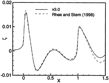
Figure 4. Hull Waterline: Wigley Hull.
A comparison of ship forces from the steady Wigley hull simulation is given in Table 6 along with verification and validation data from R&S. Results show that the total resistance from R&S to be validated at a level of 3.8% with simulation error of 1.1%. In addition, the difference between the predicted forces from the two simulations is well below the estimated numerical uncertainties in R&S. Therefore, predicted ship forces in the current study are considered to be validated based on a comparison with R&S.
Series 60
Steady flow results for the Series 60 on three computational grids are presented in this section and compared with those using v2.1. A validation study of ship forces, wave profile, and a wave cut is also presented.
Computed ship forces from the Series 60 simulation are shown in Table 7 and compared to experimental measurements of Toda et al. (1992).
Table 7. Validation of ship forces (×10−3), Series 60, Fr=0.316, Re=4.3×10⁶.
|
Force |
D |
S |
E |
UV |
UD |
USN |
|
CT |
5.89 |
5.06 |
14% |
7.0% |
2.5% |
6.5% |
|
CP |
N/A |
1.68 |
- |
- |
- |
6.5% |
|
CF |
N/A |
3.37 |
- |
- |
- |
0.1% |
Results show a 14% simulation error for the total resistance, while the validation error is estimated to be 7.0%. Simulation uncertainty is estimated to be 6.5% and is due mainly to the iterative uncertainty of the fine grid solution since grid uncertainties are <1%.
Lack of validation for total resistance is most likely due to differences in ship orientation—simulations were performed in the fixed trim condition while resistance measurements were taken in the sunk and trimmed condition. Subramani (1996) reported a 6.6% increase in his simulations for total resistance when ship orientation was changed to match the EFD conditions. This correction would reduce the simulation error in Table 7 to roughly 7.4%, which is at the level of the validation uncertainty.
Figure 5 gives a global picture of the computed wave field on the medium grid (200×51×30) with the two numerical methods. Although both numerical methods predict similar wave patterns, additional detail and reduced dissipation in the wave field can be seen in the v3.0, finite difference solution. Since treatment and solution of the KFSBC are identical between the two versions, higher-order treatment in the discretization of the momentum equation must account for these differences.
Predicted wave profiles from the v3.0 solution on the three computational grids are shown in Figure 6a and compared to the experimental data of Toda et al. (1992) and the medium grid solution using v2.1. The results of a validation study of the wave profile are shown in Figure 6b.
A similar set of results is presented in Figure 7 for a wave cut at y/L=0.1739. Results show that the predicted wave cut is not validated in locations where the wave cut experiences an inflection point (x/L=0.6 and 1.1). Predicted wave cuts on different grids intersect at a point resulting in small grid uncertainties, USG, while the discrepency in the predicted location of the inflection point will result in simulation error, thus preventing validation locally.
Comparison between v3.0 and v2.1 for the nominal wake at x/L=1.0 is shown in Figure 8. Despite the large differences shown in Figure 5 for the wave-field contours, the codes show very similar predictions for the viscous flow. This is not surprising given the formulation and documented performance of the FA method for viscous- vs. convection-dominated flows.
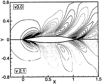
Figure 5. Wave Contours: Series 60.
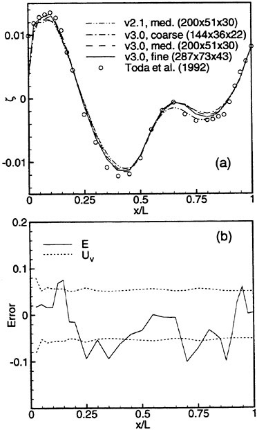
Figure 6. Hull Waterline: Series 60. (a) grid comparison; (b) validation

Figure 7. Off-Body Wave-Cut: Series 60. (a) grid comparison; (b) validation
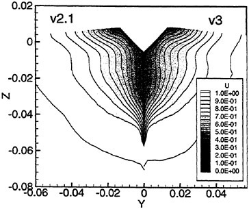
Figure 8. Nominal Wake: Series 60
DTMB Model 5415
Steady-flow solution for DTMB Model 5415 at full model scale Reynolds number (Re=1.39×10⁷) using v2.1 is presented for one grid system. In the following, resistance, wave profile on the hull, transom wave patterns, and nominal wake contours will be compared to the DTMB data (Ratcliffe, 1998). More detailed presentation and discussion can be found in Paterson et al. (1998).
A steady-flow solution at lower Reynolds number (Re=1.39×10⁶) using v3.0 is also presented for comparison purposes. Recall that for the v3.0 algorithm only the PISO pressure-velocity coupling was found to be capable of producing a converged solution for the DTMB 5415 geometry. The projection pressure-velocity coupling method was found to be unstable near the sonar dome and transom stern where a highly-skewed grid was required to resolve the complex geometric features.
Since the wave elevation outside the boundary layer is relatively insensitive to Reynolds number, qualitative comparison of wave elevation can be made even though the Reynolds number of the v3.0 solution is an order of magnitude lower. However, details of the boundary layer are Reynolds number dependent and only the v2.1 results for ship forces and nominal wake velocity contours are presented and compared to experimental data.
Comparison of the CT, CP, and CF to data and the ITTC friction line is shown in Table 8. Note that for Model 5415 the simulation is performed in the sunk and trimmed orientation as provided by DTMB. Given that Model 5415 and the Wigley hull both have similar magnitude E values for CT, the Series 60 conclusion concerning sinkage and trim effects appears justified.
Table 8. Comparison of forces (×10−3) for steady Model 5415 simulation, Fr=0.28, Re=1.39×10⁷.
|
|
S |
D |
E |
|
CT |
4.21 |
4.26 |
−1.2% |
|
CP |
2.51 |
2.48 |
+0.7% |
|
CF |
1.70 |
1.78 |
−1.9% |
Figure 9 shows comparison of the v2.1 and V3.0 solutions and the data, the latter of which includes uncertainty estimates which are shown as error bars. In general, agreement of both solutions with experimental data is excellent. Both solutions appear to accurately predict the bow wave peak and wave steepness at x/L=1.0. However, until verification analysis and assessment of numerical
uncertainty is completed, validation can not be assumed.
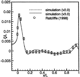
Figure 9. Hull Waterline: Model 5415.
Figure 10 shows a comparison of the computational grid and predicted wave-elevation contours in the near wake for v2.1 and v3.0 as well as comparison with experiment. Correct overall shape and location and extent of the “rooster tail” wave crest are correctly predicted for the v2.1 solution (Fig. 10c). However, the amplitude is grossly under predicted. Differences in peak wave elevation in the transom region between v2.1 and v3.0 using the same computational grid are most likely due to decreased numerical dissipation in the higher-order upwind scheme used in the v3.0 code. Alternatively, grid resolution can be increased in the transom stern region (Paterson et al., 1998) to improve resolution of the peak value in the v2.1 solution. The peak value of the “rooster tail” from the v3.0 solution (Fig. 10b) is much closer to the experimentally measured value.
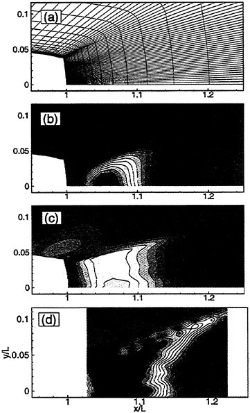
Figure 10. Transom Wave Pattern: Model 5415 (a) computational grid for v2.1 and v3.0 simulations, (b) simulation, CFDSHIP-IOWA, v3.0, (c) simulation, CFDSHIP-IOWA, v2.1, and (d) experiment, Ratcliffe (1998)
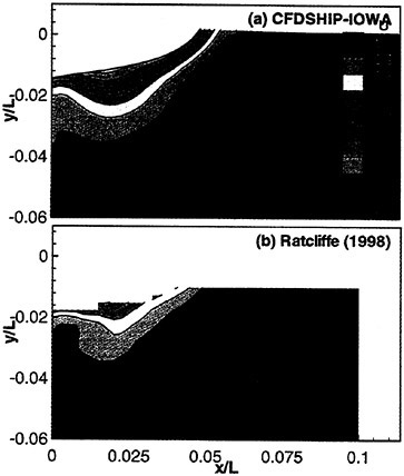
Figure 11. Nominal Wake: Model 5415
Finally, Figure 11 shows a comparison of the axial-velocity contours in the propeller plane, i.e., x/L=0.935. Again, good overall agreement is shown. Boundary layer thickness is correct as is the location of maximum thickness, or bulge, in the contours. The latter can be shown to have its origin at the sonar dome. However, the simulation does not sufficiently predict the narrowing of the boundary layer near the centerplane. Again, grid uncertainty assessment will aid in drawing conclusions and in making turbulence model changes and/or improvement if necessary.
5.2 Unsteady
Wigley Hull
Time-accurate simulations for the Wigley hull geometry in regular head waves are presented in this section. Time histories of ship forces are compared to available data (Journee, 1992) and the simulations of R&S. The diffracted wave pattern is compared to both R&S and the inviscid method SWAN from MIT (Kring and Sclavonous, 1997).
Time histories of total, pressure, and frictional resistance are shown in Figure 12(a). Figure 12(b)–(d) shows a comparison between the mean value of the fluctuating force and the value from the steady solution in calm seas, which is the effect due to streaming. The results from the v3.0 simulation show a small streaming effect for total and pressure resistance. Streaming effects are quantified and compared to R&S in Table 9.
Table 9. Comparison of streaming effects for unsteady Wigley hull simulation, Fr=0.3, Re=4.86×10⁶.
|
Method |
CT,STEADY |
CT,0 |
CT,STREAM |
|
v3.0 |
5.69 |
5.86 |
0.17 |
|
R&S |
5.65 |
5.97 |
0.19 |
The predicted value for the first harmonic of total resistance from the current study is compared to the validation study of R&S in Table 10, which shows validation at a level of 3.3% with simulation error of 2.4%. The difference between the predicted values from the simulation is 2.0% which is less than the numerical uncertainty estimates from R&S. As with the steady results, the unsteady total resistance is considered to be validated through comparison with the validation study of R&S.
Table 10. Comparison of first harmonic of resistance (×10−3) for unsteady Wigley hull simulation, Fr=0.3, Re=4.86×10⁶.
|
Force |
D |
SVer. 3 |
SRhee |
E*=SVer3.−SRhee |
|E| |
UV |
USN |
|
CT,1 |
5.39 |
5.34 |
5.26 |
2.0% |
2.4% |
3.3% |
2.2% |
A 3D perspective of the instantaneous wave field and hull for the time-accurate Wigley hull simulation at t=T is shown in Figure 13. The free surface mesh is colored by pressure.
A sequence in the evolution of the unsteady wave contours is shown in Figure 14 at each quarter period in time. The total wave elevation, ζ, is shown in the lower half while the diffracted wave elevation, ζdiff=ζ−ζ,0−ζ,outer, is shown in the upper half of the figure.
Figure 15 shows the diffracted wave pattern, predicted by v3.0 and R&S at t=T. Results are compared to those from the inviscid SWAN code. Quantitative agreement between v3.0 and SWAN can be seen while results from R&S show significant dissipation in the diffracted wave pattern. Differences are most likely due to solution of the
KFSBC. A separate free surface grid with larger near-wall spacing was used by R&S along with explicit dissipation.
DTMB 5415
Figure 16 shows preliminary results of instantaneous wave elevation at t=T/2 and t=T for time-accurate simulation of the DTMB 5415 in regular head waves using v2.1. Initial simulations of traveling waves provided motivation for developing the higher-order accurate, finite-difference code for efficient use of computational resources. Steady and time-accurate simulations of the DTMB 5415 using v3.0 are in progress. Critical issues under investigation for solution with the finite difference code include control and assessment of grid quality due to geometry complications at the bow and stern, selection of grid topology, and algorithmic robustness. Additional complications arise due to the shallow draft transom which could possibly become unwetted when simulating large amplitude incident waves. This could lead to problems in conforming the volume grid for certain grid topologies.
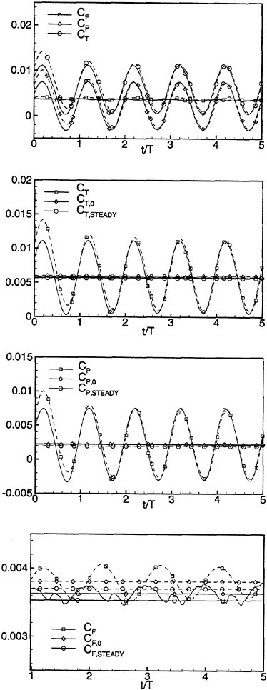
Figure 12. Unsteady Forces: Wigley Hull solid line –v3.0; dashed line –R&S (1998)
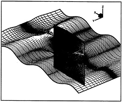
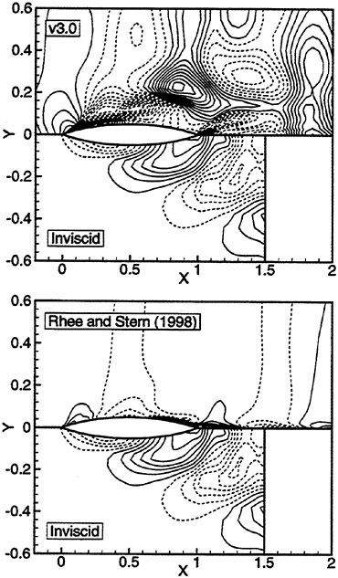
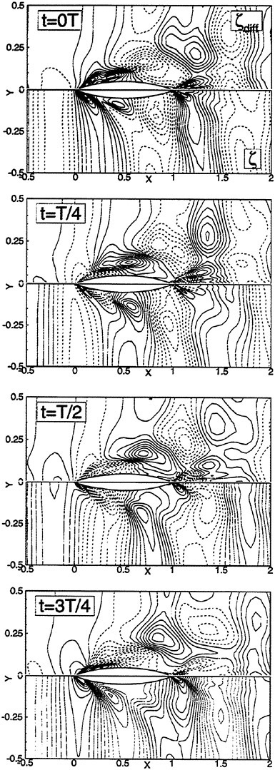
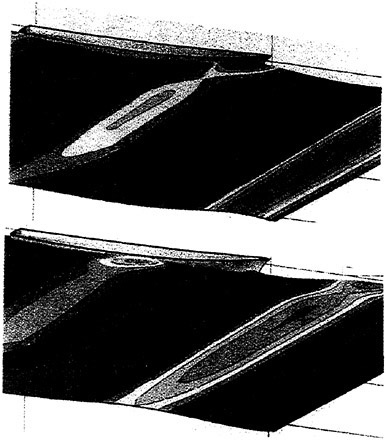
Figure 16. Instantaneous Wave Elevation Contours at t=T/2 and T: Model 5415.
6.0 CONCLUDING REMARKS
Development of version 3.0 of CFDSHIP-IOWA has been documented in this paper. This work has been motivated by the accuracy and efficiency requirements that are required for simulating naval combatants maneuvering in waves. Version 3.0 is based upon extensions of v2.1, which is a general purpose parallel multiblock RANS code using finite analytic discretization and the PISO algorithm. Accuracy is improved in the new v3.0 through the use of higher-order upwind finite differences. Steady flow verification and validation was presented for the code-development benchmark geometries which includes the Wigley hull, Series 60 CB=0.6 and the DTMB Model 5415. Unsteady flow results were presented for the Wigley hull and DTMB Model 5415. For the former, comparisons were made to Rhee and Stern (1998). For the latter, preliminary results using v2.1 were presented.
The overall structure of CFDSHIP-IOWA, which was designed for generality, modularity, and MPI-based parallel multiblock, provides a framework for code development and high-performance computing, implementation of v3.0 was relatively straightforward. The method shows significant improvement in comparison to v2.1, as demonstrated through reduced uncertainties and qualitative comparisons, for both accuracy and efficiency. Two methods for pressure/velocity coupling were tested; (i) projection and (ii) PISO. Use of the PISO method for pressure/velocity coupling was required for solution of flow over complex geometries (i.e., Model 5415 with sonar dome and transom stern) and is thus the preferred method to use in the v3.0 code.
The unsteady results for the Wigley hull show much promise for v3.0 in that it compares very well to the validated solutions of R&S. Moreover, due to higher-order discretization and artificial-dissipation-free formulation of the KFSBC solver, the diffraction wave pattern for v3.0 displayed less dissipation than R&S.
Current work is focusing on application of v3.0 for steady and unsteady flow for Model 5415 in conjunction with the DoD Challenge Project and the unsteady EFD at IIHR. Although this represents the first step in unsteady free-surface flows for practical naval geometries, the long-term goal is RANS simulation of seakeeping and maneuvering and ultimately simulation-based design.
7.0 ACKNOWLEDGEMENTS
This research was sponsored by Office of Naval Research grant N00014–96–1–0018 under the administration of Dr. E.P.Rood. The authors would like to acknowledge the DoD High Performance Computing Modernization Office and the DoD Challenge Program. Simulations were performed at the Naval Oceanographic Office Major Shared Resource Center using both the Cray T90 and the SGI Origin 2000.
REFERENCES
1. CFD Workshop Tokyo Proceedings, SRI, Ministry of Transportation, Tokyo, Japan. 1994.
2. Coleman, H.W. and Stern, F., “Uncertainties in CFD Code Validation,” ASME J. Fluids Eng., ASME J. Fluids Eng., Vol. 119, December 1997, Vol. 119, pp. 795–803.
3. Harlow, F.H. and Welch, J.E., “Numerical Calculation of Time-Dependent Viscous Incompressible Flow of Fluid with Free Surface,” Physics of Fluids (A), Vol. 8., 1965.
4. Journee, J.M.J., Experiments and calculations on four Wigley Hull Forms, Delft University of Technology, Ship Hydromechanics Laboratory, Report No. 909, 1992
5. Kring, D. and Sclavonous, P., Private Communiation, 1997.
6. McDonald, H., and Whitfield, D., “Self-Propelled Maneuvering Underwater Vehicles,” Proc. 21st ONR Symposium on Naval Hydro, Trondheim, Norway, 24–28 June 1996.
7. Newman, N., (1977), The MIT Press, Marine Hydrodynamics.
8. Paterson, E.G., Wilson, R.V., and Stern, F., (1998), “Verification/Validation for Steady Flow RANS Simulation of Model 5415,” 1st Symposium on Marine Applications of CFD, McLean, VA.
9. Paterson, E.G., Hyman, M., Stern, F., Carrica, P.M., Bonetto, F.J., Drew, D.A., and Lahey, Jr., R.T., “Near- and Far-Field CFD for a Naval Combatant Including Thermal-Stratification and Two-Fluid Modeling,” Proc. 21st ONR Symposium on Naval Hydro, Trondheim, Norway, 24–28 June 1996, 392–407.
10. Ratcliffe, T., “Validation and Verification of Free Surface RANS Codes,” Proceedings 22 ONR Symposium on Naval Hydrodynamics, Washington DC, 1998.
11. Rhee, S.H. and Stern, F., “Unsteady RANS Method for Surface Ship Boundary Layers and Wakes and Wave Fields,” 3rd Osaka Colloquium on Advanced CFD Applications to Ship Flow and Hull Form Design, Osaka, Japan, 25–27 May 1998.
12. Sotiropoulos, F. and Abdallah, S., “A Primitive Variable Method for Solution of 3D Incompressible Viscous Flow,” J. Comp Phys., Vol. 103, 1992.
13. Stern, F., Paterson, E.G., Tahara, Y., (1996), “CFDSHIP-IOWA: CFD Method for Surface Ship Boundary Layers and Wakes and Wave Fields,” IIHR Report #381.
14. Stern, F., Paterson, E.G., and Wilson, R.V.., (1998), “Guidelines and Recommended Practices for CFD Uncertainty Assessment,” IIHR Report in preparation.
15. Subramani, A., “Extensions of a Viscous Ship-Flow CFD Method for the Calculation of Sinkage and Trim,” M.S. Thesis, Department of Mechanical Engineering, The University of Iowa, 1996.
16. Tahara, Y. and Stern, F., “Large-Domain Approach for Calculating Ship Boundary Layers and Wakes and Wave Fields for Nonzero Froude Number,” Journal Computational Physics, Vol. 127, No. 2, September 1996, pp. 398–411, IIHR Reprint #1210.
17. Toda, Y., Stern, F., and Longo, J., (1992) “Meanflow measurements in the boundary layer and wake and wavefield of a Series 60 CB=0.6 ship model-part 1: Froude numbers 0.16 and 0.316,” J. Ship Research, Vol. 36, No. 4, pp. 360–377.
DISCUSSION
R.Lohner
George Mason University, USA
1. Why did you not do any Euler runs before jumping to RANS? One could have determined the accuracy of the method as compared to potential solutions (which you showed) in a much clearer manner.
2. You quoted a figure of 10 Cray T90 “flops” for a 52 processor SGI Origin 2000 run. What MFLOP-rate do you achieve on the T90?
AUTHORS’ REPLY
1. For a number of reasons, we do not routinely perform Euler calculations. Foremost is the fact that our interest is in simulation of unsteady turbulent flows for surface ships. As such, it is our opinion that conclusions about accuracy, robustness, and efficiency are best ascertained on the type of highly-stretched grids that are used in RANS simulations. It is important to recognize that the challenge of CFD for naval hydrodynamics is the resolution of both viscous and inviscid effects and the validation of a variety of quantities including wave field, turbulent boundary layer, forces and moments, and nominal wake.
We agree that it is important to verify algorithm performance. To that end, and as discussed in the paper, we have developed an approach which is based upon rigorous verification and validation methodology (Coleman and Stern, 1997; Stern, et al., 1998). As explained therein, order-of-accuracy may be obtained as part of the verification process where Richardson extrapolation and grid studies are used to estimate uncertainties due to spatial truncation errors.
Validation, on the other hand, is the process of comparing the simulation to a benchmark while taking into account the uncertainties. It should be noted that the validation method of Coleman and Stern (1997) separates numerical and modeling uncertainties and, as such, can be used to guide improvements and compare various models.
Finally, it is acknowledged that a potential-flow solution could theoretically be used for the wavefield validation benchmark given that its own uncertainty was assessed through the use of verification procedures. However, for geometries
such as Model 5415, it has recently been shown (Ratcliffe, 1998) that potential-flow methods have difficulty resolving both the bow and transom wave fields. As such, their utility in validating a general-purpose RANS code appears to be low, especially in comparison to available benchmark experimental data.
2. We appreciate this question since it allows us to further expand our discussion of the performance of CFDSHIP-IOWA. Timing experiments were recently performed using Model 5415 and 75 iterations on the 5-block grid system discussed in the paper. On the CRAY T90, versions 2.1 and 3.0 of the code achieve computational rates of 324 and 297 MFLOPs, respectively. The lower rate of version 3.0 is due to the use of penta-diagonal solvers instead of the tri-diagonal solvers used in v2.1.
In contrast, v2.1 on the SGI Origin 2000 achieves a serial computational rate of 39.4 MFLOPs. The 5-block system can be decomposed into 26-block and 52-block systems of approximately 20,000 and 10,000 points, respectively. On the 52-block grid system, a computational rate of 1570 MFLOPS has been achieved. This corresponds to a speedup of 40 over the serial calculation. Departure from linear speedup is due to both non-uniform block-size distribution, which can be remedied with a priori knowledge of parallel computing requirements, and the fact that not all of the blocks have free-surface boundaries which require solution of the KFSBC.
Computation of the Turbulent Flow Around a Ship Model in Steady Turn and in Steady Oblique Motion
A.Cura Hochbaum (Hamburg Ship Model Basin, Germany)
ABSTRACT
The turbulent flow around a ship model in steady turn as well as in steady oblique motion is computed solving the Reynolds-averaged Navier-Stokes equations for incompressible, steady flows. The finite-volume method used was extended to work on block-structured grids with non-matching interfaces. Velocity and pressure are coupled in a SIMPLE-like manner and Reynolds stresses are modelled with an algebraic turbulence model or with the k−ω model without wall functions. The free surface and related effects are neglected. In case of steady turning, inertial forces due to the computation in a ship-fixed coordinate system are treated explicitly and in both cases, boundary conditions were adapted to improve convergence. The computed flow fields for a Mariner class ship and for the Series 60 ship, both with CB=0.6, are mostly in close agreement with available experimental data, and the predicted sideforces and yaw moments on the hull always show the correct trend. Both turbulence models used yield almost the same forces but the k−ω model clearly predicts flow details more accurately. On the other hand, some numerical problems when using this model still remain.
INTRODUCTION
As a first step towards the future simulation of the flow around a manoeuvring ship, an in-house RANSE solver is being extended for the computation of the flow around a ship in oblique motion as well as moving in a steady turning circle with no drift at the midship section. The free surface as well as the dynamical trim, sinkage and heel are not taken into account during this exploratory phase. New questions concerning the choice of suitable boundary conditions and adequate grid topologies, as well as problems related to the computation in a non-inertial coordinate system arise now, in addition to old problems related to the insufficient robustness and accuracy of the technique used, [1]. Beyond these numerical aspects, it is also necessary to increase our knowledge about this kind of flow, which in many aspects is completely different than the flow in straight-ahead motion. Only few publications about oblique flow have been reported until now. An exception is the very instructive experimental work of Longo and Stern [2], which explains the most characteristic features of oblique flow and offers a very useful source for CFD validation. I’m not aware of similar analysis and data for a ship in steady turn. Unfortunately, the lack of flow field measurements for this case impeded the validation the computational results to greater extent. Computations for a ship in oblique motion and for a submarine in steady turn have already been reported, [3] [4], but as in case of the present work, they should be considered as a first step only. This paper is concerned with the problems of applying the method to these two simplified manoeuvres and with the discussion of the computed results.
MATHEMATICAL MODEL
The Reynolds-averaged Navier-Stokes equations with an eddy viscosity turbulence model for closure are solved. The governing equations in conservative differential form, in a non-inertial system, can be written:
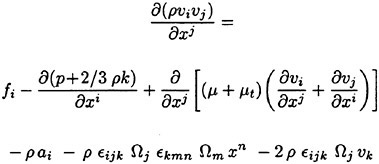
(1)
(2)
All indices run from 1 to 3. ρ is the water density, vi the mean velocity component in direction i, relative to the ship-fixed coordinate system, fi the component of an external volumetric force (e.g. gravity), p the mean pressure, k the turbulent kinetic energy, μ the molecular viscosity, μt the eddy viscosity and xi the Cartesian coordinate in direction i. The momentum equations (1) differ from those in an inertial system by the last three terms, i.e. the inertial forces steming from the acceleration and rotation of the coordinate system used, ai is the acceleration component of the system’s origin. The second term is the centrifugal force, Ωi being the angular velocity component, which is assumed to be constant, and ∈ijk the permutation symbol. The third term is the Coriolis force. Note that these terms don’t yield additional terms during the averaging process of the Navier-Stokes equations, because the velocity is involved only linearly. External forces are independent of the coordinate system used, and the constitutive equation used in (1) to approximate stresses by the deformation rates is valid in every system. Thus, no further modification of the momentum equations is necessary. Choosing a ship-fixed coordinate system yields to a steady flow (relative to this system) in both cases considered in this work. Thus, the time term is omitted in (1).
Two different turbulence models in their standard versions are used here. The very simple algebraic model of Cebeci and Smith [5], which has often been used for computing the flow around a ship model moving straight-ahead, is known to predict well the forces on the hull because no wall functions are used. On the other hand, it usually yields a rather poor wake prediction, because no turbulence transport is considered. Despite this drawback and somewhat surprisingly, the model seems to work well in the cases computed here. Alternatively, the k−ω model of Wilcox [6] is used, again integrating the flow down to the wall without wall functions. No special modification for the viscous sublayer and transition was implemented. In this model, the kinematic eddy viscosity arises from the quotient of the turbulent kinetic energy and the specific dissipation rate νt=μt/ρ=k/ω, for which two transport equations are solved.
At no slip boundaries, Wilcox recommends to place the first point at a non-dimensional wall distance ![]() and to have several further points with y+<2.5. In all these points, ω should be prescribed according to 6ν/(βy2), where ν is the kinematic viscosity, y the wall distance, and β=3/40 a model constant. In the present computations ω was enforced in the first point only, avoiding the calculation of the wall distance in more distant points, and the requirement concerning
and to have several further points with y+<2.5. In all these points, ω should be prescribed according to 6ν/(βy2), where ν is the kinematic viscosity, y the wall distance, and β=3/40 a model constant. In the present computations ω was enforced in the first point only, avoiding the calculation of the wall distance in more distant points, and the requirement concerning ![]() was satisfied only in case of the Series 60 ship. Note that, using this model, the necessary resolution is considerably higher than with the very popular k−ε model, where the cell thickness at the wall can be chosen 2 orders of magnitude larger. This leads to extremly large cell aspect ratios and consequently to more numerical difficulties in our case. The very smooth grids with strict spacing control at walls, which are required for convergence, are difficult to generate, representing a big disadvantage of this model for practical applications. Almost the same forces and moments on the hull are predicted with both turbulence models, but the predicted flow field is clearly better using the k−ω model. On the other hand, additional problems in achieving convergence were found when using this model, depending on the given values of k and ω in front of the ship. Only some combinations of these parameters, yielding reasonable length scales but too large eddy viscosities (e.g. 10 times molecular viscosity), led to convergence. Fortunately, no significant dependence of the solution on the given values was detected, but, due to the lack of convergence in several cases, no definite conclusion can be stated on this concern. Furthermore, the production of turbulent kinetic energy had to be limited to not exceed 20 times their dissipation for achieving convergence, following Deng and Visonneau [7].
was satisfied only in case of the Series 60 ship. Note that, using this model, the necessary resolution is considerably higher than with the very popular k−ε model, where the cell thickness at the wall can be chosen 2 orders of magnitude larger. This leads to extremly large cell aspect ratios and consequently to more numerical difficulties in our case. The very smooth grids with strict spacing control at walls, which are required for convergence, are difficult to generate, representing a big disadvantage of this model for practical applications. Almost the same forces and moments on the hull are predicted with both turbulence models, but the predicted flow field is clearly better using the k−ω model. On the other hand, additional problems in achieving convergence were found when using this model, depending on the given values of k and ω in front of the ship. Only some combinations of these parameters, yielding reasonable length scales but too large eddy viscosities (e.g. 10 times molecular viscosity), led to convergence. Fortunately, no significant dependence of the solution on the given values was detected, but, due to the lack of convergence in several cases, no definite conclusion can be stated on this concern. Furthermore, the production of turbulent kinetic energy had to be limited to not exceed 20 times their dissipation for achieving convergence, following Deng and Visonneau [7].
The eddy viscosity hypothesis used to approximate the Reynolds stresses in the momentum equations may be even worse than usual in case of a rotating system because of the increased turbulent anisotropy. No changes due to the non-inertial coordinate system used are imperative in the transport equations for the turbulent parameters k and ω. Nevertheless, the exact equations for the Reynolds stresses do contain extra terms due to the system rotation, indicating that the turbulence model should take into account the increased anisotropic turbulence features. Despite this is not expected to be crucial in our case, it should be analized in future.
COMPUTATIONAL GRID
Grids consisting of a single structured block are often not suitable for applications with high geometric complexity, e.g. for a ship with appendages. Most Navier-Stokes solvers now can deal with block-structured grids or even with unstructured grids. The latter offer the biggest flexibility when generating grids, simplifying considerably this very time consuming process. On the other hand, the fact that unstructured grids are less suitable to resolve the near wall region, weakens their advantage. Thus, the in-house Navier-Stokes solver NEPTUN was extended to work on block-structured grids. Fig. 1 shows the inner blocks, at the port side of a ship. There is considerably more flexibility to handle complex geometries than in the past now, because non-matching interfaces are allowed, i.e. cell vertices of adjacent blocks must not coincide at common faces. Choosing the proper topology and resolution in each region of the computational domain leads to a more economical distribution of cells and avoids typical singularities of single block grids.
Fig. 2 shows part of the grid at the port side of a Mariner ship. Only every second grid line is depicted. The grid has been opened at a non-matching interface in the stern to show a topology change from O-type into Η-type in the neighbourhood of the hull. O-type grids are good for regions where offsets are U-shaped or have a flat bottom, e.g. at midships, but when offsets become more and more V-shaped and in the wake, Η-type grids are preferable. The whole grid consists of more than 40 blocks in this case, including both ship sides, with about 480000 cells altogether. However, the block partitioning is not only justified by the topology, but also for simplifying the grid generation. Non-matching interfaces are restricted to be on planes at the moment, and each cell side on an interface has to fully consist of cell sides or parts of cell sides of the neighbour blocks. These constraints do not represent a big limitation in practice and allow a fully automatic determination of all information needed for the computation.
The grid completely fits the body now, including stem, post and rudder contours, Fig. 3. This feature is more important than in the straight-ahead case because the usually resulting steps could otherwise lead to flow separation at a wrong position on a full stern or on a bulbous bow. In order to generate the grid on the hull, a 2D elliptic grid-generator was extended for surface grids, based on the formulae of Gauss and Beltrami, [8]. Additionally, an iterative determination of control functions to (nearly) achieve orthogonality and a desired spacing at boundaries was implemented as specified by Sorenson in [8]. This does not guarantee the resulting grid to lie exactly on the hull, nor to hold the intended spacing exactly. Thus, the grid points are subsequently projected onto the hull and shifted to attain the required spacing, if desired. This method yields better grids than in the past, but it is not robust enough and requires several attempts until the grid is satisfactory. It can also be used to generate 3D grids surface by surface (not necessarily planes) when control of grid lines is crucial. Fig. 4 shows the O- and Η-type grid surfaces generated in this way at a transverse section in the afterbody of the Series 60 ship, where the grid changes it’s topology.
NUMERICAL METHOD
The transport equations for momentum and mass (RANSE), and for turbulent parameters if necessary, are discretized in a finite-volume manner, where all unknowns are stored for the cell centers. Mass fluxes at cell sides are determined using the technique of Rhie and Chow [9]. Convective terms are approximated with the Linear Upwind Differencing Scheme (LUDS), and diffusive terms with the Central Differencing Scheme (CDS). The SIMPLE method is used to iteratively solve the resulting set of non-linear equations. The method was described in detail in [10]. Only some aspects concerning the new multi-block technique and the boundary conditions for oblique flow and steady turn will be described here.
The information about the neighbouring blocks and composition of cell sides on block interfaces computed beforehand is used when calculating mass and momentum fluxes at these cell sides. Consider the eastern side of cell P, lying at a block interface, Fig. 5. There are seven neighbouring cells Ei from one or more adjacent blocks involved in the composition of it’s area. Whenever values of variables in the cell center of the missing usual eastern neighbour Ε are needed, they are determined using the following area-weighted interpolation:
(3)
Φ may be a velocity component, the pressure or pressure correction, etc. The contribution si of cell Ei to the area of the considered cell side takes values between 0 and 1, the sum of all contributions being 1. Values in the missing more distant eastern cell center EE, not shown in Fig. 5, as well as the interpolation factors used for linear interpolation at the cell side are also determined in this way. It would be necessary to determine in this way also products of interpolation factors and flow variables, to fully retain the conservativeness of the numerical method when non-matching interfaces are present. Despite this was not implemented, computations show negligible global losses of mass and momentum.
In order to prevent the overall convergence to slow down, i.e. the number of outer iterations to increase due to the partitioning of the domain into blocks, values at interfaces are updated during the inner iterations of velocities and pressure correction. When a relaxation sweep is completed in a block, the values needed for the neighbouring blocks are calculated using (3) before going on with the next block. Especially the exchange of pressure corrections between blocks in every inner iteration is crucial for convergence. Indeed, no slow down of convergence compared to calculations on single block grids was detected. The solution remains smooth at interfaces even where large gradients occur, provided similar resolution has been chosen in adjacent blocks.
The inertial forces due to the computation in a ship-fixed coordinate system are treated as extra sources in the momentum equations when computing steady turns. Because convergence didn’t deteriorate doing so, no special treatment of these terms was necessary, other than in applications were the angular velocity is very large. Computations of steady turns converged even faster than oblique flows. Note that, even though inertial forces are moderate for a ship in steady turn, the results are completely wrong if they are neglected.
Due to the asymmetric flow considered, both sides of the ship have to be discretized, doubling (at least) the usual number of cells and increasing the computing time by a factor of about 3 compared to straight-ahead ship motion. It is particularly advantageous to keep the computational domain small in this case, as long as the solution does not deteriorate doing so. The outer boundaries of this domain are artificial borders, and the (non-physical) boundary conditions chosen there can be decisive for the convergence. As can be noticed in Fig. 2, the outer border of the domain consists of vertical planes at port and starboard side, a horizontal plane at the bottom and fore and aft planes. Referred to the ship-fixed coordinate system, Fig. 6, the fore boundary lies at x/L=1 and the aft boundary at x/L=−1.5, L being the ship length. The side boundaries are at y/L=±1, the waterplane at z/L=0 and the bottom at z/L=1. Tests with larger computational domains did not yield significantly different results. A reduction of the domain sizes in transverse and vertical directions to 1/2 each yielded only minor changes in sideforce and yaw moment, but the longitudinal force (resistance) was predicted 5%. larger.
For oblique motion and steady turn in unconfined water, the same grid could be used. For all considered drift angles and yaw rates only the boundary conditions were changed. For both cases, the freestream fluid velocities relative to the ship-fixed system are:
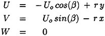
(4)
Uo is the speed of, and β the drift angle at the system’s origin. The yaw rate r yields the angular velocity components Ω1=Ω2=0, Ω3=r in (1). Freestream velocities (4) are set at the fore boundary and bottom, and the freestream pressure p0 is set at the aft boundary. The waterplane is assumed to be a rigid symmetry plane. Other than in the straight-ahead case, water can enter and/or leave the computational domain through the lateral boundaries, as illustrated in Fig. 7. Original convergence difficulties for large drift
angles and yaw rates could be removed using a “mixed boundary condition”. It consists in setting the freestream values only for the convection velocities (mass fluxes) in the convective fluxes, where the fluid leaves the domain through the cell side considered. The convected velocities are then still extrapolated by LUDS. Where the fluid enters the domain, all velocities are given as usual. The mixed condition is used at the leeward lateral boundary when computing oblique motions, and at the lateral boundary toward the center of the circle when computing steady turns. The freestream velocities are set at the windward lateral boundary in the former case, and the freestream pressure is set at the lateral boundary opposite to the center of the circle, in the latter case. Convergence slows down for increasing drift angle β as well as for increasing non-dimensional yaw rate r′=rL/Uo. This is due to the more complicated flow with less dominating main flow direction. Nevertheless, converged results, i.e. reduction of initial momentum and mass residuals by 4 orders of magnitude, could be obtained with usual underrelaxation factors, e.g. 0.6 for velocities and 0.3 for pressure.
APPLICATIONS
Results for the Mariner ship
Computations were done for a 6.437 m model of the Mariner ship at Reynolds number Rn=107 and Froude number Fn=0.2, in steady oblique motion as well as performing a turning circle with constant speed and zero drift angle at the midship section. The principal dimensions at full scale are Lpp=160.93 m, Β=23.17 m, Τf=6.85 m, Ta=8.075 m and CB=0.6, [11]. The computed results are compared with experimental data obtained with the Computarized Planar Motion Carriage and in oblique towing tests at the Hamburg Ship Model Basin, [12] and [13].
The rudder was approximated by a zero-thickness plate in the computations, Fig. 3, and the bilge keels present in the model were not taken into account. The finest grid had about 480000 cells. Computations on two coarser grids with 60000 and 7500 cells obtained from the former grid by removing every second line in each direction were done to check grid convergence of the solution. The differences between results on two subsequent grids decreased satisfactorily. Despite no grid independece could be achieved with the available hardware (differences of several percent occurred between the solutions on the medium and fine grid), further refinement is expected to change the predicted forces by less than 3%. Interestingly, the results on the medium grid already show most of the flow features of the fine grid solution. Computations with both turbulence models mentioned before were performed. Nevertheless, the chosen grid spacing yielding ![]() in most parts of the hull was somewhat too large for the k−ω model. Results obtained with the algebraic model are shown here, except where otherwise noted. About 600 SIMPLE iteration steps were necessary to achieve convergence, Fig. 10, demanding a CPU time of 15 hours on a normal workstation. The required memory was 155 MB.
in most parts of the hull was somewhat too large for the k−ω model. Results obtained with the algebraic model are shown here, except where otherwise noted. About 600 SIMPLE iteration steps were necessary to achieve convergence, Fig. 10, demanding a CPU time of 15 hours on a normal workstation. The required memory was 155 MB.
Most features of the flow around a ship in oblique flow completely differ from those of a ship moving steadily ahead. The symmetric pressure distribution on the hull becomes extremely asymmetric, yielding a sideforce and a yaw moment. Fig. 8 shows the pressure coefficient ![]()
![]() on the hull, at a drift angle β=12°. The stagnation point shifts to the port side of the bulbous bow, and the point of attack of the sideforce can be discerned to lie in the forebody, yielding a positive yaw moment.
on the hull, at a drift angle β=12°. The stagnation point shifts to the port side of the bulbous bow, and the point of attack of the sideforce can be discerned to lie in the forebody, yielding a positive yaw moment.
The skin friction coefficient ![]()
![]() τ being the magnitude of the wall shear stress, vanishes at the starboard side of the bow near the waterplane, indicating that flow separation occurs, Fig. 9. Velocity vector plots at horizontal cuts, not shown here, showed a recirculation zone extending from the stem to the middle of the region where Cf=0 in Fig. 9. Although this couldn’t be verified yet, it seems very plausible because of the sharp entry angles of the waterlines in the upper part of the bow. A similar effect was predicted at the bow of the Series 60 ship, the phenomenon being somewhat less pronounced and more two-dimensional there. Because no bulb is present in that case, the separation zone extends almost to the keel, and re-attachment occurs along a rather vertical line lying still upstream of the turbulence stimulators present in the ship model. No flow recirculation was detected elsewhere (including the stern), but 3D flow separation occurs in large regions. While the cross flow separates, the main flow remains attached. The skin friction can even reach maximum values there, as happens along the bilge at the starboard side in Fig. 9.
τ being the magnitude of the wall shear stress, vanishes at the starboard side of the bow near the waterplane, indicating that flow separation occurs, Fig. 9. Velocity vector plots at horizontal cuts, not shown here, showed a recirculation zone extending from the stem to the middle of the region where Cf=0 in Fig. 9. Although this couldn’t be verified yet, it seems very plausible because of the sharp entry angles of the waterlines in the upper part of the bow. A similar effect was predicted at the bow of the Series 60 ship, the phenomenon being somewhat less pronounced and more two-dimensional there. Because no bulb is present in that case, the separation zone extends almost to the keel, and re-attachment occurs along a rather vertical line lying still upstream of the turbulence stimulators present in the ship model. No flow recirculation was detected elsewhere (including the stern), but 3D flow separation occurs in large regions. While the cross flow separates, the main flow remains attached. The skin friction can even reach maximum values there, as happens along the bilge at the starboard side in Fig. 9.
The computed velocity field in cross section x/L=0.3 for the Mariner ship in steady turn
at r′=0.5 showed very similar patterns to that in oblique motion, including the cross flow separation mentioned before, Fig. 11. The situation on the afterbody is different because the local drift angle changes sign at the midship section, resulting in a more aligned flow there. The oblique flow at β=12°, the same angle as the local drift angle at x/L=−0.4, showed a very pronounced vortex at the leeward side in contrast to the very weak one in Fig. 11.
The computed transverse velocity field in the propeller disk for the Mariner ship in oblique motion at β=12° agrees well with the measurements of Laudan [13], Fig. 13. The circles corresponding to the measurements are shown together with the computed results for reference. The measured velocity field is rather homogeneous on the windward side (on the right hand here) and shows a very pronounced vortex on the leeward side. Computed results are somewhat better using the k−ω model (bottom), but the features mentioned before are predicted satisfactorily also with the algebraic model (middle), the vortex being somewhat weaker in this case. The computations are clearly able to predict the changes in the position of the vortex for different drift angles, e.g. for β=18°, Fig. 14. This is rather surprising, and could be the result of a more convection-dominated flow than in the straight-ahead case.
Although the rudder was approximated by a zero-thickness plate, the variation of the non-dimensional sideforce ![]() and non-dimensional yaw moment
and non-dimensional yaw moment ![]() with drift angle β and non-dimensional yaw rate r′ is predicted well, as shown in Fig. 12 and 15. The dashed lines in Fig. 12 correspond to computations without a rudder. As expected, significant changes in Y′ and N′ occur then, showing that consideration of appendages is crucial for a manoeuvring ship. Interestingly, the errors are much smaller for both sideforce and moment for the steady turning motion (Fig. 15), but this may be only coincidence. Note that this encouraging prediction of forces and moments was not accurate enough for predicting the yaw stability index C′, [14]. For this purpose, the free surface and all appendages should be taken into account.
with drift angle β and non-dimensional yaw rate r′ is predicted well, as shown in Fig. 12 and 15. The dashed lines in Fig. 12 correspond to computations without a rudder. As expected, significant changes in Y′ and N′ occur then, showing that consideration of appendages is crucial for a manoeuvring ship. Interestingly, the errors are much smaller for both sideforce and moment for the steady turning motion (Fig. 15), but this may be only coincidence. Note that this encouraging prediction of forces and moments was not accurate enough for predicting the yaw stability index C′, [14]. For this purpose, the free surface and all appendages should be taken into account.
Results for the Series 60 ship
Computations were done for a 3.048 m model of the Series 60 CB=0.6 ship at Reynolds

Figure 23. Convergence of predicted forces with grid resolution. Series 60 Ship at β=10°.
number Rn=2.67 106 and Froude number Fn=0.16 in steady oblique motion. The principal dimensions at full scale are Lpp=121.92 m, Β=16.26 m, Τ=6.50 m, [15]. The computed results are compared with experimental data obtained in oblique towing tests at the Iowa Institute of Hydraulic Research, [2].
A similar grid to that used for the Mariner ship with a total number of cells Ν≈480000 was used. More care was taken in placing the innermost cell centers in this case, yielding ![]() almost over the entire hull. Computations on two systematically coarsed grids show satisfactory convergence behaviour, Fig. 23. Nevertheless, the difference between the predicted resistance coefficients CT on the medium and fine grid is still 5%. Further grid refinement is expected to change the predicted resistance by less than 3%, and the sideforce and yaw moment by less than 2%. Computations were performed with both turbulence models, algebraic and k−ω without wall functions. Results obtained with the latter model are shown here, except where otherwise noted. As mentioned before, convergence could only be achieved by choosing freestream values for k and w such that a relatively large eddy viscosity results. About 800 SIMPLE iteration steps were necessary to achieve convergence, demanding about 22 hours on a normal workstation. Most of the results do not change any more after 400 iteration steps, and no significant changes occur after 600 steps.
almost over the entire hull. Computations on two systematically coarsed grids show satisfactory convergence behaviour, Fig. 23. Nevertheless, the difference between the predicted resistance coefficients CT on the medium and fine grid is still 5%. Further grid refinement is expected to change the predicted resistance by less than 3%, and the sideforce and yaw moment by less than 2%. Computations were performed with both turbulence models, algebraic and k−ω without wall functions. Results obtained with the latter model are shown here, except where otherwise noted. As mentioned before, convergence could only be achieved by choosing freestream values for k and w such that a relatively large eddy viscosity results. About 800 SIMPLE iteration steps were necessary to achieve convergence, demanding about 22 hours on a normal workstation. Most of the results do not change any more after 400 iteration steps, and no significant changes occur after 600 steps.
The k−ω model yields a better prediction of flow details even though the algebraic model works surprisingly good. Fig. 16 shows the predicted transverse velocity field in a cross section
at x/L=0.1, upstream of the midship section. As opposed to the k−ω model, the algebraic model (top) is not able to predict the keel vortex present in experiment, see also Fig. 21. Because of the relatively small Reynolds number, laminar effects are expected to be more important than usual in this case. Note that the ship model had a row of cylindrical studs at x/L=0.45, 5% L from the forward perpendicular to initiate the turbulence transition, [2]. Considering a laminar flow until this section is reached and switching on the turbulence model there, the results obtained are somewhat better than without doing so and are shown in the following. Note that the k−ω model would predict transition much earlier, [6].
The resistance coefficient CT, based on the wetted area of the model at rest, and the nondimensional sideforce ![]() and yaw moment
and yaw moment ![]() are compared with measurements in Fig. 18. The overall agreement is satisfactory. It may be noted that the free surface and related effects were not considered in the computations, nevertheless the model was free to heave, pitch and roll. Although the Froude number considered is quite small, these effects probably play a more important roll in oblique motion.
are compared with measurements in Fig. 18. The overall agreement is satisfactory. It may be noted that the free surface and related effects were not considered in the computations, nevertheless the model was free to heave, pitch and roll. Although the Froude number considered is quite small, these effects probably play a more important roll in oblique motion.
Contours of computed axial velocity and transverse velocity fields in selected cross sections are compared with the measurements of Longo and Stern for a drift angle β=10°. The overall agreement is quite good. Somewhat unexpected, many of the very complicated flow features present in experiment and described in [2] were predicted well by the computations.
Both the forebody keel and bilge vortices can be seen clearly in the computed velocity distributions shown in Fig. 19 and 21. Differences between the velocity contours in the neighbourhood of the waterplane at the starboard side in Fig. 19 can be explained clearly by the neglect of the free surface in the computations. The three sections showed there, accidentally coincide with troughs at the starboard (leeward) side of the ship as can be seen in the measured wave elevation, Fig. 17. The axial coordinate has it’s origin at the forward perpendicular there. The deepening of the free surface causes an acceleration of the axial velocity leading to a concentration of the contours at the upper part of the cross sections. At section x/L=0.1 in Fig. 21, the slight improvement compared with Fig. 16 can be recognized.
The agreement is also very convincing in the afterbody and wake as shown in Fig. 20 and 22. In contrast to those in the forebody, these sections are in regions where the wave elevation is positive and small at the starboard side, Fig. 17. Thus, less wave induced effects are present here. The developement and shedding of the bilge vortex is predicted well, although less pronounced than in experiment. Even the small secondary vortex near the waterplane at x/L=−0.6 in the wake of the ship can be recognized in the results in Fig. 22, despite of the rather coarse grid resolution chosen there.
CONCLUSIONS
Results of the computation of the turbulent flow around the Mariner ship in steady turn and oblique motion and around the Series 60 ship CB=0.6 in oblique motion showed close agreement with experimental data. The method was able to predict complex flow phenomena like 3D separation and vortex shedding in these cases. Further validation is necessary to take definite conclusions about the quality of the results, especially in case of steady turn. The comparison of other cases with experiments will shed more light on this matter. For a more accurate prediction of forces and moments on the hull, the free surface and all appendages should be considered. The implemented multi-block technique, allowing non-matching interfaces, offers enough flexiblity to take ship appendages into account in future. The k−ω model used seems to be a good alternative to other turbulence models used in practice, provided some numerical questions can be cleared, becoming more robust.
ACKNOWLEDGEMENT
This work was supported by the German Ministry of Education, Research and Technology.
References
[1] Cura Hochbaum, A. and Laudan, J. (1996), “Computation of Turbulent Ship Flow,” 1st South African Conference on Applied Mechanics (SACAM’96), Midrand, SouthAfrica.
[2] Longo, J. and Stern, F. (1996), “Yaw Effects on Model-Scale Ship Flows,” 21th ONR
Symposium on Naval Hydrodynamics, Trondheim.
[3] Patel, V.C., Ju, S. and Lew, J.M. (1990), “Viscous Flow Past a Ship in a Cross Current,” 18th ONR Symposium on Naval Hydrodynamics, Ann Arbor.
[4] Sung, C.-H., Fu, T.-C., Griffin, M. and Huang, T. (1996), “Validation of Incompressible Flow Computation of Forces and Moments on Axisymmetric Bodies Undergoing Constant Radius Turning,” 21th ONR Symposium on Naval Hydrodynamics, Trondheim.
[5] Cebeci, T. and Smith, A.M.O. (1974), “Analysis of Turbulent Boundary Layers,” Academic Press, New York.
[6] Wilcox, D.C. (1993), “Turbulence Modeling for CFD,” DCW Industries, La Cañada, California.
[7] Deng, G. and Visonneau, M. (1996), “Evaluation of Eddy Viscosity and Second-Moment Turbulence Closures for Steady Flows Around Ships,” 21th ONR Symposium on Naval Hydrodynamics, Trondheim.
[8] Thompson, J.F., Warsi, Z.U.A. and Wayne Mastin, C. (1985), “Numerical Grid Generation—Foundations and Applications,” North-Holland, New York.
[9] Rhie, C.M. and Chow, W.L. (1983), “Numerical Study of the Turbulent Flow Past an Airfoil with Trailing Edge Separation,” ΑΙΑA Journal, Vol. 21, No. 11.
[10] Cura Hochbaum, A. (1994), “A Finite-Volume Method for Turbulent Ship Flows,” Ship Technology Research, Vol. 41, pp. 135–148.
[11] Morse, R.V. and Pride, D. (1961), “Maneuvering Characteristics of the Mariner Type Ship (USS Compass Island) in Calm Seas,” Sperry Gyroscope Co., Syosset N.Y., Publ. No. GJ-2232–1019.
[12] Oltmann, P. and Wolff, K. (1979), “Vergleichende Untersuchung über das Manövrierverhalten des Mariner-Standardschiffes,” University of Hamburg, IfS Report 385.
[13] Laudan, J. (1977), “Zweiquadrantenmes-sungen bei Schräganströmung hinter einem Schiffsmodell,” Hamburg Ship Model Basin Report 1508.
[14] Brix, J. (1993), ed., “Manoeuvring Technical Manual,” Seehafen Verlag, Hamburg.
[15] Todd, F.H. (1963), “Series 60 Methodical Experiments with Models of Single-Screw Merchant Ships,” David Taylor Model Basin Report 1712.
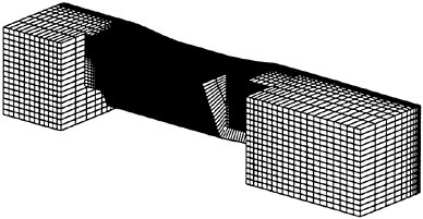
Figure 1. Inner blocks at the port side of a ship.
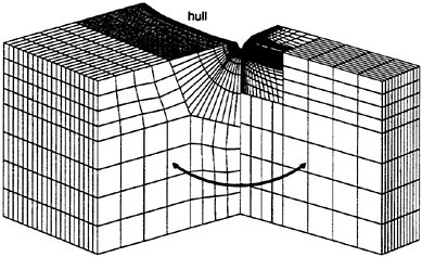
Figure 2. Partial view of a block-structured grid opened at a “non-matching interface”.
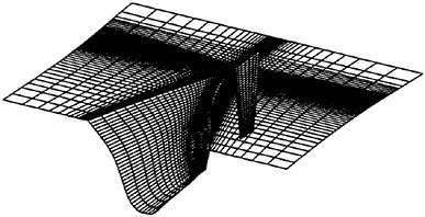
Figure 3. Grid with zero-thickness rudder at the stern of the Mariner Ship.
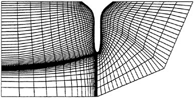
Figure 4. Grid topology change at offset in afterbody of Series 60 ship. Here depicted: O-type at starboard and Η-type at port side.

Figure 5. Cell Ρ at an interface and its neighbours in the adjacent block(s).
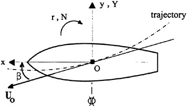
Figure 6. Ship-fixed coordinate system.
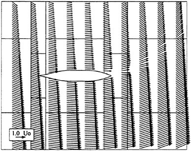
Figure 7. Relative velocity field on waterplane around a ship in steady turning motion.
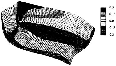
Figure 8. Pressure coefficient on forebody. Mariner ship at Rn=107, β=12°.
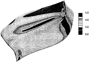
Figure 9. Skin friction coefficient ·103 on forebody. Mariner ship at Rn=107, β=12°.

Figure 10. Convergence history of oblique flow computation. Mariner Ship at drift angle β=12°.
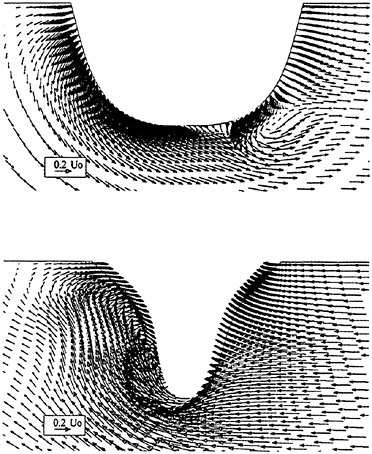
Figure 11. Computed transverse velocity field at offsets x/L=0.3 (top) and x/L=−0.4 (bottom). Mariner ship at Rn=107, steady turn r′=0.5.
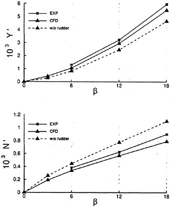
Figure 12. Measured and computed normalized sideforce and yaw moment on Mariner ship hull in oblique flow, Rn=107.
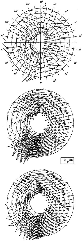
Figure 13. Measured (top) and computed transverse velocity field in propeller plane. Middle: algebraic model. Bottom: k−ω model. Mariner Ship at drift angle β=12°, Fn=0.20, Rn=107.
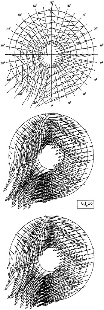
Figure 14. Measured (top) and computed transverse velocity field in propeller plane. Middle: algebraic model. Bottom: k−ω model. Mariner Ship at drift angle β=18°, Fn=0.20, Rn=107.
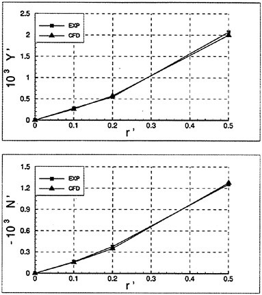
Figure 15. Measured and computed normalized sideforce and yaw moment on Mariner ship hull in steady turn, Rn=107.
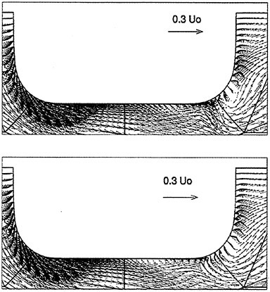
Figure 16. Transverse velocity field at x/L=0.1, computed with algebraic (top) and k−ω turbulence model (bottom).
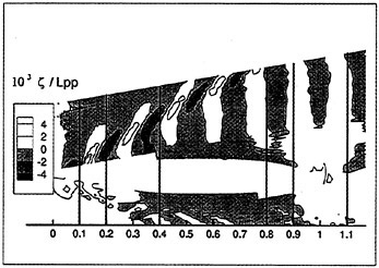
Figure 17. Measured wave elevation, Longo and Stern (1996). Series 60 Ship CB=0.60 at drift angle β=10°, Fn=0.16, Rn=2.67 106.
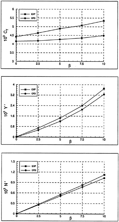
Figure 18. Measured and computed normalized forces and yaw moment vs. drift angle. Series 60 Ship CB=0.60, Fn=0.16, Rn=2.67 106.
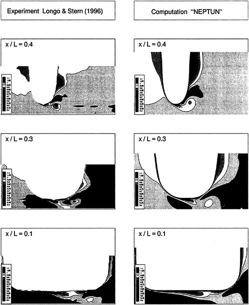
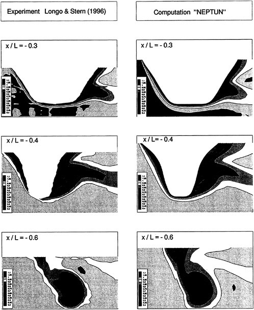
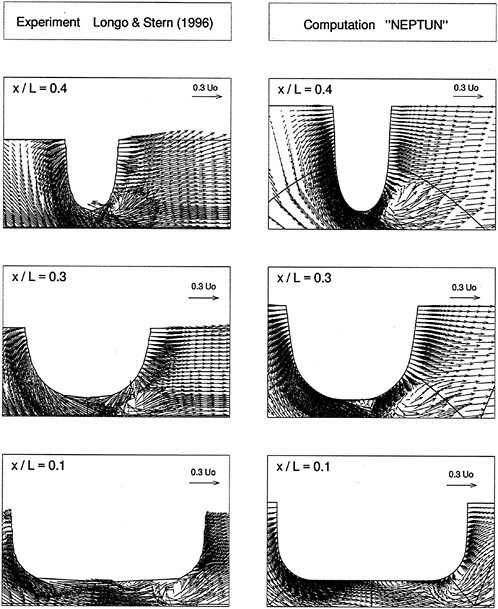
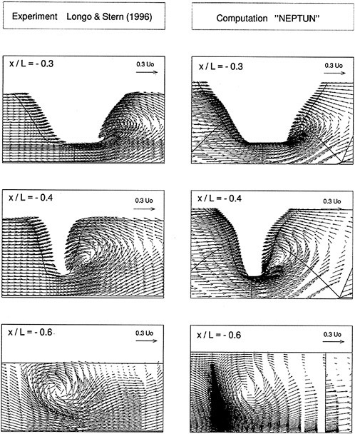
DISCUSSION
T.Hino
Ship Research Institute, Japan
The governing equation (1) is written in the conservation form for the inviscid and viscous terms. However, the source terms associated with the coordinates rotation are treated in the non-conservative manner. This would become a source of numerical errors, since the discretization of the Coriolis force and the centrifugal force do not necessarily balance with the discretized convection terms for a uniform flow. Did the author treat the source terms in a special way as Alessandrini et al. did in their paper presented in this Symposium?
The second question is concerned with the turbulence model. The κ-ω model in the present code seems to do an extremely good job for the complex flow fields of drift and turning motions. On the other hand, the author reported the numerical difficulty of this turbulence model. Also, it is well known that the flow field with the original κ-ω model is strongly dependent on the free-stream value of ω. I would like to have the author’s opinion regarding the remedy for these defects of the model.
AUTHOR’S REPLY
The inertial forces were simply treated as source terms and discretized in a non-conservative manner. This could in fact be a source of numerical errors. The unbalanced discretization of these terms and convection terms in a uniform flow arises from the interpolation/extrapolation of velocities at cell faces along curvilinear gridlines, and would not occur on a rectilinear grid. Although the effects on the results are probably small, because of the relatively small angular velocity in steady turns, I agree with Dr. Hino in that the inertial forces should be treated more carefully and thank him for the helpful tip.
The numerical difficulties using the κ-ω turbulence model are due to the low grid quality in some critical regions of the computational domain (the smoothness and spacing required cannot be guaranteed everywhere) as well as to some dependence of convergence on the free-stream values of κ and ω. Despite the well-known dependence of the calculated eddy viscosity on the ω value, I have not detected any considerable influence on the more interesting results, e.g., the predicted forces and wake distribution. Due to the good results obtained with the κ-ω model, it would be worthwhile to try to mitigate its drawbacks. A turbulence model proposed by Menter [1], which avoids the dependence of the κ-ω model on free-stream values, blending it with a modified κ-ε model used outside of the boundary layer, seems to be an attractive alternative.
Reference
[1] Menter, F.R. (1994), “Two-Equation Eddy-Viscosity Turbulence Models for Engineering Applications,” AIAA Journal, Vol. 32, No. 8.
DISCUSSION
H.Söding
Technical University Hamburg-Harburg, Germany
Maneuvering predictions are required by IMO, but present means of doing so in practice are quite crude. One of the difficulties is the sensitivity of the maneuvering characteristics to small differences between hull forces in drift motion and those in yaw motion. This sensitivity causes large errors in predicted overshoot angles: More than 100% error is normal in some methods used today, although better predictions are possible even with relatively simple means like slender body theory and lifting line theory if theoretical considerations are suitably combined with empirical corrections. This holds for most of the maneuvering characteristics except for the yaw stability index C which seems nearly unpredictable due to its extreme sensitivity.
Essential improvements of the present half-empirical maneuvering predictions seem possible only by applying viscous flow calculations for the maneuvering hull with rudder and some equivalent of the propeller. The author has presented a very successful application of his RANS code to maneuvering ships. The work is held to be a great step forward towards a satisfactory prediction. Clearly several improvements are still required: less manual effort in mesh generation, more robust solution, inclusion of bulge keels, propeller action, instationary motions, and for higher speed also heel, squat and free surface deformation. Further, a method has to be developed for simulating arbitrary maneuvers by using force coefficients derived from a few computations only. The results presented here indicate that it is very worthwhile to proceed in this direction.
It would be interesting if the author could present also the differences of non-dimensional forces between
model and full scale for a few cases, to estimate whether the difference of, say, up to 17% between his computations and model experiments is less or more than the error of full-scale predictions based on model force coefficients.
AUTHOR’S REPLY
Thank you Prof. Söding for your comments. The sensitivity of the yaw stability index which you mention supports the statement in my paper concerning the poor prediction of C’. I expect predictions to become more precise when computations include the free surface, dynamical shrinkage, trim and heel, as well as all appendages. But even then, a good prediction of C’ would only be useful for ships which don’t significantly heel in oblique motion. For other cases, the slope of the reverse spiral test curve at the origin should be taken as a measure of yaw stability, thus requiring a more complex computational procedure.
So far, computations were only done for model scale, and therefore no comparison of predicted nondimensional forces for model and full scale have been made. It might be of interest though that the computed side forces for the Mariner ship at ß=12° differ by roughly 20% when considering inviscid (Euler) flow instead of viscous flow at model scale. The differences due to the different Reynolds numbers of ship and model are expected to be smaller but still significant. On the other hand, the errors made when predicting full scale ship trajectories based on model force coefficients are surprisingly small, as can be seen in Oltmann et al. [1], [2]. This suggests that the accuracy of the present method for predicting forces has to be improved.
References
[1] Oltmann, P., Wolff, K., Muller, E., Baumgarten, B. (1986), “On the Correlation between Model and Full-Scale Ship for Maneuvering Tests in Deep and Shallow Waters” (in German), STG-Yearbook Nr. 80, Springer.
[2] Oltmann, P., Fehr, M. (1989), “Maneuvering Trials for a Modern Container Ship,” Schiff & Hafen, Vol. 11.
Turbulent Primary Breakup of Plane-Free Bow Sheets
Z.Dai, K.Sallam, G.Faeth (University of Michigan, USA)
ABSTRACT
An experimental study of turbulent primary breakup of plane turbulent free jets, as a model of the separated portion of the bow sheets of ships, is described. Measurements involved initially fully-developed turbulent annular jets having large aspect ratios (greater than 23:1) in still air at normal temperature and pressure with the core of the annulus vented to prevent collapse of the annular flow. Pulsed shadowgraphy and holography were used to observe mean liquid surface velocities, drop sizes at the onset of turbulent primary breakup, the location of the onset of turbulent primary breakup and the variation of drop sizes produced by turbulent primary breakup as a function of distance along the liquid surface. The experiments were limited to water jets having the following jet exit conditions: liquid/gas density ratio of 860, Reynolds numbers of 91,000–424,000, Weber numbers of 13,000–151,000, at conditions where direct effects of liquid viscosity on turbulent primary breakup were small. Drop sizes at the onset of turbulent primary breakup could be correlated by equating the surface energy required to form a drop to the kinetic energy of a turbulent eddy of corresponding size. Similarly, both the location of the onset of turbulent primary breakup, and the variation of drop sizes produced by turbulent primary breakup as a function of distance from the jet exit, could be correlated in terms of the distance convected at the mean velocity of the jet for a time needed to initiate Rayleigh breakup of the ligaments protruding from the liquid surface. Present measurements are also compared with earlier observations of turbulent primary breakup for round turbulent-free jets and plane turbulent wall jets, finding good agreement between the round free jet results based on correlations using hydraulic diameters.
NOMENCLATURE
|
b |
annular width |
|
Csi, Csx, Cxi |
empirical constants |
|
d |
drop diameter |
|
dh |
hydraulic diameter of jet, 2b |
|
Drod |
diameter of center rod of annulus |
|
MMD |
mass median diameter |
|
Ohfd |
Ohnesorge number, μf/(ρfdh/σ)1/2 |
|
Refd |
Reynolds number, uodh/νf |
|
SMD |
Sauter mean diameter |
|
u |
streamwise velocity |
|
v |
crosstream velocity |
|
Wefd |
Weber number, ρfuo2dh/σ |
|
|
Weber number, ρfuo2Λ/σ |
|
x |
streamwise distance |
|
Λ |
radial integral length scale |
|
μ |
molecular viscosity |
|
ν |
kinematic viscosity |
|
ρ |
density |
|
σ |
surface tension |
|
Subscripts |
|
|
f |
liquid-phase property |
|
g |
gas-phase property |
|
i |
onset of breakup conditions |
|
s |
liquid surface condition |
|
o |
jet exit condition |
|
Superscripts |
|
|
(¯) |
time-averaged mean property |
|
(¯)′ |
time-averaged rms fluctuating property |
INTRODUCTION
An experimental investigation of turbulent primary breakup in plane turbulent free jets is described. This flow is important as a model of spray formation in the bow sheets of ships that affects the structure of ship-generated waves and the electromagnetic scattering properties (radar signatures) of vessels. The objectives of the study were to measure the properties of liquid surfaces and the primary breakup process of plane turbulent free jets in still air at normal temperature and pressure (NTP), and to interpret the measurements using phenomenological theories.
A consensus has developed about spray formation during flows involving free surfaces, e.g., chutes, spillways, plunge pools, hydraulic jumps, bow sheets, open water waves and jets, among others (1–3). The mechanism involves the presence of vorticity (generally as turbulence) at the liquid surface which wrinkles the gas/liquid interface and causes drop formation from ligament-like disturbances protruding from the liquid surface. The crucial role of turbulence in such spray formation processes has recently been demonstrated by observations of turbulent and uniform-nonturbulent round liquid jets in still gases (4). The turbulent liquids jets rapidly developed wrinkled surfaces that subsequently broke up to form sprays. The properties of these sprays were strong functions of liquid-phase turbulence properties, as expected for turbulent primary breakup processes. In contrast, flow properties were independent of the density of the surrounding gas for liquid/gas density ratios greater than 500, which suggests small effects of aerodynamic forces at the liquid surface of spray properties. Finally, the uniform-nonturbulent jets behaved like liquid cutting jets and maintained smooth surfaces, with no breakup into a spray, within the region of observations. Taken together, these results provide substantial evidence for the turbulent primary breakup mechanism for turbulent liquid flows contacting air at NTP.
Based on the notion that turbulence in the liquid causes liquid surface roughness and primary breakup, the resulting spray formation processes of bow sheets are sketched in Fig. 1. The reference frame of the figure involves an observer on the ship so that the bow sheet moves over the surface as a plane wall jet before separating at some point to yield a plane free jet. Notably, the air adjacent to the liquid surface generally is moving at nearly the same velocity as the liquid (barring significant levels of wind over the surface) which further reduces the potential for significant aerodynamic effects at the liquid surface. Turbulence develops quite rapidly in these flows so that representative model problems become spray formation at the surface of plane turbulent wall and free jets. Past work treating such turbulent primary breakup processes will be considered next.
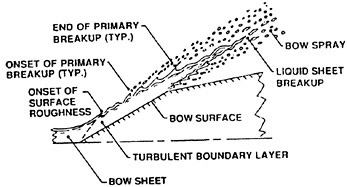
Fig. 1 Sketch of transitions of plane turbulent wall and free jets in still gases.
Turbulent primary breakup for round liquid jets has been recognized for some time (5–7). These and other early studies showed that liquid turbulence properties affected jet stability, the onset of breakup, and atomization quality after breakup (5–10). Finally, Hoyt and Taylor (11,12) provided considerable evidence that aerodynamic forces did not affect turbulent primary breakup in still air at NTP by showing that atomization properties for coflowing and counter-flowing round air/water jets at NTP were essentially the same.
Prompted by these observations, subsequent work by the present authors and their associates considered the properties of liquid surfaces and turbulent primary breakup for round turbulent-free jets (13–17) and plane turbulent wall jets (18,19) in still gases. These studies used pulsed shadowgraphy and holography to observe liquid surface properties and drop properties after turbulent primary breakup. The results showed that liquid surface and drop properties were related to liquid turbulence properties and yielded successful correlations based on phenomenological theories for several flow properties as follows: the onset of a roughened liquid surface for plane wall jets, the onset of drop breakup along the surface for both plane wall jets and round free jets, the end of drop breakup along the surface for round free jets, and the evolution of drop size and velocity
distributions along the liquid surface after turbulent primary breakup for both plane wall jets and round free jets. Merrill and Sarpkaya (20) have also considered the effect of wall roughness on the properties of turbulent primary breakup, showing that increased surface roughness enhances the turbulent primary breakup process.
The results of (13–19) demonstrate significant differences between the liquid surface properties and turbulent primary breakup processes of round turbulent-free jets. Thus, the objective of the present investigation was to extend past studies of turbulent primary breakup for round turbulent-free jets in still gases, using similar methods. The present measurements considered the variation of liquid surface velocities along the liquid surface, drop sizes produced at the onset of turbulent primary breakup along the liquid surface, and the evolution of mean drop sizes along the liquid surface as a function of distance from the jet exit. The experiments were limited to plane turbulent free water jets injected into still air at NTP, with the flows observed using pulsed shadowgraphy and holography. Phenomenological analysis was used to help interpret and correlate the measurements.
EXPERIMENTAL METHODS
Apparatus
The plane turbulent free jet test apparatus is illustrated in Fig. 2. All components of the apparatus in contact with the test liquid were constructed of type 304 stainless steel. The test liquid was placed within a cylindrical chamber that had an annular nozzle at the bottom. The inner diameter of the annular nozzle was roughly 50 mm, which yielded large aspect ratio annular jets (greater than 23:1) for present annulus widths in order to approximate plane free jets. The nozzle passages had smooth rounded entries with length/hydraulic diameter ratios greater than 40:1 to insure fully-developed turbulent flow at the jet exit (4,13). Injection was vertically downward with the core of the flow ventilated so that the annular sheet did not collapse.
Liquid was added to the test chamber through a port at the top. Premature liquid outflow was prevented by placing an annular cork in the nozzle exit. The liquid was then forced through the nozzle, ejecting the cork, by
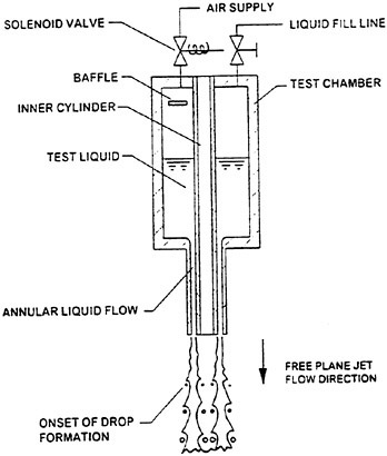
Fig. 2 Sketch of the plane turbulent free jet test apparatus.
admitting high-pressure air to the top of the test chamber through a solenoid-actuated valve. A baffle near the air inlet to the test chamber reduced mixing between the air and the test liquid. The solenoid was closed at the end of liquid delivery, allowing the test chamber to vent to the ambient pressure.
The high pressure air had a dewpoint less than 240 K and was stored in an accumulator on the upstream side of the solenoid valve. The accumulator had a volume of 0.12 m3 and provided air at pressures up to 1.9 MPa. The test chamber had an inside diameter of 190 mm and a length of 305 mm. The nozzle system provided annulus widths of 3.55 and 6.75 mm. Injected liquid was captured in a baffled tub. The entire test chamber and nozzle assembly could be moved vertically with an accuracy of 0.5 mm, using a linear bearing system in order to accommodate rigidly-mounted optical instrumentation.
Flow development times were 6–70 ms so that injection times of 100–400 ms yielded steady flow. Present optical instruments required less than 0.1 ms for triggering and data acquisition which did not impose any limitations on flow times. Jet velocities were calibrated in terms of the nozzle pressure drop by measuring liquid surface velocities from double-pulse shadowgraphs as discussed later.
Instrumentation
Instrumentation consisted of single- and double-pulse shadowgraphy and holography. Arrangements and methods were similar to earlier studies of turbulent primary breakup in this laboratory (15–19) and will only be described briefly. The light sources for both systems were frequency-doubled YAG lasers that could be controlled to provide pulse separations as small as 100 ns. Pulsed shadowgraphy was used in dilute regions of the flow (extending just beyond the onset of breakup), pulsed holography was used thereafter. Shadowgraphs were recorded using a 100×125 mm filter format with magnifications of 2–7. These photographs were obtained with an open camera shutter under darkroom conditions so that the 7 ns laser pulse duration controlled the exposure time. Use of different pulse strengths resolved directional ambiguity. The images were measured by mounting them on a two-dimensional traversing system having a 1 μm resolution which was viewed with a video camera and reduced using an image analysis program developed earlier (13).
An off-axis holographic arrangement was used with a 3:1 magnification of the object beam. This arrangement allowed drops having dimensions as small as 5 μm to be observed and as small as 10 μm to be measured with 10% accuracy. Analysis of hologram images was the same as the shadowgraphs except that the video camera could be traversed normal to the hologram with an accuracy of 5 μm.
Methods of data reduction were the same as Wu and coworkers (15–17) which should be consulted for details. Irregular drops were assumed to be ellipsoids and were assigned diameters equal to the diameter of a sphere having the same volume as the ellipsoid. Except for effects of this definition of drop diameters for irregular drops, which is difficult to quantify, experimental uncertainties of drop diameters are less than 10% for drop diameters larger than 10 μm, which comprised most of present measurements, increasing inversely proportional to the drop diameter for smaller sized drops. Measurements of SMD were obtained by summing over 40–400 objects at each condition to obtain experimental uncertainties (95% confidence) less than 15%, mainly dominated by sampling limitations.
Measurements of liquid surface velocities were based on the motion of particular points along ligaments while summing over 40–200 points to find average surface velocities with experimental uncertainties (95% confidence) less than 10%, mainly dominated by sampling limitations. Finally, measurements of the location of the onset of turbulent primary breakup were obtained as the average of 10 experiments with relatively large experimental uncertainties (95% confidence) of less than 30% due to sampling limitations.
Test Conditions
The tests involved water injected into still air. Past work has shown, however, that variations of liquid and gas properties are treated effectively by the dimensionless parameters used to summarize the present test results (15–19). The tests involved annulus hydraulic diameters of 7.1 and 13.5 mm, mean annulus velocities of 11.5–28.2 m/s, a local ambient pressure of roughly 100 kPa and a system temperatures of roughly 300 K. These conditions yielded ranges of experimental parameters, as follows: ρf/ρg=860, Refd=91,000–424,000, Wefd=13,000–151,000 and Ohfd=0.009–0.0012. This Reynolds number range is sufficiently high to insure fully-developed turbulent pipe flow at the jet exit, with the larger values approaching conditions representative of practical bow sheets. Similarly, the relatively small values of Ohfd imply relatively small direct effects of liquid viscosity on turbulent primary breakup, which also is representative of practical bow sheets.
RESULTS AND DISCUSSION
Flow Visualization
Consideration of the results will begin with visualization of the flow in order to provide insight about the general nature of the turbulent primary breakup processes. Shadowgraphs of the flow at various distances from the jet exit are illustrated in Fig. 3. These results are for an annulus width of 6.75 mm and a mean jet exit velocity of 15.8 m/s. The direction of motion of the liquid in the photographs is vertically downward, which corresponds to the orientation of the experiment. Four shadowgraphs are shown: one right at the jet exit which can be seen at the top of this shadowgraph and the other three centered at x/dh=8, 18 and 28. A 2.4 mm diameter pin is visible at the left of each shadowgraph to provide a distance reference. The liquid core is to the right in all four shadowgraphs.
The shadowgraphs of Fig. 3 illustrate a
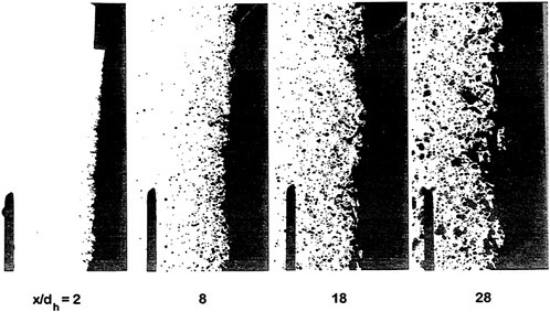
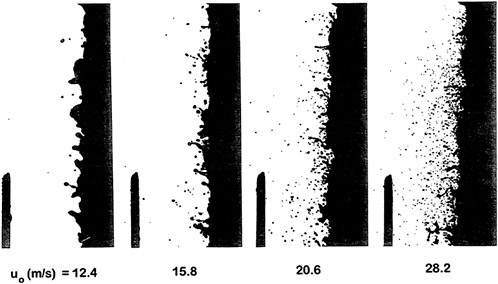
number of the general features of the liquid surface during turbulent primary breakup. First of all, the liquid surface becomes roughened or distorted very close to the jet exit. The size (both the diameter and length) of the surface roughness elements progressively increases with increasing distance from the jet exit; in fact, small scale distortions are not even superimposed on the large ligament structures seen at x/dh=28. Similar behavior has been observed in the past with the surface exhibiting fine-grained roughness near the jet exit and larger-scale irregularities appearing as distance from the jet exit is increased (13–17). This behavior is reasonable because small disturbances grow faster than large disturbances so they should appear first while small levels of turbulence production in the jet causes the turbulence to decay with the small scale portion of the spectrum disappearing first. The ligaments protruding from the liquid surface are randomly oriented rather than deflected toward the jet exit due to drag from the gas phase; this suggests small aerodynamic effects in agreement with past work at this density ratio (15–17). Finally, the mean position of the liquid surface bulges outward near the jet exit; past work suggests that this is caused by the evolution of the mean velocity profile in the liquid from turbulent pipe flow conditions at the jet exit to a nearly flat profile in the jet consistent with small effects of drag on the liquid surface (15).
Drop properties seen in Fig. 1 also are of interest. First of all, even though the liquid surface becomes roughened almost immediately, the first appearance of drops is deferred to x/dh≈3. This occurs because the surface energy required to form very small drops is not available at the smallest scales of the turbulence. After the onset of drop formation, however, drop diameters near the liquid surface progressively increase with increasing distance from the jet exit, in parallel with the scale of the ligaments and other surface distortions. This behavior is consistent with drops separating from attached ligaments by a Rayleigh breakup process, i.e., the ligaments act like liquid jets in the Rayleigh breakup regime.
Shadowgraphs of the flow near the liquid surface for various liquid velocities at a fixed distance from the jet exit are illustrated in Fig. 4. These results are for an annulus width of 6.75 mm with the shadowgraphs centered at x/dh=8. Injection is vertically downward, a 2.4 mm diameter reference pin appears at the left of each shadowgraph, and the liquid core is to the right of each photograph, similar to Fig. 3. Conditions at four mean jet exit velocities are shown: 12.4, 15.8, 20.6 and 28.2 m/s.
The effect of liquid velocity on the liquid surface properties observed in Fig. 4 is quite interesting. First of all, the length of the largest ligaments is seen to be relatively independent of liquid velocity. This behavior follows because eddy velocities scale with mean velocities for fully-developed turbulent flow. Thus, increasing mean velocities increases streamwise and lateral motion at the same rate so that distances traveled in the lateral direction when a given streamwise location is reached remain the same. In contrast, the smallest scale disturbances become progressively smaller as the liquid velocity increases because the kinetic energy available to distort the surface at large wave numbers increases as the velocity, and thus, the Reynolds number of the flow increases. The net effect is similar to turbulent jet mixing processes where increasing jet velocities (Reynolds numbers) do not affect the global mixing process of the flow even though fine scale mixing is increased (21–23).
Similar to Fig. 3, drop properties after primary breakup in Fig. 4 generally are related to the properties of the distortion of the liquid surface. Thus, drop sizes at the location shown tend to decrease similar to the reduced diameters of the ligaments, as the liquid velocity increases. This causes an increase in drop number density near the surface with increasing velocity because the drop diameters decrease. Measurements of liquid volume fractions in similar flows, however, suggest that they are not correspondingly influenced by liquid jet velocity (13,14). Such behavior is quite reasonable based on the earlier discussion because the global mixing rates do not change rapidly due to jet velocity variations.
Liquid Surface Velocities
The present plane turbulent free jets are injected from a passage into a uniform pressure field containing still air. Thus, liquid surface velocities should increase at first as the retarding effect of the passage wall decays away near the jet exit before finally decreasing due to effects of flow resistance at the gas/liquid interface. Thus, mean liquid surface velocities were measured as a function of distance along the surface, in order to establish jet flow properties.
Typical measurements of free jet mean
surface velocities in the streamwise direction are plotted for various jet hydraulic diameters and velocities in Fig. 5. Liquid surface velocities are normalized by the mean jet exit velocity while the streamwise distance is normalized by the radial integral length scale. Similar to past work, the streamwise integral length scale is taken to be 4Λ while Λ=dh/8, based on Laufer’s measurements of the properties of fully-developed turbulent pipe flow, see Hinze (22) and references cited therein. Results for various test conditions plot in the same way when normalized in this manner. Surface velocities increase near the jet exit, approaching ūS/uo≈1at x/Λ=200, and then remain relatively constant for the rest of the test range (x/Λ<800). This behavior is in good agreement with earlier observations of velocities near the surface of round turbulent free jets (15). In contrast, plane turbulent wall jets exhibit a significant velocity decay for similar streamwise distance (18,19). These differences highlight the relatively weak effects of drag at the gas/liquid interface for free jets, compared to the solid surface of a plane turbulent wall jet.
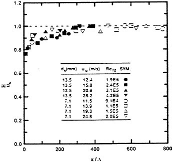
Fig. 5 Mean liquid surface velocities as a function of streamwise distance along plane turbulent free jets.
Drop Size Distributions
Drop size distributions have not been measured for the present turbulent primary breakup process. Past work, however, has shown good agreement between the universal root normal distribution of Simmons (24), with MMD/SMD=1.2, and measured drop size distributions for a variety of primary and secondary breakup processes (13–19,25,26). Assuming that this size distribution is appropriate for the present turbulent primary breakup process, specification of the one moment of this two-moment distribution function implies that the drop size distribution is known. Thus, drop sizes will be summarized in terms of the SMD alone, in the following.
Onset of Primary Breakup
The properties of the onset of primary breakup for plane turbulent free jets were analyzed in the same manner as earlier studies of primary breakup of round turbulent free jets (15–17) and for plane turbulent wall jets (18,19). Thus drops formed at the onset of turbulent primary breakup are the smallest drops that can be formed by this mechanism. This condition was found by equating the kinetic energy (relative to its surroundings) of an eddy of a particular characteristic size, to the surface energy required to form a drop of corresponding size. Both drop and eddy sizes were assumed to be in the inertial range of the turbulence spectrum which was appropriate for present test conditions, see (17) for consideration of drop formation outside the inertial range of the turbulence. Within the inertial range characteristic eddy sizes and velocities are related in a simple way as discussed by Tennekes and Lumley (23). Finally, the SMD resulting from turbulent primary breakup was associated with the characteristic eddy size to yield the following expression for the SMD at the onset of turbulent primary breakup (15–19):
(1)
where Csi is an empirical constant on the order of unity involving the various proportionality constants. Given that ![]() is also a constant for fully-developed turbulent pipe flow, SMDi/Λ should only be a function of
is also a constant for fully-developed turbulent pipe flow, SMDi/Λ should only be a function of ![]() for present test conditions.
for present test conditions.
Present measurements of SMDi are plotted as suggested by (1) in Fig. 6. Also plotted on the figure are the measurements and correlations of Wu and Faeth (17) for round turbulent free jets and the correlation of Dai et al. (18,19) for plane turbulent wall jets. The present measurements for plane free jets agree within experimental uncertainties with the earlier measurements for round free jets suggesting that use of the hydraulic diameter correctly approximates the effect of the different configurations of these two flows. Thus, the
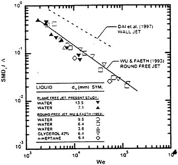
correlation of (17) provides a good fit of both sets of measurements, as follows:
(2)
The standard deviations of the coefficient and power of (2) are 10% and 7%, respectively, and the correlation coefficient of the fit is 0.79. The reduction of the power of ![]() from −3/5 in (1) to −0.74 in (2) is statistically significant but is not large in view of the approximations used to find (1) and present experimental uncertainties. The coefficient of (2) is large but this can be anticipated from (1) because
from −3/5 in (1) to −0.74 in (2) is statistically significant but is not large in view of the approximations used to find (1) and present experimental uncertainties. The coefficient of (2) is large but this can be anticipated from (1) because ![]() is large; thus, Csi is on the order of unity as expected. The correlation of Dai et al. (18,19) for plane wall jets yields values of SMDi that are of the same order of magnitude but larger than the results for free jets at comparable conditions. Such differences are not unreasonable, however, when it is recalled that free jets represent slowly decaying flows with turbulence properties dominated by near solid surface conditions at onset near the jet exit, while the wall jets represent developing flows dominated by conditions far from the solid surface.
is large; thus, Csi is on the order of unity as expected. The correlation of Dai et al. (18,19) for plane wall jets yields values of SMDi that are of the same order of magnitude but larger than the results for free jets at comparable conditions. Such differences are not unreasonable, however, when it is recalled that free jets represent slowly decaying flows with turbulence properties dominated by near solid surface conditions at onset near the jet exit, while the wall jets represent developing flows dominated by conditions far from the solid surface.
An expression for the distance from the jet exit where turbulent primary breakup is initiated is also developed following earlier studies of turbulent primary breakup (15–19). It is assumed that the initial drop-forming eddy convects along the surface with the streamwise velocity ūo for the time required far eddy having the appropriate characteristic size to form a drop. Based on past success of this approach, the breakup time taken to be the time required for Rayleigh breakup of a ligament having a diameter equal to the characteristic eddy from Weber (27) while ignoring a viscous term that might become important at large jet Ohnesorge numbers. Fixing the characteristic size from the SMDi of (1) then yields the following expression for the location of the onset of breakup (15–19):
(3)
where Cxi is an empirical constant on the order of unity involving the various proportionality constants for fully-developed turbulent pipe flow.
Present measurements of xi are plotted as suggested by (3) in Fig. 7. Also plotted on the figure are the measurements and correlation of Wu and Faeth (17) for round turbulent free jets and the correlation of Dai et al. (18–19) for plane turbulent wall jets. The present measurements for plane free jets agrees within experimental uncertainties with the earlier measurements for round free jets; this behavior also supports the use of hydraulic diameters to obtain a combined
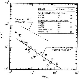
correlation for the two flows. Thus, the correlation of (15) provides a good fit of both sets of measurements, as follows:
(4)
The standard deviations of the coefficient and power of (4) are 10% and 12%, respectively and the correlation coefficient of the fit is 0.96. As before, the power of ![]() for the correlation of the data is not −0.4 as suggested by (3). This reduction of the power of
for the correlation of the data is not −0.4 as suggested by (3). This reduction of the power of ![]() is statistically significant but is also not large in view of the approximations used to find (3) and the relatively large experimental uncertainties of the xi. Finally, the large value of the constant in (4) can be anticipated from the large values of
is statistically significant but is also not large in view of the approximations used to find (3) and the relatively large experimental uncertainties of the xi. Finally, the large value of the constant in (4) can be anticipated from the large values of ![]() in (3), while the value of Cxi is on the order of unity as expected.
in (3), while the value of Cxi is on the order of unity as expected.
Drop Sizes Along Surface
The approach used to find the variation of SMD with distance from the jet exit was similar to the method used to find xi (15–19). It was assumed that drops near the liquid surface formed recently due to turbulent primary breakup because they have relatively large radial velocities (15). The following assumptions were also made: the SMD is dominated by the largest drop that can be formed at a particular position, an eddy of this characteristic size forms a drop by Rayleigh breakup while effects of liquid viscosity on breakup are small, and the SMD is proportional to the characteristic eddy size. Then, following a procedure similar to the derivation of (3) yields the following expression for the variation of SMD with distance from the jet exit:
(5)
where Csx is a constant of proportionality that should be of order unity.
Present measurements of SMD for plane turbulent free jets are plotted in terms of the variables of (5) in Fig. 8, along with best fit correlations of the round turbulent-free jet measurements of Wu et al. (15), plane turbulent wall jet measurements of Dai et al. (18,19) and the present measurements. The correlations for the three flows are well within the scatter expected based on experimental uncertainties. The best fit correlation of the present measurements is as follows:
(6)
The standard deviations of the coefficient and power of (6) are 24% and 6%, respectively, and the correlation coefficient of the fit is 0.98. The differences between the power of the best fit of the data, 0.50, and the power predicted by the simplified theoretical results of (5), 0.67, is statistically significant. The differences between these powers are not large, however, in view of the approximations of the simplified analysis. Finally, the coefficient of (6), Csx, is on the order of unity as expected because there is no term proportional to ![]() which becomes large in this case. Taken together, the fact that Csi, Cxi and Csx all had reasonable magnitudes, on the order of unity, while the coefficients of (2), (4) and (6) had values properly associated with the ratio of
which becomes large in this case. Taken together, the fact that Csi, Cxi and Csx all had reasonable magnitudes, on the order of unity, while the coefficients of (2), (4) and (6) had values properly associated with the ratio of ![]() to some power, which can generate large numbers, helps to support the physical ideas used to develop (1)–(6).
to some power, which can generate large numbers, helps to support the physical ideas used to develop (1)–(6).
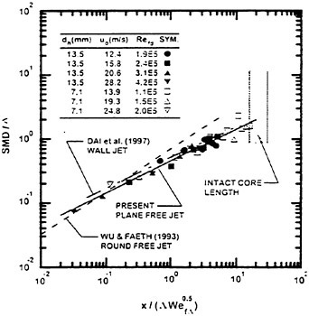
Fig. 8 SMD after turbulent primary breakup as a function of Weber number: plane turbulent wall jets results from Dai et al. (19), round turbulent free jet results from Wu and Faeth (16) and plane turbulent free jet results from the present study. Intact core length correlation from Grant and Middleman (8).
Increasing distance will eventually yield a condition where the SMD approaches the liquid jet diameter according to (5). It is interesting to note that this condition corresponds to a correlation for liquid core length (or jet breakup length) from Grant and Middleman (8), as follows:
(7)
This expression appears as a band in Fig. 8, for the present Wefd range (note that Λ=dh/8 has been used to plot (7) in Fig. 8, as before). It is interesting to note that this region corresponds to conditions where present results provide SMD/Λ on the order of unity which provides a reasonable physical mechanism for ending the length of the liquid core, i.e., drop sizes after turbulent primary breakup are comparable to the liquid core size at this condition.
CONCLUSIONS
The velocities of the liquid surface and of drop sizes after turbulent primary breakup along the liquid surface were measured for plane turbulent free jets in still air at normal temperature and pressure. The experiments were limited to water for the following test range: ρf/ρg≈860, Refd=91,000–424,000, Wefd=13,000–151,000 and Ohfd=0.0009–0.0012, the last implying conditions where direct effects of liquid viscosity are small. The major conclusions of the study are as follows:
-
The presence of roughness at the liquid surface, and turbulent primary breakup along the liquid surface, was caused by turbulence developed within the injector passage while direct effects of aerodynamic forces at the liquid surface were small, for present conditions.
-
Drop sizes at the onset of turbulent primary breakup along the liquid surface could be correlated by equating the surface energy required to form a drop to the kinetic energy of an eddy of corresponding size within the inertial range of the turbulence spectrum. Onset of turbulent primary breakup could also be controlled by either the smallest (Kolmogorov) or the largest turbulence scales in the liquid but such conditions were not observed during the present investigation.
-
The position of the onset of turbulent primary breakup along the liquid surface could be correlated by considering the distance convected at the mean velocity of the wall jet for the residence time needed to initiate Rayleigh breakup of the ligaments protruding from the liquid surface that are associated with the formation of drops of similar size at the onset of breakup.
-
Drop sizes after turbulent primary breakup progressively increased with increasing distance along the surface at a given jet velocity, and progressively decreased with increased jet velocity at a given position along the surface. The variation of drop sizes with distance satisfied the same relationship as the onset of turbulent primary breakup and could be explained by associating the SMD with the largest drops that had sufficient residence time in the flow to be formed at a particular location due to Rayleigh breakup of protruding ligaments of similar size.
-
Extrapolating the variation of drop sizes with streamwise distance suggests that the SMD after turbulent primary breakup becomes comparable to the width of the liquid column for conditions where the end of the liquid core is approached (based on the Grant and Middleman (8) correlation of liquid core length).
-
The conventional use of hydraulic diameters yields correlations for the SMD and location at the onset of turbulent primary breakup, and for the variation of SMD after turbulent primary breakup as a function of distance along the surface, that are identical (within experimental uncertainties) for round and plane free turbulent jets. In contrast, onset of turbulent primary breakup for plane wall jets is deferred to larger drop sizes and distances from the jet exit compared to the free jets, although the variation of SMD with distance along the surface is similar for all three flows. It is thought that the difference of onset properties comes about because onset of turbulent primary breakup involves small turbulence scales near surfaces for the free jets in contrast to large turbulence scales far from surfaces for the wall jets.
-
Streamwise liquid surface velocities remained nearly constant (within 10%) over most of the liquid surface for the range considered during present test conditions (50<x/Λ<800) which simplifies interpretation of turbulent primary breakup properties. Surface velocities decrease near the jet exit due to the retarding effect of the jet passage walls on liquid motion.
Present results are limited to liquids having moderate viscosities at conditions with fully-developed turbulence in the liquid, with drop sizes after turbulent primary breakup
comparable to eddy sizes in the inertial range of the turbulence, with liquid surface breakup not too near the end of the all-liquid column and where aerodynamic effects on turbulent primary breakup are not important. Addressing these limitations merits further attention due to the importance of turbulent primary breakup to the properties of natural, ship-generated and industrial sprays.
ACKNOWLEDGMENTS
This research was sponsored by the Office of Naval Research Grant No. N00014–95–1–0234 under the technical management of E.P. Rood. Initial development of research facilities for this study was carried out under Air Force Office of Scientific Research Grant No. AFOSR F49620–95–1–0364 under the technical management of J.M.Tishkoff. The help of W.-H.Chou during the early phases of the study is gratefully acknowledged.
REFERENCES
1. Gad-el-Hak, M., “Measurements of Turbulence and Wave Statistics in Wind-Waves.” International Symposium on Hydrodynamics in Ocean Engineering, The Norwegian Institute of Technology, Oslo, Norway, 1981, pp. 403–417.
2. Townson, J.M., Free-Surface Hydraulics, 1st ed., Unwin Hyman, London, 1988, Chapt. 6.
3. Ervine, D.A., and Falvey, H.T., “Behavior of Turbulent Water Jets in the Atmosphere and in Plunge Pools,” Proc. Inst. Civ. Eng., Pt. 2, Vol. 83, Mar. 1987, pp. 295–314.
4. Wu, P.-K., Miranda, R.F., and Faeth, G.M., “Effects of Initial Flow Conditions on Primary Breakup of Nonturbulent and Turbulent Round Liquid Jets,” Atomization and Sprays, Vol. 5, No. 2, 1995, pp. 175–196.
5. De Juhasz, K.J., Zahn, O.F., Jr., and Schweitzer, P.H., “On the Formation and Dispersion of Oil Sprays,” Bulletin No. 40, Engineering Experimental Station, Pennsylvania State University, University Park, PA, 1932, pp. 63–68.
6. Lee, D.W., and Spencer, R.C., “Preliminary Photomicrographic Studies of Fuel Sprays,” NACA Tech. Note 424, Washington, D.C., 1933.
7. Lee, D.W., and Spencer, R.C., “Photomicrographic Studies of Fuel Sprays,” NACA Tech. Note 454, Washington, D.C., 1933.
8. Grant, R.P., and Middleman, S., “Newtonian Jet Stability,” AIChE Journal, Vol. 12, No. 4, 1966, pp. 669–678.
9. Phinney, R.E., “The Breakup of a Turbulent Jet in a Gaseous Atmosphere,” Journal of Fluid Mechanics, Vol. 60, Pt. 4, 1973, pp. 689–701.
10. McCarthy, M.J., and Malloy, N.A., “Review of Stability of Liquid Jets and the Influence of Nozzle Design,” Chemical Engineering Journal, Vol. 7, No. 1, 1974, pp. 1–20.
11. Hoyt, J.W., and Taylor, J.J., “Waves on Water Jets,” Journal of Fluid Mechanics, Vol. 88, Pt. 1, 1977, pp. 119–123.
12. Hoyt, J.W., and Taylor, J.J., “Turbulence Structure in a Water Jet Discharging in Air,” Physics of Fluids, Vol. 20, Pt. II, No. 10, 1977, pp. S253–S257.
13. Ruff, G.A., Wu, P.-K., Bernal, L.P., and Faeth, G.M. “Continuous- and Dispersed-Phase Structure of Dense Non-evaporating Pressure-Atomized Sprays,” Journal of Propulsion and Power, Vol. 8, No. 2, 1992, pp. 280–289.
14. Tseng, L.-K., Ruff, G.A., and Faeth, G.M., “Effects of Gas Density on the Structure of Liquid Jets in Still Gases,” AIAA Journal, Vol. 30, No. 6, 1992, pp. 1537–1544.
15. Wu, P.-K., Tseng, L.-K., and Faeth, G.M., “Primary Breakup in Gas/Liquid Mixing Layers for Turbulent Liquids,” Atomization and Sprays, Vol. 2, No. 3, 1992, pp. 295–317.
16. Wu, P.-K., and Faeth, G.M. “Aerodynamic Effects on Primary Breakup of Turbulent Liquids,” Atomization and Sprays, Vol. 3, No. 3, 1993, pp. 265–289.
17. Wu, P.-K., and Faeth, G.M., “Onset and End of Drop Formation Along the Surface of Turbulent Liquid Jets in Still Gases,” Physics of Fluids A, Vol. 7, No. 11, 1995, pp. 2915–2917.
18. Dai, Ζ., Hsiang, L.-P., and Faeth, G.M., “Spray Formation at the Free Surface of Turbulent Bow Sheets,” Proceedings of the Twenty-First Symposium on Naval Hydrodynamics, National Academy Press, Washington, D.C., 1997, pp. 490–505.
19. Dai, Z., Chou, W.-H., and Faeth, G.M., “Drop Formation Due to Turbulent Primary Breakup at the Free Surface of Plane Liquid Wall Jets,” Physics of Fluids, in press.
20. Merrill, C.F., and Sarpkaya, T., “Spray Formation at the Free Surface of a Liquid Wall Jets,” AIAA Paper No. 98–0442, 1998.
21. Schlichting, H., Boundary Layer Theory, 7th ed., McGraw-Hill, New York, 1979, p. 599.
22. Hinze, J.O., Turbulence, 2nd Ed., McGraw-Hill, New York, 1975, p. 427 and pp. 724–734.
23. Tennekes, H., and Lumley, J.L., A First Course in Turbulence, MIT Press, Cambridge, MA, 1972, pp. 248–286.
24. Simmons, H.C., “The Correlation of Drop-Size Distributions in Fuel Nozzle Sprays,” J. Engr. for Power, Vol. 99, No. 1, 1977, pp. 309–319.
25. Hsiang, L.-P., and Faeth, G.M., “Near-Limit Drop Deformation and Secondary Breakup,” Int. J. Multiphase Flow, Vol. 18, No. 5, 1992, pp. 635–652.
26. Hsiang, L.-P., and Faeth, G.M., “Drop Properties After Secondary Breakup,” Int. J. Multiphase Flow, Vol. 19, No. 5, 1993, pp. 721–735.
27. Weber, C., “Zum Zerfall eines Flussigkeitsstrahles,” Z. Angewesen. Math. Mech., Vol. 2, 1931, pp. 136–141.
DISCUSSION
T.Sarpkaya
Naval Postgraduate School, USA
I have been very interested with the authors’ presentation and their related contributions, cited in their references, because of our own work on spray formation at the free surface of plane liquid wall jets. I would, therefore, like to raise the following questions:
-
In this as well as in their related papers the authors refer to “plane turbulent free jets,” “round turbulent free jets,” and “plane turbulent wall jets.” If I am not mistaken, none of their papers dealt with “plane turbulent jets” with or without a wall. In fact, their jets are axisymmetric, with or without an axisymmetric cylinder at the center serving as a wall. It seems to me that “annular liquid wall jets about axisymmetric rods” and “annular free liquid sheets” would be more suitable terms for their experiments. Is the use of hydraulic radius (as in subcritical deep channel flows with reasonable cross sections) sufficient to assume that axisymmetric, highly disturbed, turbulent, supercritical jets behave like their plane-wall counterparts (e.g., bow sheets)?
-
Authors have found best-fit correlations for every major parameter (e.g., SMD, location of the onset of breakup) in terms of the Weber number (to some power), multiplied by a constant. In doing so, they have invoked the information gathered from fully-developed turbulent pipe flows. Considering the fact that a thin sheet of high-speed supercritical jet is very much unlike a turbulent pipe flow (large structures of the free surface are affected by and affect the entire flow structure), how could one justify the use of pipe-flow concepts? What physics can one deduce from the said correlations?
-
Is it not true that the development of the mean liquid surface velocities depends on the length of the “inner cylinder” and the length of the exit pipe (Figs. 2 and 5)? What is the effect of the change of the thickness of the jet in their free- as well as wall-jets?
-
In wall jets of the type used by the authors could one examine the effect of wall roughness in view of the fact that ship bows are always rough? How do the present results relate to the behavior of bow sheets?
After considerable thought on sprays, I have succeeded in convincing myself that I do not really understand the role of the correlations offered by the authors either in understanding the physics of the phenomenon or in making predictions for technological applications. I am sure the authors’ words of wisdom, based on their many years of experience, will be enlightening to all interested in spray phenomena.
AUTHORS’ REPLY
The following replies are numbered to correspond to Professor Sarpkaya’s discussion:
-
Research experiments generally use one of two major strategies to approximate turbulent plane jets, as follows: (1) large aspect ratio plane slot jets, either with or without side walls to help promote two dimensional flow in the mean; and (2) large aspect ratio annular slot jets. Annular slot jets have been used during our studies because they offer a number of advantages, as follows: the geometry is well defined with no uncertainties about effects along side walls, or the edges of the flow, large aspect ratio annular flows are formally two dimensional with no mean crossflows due to edge effects, and the round geometry of annular flows improves optical access for observations near the liquid surface of dense sprays compared to penetrating dense sprays for long distances as required by large aspect ratio plane jets. Present measurements involved the use of two jet exit annulus widths, 3.55 and 6.75 mm with an inside annulus diameter of 50 mm; this provided aspect ratios of 44 and 23, which are relatively large. In addition, our measurements of various flow properties in Figs. 5–8 show similar results for the two slot widths which does not suggest significant effects of curvature. More importantly, present results for large aspect ratio nearly plane jets are in excellent agreement with earlier results for round jets due to Wu and Faeth (16). see Figs. 6–8, after using standard concepts of hydraulic diameters to provide unified correlations of the turbulent flows. Furthermore, Dai et al. (18,19) observe similar capabilities for hydraulic diameters to provide unified correlations of the turbulent primary breakup properties of wall jets having a wide range of aspect ratios. Taken together, these findings do not suggest diffi-
-
culties with effects of small degrees of curvature used during the experiments.
-
The phenomenological analyses that were used to help interpret and correlate the present measurements only require relatively robust properties that are present in all turbulent flows. This includes the existence of an inertial range of the turbulence spectrum in order to relate eddy sizes and velocities, the presence of large (integral) scales to define the small wave number limit of the inertial range, and the presence of small (Kolmogrov) scales to define the large wave number limit of the inertial range. The resulting correlations for the properties of onset of turbulent primary breakup, and for the variation of drop sizes after turbulent primary breakup with distance along the jet, do not indicate any major difficulties with present hypotheses about turbulence properties: the correlations of the various properties are quite good with correlation coefficients near unity; the measured powers of dimensionless parameters in the various correlations are in reasonable agreement with expectations based on phenomenological analysis; the empirical coefficients Csi, Cxi and Csx all are on the order of unity as expected; and values of coefficients properly assume large values due to the presence of terms involving
 as suggested by the phenomenological analyses. These properties now have been observed during turbulent primary breakup for plane and round free jets, and for plane wall jets; see (15–19) and the present study.
 -
Liquid velocities within the test chamber are small; therefore, jet exit conditions are established in the annular passage at the exit of this chamber. This passage was designed so that its length/hydraulic-diameter ratios are greater than 40:1, which insures fully-developed turbulent flow at the jet exit for the rather large Reynolds number (Refd≥91,000) used during the present experiments; see Wu et al. (4) and references cited therein. For such conditions, the effect of increased annular passage lengths is small. Finally, measurements for two different slot widths are discussed in the paper, with results for these two different conditions correlated quite well using hydraulic diameter concepts, as noted earlier.
-
The relative roughness of bow sheets is affected by operating conditions, hull design, maintenance, fouling and damage so a range of conditions must eventually be understood. Thus, flows along smooth surfaces provide a logical starting point for the present studies, particularly in view of the fact that current detailed models of flows along ship surfaces generally are limited to consideration of smooth surfaces.
-
The information provided by the correlations found during the present and past studies includes the onset and end of turbulent primary breakup along surfaces, drop size, and velocity distributions after turbulent primary breakup, and the variation of drop sizes and velocities along the liquid surface. This information is crucial for understanding and modeling the structure, and the optical and radar scattering properties, of the dispersed flow region adjacent to the bow sheet, which is of interest for practical applications. In particular, turbulent primary breakup controls the overall mixing rates of gas and liquid and sets boundary conditions for analysis of spray processes within the dispersed flow region; see Faeth et al. (28) and references cited therein for reviews of current methods of analyzing dense sprays typical of the dispersed flows associated with bow sprays.
References
28. Faeth, G.M., Hsiang, L.-P., and Wu, P.-K., “Structure and Breakup Properties of Sprays,” Int. J. Multiphase Flow, Vol. 21, Suppl., 1995, pp. 99–127.
Some Structural Features of Pressure-Driven Three-Dimensional Turbulent Boundary Layers from Experiments for 500≤Reθ≤23000
R.Simpson, M.Ölçmen
(Virginia Polytechnic Institute and State University, USA)
Abstract
Pressure-driven three-dimensional turbulent boundary layers are commonplace in hydrodynamic flows. A variety of experiments over a wide range of momentum thickness Reynolds numbers Reθ has revealed some generalizations about the behavior of three-dimensional turbulent boundary layers. These include the anisotropic nature of the eddy viscosity and the lags between the mean flow gradients and the turbulence. The v’ rms normal-to-wall velocity fluctuation appears to be an important velocity scale. The parameters ![]() and
and ![]() are independent of rotation about the normal to wall axis and have nearly universal relationships in the outer region of many non-equilibrium 3D boundary layers. Comparisons of some second-order turbulence models with results deduced from detailed measurements indicate that better modeling of pressure and turbulence diffusion and pressure/rate-of-strain terms is needed, especially near the wall. Some work underway is providing v spatial correlation data that are needed for estimating the pressure fluctuation related terms.
are independent of rotation about the normal to wall axis and have nearly universal relationships in the outer region of many non-equilibrium 3D boundary layers. Comparisons of some second-order turbulence models with results deduced from detailed measurements indicate that better modeling of pressure and turbulence diffusion and pressure/rate-of-strain terms is needed, especially near the wall. Some work underway is providing v spatial correlation data that are needed for estimating the pressure fluctuation related terms.
Introduction
Three-dimensional pressure-driven turbulent boundary layers (3DTBL) occur in many practical hydrodynamic cases, which are mostly non-equilibrium flows. The imposed spanwise pressure gradient causes a change in direction of the flow as a function of distance from the wall. The purpose of this article is to give some features of the structure of such flows as revealed from many recent experiments, which can increase the understanding and improve the modeling of these flows.
Simpson (1996) presented a perspective on 3DTBL behavior and reviewed many related referenced works. Here we will summarize first the key insights and conclusions from that work and augment them with some new observations. While results from many other flow cases will be included, the principal example geometry will be the flat-wind-tunnel-wall 3-D turbulent boundary layer (approach momentum thickness Reynolds numbers of Reθ=5940 and very recently 23000) and the horseshoe-vortex flow around the junction with a 3:2 elliptic nose, NACA 0020 tail appendage (Figure 1), which was experimentally examined by the authors. These wind tunnel results are compared with some recent water tunnel results for this geometry at much lower Reθ values.
Using these and other experimental data sets, the strong relationship between the normal to the wall rms fluctuation v’ and the shearing stress magnitude will be discussed, along with other observed relationships among important velocity fluctuation triple products in some stress transport equations. A summary will be given of comparisons between some second-order modeling equations with experimental results. Finally, some comments will be made on needed and future work.
Summary of Some Previous Insights
Simpson (1996) and Johnston and Flack (1996) implicitly show that many recently revealed features of 3DTBLs are due to the use of three-velocity-component laser-Doppler anemometry. In our work a specially-designed fine-spatial-resolution (30 μm spherical measurement volume diameter) fiber-optic laser-Doppler velocimeter (LDV) (5-velocity-component) is used for pointwise and two-point spatial correlation measurements as close to the wall as y+=3 (Ölçmen and Simpson, 1995b). Although one should be able to infer the wall shearing stress τw from the nearest-wall LDV velocity profile, Johnston and Flack suggest that there is a continuing need for improved direct measurement of τw.
Examination of a number of data sets shows that no universal law-of-the-wall mean-velocity profile exists. Local near-wall equilibrium along some flows cause the mean velocity profiles to be self-similar in wall co-ordinates, but without a universal mean-velocity profile law. A law-of-the-wall semi-logarithmic profile with universal constants only seems to exist for the beginning stages of 3-D flow. Without a relationship with universal constants, the law-of-the-wall concept loses much of its usefulness.
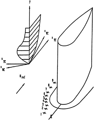
Figure 1. Schematic view of the appendage and measurement locations; descriptions of tunnel co-ordinates ()TC and wall co-ordinates ()WC.
The eddy viscosity is highly anisotropic in 3-D flows. Algebraic turbulence models that relate shear stresses to mean velocity gradients through eddy viscosities and mixing lengths continue to be widely used in aerodynamic and hydrodynamic calculations, largely because of their relative simplicity compared to other models and the collective experience of users of these models. These models are crude approximations to the flow physics and are not robust for strongly 3-D cases, such as separated flows. Accelerating portions of 3D flows with weak crossflows may be adequately calculated with this approach, but adverse pressure gradient flows are not well calculated. The observed reduction in eddy viscosity magnitude, as compared to algebraic eddy viscosity models, is due to non-equilibrium lags in the turbulence structure, which usually accompany strong adverse pressure gradients, even in 2D cases.
The mean turbulent shearing stresses generally lag the mean velocity gradient direction, so that an isotropic eddy viscosity turbulence model cannot reflect the correct physics of the stress-producing structures. There appears to be a reduction in the correlation between the shearing stress and the turbulent kinetic energy due to the different histories of the outer layer and inner layer flow structures—they come from different upstream directions (Figure 2). In the wall shear-stress co-ordinates, there appears to be a nearest-wall region in which the mean flow direction does not change much with the distance from the wall. However, the turbulent shear-stress direction is generally different from this direction and the mean-velocity gradient direction.
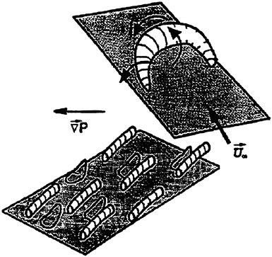
Figure 2. Coherent structures in a skewed 3-D turbulent boundary layer. Outer layer “croissant-shaped” structures that entrain free-stream fluid move in different directions than the near-wall quasi-streamwise vortices.
The eddy viscosity for the spanwise direction νz is not a constant factor Nc times the streamwise eddy viscosity νx and depends upon the co-ordinate system. Nc appears to be about constant in the outer layer but varies much near the wall. In more detail than presented here, Simpson (1996) discusses the data and suggests that Nc=0.6 in a wall-shearing-stress co-ordinate system or local streamline co-ordinate system is a prescription for crudely accounting for anisotropy in eddy viscosity calculation methods in many flows. This prescription of co-ordinate system forces the spanwise shearing stress near the wall to approach zero either with a constant or varying Nc since the crossflow velocity gradient ∂W/∂y is zero at the wall. While a number of experiments have
about this value of Nc, other flows examined by Ciochetto and Simpson (1997) have Nc values away from the wall that are closer to unity, e.g., Pompeo et al. (1992, 1993) and Schwarz and Bradshaw (1992, 1993).
This prescription can also be justified from a physical viewpoint; the relatively large wall-region turbulent shear stresses control the flow more than the outer layer stresses and need to be more accurately modeled. The nearest-wall flow seems to approximate a mean 2-D flow. The wall-stress co-ordinates are more closely aligned than local free-stream co-ordinates with the mean shear stress direction (SSA) in this region. Therefore, near-wall estimates of νx in WC will be similar to mean 2-D cases and errors in νz will have less impact on the calculated total Reynolds shear stress.
Some Features of an Example Reynolds-averaged 3-D Flowfield Over a Wide Range of Reynolds Numbers
The well-documented wing/body junction low-speed flow (approach flow Reθ=5940) of Ölçmen and Simpson (1995a, 1996a) can be used as a computational test case of turbulence models, as pointed out by Rizzi and Vos (1998). The mean 2-D upstream flow develops into a non-equilibrium 3-D flow and then relaxes back toward a mean 2-D flow far downstream. In addition to measurements along the path shown in Figure 3(a), which is outside the region near the wing where large mean flow streamwise vortices are dominant, the mean flowfield and Reynolds stresses have been obtained over large regions of this geometry: (1) the nose separated flow and juncture vortex around the side of the wing, which is briefly discussed below (Devenport and Simpson, 1990a, b, c; Ölçmen and Simpson, 1997b); (2) the mean 2-D flow entrance conditions (Ölçmen and Simpson, 1990, 1995a); and (3) the downstream wake region (Fleming et al., 1991). Skin friction magnitude |τw/ρ|=Uτ2 and direction were directly measured using oil-film interferometry (Ailinger and Simpson, 1990). In addition, convective heat-transfer and the temperature field have been measured for this flowfield (Lewis et al., 1993, 1996, 1998).
Figure 3(b) shows mean velocity profiles at these stations in local wall shear stress coordinates and wall velocity Uτ and length v/Uτ scales. In upstream flow direction or wind tunnel coordinates (Simpson 1996), the streamwise wind tunnel mean flow velocity U first slightly decelerates due to the adverse pressure gradient and then accelerates around the wing, while the crossflow W magnitude increases along the flow. The maximum W magnitude in tunnel coordinates is located progressively further from the wall. In the outer region of a pressure-driven flow the Reynolds shearing stresses persist with the upstream 2DTBL magnitude and direction until the 3-D effects propagate to that location away from the wall. It appears that transport equations are needed to account for this nature of the lag within the flow.
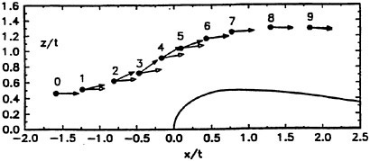
Figure 3(a) Appendage shape and Stations 1–9 measurement locations. Full arrows are in wall-stress direction. Empty arrows are in free-stream direction.
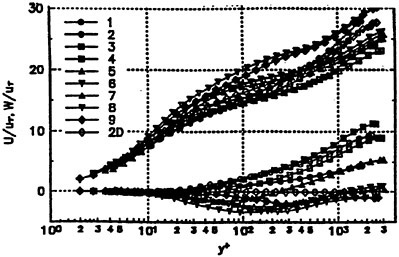
Figure 3(b). U/Uτ, and W/Uτ mean velocity profiles for the Reθ=5940 flow in wall-stress co-ordinates. The uncertainties are on the order of the symbol size.
Using multiple probes in the wind tunnel flow, Ha and Simpson (1993) found that the coherency of larger-scaled structures appear to be reduced by the effects of three-dimensionality. This length scale reduction occurs with the growth of 3-D turbulence effects near the wall that are unrelated to the outer region flow that originated from another direction in the upstream flow (Figure 2). Length scales in the outer region showed no change along the flow, indicating strong persistence of the coherency of outer region structures along the local free-stream direction. In the low Reynolds number cases, length scale results from autocorrelations revealed 50% shorter integral length scales for the 3-D flow as compared to a 2-D flow, which is consistent with the higher Reynolds number wind tunnel results.
The skewing angle of the coherent structures closely follows the local mean velocity angle especially in the inner region, indicating that the coherent
structures are convected in the mean flow direction. In the outer layer at this location, equally coherent motions occur over a wider angular range between the far upstream 2-D flow direction and the local flow direction. This indicates that the direction of the far upstream outer region coherent motions lags for a long distance, even after being subjected to the skewing effects of local turbulence transport equation mechanisms.
The turbulent kinetic energy (TKE) (q2/2=(u’2 +v’2+w’2)/2), which is frequently used in turbulence modeling, also remains about frozen for stations 1–4. This suggests that the TKE is close to equilibrium in which the production equals the sum of dissipation, net diffusion, and convection at each of these stations. As the flow accelerates at stations 5–7, the near-wall production of TKE causes a great increase of TKE for 10<y+<60, while the TKE decreases slightly in the outer region.
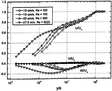
Figure 4. U/Uτ, V/Uτ, and W/Uτ mean velocity profiles for the low Reθ water tunnel flows and the Reθ=5940 flow in local free-stream co-ordinates.
Figure 4 shows a comparison of wind tunnel data (Reθ=9520) at Station 5 with the low Reynolds number (Reθ=500, 760, and 890) water tunnel data of Fleming and Simpson (1997) at the same station for flow around the same shaped wing. Both flowfields are subjected to almost the same non-dimensional pressure distributions around the wing. The U/Ue and W/Ue profiles in local free-stream direction coordinates (XFS tangent to Ue) scale fairly well in terms of y/δ in the outer layer, apparently due to the turbulence-dominated transport and skewing of the vorticity in the outer layer, but do not scale well in wall variables. The largest Reynolds number effect among these cases is the increase in mean crossflow velocity with Reynolds number. The relative increase in viscous forces in the near-wall region at low Reynolds numbers tends to keep the boundary layer mean flow more closely aligned with the free-stream direction.
In wind tunnel or approach flow co-ordinates, Figures 5 and 6 show recent 3-velocity-component LDV mean-velocity-profile data for an approach Reθ=23000 (Ue=30.8 mps) case (Ölçmen and Simpson, 1999). The 2-D zero-pressure-gradient flow mean and turbulence data (Reθ=23000) taken without the presence of the wing agreed with the DNW hot-wire anemometer data where it was available (Dussage et al., 1996; Fernholz et al. 1995; Nockemann et al. 1994). In fact, because of
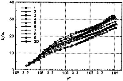
Figure 5. U/Uτ vs. y+ mean velocity profiles of the Reθ=23000 flow in wind tunnel co-ordinates.
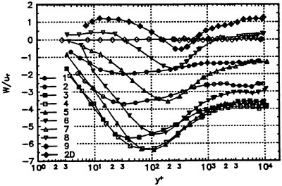
Figure 6. W/Uτ vs. y+ mean velocity profiles of the Reθ=23000 flow in wind tunnel co-ordinates.
the finer spatial resolution of the current LDV system, the current data capture reasonably higher u’ values near the wall where the DNW hot-wire sensors did not have sufficient spatial resolution. The skin-friction values used in Uτ were obtained by fitting the viscous sublayer mean velocity profiles. As in other 3-D data sets, there is no universal law-of-the-wall profile. The crossflow or W data for this case show a very interesting feature in Figure 6. There is no ∂W/∂y or mean streamwise
vorticity in the outer layer until about Station 7. This is in contrast to the water tunnel data and lower Reθ wind tunnel case where ∂W/∂y is non-zero in the outer layer even at Station 1.
This can be explained by the fact that mean streamwise vorticity originates at the wall by a spanwise pressure gradient. For the two flow cases, the non-dimensional pressure gradients produced by the presence of the wing are roughly the same and the wall shear velocity, Uτ, is about 10% higher for the higher Reθ. Thus, the non-dimensional streamwise vorticity flux is about the same for the 2 cases. However, the shear layer thickness produced by the upstream flow is about 150 mm as compared to 39 mm for the Reθ=5940 case. Thus, the streamwise vorticity does not diffuse completely through the thicker outer layer until much farther downstream.
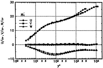
Figure 7. U/Uτ, V/Uτ, and W/Uτ vs. y+ mean velocity profiles at Station 5 of the Reθ=5940 and 23000 flow in wind tunnel co-ordinates.
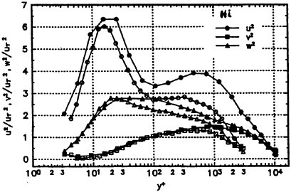
Figure 8. u’2/Uτ2, v’2/Uτ2, and w’2/Uτ2 vs. y+ normal stress profiles at Station 5 of the approach Reθ=5940 and 23000 flows in wind tunnel co-ordinates.
Figures 7–9 show the Station 5 results for these 2 cases. The U/Uτ, W/Uτ, v’/Uτ, and shear stresses profiles show very little Reθ dependence in wall variables for y+<400, while u’/Uτ and w’/Uτ are strongly affected. Fleming and Simpson (1997) also found that v’/Uτ for y+<60 had a weak Reθ dependence in wall variables, while u’/Uτ and w’/Uτ are strongly dependent. This indicates that the active motions which produce the controlling shearing stresses are closely related to v’.
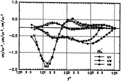
Figure 9. uv/Uτ2, vw/Uτ2, and uw/Uτ2 vs. y+ shear stress profiles at Station 5 of the Reθ=5940 and 23000 flow in wind tunnel co-ordinates.
Like the magnitude of the shearing stress ![]()
![]() that is parallel to the flat wall, the turbulence kinetic energy q2/2=(u’2+v’2+w’2)/2 and the ratio of the two parameters (|τ/ρ|/(q2/2)=2a1) are independent of rotation about the y axis. As shown by Ö1çmen and Simpson (1995a) for the lower Reθ wind tunnel data, Figure 10 shows that a1 does not collapse the higher Reθ data for all stations. Figure 11 shows that Station 5 data for a1 over all available Reθ do not agree.
that is parallel to the flat wall, the turbulence kinetic energy q2/2=(u’2+v’2+w’2)/2 and the ratio of the two parameters (|τ/ρ|/(q2/2)=2a1) are independent of rotation about the y axis. As shown by Ö1çmen and Simpson (1995a) for the lower Reθ wind tunnel data, Figure 10 shows that a1 does not collapse the higher Reθ data for all stations. Figure 11 shows that Station 5 data for a1 over all available Reθ do not agree.
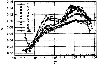
Figure 10. A1 vs. y+ profiles for the Reθ=23000 flow.
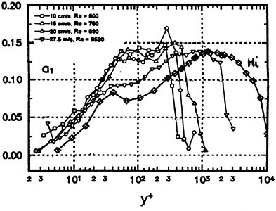
Figure 11. A1 vs. y+ profiles at Station 5 of the water tunnel and approach Reθ=5940 and 23000 wind tunnel flows.
On the other hand, the parameter |τ/ρ|/v’2=1/S and its reciprocal are also independent of rotation about the y axis and seem to be independent of Reθ and 3-D flow condition. For 2-D flows, S is near unity in the semi-log mean velocity profile region. For this 3-D flow, S is nearly a constant over an order of magnitude of y for a given profile. Ölçmen and Simpson (1995a) examined 9 other pressure-driven and shear-driven data sets and concluded that S is also about constant for a given profile for y+>50 and y/δ<0.6, with values between 1 and 2. At stations where the 3-D effects are largest, S is higher than obtained for 2-D flows, which is due to less correlation between the u and v velocity fluctuation components. As shown by Ölçmen and Simpson (1995a) for the lower Reθ wind tunnel data, Figure 12 shows that 1/S correlates the data at all stations. Figure 13 shows almost no effect of Reynolds number on S in the near wall region at Station 5. At y+ down to 30 the data agree. (The departure of the nearest wall data from a common correlation is believed to be due to high measured values of v’ as the wall is approached.) Fleming and Simpson (1997) show that the profiles of ![]() and
and ![]() at Station 5, over the large Reynolds number range 500<Reθ<9520 do not correlate in inner variables or outer variables, while 1/S collapses in inner variables. This is in contrast to a1, which varies much with 3-D effects and Reynolds number.
at Station 5, over the large Reynolds number range 500<Reθ<9520 do not correlate in inner variables or outer variables, while 1/S collapses in inner variables. This is in contrast to a1, which varies much with 3-D effects and Reynolds number.
On physical grounds, v’ should be an important turbulence velocity scale, especially near the wall since the shear-stress-producing ejections and sweeps strongly determine v’. The a1 parameter contains the highly Reθ dependent u’2 in the TKE, which reflects some of the inactive low frequency motions that do not contribute to the shear-stress producing motions. The parameter S directly relates this scale v’ to the desired shearing stress
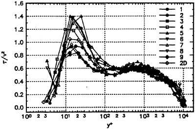
Figure 12. 1/S vs. y+ profiles for the Reθ=23000 flow.
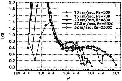
Figure 13. 1/S vs. y+ profiles at Station 5 of the water tunnel and approach Reθ=5940 and 23000 wind tunnel flows.
|τ/ρ| to help provide closure on a turbulence model.
Another phenomenon occurs for the flowfield shown in Figure 1. For a sufficiently blunt nose, such as this wing, the horseshoe vortex structure between the vortex and the flat wall shows aperiodic low-frequency chaotic switching between velocity states that produce double-peaked (bimodal) velocity histograms of the velocity component spanwise to the vortical core direction. This self-induced large-scale unsteadiness of wing/body junction nose separations is responsible for high surface pressure fluctuations and high heat transfer rates around the nose. These chaotic vortices are produced by the 3-D separation in front of the nose; multiple unsteady vortices are present in this region that can merge and are stretched around the wing. These chaotic intermittent vortical structures also produce very large apparent Reynolds-averaged stress values because their unsteady flow effects are averaged with smaller-scaled turbulent contributions. In one mode the
flow is nearly tangent to the wing while in the other mode higher velocity flow is swirled down near the wing from near the free stream by the vortical motion. Near the flat wall, the latter mode flow is at a large angle to the wing surface. Simpson (1996) in his review and Ölçmen and Simpson (1997b) give many more details and examples of the features of this flow behavior, which appears to be present in all turbulent wing/body junction cases with sufficient nose bluntness.
Clearly, it is inappropriate to combine the effects of these large-scale separation-induced chaotic vortices with the turbulence structure, but some continue to ignore this physical feature in calculations (Rizzi and Vos, 1998). A seemingly proper way to model the horseshoe vortex flow around the wing is to use a large-eddy simulation for the chaotic scales, which are more coherent, and a subgrid model for the less coherent turbulence that accompanies the boundary layer that approaches the wing.
Some Modeling Equations
It appears clear that the isotropic eddy viscosity approach to 3DTBL modeling does not capture the flow physics. As a result of the limitations of algebraic models to mimic the observed lags within these flows, a 3-Reynolds-stress transport equation model is suggested with the normal-to-wall rms velocity fluctuation v’ as the velocity scale, since v’2 correlates well with the shearing stress magnitude |τ/ρ|. Clearly, this model cannot mimic the nature of the low-frequency chaotic horseshoe vortices mentioned above.
Observations presented in this paper suggest that transport equations are required to account for: (1) the variable anisotropy of the eddy viscosities, (2) the lags between the mean flow and the turbulence field, and (3) the strong relation between the important shearing stresses and v’:
x-direction momentum equation:
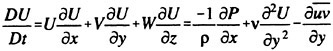
(1)
z-direction momentum equation:
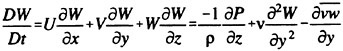
(2)
Continuity equation:
(3)
In addition to the momentum and continuity equations, transport equations for uv, -vw, and v2 are required:
(a) transport of -uv stress:
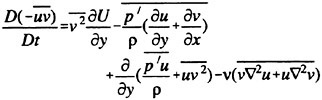
(4)
(b) transport of -vw stress:
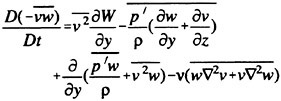
(5)
(c) transport of -v2 stress:
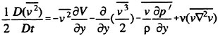
(6)
Algebraic relations among some of the parameters in these equations have been revealed from the data base of 3-D experiments examined by Ciochetto and Simpson (1995, 1997). Eleven data sets encompassing several different test geometries were examined: Pompeo et al. (1992, 1993) plane of symmetry flows with spanwise rates-of-strain; Schwarz and Bradshaw (1992, 1993) 30° bend flow; Ölçmen and Simpson (1995a) wing/body junction flow; Baskaran et al. (1990) pressure-driven flows with wall curvature; Chesnakas and Simpson (1992, 1994, 1997), Kreplin and Stäger (1993), and Barberis and Molton (1993) leeside flows on axisymmetric bodies at angles of attack; Devenport and Simpson (1990) and McMahon et al. (1982) wing/body vortex flows; and Driver and Johnston (1990) and Littell and Eaton (1991) shear-driven flows.
In these data sets, the S=v’2/|τ/ρ| parameter correlates fairly well from station to station within a flow and between experiments, as long as embedded mean flow vortices are not present. The ratio 1/S approximates a constant for 0.3–0.4<y/δ<0.7–0.8 ranging from values of 0.5–0.8 with an overall average of approximately 0.7. At y/δ=1.0, 1/S appears to have a mean value, for the data presented, of approximately 0.3. The parameter appears to be mildly affected by different 3D effects, however the effects were of the order of the uncertainty in the experiments. Such effects include a noticeable decrease in the crossflow decay region of the Schwarz and Bradshaw experiment, a slight rise at the aft end of the prolate spheroid flows of Kreplin and Stäger and Chesnakas and Simpson due to separation vortices, and a lower value in the decay region of Driver. It did, however, maintain consistent values for the Baskaran et al. flows and the experiments of Littell and Eaton. All of the other parameters investigated for the
experiment of Littell and Eaton had completely different behavior from the other 3D experiments, only 1/S exhibited behavior consistent with all of the other 3D TBLs. The experiments in the horseshoe vortex region of the wing-body junction failed to produce good behavior of the 1/S parameter. This is surmised to result from the significant wall-normal component of velocity and the chaotic vortical structure.
Some algebraic parameters describing the turbulent triple products are also rather insensitive to three-dimensional effects. They also maintain a constant value for the outer part of the 3D TBL. The ![]()
![]() parameter is invariant to rotation about the y axis and relates the turbulent transport of the instantaneous stresses
parameter is invariant to rotation about the y axis and relates the turbulent transport of the instantaneous stresses ![]() and
and ![]() in the y direction, as given in eqn. (4–6). This parameter tends to approximate a constant value of 0.85±0.15 for 0.3≤ y/δ≤0.7–1.0. The values for each station are a very good approximation to a constant in this region for the experiments examined by Ciochetto and Simpson. This strongly indicates that the same outer region intermittent coherent structure flow phenomena produce these triple products, even for the convex curved wall and line of symmetry flows. Figure 14 also shows the same behavior for B2 for the Reθ=23200 flow.
in the y direction, as given in eqn. (4–6). This parameter tends to approximate a constant value of 0.85±0.15 for 0.3≤ y/δ≤0.7–1.0. The values for each station are a very good approximation to a constant in this region for the experiments examined by Ciochetto and Simpson. This strongly indicates that the same outer region intermittent coherent structure flow phenomena produce these triple products, even for the convex curved wall and line of symmetry flows. Figure 14 also shows the same behavior for B2 for the Reθ=23200 flow.
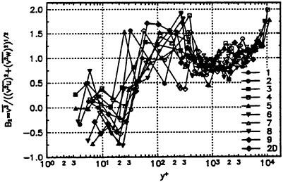
Figure 14. B2 vs. y+ for the Reθ=23200 flow.
The parameter ![]() which is also invariant to y-axis rotation, maintains better correlation across the TBL and from experiment to experiment than the B2 parameter. It seems to hold even for the leeside vortex flow of Kreplin and Stäger. It maintains a value of 0.3–0.4 for y/δ>0.4 and tends to extend farther towards the wall for the upstream stations in a given experiment. These results indicate that the turbulent transport of TKE is closely related to the v transport of v2 and could simplify outer region modeling. Surface convex curvature does not have much effect on this conclusion. Figure 15 also shows the same behavior for B for the Reθ=23200 flow.
which is also invariant to y-axis rotation, maintains better correlation across the TBL and from experiment to experiment than the B2 parameter. It seems to hold even for the leeside vortex flow of Kreplin and Stäger. It maintains a value of 0.3–0.4 for y/δ>0.4 and tends to extend farther towards the wall for the upstream stations in a given experiment. These results indicate that the turbulent transport of TKE is closely related to the v transport of v2 and could simplify outer region modeling. Surface convex curvature does not have much effect on this conclusion. Figure 15 also shows the same behavior for B for the Reθ=23200 flow.
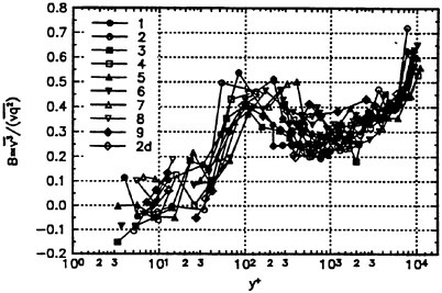
Figure 15. B vs. y+ for the Reθ=23200 flow.
Examination of Other Model Equations
The data sets used above provide some insights into some algebraic relations, mainly in the outer and logarithmic velocity profile regions, between v’2 and |τ/ρ| and among several triple-product turbulent diffusion terms which are strongly correlated in a variety of pressure-driven 3D non-equilibrium turbulent flows. However, additional relationships are needed to complete the closure of a calculation method. The viscous dissipation term in equation (6) needs to be modeled, while the viscous terms in each of equations (4) and (5) are almost negligible except near the wall. The pressure diffusion and pressure/rate-of-strain terms in equations (4–6) need to be modeled.
Ölçmen and Simpson (1996b,c,d; 1997a) examined several second-order closure models in light of their detailed experimental data (Ölçmen and Simpson, 1997b) obtained for a 2DTBL and several locations shown in Figure 1 for the wing/body junction wind tunnel flow. Enough spatial data were obtained to determine the convective terms from data and perform a term-by-term examination of the Reynolds-stress transport equation budgets (Ölçmen and Simpson, 1996b). All terms except the dissipation (ε), pressure diffusion, and pressure/rate-of-strain (PRS) terms were evaluated directly using data.
Using the TKE transport equation and Lumley’s (1978) pressure diffusion model, the dissipation rate ε was obtained from the difference among other terms. The Hallbäck et al. (1990) anisotropic dissipation distribution was used and produced stress transport equation budgets that were in better agreement with low Reynolds number direct numerical simulation (DNS) budgets than the isotropic dissipation case.
The resulting pressure/rate-of-strain (PRS) terms for each transport equation and flow location were then compared by Ölçmen and Simpson (1996b,c,d)
with 7 models. The Fu et al. (1987) pressure/rate-of-strain model (labeled FLT1) as it was modified by Shih and Lumley (1993) (labeled FLT2) worked best among the tested models for the 2D flow normal stresses. The Shih-Lumley/Choi-Lumley (SLCL) (1984) PRS model worked best for the ![]() shearing stress transport equation for the 2D flow.
shearing stress transport equation for the 2D flow.
The FLT2 PRS model for the v’2 transport equation worked best for the 3D flow stations that were tested which were away from the chaotic bimodal vortices that were mentioned above. For the same stations, the PRS terms in the shear stress transport equations were best described by the FLT1 and SLCL models. There is still a need for improved PRS models for 3D flows, especially near the wall in the -vw shearing stress transport equation.
Ölçmen and Simpson (1997a) used several turbulent diffusion models to compare with the experimentally measured profiles. All models that were tested failed to capture the magnitude of the triple products, apparently due to the scaling factor q2/ε. Note that since the experimentally measured turbulent diffusion terms were used in the transport equation budgets, Ölçmen and Simpson’s conclusions about the PRS models do not depend upon a turbulent diffusion model.
Concluding Comments and Future Work
Because of the non-equilibrium nature of 3D turbulent boundary layers, it is necessary to use Reynolds-averaged transport equations which can mimic the lags between the mean flow and the shearing stress structure. Work discussed and referenced here show that v’ is closely related to the shear stress magnitude by S in a variety of non-equilibrium 3D experiments over a range of Reynolds numbers. The parameters ![]()
![]() are nearly constant across the outer boundary layer in these flows.
are nearly constant across the outer boundary layer in these flows.
These parameters alone are not enough for closure and relationships for the pressure diffusion, pressure/rate-of-strain (PRS), turbulent diffusion, and dissipation are needed. The work quoted here shows that several uncertainties exist in the modeling of these terms, especially in the near-wall region. Better models for the turbulent diffusion are needed. The relationships among pressure and velocity fluctuations remains an important modeling issue. Data are needed for the pressure diffusion and PRS in order to verify existing models and to develop better models.
Since the direct measurement of the pressure fluctuation within these flows is presently unfeasible with a fine-resolution sensor, one must use the Poisson volumetric integral of the turbulent velocity fluctuation correlation contributions to the pressure fluctuation (Chou, 1945). To this end, recently considerable vi-vj and vi-vj2 LDV spatial correlation wind tunnel data have been obtained for a 2-D TBL and at Station 5 of the wing/body junction wind tunnel flow (Ölçmen et al. 1998). These data are being used in the Poisson pressure-fluctuation volume integral in order to better understand the effects of 3-D skewing on the pressure-fluctuation structure.
Acknowledgment
Portions of the referenced work at VPI&SU have been supported by: Office of Naval Research (current Grant N00014–94–1–0092; Dr. L.P.Purtell, Program Manager). The authors gratefully acknowledge this support.
References
1. Ailinger, K.G. and Simpson, R.L. (1990) Measurements of Surface Shear Stresses under a Three-Dimensional Turbulent Boundary Layer Using Oil-Film Laser Interferometry, VPI-AOE-173; DTIC Report ADA2294940XSP.
2. Barberis, D. and Molton, P. (1993) Experimental Study of 3-D Separation on a Large Scale Model, AIAA 24th Fluid Dynamics Conference, Orlando, FL USA, AIAA-93–3007.
3. Baskaran, V., Pontikis, Y.G., and Bradshaw, P. (1990) An Experimental Investigation of a Three-dimensional Turbulent Boundary Layer on ‘Infinite’ Swept Curved Wings,” J. Fluid Mech., Vol. 211, p. 95–122.
4. Chesnakas, C.J., Simpson, R.L., and Madden, M.M. (1994) Three-dimensional Velocity Measurements on a 6:1 Prolate Spheroid at 10° Angle of Attack, VPI-AOE-202REV; DTIC report ADA2764850XSP.
5. Chesnakas, C.J. and Simpson, R.L. (1992) An Investigation of the Three-dimensional Turbulent Flow in the Cross-flow Separation Region of a 6:1 Prolate Spheroid, Sixth International Symposium on Applications of Laser Techniques to Fluid Mechanics, Lisbon, Portugal, 20–23 July, 1992; Exp. in Fluids, Vol. 17, pp. 68–74, 1994.
6. Chesnakas, C.J. and Simpson, R.L. (1997) Detailed Investigation of the Three-Dimensional Separation About a 6:1 Prolate Spheroid, AIAA Journal,
Vol. 35, no. 6, pp. 990–999.
7. Choi, K.S. and Lumley, J.L. (1984) Turbulence and Chaotic Phenomena in Fluids, Proceedings IUTAM Symposium (Kyoto, Japan), edited by T.Tatsumi, North-Holland, Amsterdam, p. 267.
8. Chou, P.Y. (1945) On Velocity Correlations and the Solutions to the Equations of Turbulent Motions, Quarterly Applied Math., vol. 3, pp. 38–54.
9. Ciochetto, D.S. and Simpson, R.L. (1995) An Investigation of 3-D Turbulent Shear Flow Experiments and New Modeling Parameters, Turbulent Shear Flows 10, pp. 7–25 thru 7–30, Penn State, August 14–16, 1995.
10. Ciochetto, D.S. and Simpson, R.L. (1997) Analysis of Three-Dimensional Turbulent Shear Flow Experiments with Respect to Algebraic Modeling Parameters, Report VPI-AOE-248, submitted to DTIC.
11. Devenport, W.J. and Simpson, R.L. (1990) A Time-dependent and Time-averaged Turbulence Structure Near the Nose of a Wing-body Junction”, J. Fluid Mech., 210, pp. 23–55.
12. Devenport, W.J. and Simpson, R.L. (1990) The Flow Past a Wing-body Junction—an Experimental Evaluation of Turbulence Models, 18th Symposium on Naval Hydrodynamics, August 20–22, Ann Arbor, Michigan; also AIAA J., 30, pp. 873–881, 1992.
13. Devenport, W.J. and Simpson, R.L. (1990) An Experimental Investigation of the Flow Past an Idealized Wing-body Junction,” VPI&SU Report VPI-AOE-172; DTIC report ADA2296028XSP.
14. Driver, D.M. and Johnston, J.P. (1990) Experimental Study of a Three-dimensional Shear-driven Turbulent Boundary Layer with Streamwise Adverse Pressure Gradient,” NASA TM 102211; also Report MD-57, Thermo. Div., Dept. Mechanical Engineering, Stanford University.
15. Dussauge, J., Fernholz, H., Finley, P., Smith, R., Smits, A., and Spina, E. (1996) Turbulent Boundary Layers in Subsonic and Supersonic Flow, AGARD-AG-335.
16. Fernholz, H.H., Krause, E., Nockemann, M., and Schober, M. (1995) Comparative measurements in the canonical boundary layer at Reθ≤6×10⁴ on the wall of the German-Dutch windtunnel, Phys. Fluids, Vol. 7, no. 6, pp.1275–1281.
17. Fleming, J.L. and Simpson, R.L. (1997) Experimental Investigation of the Near Wall Flow Structure of a Low Reynolds Number 3-D Turbulent Boundary Layer,” Report VPI-AOE-247, submitted to DTIC.
18. Fleming, J., Simpson, R.L., and Devenport, W.J. (1991) An Experimental Study of a Turbulent Wing-body Junction and Wake Flow, VPI-AOE-179; DTIC Report ADA2433886XSP; AIAA-92–0434; Exp. Fluids, 14, pp. 366–378, 1993.
19. Fu, S., Launder, B.E., and Tselepidakis, D.P. (1987) Accommodating the Effects of High Strain Rates in Modeling the Pressure-strain Correlation, UMIST Mechanical Engineering Dept. Rept. TFD/87/5.
20. Ha, S. and Simpson, R.L. (1993) An Experimental Investigation of a Three-dimensional Turbulent Boundary Layer Using Multiple-sensor Probes, Ninth Symposium on Turbulent Shear Flows, Kyoto, Japan, 16–18 Aug. 1993, p. 2–3–(1–6).
21. Hallbäck, M., Groth, J., and Johansson, A.V. (1990) An Algebraic Model for Nonisotropic Turbulent Dissipation Rate in Reynolds Stress Closure, Phys. Fluids A, vol. 2, no. 10, pp. 1859–1866.
22. Johnston, J.P. and Flack, K.A. (1996) Review—Advances in Three-Dimensional Turbulent Boundary Layers with Emphasis on the Wall-Layer Regions, J. Fluids Engineering, Vol. 118, no. 2, pp. 219–232.
23. Kreplin, H.P. and Stäger, R. (1993) Measurements of the Reynolds Stress Tensor in the Three Dimensional Boundary Layer of an Inclined Body of Revolution, Ninth Symposium on Turbulent Shear Flows, Kyoto, Japan, 16–18 Aug. 1993, p. 2–4–(1–6).
24. Lewis, D.J., Simpson, R.L., and Diller, T. (1993) Time-Resolved Surface Heat Flux Measurements in the Wing/body Junction Vortex, AIAA-93–0291, AIAA 31st Aerospace Sciences Meeting, Reno, NV, Jan. 11–14; also AIAA J. Thermo. and Heat Trans., 8, pp. 656–663, 1994.
25. Lewis, D.J. and Simpson, R.L. (1996) An Experimental Investigation of Heat Transfer in Three-dimensional and Separating Turbulent Boundary Layers, VPI-AOE-229; submitted to DTIC.
26. Lewis, D.J. and Simpson, R.L. (1998) Turbulence Structure of Heat Transfer Through a Pressure-driven Three-dimensional Turbulent Boundary
Layer, AIAA J. of Thermophysics and Heat Transfer, Vol. 12, 2, pp. 248–255, April–June.
27. Littell, H.S. and Eaton, J.K. (1991) An Experimental Investigation on the Three-dimensional Boundary Layer on a Rotating Disk, Thermo. Div., Dept. Mechanical Engineering, Stanford Univ., Report No. MD-60.
28. Lumley, J.L. (1978) Computation and Modeling of Turbulent Flows, Adv. in Applied Mech., vol. 18, pp. 124–176.
29. McMahon, H., Hubbartt, J., and Kubendran, L. (1982) Mean Velocities and Reynolds Stresses in a Juncture Flow, NASA CR-3605.
30. Nockemann, M., Abstiens, R., Schober, M., Bruns, J., and Eckert, D. (1994) Messungen in einer turbulenten Wandgrenzschicht bei grossen Reynolds-Zahlen im Deutsch-Niederländischen Windkanal Messbereicht, Aero. Inst., Tech. Hochschule Aachen, Germany.
31. Ölçmen, S.M. and Simpson, R.L. (1990) An Experimental Investigation of Pressure-Driven Three-dimensional Turbulent Boundary Layer. VPI-AOE-178; DTIC Report ADA2294957XSP.
32. Ölçmen, S.M. and Simpson, R.L. (1995a) An Experimental Study of Three-dimensional Pressure-Driven Turbulent Boundary Layer, J. Fluid Mech., 290, pp. 225–262.
33. Ölçmen, S.M. and Simpson, R.L. (1995b) A 5-Velocity-Component Laser-Doppler Velocimeter for Measurements of a Three-Dimensional Turbulent Boundary Layer, paper 4.2, Seventh International Symposium on Applications of Laser Techniques to Fluid Mechanics, 11–14, July, 1994, Lisbon, Portugal; revised version Invited Paper, Measurement Science and Technology, 6, pp. 702–716, 1995. Highlighted in The Year in Review, Fluid Dynamics, pp. 20–21, Aerospace America, Vol. 33, no. 12, Dec. 1995.
34. Ölçmen, S.M., and Simpson, R.L. (1996a) An Experimental Study of a Three-Dimensional Pressure-Driven Turbulent Boundary Layer: Data Bank Contribution, J. Fluids Engineering, vol. 118, pp. 416–418, 1996.
35. Ölçmen, S.M., and Simpson, R.L. (1996b) Experimental Transport-rate Budgets in Complex Three-dimensional Turbulent Flows at a Wing/Body Junction, 27th AIAA Fluid Dynamics Conference, AIAA-96–2035, New Orleans, LA, June 17–20.
36. Ölçmen, S.M., and Simpson, R.L. (1996c) Theoretical and Experimental Pressure-strain Comparison in a Pressure-driven Three-dimensional Turbulent Boundary Layer, 1st AIAA Theoretical Fluid Mechanics Meeting, AIAA-96–2141, New Orleans, LA, June 17–20.
37. Ölçmen, S.M. and Simpson, R.L. (1996d) Experimental Evaluation of Pressure-Strain Models in Complex 3-D Turbulent Flow Near a Wing/Body Junction, VPI-AOE-228; DTIC Report ADA3071164XSP.
38. Ölçmen, S.M. and Simpson, R.L. (1996e) Higher Order Turbulence Results for a Three-Dimensional Pressure-Driven Turbulent Boundary Layer, VPI-AOE-237; submitted to DTIC.
39. Ölçmen, S.M. and Simpson, R.L. (1997a) Experimental Evaluation of Turbulent Diffusion Models in Complex 3-D Flow Near a Wing/Body Junction, AIAA-97–650, 35th AIAA Aerospace Sciences Meeting, Jan. 6–10.
40. Ölçmen, S.M. and Simpson, R.L. (1997b) Some Features of a Turbulent Wing-Body Junction Vortical Flow, AIAA-97–0651, 35th AIAA Aerospace Sciences Meeting, Jan. 6–10; VPI-AOE-238 submitted to DTIC, 1996.
41. Ölçmen, S.M. and Simpson, R.L. (1997c) Higher Order Turbulence Results for a Three-Dimensional Pressure-Driven Turbulent Boundary Layer, under revision for J. Fluid Mechanics, 1997.
42. Ölçmen, S.M., Simpson, R.L. and George, J. (1999) Experimental Study of a High Reynolds Number (Reθ=23000) Turbulent Boundary Layer Around a Wing-Body Junction, submitted for 37th AIAA Aerospace Sciences Meeting, Jan..
43. Ölçmen, S.M., Simpson, R.L. and Goody, M. (1998) An Experimental Investigation of Two-Point Correlations in Two- and Three-Dimensional Turbulent Boundary Layers, AIAA-98–0427, 36th AIAA Aerospace Sciences Meeting and Exhibit, Jan. 12–15.
44. Pompeo, L.P. (1992) An Experimental Study of Three-dimensional Turbulent Boundary Layers, Ph.D. Diss., ΕΤΗ no. 9780, Swiss Fed. Inst. Tech., Zurich.
45. Pompeo, L.P., Bettelini, M.S.G., and Thomann, H. (1993) Laterally Strained Turbulent Boundary Layers Near a Plane of Symmetry, J. Fluid Mech., Vol. 257, pp. 507–532.
46. Rizzi, A. and Vos, J. (1998) Towards Establishing Credibility in Computational Fluid Dynamics Simulations, AIAA Journal, Vol. 36, no. 5, pp. 668–675.
47. Schwarz, W.R. and Bradshaw, P. (1992) Three-dimensional Turbulent Boundary Layer in a 30 Degree Bend: Experiment and Modeling, Thermosciences Division Report No. MD-61, Stanford.
48. Schwarz, W.R. and Bradshaw, P. (1993) Measurements in a Pressure Driven Three-dimensional Turbulent Boundary Layer During Development and Decay, AIAA Journal, Vol. 31, No. 7, p. 1207–1214.
49. Shih, T.H. and Lumley, J.L. (1993) Critical Comparison of Second-order Closures with Direct Numerical Simulations of Homogeneous Turbulence, AIAA Journal, Vol. 31, no. 4, pp. 663–670.
50. Simpson, R.L. (1996) Aspects of Turbulent Boundary Layer Separation, Prog. Aerospace Sci., Vol. 32, pp. 457–521.
Investigation of Viscous Flow Field Around an Appended Revolution Body with Guide Vane Propeller
L.-D.Zhou (China Ship Scientific Research Center, China),
F.Zhao (National Laboratory of Hydrodynamics, China)
Abstract
A RANS solver is presented to numerically simulate the viscous wake of an appended revolution body with guide vane propeller at Reynolds number 107. The k-ε turbulence model together with wall function is used. The resulting finite difference equations are solved by SIMPLEC, ADI. The technique of rising up the bottom surface is presented to overcome radial contraction problem in Cartesian coordinate system. The three dimensional body forces are separately adopted to model the affection of the guide vane and propeller. The detailed flow characteristics, especially the counter-swirl component generated by the guide vane in the propeller inflow are numerical seized successfully. Comparing with the experimental data, computational axial velocity on the propeller disk plane comes up to engineering requirement.
1. Introduction
The flow around an appended revolution body at high Reynolds number is part of a competitive benchmark problem to evaluate existing computational fluid dynamics (CFD) capabilities for incompressible viscous flow.
There are always appendages equipped in the submarine’s stern. The interaction of flow around the hull/appendage creates complex juncture vortices shedding downstream. Thus, the flow into the propulsor becomes quite complex and non-uniform even in steady straight motion. Such undesired inflow may cause propulsor efficiency decreased and generate noise. The prediction of this flow is of great importance to the propeller designer.
To numerical simulate this complicated inflow to the propulsor for an appended submarine configuration, the current rapidly developed computational fluid dynamics has provided an effective and feasible approach. The powerful combination of interactive computer-aided design (CAD) and grid generation packages allow one to model and generate grids quite effectively around such complicated geometry. In addition, the numerical techniques to solve the Navier-Stokes equation has been substantially improved in the areas of accuracy, robustness and computational speed. Also, the multi-zonal concept has proven to be quite capable in effectively handling complicated grid topology resulting from complex hull/appendages configurations. For a zone with appendages, using the multiblock grid structure, we could solve the 3-D Reynolds-averaged Navier-Stokes equations in a simple region (without any appendage). The treatment of the interface boundary between neighboring zones and sub-blocks is very important. Authors have developed a multiblock grid generation [1] and corresponding flow field multiblock coupled computational method [2].
It is well known that the adoption of stators locating in front of propeller can result in a reduction of rotational energy losses, so that propulsion efficiency could be increase. In addition, a non-axisymmetric upstream stator can alter the inflow to downstream propeller in such a way that unsteady forces and cavitation could be reduced. The Guide Vane, as an effective equipment of improving the inflow of the propeller, has been adopted in surface ship design.
Recently, Professor Shen H.C. et al were taking the lead in Guide Vane design for submergible appended revolution body [4]. The Guide Vane is composed of 4 radially placed vanes of aerofoil section and installed at an appropriate position between the stern appendages and propeller. By adopting guide vane, the inflow state of propeller and the interactions among ship hull, appendages and propeller were regulated, so that powering performance could be improved and noise reduced.
Based on the model experimental results [4], about 5~10 percent saving of DHP and 2~3 dB noise reduction were expected. Regarded as a special appendage of submergible body, the Guide Vane is simple to construct, easy to manufacture and convenient to install. It should be thought as a promising practical device for submergible vehicles. Besides experimental research, CFD is very helpful to understand the flow structure around vane and in the wake, and also to evaluate and optimize the design of guide vane. The purpose of this paper is trying to develop an effective and practicable CFD method in the guide vane design.The
purpose of this paper is trying to develop an effective and practicable CFD method in the guide vane design. The geometry of a general submergible body is composed of streamlined appendages (one sail and four fins) attached to an axisymmetric hull. The whole flow field around this appended revolution body is divided into two big zones, sail zone and fins zone. The detailed results of the sail zone was proposed in authors’ earlier papers [2]~[3]. In this paper, the fins zone with and without guide vane is specially presented. A 3-D RANS equation solver [3] is applied to predict the viscous wake of an appended submergible body. The k-ε two equations turbulence model together with wall function are used. The resulting finite difference equations discreted in non-staggered grid system are solved by SIMPLEC, ADI. Computational Reynolds number is 107.
The guide vane is also a kind of thin foil body located between fins and propeller, something like a steady propeller, as shown in Fig. 1. So, the body force model is used in the present paper to simulate the action of propeller and also the guide vane. Using the panel method [5], the distribution of 3-D body force by the guide vane and propeller are both gotten. These additional source items, substituted into RANS equations at proper grid nodes, are the representation of the guide vane and propeller respectively.
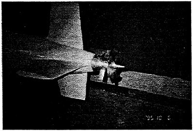
Fig. 1 Illustration of guide vane location
A couple of plotting package is also integrated into the system for the efficient visualization of computed results and for the meaningful comparison with experimental data or other numerical results. The numerical results have been compared with experimental data in wake and on the propeller disk plane. It shows that most of the important features of the mean flow, such as block effect of appendages, preswirl of guide vane and drawing of propeller, could be successfully predicted. Instead of many qualitative contours or vectors, the most important and interesting quantitative data of the nominal mean velocity radial distributions on the propeller disk plane were provided here. The average error of comparison data between the computation and the experimental data in wind tunnel is 2.54% for guide vane case, and 4.63% without guide vane.
2. Numerical Method
2.1 Governing Equations
We consider the governing equations in Cartesian coordinate (xi,t)=(x,y,z,t) for unsteady, three-dimensional, incompressible flow. The complete three-dimensional Reynolds-averaged equations in the general form are
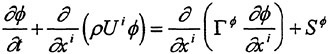
(1)
which ![]() represents any one of the convective transport quantities (1,U,V,W,k,ε). The scalar diffusivity
represents any one of the convective transport quantities (1,U,V,W,k,ε). The scalar diffusivity ![]() and source terms
and source terms ![]() for Ui, k and ε respectively are
for Ui, k and ε respectively are
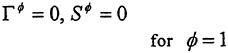
(2a)
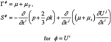
(2b)
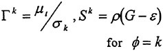
(2c)
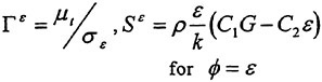
(2d)
2.2 Body-fitted Grid System
For the present application to the flow around an appended submergible body, a single integrated numbering grid system is very difficult to generate. The idea of multizone and multiblock is
adopted in grid generation and flow solver. The whole appended submergible body external flow field was divided into two big zones, the one is the front part of the submergible body, hull with sail, the other is stern part, body with fins. For the sail zone, a multiblock grid generation method [1] is used to generate body-fitted grid surrounding the sail. The computation of flow field also used multiblock coupled method [2].
The body-fitted numerical grids were generated by a system of elliptic partial differential (Poisson) equations of the form of
(3)
here, ∇2 is the Laplacian operator in Cartesian coordinates xi. The nonhomogeneous source function fi may be assigned appropriate values to yield desirable grids distributions. In practical applications, the inverse transformation of equation (3) is used to obtain the coordinate transformation relations xi=xi(ξi), i.e.,
(4)
which ∇2 is the Laplacian operator in the transformed plane (ξi). Using the transformation relations, the equation (4) can be rewritten as
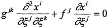
(5)
which gjk is the inverse metric tensor. The grid control function fj were determined by the specified boundary node distribution. In present study, a corrective method is used to generate nearly orthogonal grids [3].
2.3 Rising up of bottom surface
Generally, the hull of submarine is an axisymmetric body, contracting into a point at stern. This will cause grids near the hull converging into one point in Cartesian coordinate system (i.e. r=0 case). To deal with this kind problem, cylindrical coordinate system or some geometry appropriate in the stern may be adopted. The problems with r=0 are solved undoubtedly in cylindrical coordinate system, but many computer codes developed under Cartesian coordinate system could not use directly. Though the stern shape changed a little, the method [6] of trailing out a “thin hub” is often applied to make geometry appropriate. The technique of rising up the bottom surface [7] is presented here to overcome this radial contraction problem in Cartesian coordinate system. Possessing 3-d body-fitted grid generation method, the present paper use TDMBGG software [1], the key of question is how to properly give six surfaces’ grid systems of the controlling volume. Fig. 2 illustrates the six surfaces and computational zone (fins zone). The bottom surface is the hull surface, including wake. During the stern contraction, we should arrange the bottom surface crawl up to both side surfaces. Thus, the good quality grid system could always be gotten, even in r=0 case. Illustrated in Fig. 3 is the process of rising up.
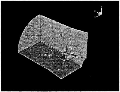
Fig. 2 Six surfaces of fins zone
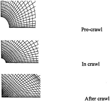
Fig. 3 Process of rising up the bottom surface
2.4 Body force modeling of guide vane and propeller
Using the method in [5], the radial distributions of 3-D body force of guide vane and propeller are given in their located position respectively
(6)
In circumferential direction we share out equally onto their computational grids controlling point
(7)
If the volume of grid unit (i, j, k) is Vol(i, j, k), then the momentum equation could be written as

(8)
where the additional source term ![]() is the affection of guide vane and propeller on their own located computational grids
is the affection of guide vane and propeller on their own located computational grids
(9)
2.5 Numerical algorithm and solution procedure
The discretisation of the governing differential equation and wall function are detailed in reference [7]. Non-staggered grid method is adopted, and velocity-pressure coupling SIMPLEC approach is used. In a time step, the momentum equations are solved first, then, the equations for pressure correction, and the k-ε turbulence model equations are solved last. The iteration is used at two levels, an inner iteration to solve for the spatial coupling of each variable and an outer iteration to solve for coupling between variables. Thus each variable is taken in sequence, regarding all other variables as fixed and reforming coefficients by updated values of the variables. The detailed description was given in reference [2]~[3], [6]~[7].
3. Results and Discussion
In the presented paper, viscous wake of a submarine model with and without guide vane and propeller are numerical simulated. As mentioned above, the computational Reynolds number is 107. All the computation are carried on CONVEX computer with good convergence characteristics. The computational grids are shown in Fig. 4.
There were four computational cases, without guide vane and propeller, with guide vane only, with propeller only and both with guide vane and propeller. The axial drawing of the propeller is shown in Fig. 5. The comparisons of computational velocity vectors on the cross plane after propeller disk are emphatically given in Fig. 6. The main flow characteristics, such as the preswirl affection of guide vane and the reduction of the rotative kinetic energy losses of propeller, are clearly simulated.
Instead of many other qualitative contours or vectors, the present paper specially provides an more interesting quantitative comparison data. Fig. 7 shows the comparison curves of the radial distribution of axial velocities on the propeller disk plane between the computation and the experiment data in wind tunnel. The average error is 2.54% for guide vane case, and 4.63% without guide vane.
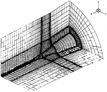
Fig. 4 Computational grids of stern wake
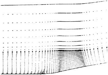
Fig. 5 Axial drawing of the propeller
4. Conclusion
A 3-D RANS solver is applied to predict the viscous wake of an appended submergible body with a guide vane propeller. The technique of rising up the bottom surface is presented to overcome radial contraction problem in Cartesian coordinate system. The 3-D body force model is successfully used to represent the guide vane and propeller actions. The qualitative and quantitative consistence between experiment and calculation is shown. This would prove the present method to be competent at simulation the submergible body wake with guide vane propeller.
Although the validation of this analysis system is not fully completed at the present time, the continuous improvement of system will provide an efficient procedure to evaluate viscous flow phenomena around appended axisymmetric body, with and without guide vane and propeller, such as prediction of nominal wake distribution at the propeller disk plane. Improvements on the accuracy of each module in the system are to be continued necessarily.
5. Acknowledgments
The authors greatly acknowledge to National Laboratory of Hydrodynamics for its Fund supporting.
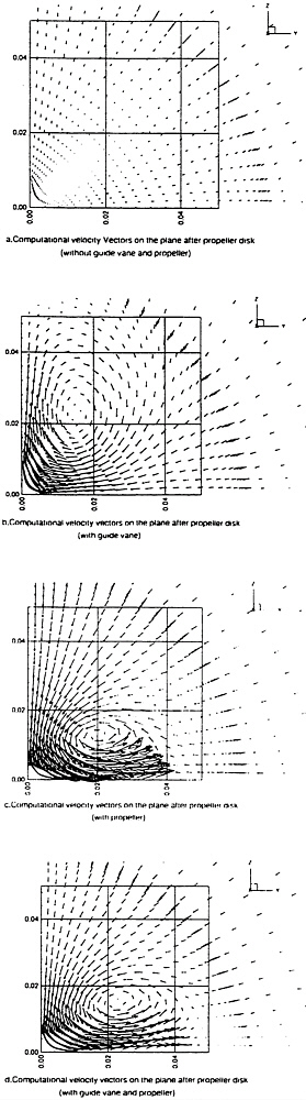
Fig. 6 Computational cross vectors of four cases
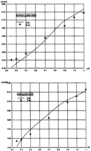
Fig. 7 Comparison curves of axial velocity on the propeller disk plane
6. References
[1] ZHAO, F., ZHOU, L.D., and REN, A.L., “General Coupled Generation Method of 3-D Multiple Block Body-fitted Grid,” Journal of Hydrodynamics, Ser. A, Vol. 9, No. 4, 1994, (in Chinese)
[2] ZHAO, F., and ZHOU, L.D., “Multiblock Coupled Computation of the Viscous Flow Field Around a Submarine Sail Zone,” Journal of Hydrodynamics, Ser. A, Vol. 10, No. 4, 1995, (in Chinese)
[3] ZHAO, F., “Numerical Simulation of the Viscous Flow Around an Appended Submarine Model,” Proc. of Second International Conference on hydrodynamics, Vol. 1, Hongkong, 1996
[4] SHEN, H.C., et al, “Development of Guide Vane As a Device for Improving Powering Performance and Reducing noise for Body of Revolution with Appendages,” Proc. of China-Korea Marine Hydrodynamics Meeting, Shanghai, 1997
[5] DANG, J., CHEN, J.D., and TANG, D.H., “The Prediction of Time Dependent and Time Independent Propeller Hydrodynamic Performance by Panel Method,” Research Report 92237, China Ship Scientific Research Center, 1992, (in Chinese)
[6] ZHAO, F., and ZHOU, L.D., “Research of Flow Field Around Submarine Fin Appendages and In Wakes,” Research Report 95374, China Ship Scientific Research Center, 1995, (in Chinese)
[7] ZHOU, L.D., and ZHAO, F., “Numerical Simulation and Experiment Comparison of Submarine’s Wake (with and without guide vane and propeller),” Research Report 96108, China Ship Scientific Research Center, 1996, (in Chinese)
DISCUSSION
M.Abdel-Maksoud
Potsdam Model Basin, Germany
The operation of propeller in behind condition is one of the most important hydrodynamic problems for naval architects under the point of view of high efficiency, pressure pulses and vibration. The presented paper deals with some interesting aspects of application of body force method for analysis of interaction between body of revolution, guide vane and propeller.
It will be interesting to know which boundary condition is applied in the circumferential direction at the boundaries of the calculation domain. According to the results shown in Figure 6, a symmetry boundary condition might be applied. This could be done for the case without guide vane and without propeller; see Fig. 6a. For the other cases with guide vane and propeller, a cyclic boundary condition is necessary to capture the physics of the investigated swirl flow around the symmetry axis. The application of symmetry boundary condition instead of the cyclic one leads to incorrect results specially in the circumferential direction.
It is known that the quality of the numerical results can be improved when the interaction between propeller inflow and distribution of the body forces is considered during the iterations. This means that after a certain number of iterations with the viscous flow code, the calculated propeller inflow velocities should be used to update the body force distribution. It is not clear whether the authors have already considered such effects in the computations or not. I think the deviation between the numerical and experimental results may be reduced, when the cyclic boundary condition in the circumferential and updating of body force distribution during the iterations would be taken into account.
AUTHORS’ REPLY
Thanks for Dr. M.Abdel-Maksoud’s interesting questions.
The numerical technique in the present paper was developed using our former method, dealing with no additional source items.
Our tentative purpose is to set up an effective method for analysis of the interaction between appended revolution body and propeller, including guide vane.
As you pointed out, boundary condition in the circumferential direction is very important for this kind of problem. In this paper, the body-force field of guide vane and propeller was averaged in the circumferential direction, so the symmetry boundary condition would be appropriate.
We will consider the circumferential distribution of the body force field in the further research. The propeller/wake interaction is one of the main concerns in our group [1], [2]. Thank you for the suggestion of the iteration between the propeller for these application cases. But only a first step was undertaken in this paper to capture the flow characteristics of the wake with guide vane propeller. Similarly, we need to consider the iterations for the further work.
References
1. Liandi Zhou and Feng Zhao, “An integrated method for computing the internal and external viscous flow field around the ducted propulsor behind an axisymmetric body,” 20th ONR Symp., 1994.
2. Liandi Zhou and Qiuxin Gao, “Numerical simulation of the interaction between the ship stern flow and multi-propeller,” Proc. of ICHD’98, 1996.


