Limits of Potential Theory in Rudder Flow Predictions
H.Söding (Technical University of Hamburg-Harburg, Germany)
1 Introduction
A steadily increasing amount of fluid flow problems in naval architecture is dealt with by solving the Reynolds-averaged Navier-Stokes (Rans) or Euler equations. These “field methods”, which discretize the total fluid field of interest, compete with “boundary methods” which discretize only the boundary of the fluid domain of interest. Practically boundary (panel) methods in naval architecture are confined to potential flows; thus they cannot take account of viscosity, turbulence and flow separation. In spite of these severe limitations, most of our practical flow problems are still solved either by model experiments or by potential flow calculations. Field methods are still used predominantly for relatively simple problems. Reasons for this are: high effort for grid generation; lack of experience; difficulties with turbulence modelling; high, sometimes excessive computer time requirements.
Whereas, in my view, the main effort in promoting our ability for flow calculations should be devoted to field methods, improving boundary methods is still worthwhile. Sometimes a combination of field method solutions for simplified (maybe 2d) cases with potential flow calculations for the actual configuration may be best.
For the IMO requirement of evaluating the manoeuvrability of ships already in the design stage, predictions of the transverse rudder force are necessary. The rudder longitudinal force influences noticeably the propulsive efficiency. For selecting a suitable rudder gear, the shaft moment is decisive. Here three sources of information on these forces are compared:
-
model experiments, which can produce accurate forces at model Reynolds numbers Rn, whereas maximum lift is grossly in error due to scale effects;
-
Rans (Reynolds averaged Navier Stokes) calculations, the accuracy of which is not always beyond doubts, but which—after suitable verifications—appear to be the most reliable source of information; and
-
panel method calculations, which can give moderately accurate results with a minimum of effort if some empirical relationships and possibly corrections are applied.
2 Rans methods
The Rans calculations of rudder forces which will be used here are due to (1),(2) and El Moctar (personal communication). Both authors used different programs, but the same general procedure: a finite volume method having as unknowns the Cartesian velocity components, pressure, kinetic turbulence engergy k and its dissipation rate ∈; both used wall functions for realizing the no-slip condition at walls, and numerical grids which were block-structured (Chau) or partly unstructured (El Moctar; he used the code Comet). The number of control volumes was about 5000 for 2d and 80000–890000 for 3d calculations. Fig. 1 shows the central part of a typical numerical grid.
3 Panel method
3.1 Influence of inflow vorticity
Panel methods rely on potential theory which holds only for velocity fields having rot ![]() . Here we want to determine the fluid forces on rudders behind a ship hull and a propeller, i.e. in a flow for which rot
. Here we want to determine the fluid forces on rudders behind a ship hull and a propeller, i.e. in a flow for which rot ![]() holds not even approximately.
holds not even approximately.
Therefore the flow is composed here from two contributions:
-
a given inflow field
 with non-zero rotation, and
 -
the change
 of the flow produced by the rudder; only
  is to be computed by a panel method.
This is a rough approximation to reality: When neglecting viscosity in the rudder boundary layer, ![]() should not satisfy rot
should not satisfy rot ![]() but the vortex transport equation; in 2d:
but the vortex transport equation; in 2d: ![]() grad rot
grad rot ![]() . For a rudder behind a propeller, the major part of the error introduced by substituting the vortex transport equation by rot
. For a rudder behind a propeller, the major part of the error introduced by substituting the vortex transport equation by rot ![]() may be imagined to be due to neglecting the deflection of both the propeller slipstream and the ship wake by the rudder if the latter is turned to a non-zero rudder angle δ. To decrease this error the following measures are taken:
may be imagined to be due to neglecting the deflection of both the propeller slipstream and the ship wake by the rudder if the latter is turned to a non-zero rudder angle δ. To decrease this error the following measures are taken:
-
When determining the inflow field
 for a point (x, y, z) on the rudder surface, the actual transverse coordinate y is substituted by zero (corresponding to the midplane of the unturned rudder), (x points forward, z upward.) This corresponds to assuming that ship wake and propeller slipstream follow the rudder midship line.
 -
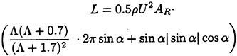
The resistance computed from the pressure field on the rudder is increased by
(1)
where T=propeller thrust, δ=rudder angle and Cth the thrust loading coefficient (Appendix 1). This expression is used if the vertical range of the rudder exceeds the propeller slipstream on both upper and lower ends; if not, the correction term is decreased appropriately. This corresponds to the assumption that the speed of the slipstream is not changed by the rudder, but that its direction follows the rudder midship plane, giving rise to a smaller longitudinal component of the propeller thrust.
Another influence of substituting the vortex transport equation by rot ![]() is an over-emphasis on the flow conditions just at the rudder surface while neglecting the conditions sideways from the rudder, which in reality influence rudder forces as well. To decrease this error, a weighted average of
is an over-emphasis on the flow conditions just at the rudder surface while neglecting the conditions sideways from the rudder, which in reality influence rudder forces as well. To decrease this error, a weighted average of ![]() along the transverse coordinate y is used:
along the transverse coordinate y is used:
(2)
Here c is the mean chord length of the rudder.
After these adaptations the forces produced by the panel method coincided much better with model measurements than without these measures.
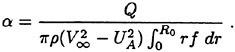
3.2 Estimation of propeller slipstream
The propeller slipstream is averaged in circumferential direction. Far behind the propeller, the axial velocity v(x, r) depending on longitudinal coordinate x (measured forward from the propeller plane) and on radius r is assumed as
(3)
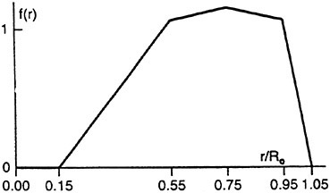
V∞ is the slipstream axial velocity far behind the propeller averaged over r, UA the uniform inflow velocity to the propeller. f(r) determines the radial thrust distribution; for the numerical examples it was assumed according to Fig. 2; R0 is the propeller radius. The nonzero values of f(r) beyond r/R0=1 are chosen to account for turbulent mixing of the propeller slipstream with the surrounding water. It was found that details of f(r) hardly influence the rudder force, but two things are important:
-
f(r) should gradually approach 0 at the outer limit;
-
f(r) should be zero in the hub region,
(a) avoids discontinuities of v at the outer slipstream radius, and (b) avoids very high circumferential velocities near the propeller axis; both features would degrade the accuracy of any point collocation method.
f(r) is scaled so that ![]() . Then V∞ can be determined from the thrust T, using the axial momentum equation, as
. Then V∞ can be determined from the thrust T, using the axial momentum equation, as
(4)
Further it is assumed that the ratio α between thrust Τ and propeller torque Q generated at any radius (and, thus, the efficiency of any ring of the propeller) is independent from r:
(5)
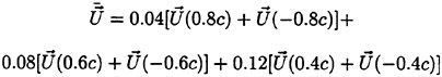
This allows to determine α and the circumferential velocity w at x=0 from the propeller torque Q as
(6)
Continuity gives the slipstream radius far behind the propeller as
(7)
For the slipstream contraction depending on x the relationship given in (3) was used:
(8)
with ξ=−x/R0. Continuity gives then the axial, circumferential and the radial velocity vr at finite x values for r<1.05R(x):
(9)
(10)
(11)
The partial derivative in the last equation is evaluated numerically.
From the axial, circumferential and radial velocity the Cartesian components of the inflow velocity ![]() are determined.
are determined.
3.3 Desingularized direct panel method
For lift-generating flows, direct panel methods, which use the flow potential as primary unknown, proved superior in accuracy to indirect methods, which use source and vortex strength as primary unknowns. Desingularized methods use singularities not on the body surface but inside the body, also to improve the accuracy for a given panel arrangement. The combination of desingularization with a direct method, which is used here, is—to my knowlegde—new. It solves the following equation, which may be derived from Green’s second identity applied to the potential ![]() of the flow disturbance
of the flow disturbance ![]() and to the Green function
and to the Green function ![]()
(12)
Here Sb and Sw designate body surfaces and wake sheets respectively. (The program is designed to handle several interacting bodies.) The right-hand side results from the condition of no flow through the body surfaces. ![]() designates points on the integration surface, whereas
designates points on the integration surface, whereas ![]() designates a finite number of collocation points inside the body or bodies near to the centres of each panel; the distance from the body surface is the smaller of the two values
designates a finite number of collocation points inside the body or bodies near to the centres of each panel; the distance from the body surface is the smaller of the two values ![]() and 1/3 · lokal thickness of the body. It turned out that the desingularization is more effective in simplifying the program than in improving the accuracy.
and 1/3 · lokal thickness of the body. It turned out that the desingularization is more effective in simplifying the program than in improving the accuracy.
The method handles only bodies with a sharp trailing edge; for finite end thickness, empirical corrections would appear necessary in any potential method. The shape of the wake sheet Sw is not computed, but assumed: Behind the trailing edge of each body a plane wake sheet in the direction δ/2 is assumed, and in the usual case of sharp upper and/or lower ends of the bodies, at the leeward knuckle line a wake sheet is assumed in the same direction, Fig. 3. The difference in ![]() on both sides of wake sheets is constant in flow direction, which is approximated here as the direction (cos(δ/2), sin(δ/2),0). Thus a subdivision of the wake sheets along this direction is not required; wake panels range from the trailing or upper or lower edge of the body all the way to the assumed aft end of the wake sheet at 20 c behind the body.
on both sides of wake sheets is constant in flow direction, which is approximated here as the direction (cos(δ/2), sin(δ/2),0). Thus a subdivision of the wake sheets along this direction is not required; wake panels range from the trailing or upper or lower edge of the body all the way to the assumed aft end of the wake sheet at 20 c behind the body.
In practice, the wake sheets wind up to concentrated end vortices. While this could, in principle, be modelled by a panel method, such a method would be complex and time-consuming, loosing much of the advantages of potential methods relative to Rans methods.
The integral ranges in (2) are subdivided into triangular and quadrilateral panels; the latter are approximated by two plane triangles forming a plane or meeting in a convex angle. Over each triangle the integrals are determined analytically. For the wake panels behind trailing edges, the difference of the potential on both sides of the wake is not a new unknown, but is equal to the difference of the potential between both sides of the body at the trailing edge. For the trailing edge potential, a linear extrapolation of the potential at the two panels immediately before the trailing edge on the same side of the body is used. In this way, each unknown wake potential difference is expressed as a linear combination of the (as well unknown) potentials on 4 body panels, resulting in a linear equations system having as unknowns only the body potentials. For the extrapolation, average panel potentials are assumed to be local potentials at the panel centres. This procedure avoids a) the inaccuracy which results if the wake potential difference is assumed to be equal to the potential difference between the last panels on both sides of the body, and b) the nonlinear equation system which results if equal pressure on both sides of the trailing edge is used as the end (Kutta) condition. For the wake panels starting at the upper and lower edge of the bodies, a simpler procedure is applied: Half of the potential difference between the panels immediately above the lower or below the upper edge is used as potential difference on both sides of these wake sheets.
3.4 Force and moment
To integrate force and moment we need the (average) pressure on each panel. The pressure follows from Bernoulli’s equation
(13)
![]() is the velocity on the same streamline far behind the body. That is not only difficult to determine; if we use
is the velocity on the same streamline far behind the body. That is not only difficult to determine; if we use ![]() and
and ![]() without taking account of the change of the wake and slipstream field by the rudder, results would be poor. Therefore the procedure sketched above (omitting the actual y coordinate and averaging over 5 different y values) is also here used to determine
without taking account of the change of the wake and slipstream field by the rudder, results would be poor. Therefore the procedure sketched above (omitting the actual y coordinate and averaging over 5 different y values) is also here used to determine ![]() and
and ![]() .
.
Different ways to determine ![]() from the
from the ![]() average over each panel were tried. The best method found was similar to that used, e.g., in (4) for propeller analysis: The average panel potentials are considered as local
average over each panel were tried. The best method found was similar to that used, e.g., in (4) for propeller analysis: The average panel potentials are considered as local ![]() values at the panel centres;
values at the panel centres; ![]() is interpolated by a quadratical polynomial over three adjacent panels both in longitudinal and vertical direction, giving the gradient times the direction vector for the respective interpolation; the
is interpolated by a quadratical polynomial over three adjacent panels both in longitudinal and vertical direction, giving the gradient times the direction vector for the respective interpolation; the ![]() component normal to the body surface follows from the body boundary condition; from the three (not all necessarily orthogonal) components of
component normal to the body surface follows from the body boundary condition; from the three (not all necessarily orthogonal) components of ![]() its Cartesian coordinates are determined. Whereas in most cases the neighbouring panels used for the interpolation lie on both sides of the panel P for which the gradient is to be determined, along the trailing, upper and lower edge of the bodies two panels on the same side of P have to be used. The pressure on the upper and lower face of the rudder, where not enough panels for the transverse interpolation are present, is neglected.
its Cartesian coordinates are determined. Whereas in most cases the neighbouring panels used for the interpolation lie on both sides of the panel P for which the gradient is to be determined, along the trailing, upper and lower edge of the bodies two panels on the same side of P have to be used. The pressure on the upper and lower face of the rudder, where not enough panels for the transverse interpolation are present, is neglected.
3.5 Further details
Rudders, fixed fins and end flaps are often separated from each other by small gaps of, say, 3–5 cm width. While gap widths of zero would result in a nearly or exactly singular equation system, gaps of 1 cm are handled without difficulties by the panel method. On the other hand, forces were found practically the same when gap widths were varied between 1 and 5 cm for typical full-scale rudder dimensions.
The effect of the hull above the rudder can be approximated by a horizontal mirror plane if it is not modelled as a separate body; also here a gap has to be provided in the calculation.
4 Single-blade rudder lift in uniform flow
In the following, rudder lift L and drag D are represented by non-dimensional lift and drag coefficients as usual:
(14)
v is the uniform inflow velocity, ρ the fluid density, AR the rudder area (projection on the xz plane). The stock moment M (relative to a given position measured from the profile nose) is represented by the moment coefficient
(15)
c is the (average) chord length. The rudder aspect ratio is defined as
(16)
b is the rudder height.
4.1 Lift gradient for moderate attack angles
According to potential theory, a thin foil in 2d flow (i.e. for Λ=∞) at a small angle of attack α produces lift nearly linearly increasing with α corresponding to
(17)
In 3d flow, the lift gradient is decreased by a reduction factor r(Λ) which is well approximated—compared to both theory and measurements—by
(18)
Except for Λ, details of the rudder shape in side view (e.g. rectangular, trapezoidal, elliptical) have hardly any influence on dCL/dα. However, the profile thickness and shape have some influence; e.g. Germanischer Lloyd assumes 20% larger forces for concave profiles.
Table 1 shows various results for dCL/dα corrected for infinite aspect ratio by using (18). The values resulted from measurements, potential calculations and Rans calculations for various profiles in 2d and 3d. The profile shapes are depicted in Fig. 4. The last 2 digits of the profile designation give the maximum profile thickness in % of c.
The following conclusions regarding dCL/dα corrected for Λ can be drawn:
-
All values differ from the theoretical value 2π by not more than ±17%.
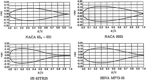
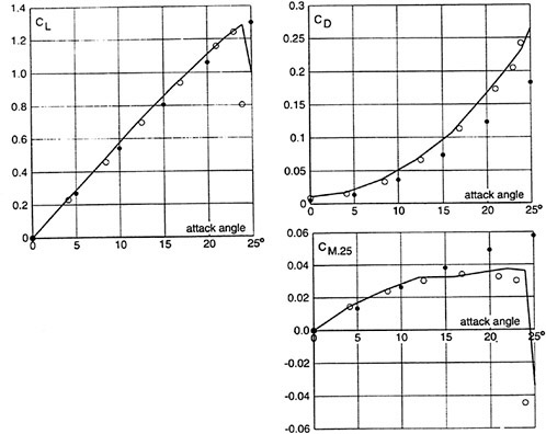
Table 1. Influence of profile shape and thickness on (dCL/dα)/r(Λ) “mod.” means: original profile modified to attain zero thickness at the trailing edge
|
Source |
Method |
Profile |
Λ |
Rn/106 |
(dCL/dα)/r(Λ) |
|
Abbott & Doenhoff 1959 |
Wind tunnel measurements |
NACA0006 NACA 634021 |
∞ ∞ |
9 9 |
6.30 6.78 |
|
Author |
Panel method |
NACA0006 NACA0025 IfS62 TR25 mod. HSVA MP73–25 mod. |
4 4 4 4 |
– – – – |
6.60 7.00 7.04 7.07 |
|
Chau 1997 |
Rans 2d |
NACA0025 IfS 62 TR 25 HSVA MP73–25 |
∞ ∞ ∞ |
6 6 6 |
5.25 6.40 6.40 |
|
Chau 1997 |
Rans 3d |
NACA0025 NACA0015 |
3 3 |
1.8 1.8 |
5.60 6.32 |
|
El Moctar |
Rans 2d |
NACA0025 IfS 62 TR 25 IfS 62 TR 25 mod. HSVA MP73–25 HSVA MP73–25 mod. |
∞ ∞ ∞ ∞ ∞ |
50 50 50 50 50 |
5.66 7.38 6.97 6.96 6.88 |
|
El Moctar |
Rans 3d |
NACA0025 IfS 62 TR 25 IfS 62 TR 25 mod. HSVA MP73–25 HSVA MP73–25 mod. |
4 4 4 4 4 |
50 50 50 50 50 |
6.47 7.35 7.15 7.03 7.08 |
|
El Moctar 1998 |
Rans 3d |
NACA0015 NACA0015 |
3 3 |
2.7 50 |
6.80 6.80 |
Table 2. Influence of profile thickness on CL(10°) due to 2D calculations for Rn=50 · 106 by El Moctar
|
Relative profile thickness t/c Profile type |
0.15 |
0.25 |
0.35 |
|||
|
CL |
CD |
CL |
CD |
CL |
CD |
|
|
NACA00xx |
1.02 |
0.016 |
0.91 |
0.016 |
0.72 |
0.018 |
|
HSVA MP73xx |
1.17 |
0.014 |
1.24 |
0.017 |
1.27 |
0.021 |
|
IfS62TRxx |
1.18 |
0.016 |
1.25 |
0.019 |
1.30 |
0.026 |
-
For the same profile, measurements and computations by any method differ generally by only a few percent; an exception is the relatively blunt NACA0025 profile.
-
2d and 3d Ranse calculations differ hardly from each other except for the NACA0025 profile.
-
The Reynolds number Rn=vc/ν has practically no effect (possibly except for the NACA0025 profile).
-
The low lift gradient of the relatively blunt NACA0025 profile is not correctly predicted by the panel method. (For such a profile, the end conditions used in potential flow are a very poor approximation.)
-
Finite thickness at the trailing edge increases the lift slope.
-
Ranse results by El Moctar are larger than those of Chau.
4.2 Effect of profile thickness
To investigate the effect of profile thickness in detail, El Moctar (personal communication) performed 2D RANSE calculations for the ΝACA00, IfS and HSVA profiles each for relative thickness 0.15, 0.25 and 0.35 with a very fine grid (105 cells). Thick profiles are required for rudders and other fins of high-speed vessels to accomodate the shaft, its coupling and/or bearing. The results for 10° angle of attack (Table 2) show:
-
Thick profiles produce more lift than thinner ones if they have a sharp end (concave sides),
-
and lower lift if they end in a larger angle (convex or flat sides).
-
The most-used NACA00 profiles are worse than the other profiles investigated, both with respect to lift slope and to the ratio between lift and drag; for 35% thickness, the NACA profile generates roughly 1/2 the lift only of the other profiles!
-
For all profiles, the lift/drag ratio decreases with increasing thickness. Thus, for a good propulsive efficiency, one should use the thinnest possible profile.
-
The IfS profile generates the largest lift; however, the difference to the HSVA profile is small, and the lift/drag ratio is worse than for the HSVA profile.
For a ship speed exceeding 23 knots, rudder cavitation could become a problem. In this respect the IfS profile with its very uneven pressure distribution on the suction side is especially prone to cavitation.
4.3 Maximum lift at stall angle
For increasing attack angle α, the lift coefficient rises up to a maximum CLmax at the stall angle, beyond which it decreases. At the maximum the CL(α) curve may be smooth or peaked, or two different values of CL may be possible in a range near αstall, depending on the profile shape and thickness.
Table 3. CLmax and αstall
|
Source |
Method |
Profile |
Λ |
Taper |
Rn/106 |
CLmax |
αstall |
|
Chau 1997 |
Rans 2d |
NACA0012 |
∞ |
– |
6 |
1.62 |
18 |
|
” |
” |
” |
” |
– |
60 |
1.63 |
18 |
|
Abbott&D. 1959 |
Wind tunnel |
” |
” |
– |
6 |
1.60 |
16 |
|
Chau 1997 |
Rans 2d |
NACA4412 |
∞ |
– |
6 |
1.91 |
18 |
|
Abbott&D. 1959 |
Wind tunnel |
” |
” |
– |
6 |
1.64 |
14 |
|
Chau 1997 |
Rans 2d |
NACA652–415 |
” |
– |
6 |
1.70 |
16 |
|
Abbott&D. 1959 |
Wind tunnel |
” |
” |
– |
6 |
1.55 |
18 |
|
Chau 1997 |
Rans 2d |
NACA0025 |
∞ |
– |
6 |
1.42 |
19 |
|
” |
” |
HSVA MP73–25 |
” |
– |
6 |
1.52 |
16 |
|
” |
” |
IfS 62 TR 25 |
” |
– |
6 |
1.34 |
13 |
|
Chau 1997 |
Rans 3d |
NACA0015 |
1 |
0.45 |
1.82 |
1.44 |
44 |
|
Whicker& Fehlner 1958 |
Wind tunnel |
” |
” |
” |
1.82 |
1.26 |
39 |
|
Chau 1997 |
Rans 3d |
NACA0015 |
2 |
” |
1.82 |
1.29 |
30 |
|
Whicker& Fehlner 1958 |
Wind tunnel |
” |
” |
” |
1.82 |
1.20 |
27 |
|
Chau 1997 |
Rans 3d |
NACA0015 |
3 |
” |
1.82 |
1.26 |
25 |
|
Whicker& Fehlner 1958 |
Wind tunnel |
” |
” |
” |
1.82 |
1.15 |
23 |
|
Chau 1997 |
Rans 3d |
NACA0015 |
3 |
” |
18.2 |
1.37 |
27 |
|
Whicker& Fehlner 1958 |
Wind tunnel |
” |
” |
” |
18.2 |
1.25 |
23 |
|
Chau 1997 |
Rans 3d |
NACA0025 |
1 |
1.0 |
0.78 |
1.30 |
42 |
|
Thieme 1962 |
Wind tunnel |
” |
” |
” |
” |
1.34 |
46 |
|
Thieme 1962 |
Wind tunnel |
NACA0015 |
” |
” |
” |
1.06 |
34 |
|
Chau 1997 |
Rans 3d |
HSVA MP73–25 |
” |
” |
” |
1.42 |
44 |
|
” |
” |
IfS 62 TR 25 |
” |
” |
” |
1.19 |
37 |
|
Thieme 1962 |
Wind tunnel |
” |
” |
” |
” |
1.47 |
46 |
|
Chau 1997 |
Rans 3d |
NACA0015 |
3 |
0.45 |
1.82 |
1.26 |
25 |
|
” |
” |
” |
” |
1.0 |
1.82 |
1.26 |
25 |
|
El Moctar |
Rans 2d |
IfS 62 TR 25 |
∞ |
– |
50 |
2.11 |
18 |
|
” |
” |
HSVA MP73–25 |
” |
– |
” |
2.06 |
21 |
|
” |
” |
NACA0025 |
” |
– |
” |
1.88 |
23 |
|
El Moctar 1998 |
Rans 3d |
IfS 62 TR 25 |
4 |
1.0 |
50 |
2.05 |
31 |
|
” |
” |
HSVA MP73–25 |
” |
” |
” |
1.96 |
35 |
|
” |
” |
NACA0025 |
” |
” |
” |
1.74 |
33 |
|
El Moctar 1998 |
Rans 3d |
NACA0015 |
1 |
0.45 |
2.7 |
1.29 |
45 |
|
” |
” |
NACA0015 |
3 |
” |
” |
1.29 |
27 |
|
Whicker& Fehlner 1958 |
Wind tunnel |
” |
” |
” |
” |
1.24 |
23 |
|
El Moctar 1998 |
Rans 3d |
” |
” |
” |
50 |
1.48 |
27 |
At stall condition the flow separation point on the suction side changes, gradually or suddenly, from the aft to the front part of the foil. (For α<αstall a short laminar separation bubble may occur in the front part of the profile suction side; it has hardly any influence on lift.) For hard-over rudder manoeuvres, the lift maximum may be more important than dCL/dα.
Table 3 gives computed and measured values from various sources. Because stall is a viscous phenomenon, no computations using the panel method are included. The following conclusions can be drawn from Table 3:
-
For Rn>0.8·106, CLmax varies in a wide range between about 1.2 and 2. This upper limit is substantially larger than assumed in classification rules.
-
The aspect ratio is of minor influence only: larger aspect ratio produces somewhat smaller CLmax.
-
Contrary to the above statement, 2d calculations give 3 to 7% larger CLmax values than 3d calculations for Λ=4.
-
The strong dependence of dCL/dα. on Λ and the weak dependence of CLmax on Λ result in a strong dependence of αstall on Λ: Small Λ gives large αstall.
-
Higher Reynolds numbers produce larger CLmax also beyond the experimental range of about 3 · 106, at least in 3d calculations and measurements; thus experimental values alone, without extrapolation to actual Rn, are misleading with respect to CLmax.
-
The taper ratio has practically no influence on CLmax.
-
Larger profile thickness gives larger CLmax.
-
Some of the values computed by Chau deviate a little from the measured values to both sides, while the results of El Moctar closely correspond to the comparable measurements; however, both authors dealt with different cases, so that definite conclusions would be premature.
-
Profiles with concave sides produce larger CLmax than those with flat or convex sides.
The relation between 2d and 3d values of CLmax allows to approximately determine the maximum lift while avoiding the complexities of 3d Rans calculations especially for complex configurations and non-uniform inflow: Perform a 2d Rans calculation for the actual profile and Rn in uniform flow to determine CLmax,2d; perform a panel calculation for the 3d arrangement; convert the computed lift to CL using an average inflow velocity; determine the approximate stall angle as that where the 3d CL in potential flow amounts to 95% of CLmax,2d; truncate the computed forces and moment at that angle. The velocity average used in this procedure is the root mean square velocity (x component of ![]() in eq. 1) averaged over the rudder surface.—Beyond the stall angle also Rans calculations give only a rough indication of the real forces.
in eq. 1) averaged over the rudder surface.—Beyond the stall angle also Rans calculations give only a rough indication of the real forces.
5 Single-blade rudder drag and stock moment in uniform stream
Whicker and Fehlner (6) measured forces on a trapezoidal rudder (lower c/upper c=0.45) with a NACA0015 profile and a geometric aspect ratio of 1.5 for Rn≈1.8 · 106; at the upper end of the rudder a large horizontal plate was attached with a very small gap, resulting in an effective aspect ratio of 3. Fig. 5 compares their measured results (○) for lift, drag and stock moment with Rans calculations by El Moctar (lines) and own panel calculations (●). All the lift data show very good coincidence; the same holds for the measured and Rans-computed drag and stock moment. The drag computed by the panel method is about 25% too small, whereas the panel stock moment indicates a point of attack of the transverse force which, for 20° rudder angle, lies about 1.5% of c in front of the measured one. Because no viscous corrections were made for the drag, the small non-zero value at 0° indicates the discretization error.
6 Forces on rudders behind ship hull and propeller
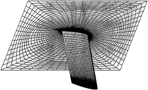
Fig. 6 shows the propeller and rudder arrangement for a ship of Flensburger Schiffbau Gesellschaft (FSG) for which model experiments were conducted in the Potsdam towing tank (SVA). In the self-propulsion tests also rudder forces and rudder stock moment were measured while the model was forced to run straight ahead. The rudder is arranged below a fixed fin. In way of the propeller hub a Costa bulb is arranged.
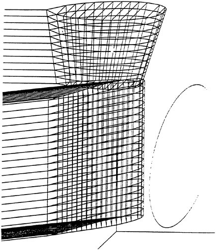
For such complicated arrangements, Ranse calculations have not yet been performed. Thus Fig. 7 compares the measured data (○) only with results of the panel method (lines). The panel arrangement used and the velocity vectors at panel centres for one case are shown in Fig. 8. Instead of the hull above the fixed fin, a horizontal mirror plane was arranged in the calculation. The ship wake was assumed uniform, corresponding to the effective wake
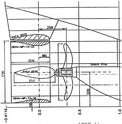
Fig. 6. Rudder arrangement of FSG ship
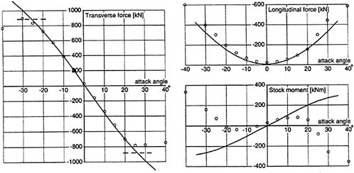
Fig. 7. Forces and moments on the rudder of Fig. 6. ○: measurements of SVA Potsdam; curves: panel method results; broken line: extreme lift estimated from 2D RANS results
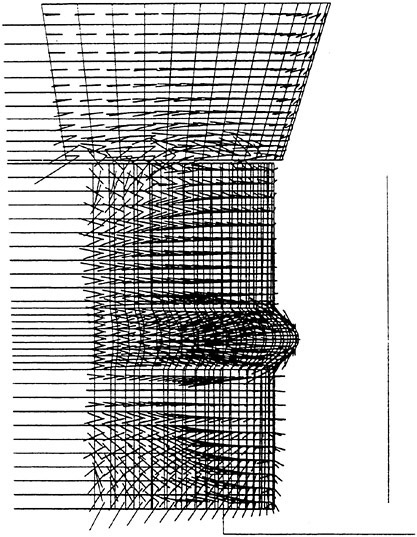
Fig. 8. Panel arrangement corr. to Fig. 6 for 35° rudder angle and computed velocity vectors. The vertical line in front of the rudder is the propeller disc
at the propeller. Due to the non-uniform inflow produced by the propeller, results differ a little between port and starboard rudder. As to the stock moment, for small rudder angle an error of about 3% of c (computed attack point forward of measured one) is found, whereas for −20° the error increases to about 8% of c; thus the moment error is here larger than in free stream. The reason is, presumably, also the fundamental error of underestimating the interaction between the propeller slipstream and the flow induced by the rudder: The wakes at the top and bottom edges of the rudder, which are effective in shifting the attack point of the transverse force backward, were relatively weak in the computation because upper and lower end of the rudder were outside of the propeller slipstream; in reality, however, the propeller slipstream is elongated in vertical direction by the rudder at the aft end of the pressure side due to the vertical rudder-induced velocities.
For the Reynolds number Rn=0.26 · 106 of the experiments, 2D RANSE calculations in uniform flow gave CLmax=1.24. Corresponding to the procedure scetched in section 4.3, the maximum lift in 3D flow is estmated as ±884 kN (broken lines in CL diagram, Fig. 7). This corresponds closely to the measured extreme transverse force. On the other hand, due to the different Rn the full-scale maximum lift coefficient, estimated in the same way, is about 70% larger.
7 Approximation of the transverse force of a rudder behind a propeller
The lift of a rudder of area AR in free flow conditions for attack angles α<αstall is well approximated by
(19)
In the appendix the additional lift of a rudder behind a propeller is estimated roughly as
(20)
This is used here as a basis for a more accurate prediction by introducing two corrections:
-
If, in vertical direction, the rudder is asymmetrical with respect to the propeller axis, the twist of the propeller slipstream generates a non-zero rudder angle δ0 for which the lift is zero.
-
In the appendix it was assumed that the flow behind the propeller is deflected laterally by an angle equal to the rudder angle δ. This assumption is modified here by introducing a correction factor C.
Thus the additional rudder lift due to the propeller is approximated by
(21)
The dependence on Cth is illustrated in Fig. 9.
By applying the panel program for various propeller loadings and ratios between propeller diameter D, rudder chord length, rudder height, height of propeller axis and longitudinal distance between propeller and rudder, C was determined for many different arrangements. Results showed that C depends primarily on the difference in height between upper end of the rudder and top of the propeller circle, htop, and between the bottom of the propeller circle and the base point of the rudder, hbottom:
(22)
Fig. 10 shows an average curve for fC found in these calculations, together with an illustration of the factor ![]() in eq. 21.
in eq. 21.
Manufacturers of steerable propulsors like waterjets, “azipots”, “pumpjets” etc. often claim better steering performance of ships with these “active” steering devices than attained by a usual “passive” rudder. Practical experience, however, is often to the contrary. This is explained by eq. 21: The side force produced by these usually highly loaded propulsors is, with good approximation, equal to T sin δ, where δ is the turning angle of the propulsor. For a rudder behind the propeller, however, eq. 21 gives, typically, a side force of about 1.4T sin δ due to the propeller action, and additionally 1/2 to 1/3 of that value due to the rudder without propeller; thus, in sum a rudder behind a usual propeller generates, roughly, 2T sin δ, i.e. twice the lateral force for an “active”, steerable propulsor. This explains partly the difficulties (slow turning response; large yaw and heavy speed loss in waves) which have often been encountered in ships with such types of propulsors if they do not have a rudder. (Another problem may be yaw instability due to lacking skeg area in the afterbody.)
8 Practical consequences
For a turning ship, except at the start of the turn rudder angles of attack α are much smaller
than the rudder angle δ relative to the midship plane. Comparing these small attack angles with the large stall angles of Table 3 for full-scale Rn, it is obvious that larger maximum rudder angles than the usual 35° are a simple, cost-efficient means of improving the turning ability of ships.
However, in yaw checking large rudder angles opposite to the turning motion would lead to stall and the accompanied decrease of rudder transverse force. This is easily avoided by limiting the shaft moment which the rudder gear can generate to about the stall angle moment; then in yaw checking the rudder will just operate at the stall angle, producing maximum lift. This better manoeuvring for smaller maximum rudder gear moment was also observed practically by FSG on trial trips. For large ships this may result in difficulties to satisfy the IMO requirement of turning the rudder, at full ship speed, within 28s from 35° on one side to 30° on the other side. This rule, which is criticized also because the 28s limit should better depend on ship size and speed, should be substituted.
As demonstrated in Tables 1 to 3, to generate large lift (both for fixed α and maximum lift), rudders should have concave profiles with small or zero trailing edge angle. This holds especially for thicker profiles of, say, 20 to 25% c. The now most used NACA00xx profiles should be avoided, especially in thick profiles.
Thicker profiles generate both larger lift gradient and larger maximum lift. The lift/drag ratio, however, is worse than for thinner profiles.
Finite end thickness of rudder profiles increases the lift, but also the drag; therefore thin profile ends should be preferred. For hollow profiles this results in structural difficulties if the usual rudder construction ending in 3 plates (a middle plate and two outer skin plates) is used. An asymmetrical structure as scetched in Fig. 11 may be better; however this requires some care to avoid asymmetrical deformations due to weld shrinking, or to use these deformations intentionally to adapt the rudder to the propeller slipstream twist.
For higher speed exceeding, say, 23 knots, rudder cavitation even at small or zero rudder angle may become a problem especially for thick rudders and highly loaded, slow running propellers. The panel method is an easy and, presumably, reliable means to determine whether zero absolute pressure (which is, in full scale, not far from the cavitation limit) occurs. If problems are expected, special symmetrical profile shapes (7) or unsymmetrical profiles adapted to the propeller slipstream may be used as a remedy, and their effect predicted by a panel method. Whether such profiles can provide also better propulsive efficiency is not yet clear.
To decrease scale effects in manoeuvring model experiments, the maximum lift coefficient of the model rudder should be increased. A way to do this is to use a flap rudder in the model instead of a non-flapped rudder in the ship. The flap (area and angle) should be designed such as to produce the same maximum lift coefficient in model conditions as the ship rudder is expected to produce in full-scale conditions. To compensate for the larger dCL/dα of the model flap rudder, the model rudder angles should be decreased appropriately.
References
1. Chau, S.-W., “Computation of rudder force and moment in uniform flow”, Ship Techn. Res. Vol. 45 No. 1, pp. 3–13
2. El Moctar, O.A.M., “Numerical determination of rudder forces”, Euromech 374 (1998), Poitiers
3. Söding, H. “Forces on rudders behind a maneuvering ship”, 3rd Int. Conf. Num. Ship Hydrodyn. (1981), Paris
4. Lee, J.-T., “A potential based panel method for the analysis of marine propellers in steady flow”, Rep. 87–13, Dept. of Ocean Eng., MIT
5. Abbott, I. and Doenhoff, A., Theory of wing sections, Dover Publ., New York 1959
6. Whicker, L.F. and Fehlner, L.F., “Freestream characteristics of a family of low-aspect-ratio, all-movable control surfaces for application to ship design”, Rep. 933 (1958) David Taylor Model Basin
7. Brix, J., Manoeuvring Technical Manual, Seehafen Verlag 1993, ISBN 3–87743–902–0
8. Chau, S.-W. “Numerical investigation of free-stream rudder characteristics using a multi-block finite volume method”, Rep. 560, 1997, Institut für Schiffbau, Hamburg
9. Thieme, H., “Zur Formgebung von Schiffsrudern”, Jahrbuch Schiffbautechn. Gesellschaft 1962, Springer
Appendix: Momentum of propeller-rudder flow
The additional lift and drag produced by a rudder due to a propeller in front of it will be estimated roughly by momentum theory. To that end, a circular cylinder of propeller diameter (cross section area Ap=πD2/4) is considered, initially for rudder angle zero. It is assumed that outside of this cylinder the flow speed is not changed by the propeller.
Due to propeller slipstream contraction, the cylinder surface is not a streamline surface. Neglecting turbulent mixing, far behind the propeller the cylinder contains an inner region where the fluid velocity is ![]() according to the propeller momentum theory; in the outer cylinder region the fluid velocity is assumed to be U, the inflow speed to the propeller. Cth=T/0.5ρU2Ap is the thrust loading coefficient of the propeller. In the propeller plane, the longitudinal flow speed is the average between U and
according to the propeller momentum theory; in the outer cylinder region the fluid velocity is assumed to be U, the inflow speed to the propeller. Cth=T/0.5ρU2Ap is the thrust loading coefficient of the propeller. In the propeller plane, the longitudinal flow speed is the average between U and ![]() . Continuity requires that the inner and outer cross section areas are
. Continuity requires that the inner and outer cross section areas are
(23)
respectively.
Compared to the flow without propeller loading, the flow of longitudinal momentum at the cylinder outlet is increased by
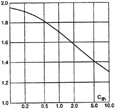
Fig. 9. Function ![]() of eq. 21
of eq. 21
(24)
Inserting here the above relations gives the momentum flow increase as
(25)
For a very lightly loaded propeller this momentum flow increase is twice the propeller thrust, whereas for a heavily loaded propeller it is equal to T. The excess over Τ is caused by the fact that the contraction of the propeller slipstream causes more water to pass the cylinder then without the propeller.
If the rudder is deflected by the angle δ, a first approximation is that also the streamlines within the considered cylinder are deflected laterally by δ whereas the modulus of the flow speed remains unchanged in the average. Compared to the rudder without propeller loading, the rudder behind the propeller generates then an additional transverse thrust of
(26)
and an increase in resistance (or decrease in propeller thrust) of
(27)
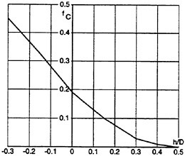
Fig. 10. fC(h) of eq. 22
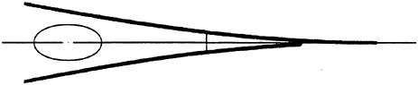
Fig. 11. Proposed aft end structure of a rudder
DISCUSSION
D.Clarke
University of Newcastle Upon Tyne, United Kingdom
I would like to add my congratulations to Professor Söding for a clear and interesting presentation. I am in complete agreement with his approach to modeling this complex subject, which is to keep it as simple as possible, whilst still accounting for all known influences. Professor Söding blames the IMO for the rule concerning the rudder rate of travel, but I rather think that this comes directly as a requirement in Lloyd’s Rules. It is more concerned with the strength of the rudder stock and the capability of the steering gear than with maneuvering.
I notice that he uses a lift reduction coefficient, which appears in Eq. 19 of his paper. This appears somewhat different to the classical Prandtl lifting line correction, so could he please explain on what grounds he added the extra terms?
Finally, could I ask Professor Söding if he has considered plotting his results in the form of interference factors, so that the basic lift on the rudder may be modified to account for the free surface mirror effect, area ratio of fixed to moving parts, and fixed horn at the leading edge of the rudder?
Thank you for a very interesting paper.
AUTHOR’S REPLY
The lift reduction due to aspect ratio Λ in eq. 19 was chosen to converge Λ/4 for Λ→0, to 1 for Λ→∞, and to correspond, between these limits, closely to numerical results of the lifting-surface theory. For most of the influences for which Prof. Clarke asked, results, mostly from 2D calculations, are given in [3]. But due to the many possible arrangements and the small effort in performing a calculation, today I prefer to compute each case when it comes up.
DISCUSSION
G.Hearn
University of Newcastle Upon Tyne, United Kingdom
Thank you for a lecture full of insight, and for fulfilling your aim of good engineering. In an earlier comment by my colleague, Dr. Clarke, the subject of interference factors was raised. In work carried out with my colleague the interference factor associated with aeroplane tail fins was applied to the double ship model with skeg by rotating the aero analysis through 90 degrees and then taking into account the existence of port and starboard vortices. Such an approach was sufficient (see references) to remove the difference between the usual potential theory based predictions of longitudinal hull forces and measured forces for a maneuvering ship, getting reasonable results over the latter (aft) 25% of ship length being the challenge. The existence of such vortices would also influence the force experienced by the rudder. Do you intend to include this influence?
Refer to [1] MARSIM ’93 and [2] 18th ONR Symposium on Naval Hydrodynamics.
AUTHOR’S REPLY
Regarding hull forces in maneuvering, I combine slender lifting body theory [7] with cross-flow resistance coefficients chosen to obtain correspondence of simulated with trial trip results. Current work is in combining hull, rudder, and propeller (the latter modeled by volume forces) in Ranse calculations similar to the work described by Cura Hochbaum in this conference.
DISCUSSION
A.Graham
Department of National Defence, Canada
Firstly, may I thank the author for an interesting paper, one of practical interest to engineers. The conclusions remind me of some design studies I was involved in just a few years ago when we were investigating the Schilling rudder concept. For those of you not familiar with this concept it is a fish-tailed rudder with end plates able to swing between 70° port and 70° starboard. It allows a vessel to dispense with a stern thruster. The Schilling rudder generates huge side thrust and makes for a very effective slow-speed maneuvering aid. I wondered if the author has yet considered this concept in his studies?
AUTHOR’S REPLY
My collaborators and I have not yet investigated Schilling rudders. Certainly potential flow
methods, and probably also stationary Ranse methods, are not suitable to handle the Schilling rudder profile with its thick trailing edge, and the very large rudder angles used typically in these designs, because both features lead to massive flow separation which is not covered correctly by the κ-ε turbulence model and gives rise to instationary flow.
DISCUSSION
A.Reed
Naval Surface Warfare Center
Carderock Division, USA
I have two questions for Prof. Söding. First, could he please comment further on the modeling of the wake behind the rudder—does the wake plane remain parallel to the rudder plane to “infinity” and if so, what are the effects of the free stream flow across the wake sheet on the accuracy of the force calculations?
Second, could he provide some details on the methods used to model the propeller in the potential flow model of the hull, propeller, and rudder?
AUTHOR’S REPLY
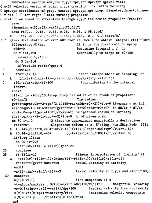
The rudder wake was assumed as a plane from trailing edge to nearly infinity, having a direction averaged between the rudder plane and the inflow direction. This is the typical assumption in classical airfoil theory. The wake direction influences the (small) nonlinear part of the L(α) curve. To include the vortex rollup in the rudder wake would give a better distribution of lift over span, but it has hardly any effect on total lift. The details of the propeller slipstream assessment are discribed in the Fortran77 program given below.
DISCUSSION
K.Nakatake
Kyushu University, Japan
Thank you very much for your paper of practical importance. I wish to make a small comment. I have been working in the field of resistance and propulsion theory and I think our group could verify the mechanism of hull-propeller-rudder interaction. From our experience, the propeller model seems to be too simple. The propeller model should express the accelerated flow and the rotating flow in the propeller race. I expect that more exact models such as “the simplified propeller model” will be introduced into the maneuvering field. Thanks for your attention.
AUTHORS’ REPLY
My propeller slipstream model takes into account the axially accelerated and rotating flow. To me, circumferential averaging seems plausible if we are interested not in vibrations, but in time-averaged rudder forces relevant for maneuvering predictions. Thus, inaccuracies of the propeller model are expected to be due mostly to the radial distribution of the propeller load. If this distribution is known, it can be applied in my procedure (see program below). In my view, to have a better propeller model may make sense for very accurate viscous rudder flow calculations, but not for potential flow methods with their intrinsically larger errors. More important error sources in rudder forces influenced by hull and propeller are probably the turbulent mixing of the propeller slipstream with the surrounding fluid, the flow acceleration with increasing distance from the stern due to the hull displacement effect, and the flow curvature behind a drifting or turning ship hull.
I thank all the discussers for their encouragement and valuable comments. Please see the Fortran77 program mentioned above on the following page.