A Two-Fluid Navier-Stokes Solver to Simulate Water Entry
S.Muzaferija, M.Peric (Technical University of Hamburg-Harburg, Germany)
P.Sames, T.Schellin (Germanischer Lloyd AG, Germany)
Abstract
Viscous free-surface flows associated with water entry were predicted by a finite volume method incorporating a free-surface capturing model. The method was applied to simulate two- and three-dimensional water entry processes, obtaining favorable agreement with measurements.
1 Introduction
Simulation of water entry phenomena requires accounting for the irregular deformation of the free surface, including splashing and breaking of waves. Of the methods available today to compute free-surface flows, interface-tracking methods (1,2) use interface-fitted moving grids, and interface-capturing methods (3–7) use fixed grids and solve an additional equation to locate the free surface. It is impractical to apply interface-tracking methods to simulate water entry problems such as slamming because the grid has to be adapted both to the free surface and to the shape of the entering body. Additionally, the free surface can change its topology due to wave breaking, overturning or splashing. This inevitably causes the grid to deform to such an extent that re-gridding becomes necessary. On the other hand, interface-capturing methods can be applied to arbitrary water entry processes because the application of these methods is not restricted to smooth free surfaces. The classical volume-of-fluid (VOF) (3) and marker-in-cell (MAC) (4) methods are examples of interface capturing methods that solve the Navier-Stokes equations for one fluid only. Recently developed methods that compute the flow of two fluids are the density function method (5) and the two-fluid models of Lafaurie et al. (6), Ubbink (7) and Muzaferija and Perić (8).
We demonstrated the applicability of the latter method (8) to water entry problems. Two fluids, air and water, are considered a single continuum with variable properties. An additional transport equation for the void fraction of one of the fluids is solved to determine the spatial distribution of the two fluids, and a special discretization scheme for the convective fluxes in the void fraction transport equation is used to achieve a sharp interface between the two fluids and to ensure void fractions bounded between zero and unity.
Investigating water entry of flared ships sections, Arai et al. (9) applied a two-dimensional finite difference method to solve the Euler equations and a VOF algorithm to capture arbitrary free-surface deformations. They showed that splash significantly affects predicted pressures at ship bow sections and, therefore, must be accounted for. Applying a potential flow based boundary element method to slamming for three-dimensional geometries, Troesch and Kang (10) found that small roll angles significantly reduce the bottom impact pressures whereas the flare impact pressures remained unaffected. Therefore, model tests must be conducted carefully to accu-
rately account for all important parameters that may influence results. Zhao et al. (11) applied a two-dimensional method that accounts for splash effects to the water entry of a wedge and a flared ship section. For the ship section, numerical pressure predictions compared favorably with model test measurements. For the wedge, pressures were overpredicted, and significant three-dimensional effects were shown to be important. Schumann (12) used a finite volume method with a VOF approach to capture the free surface. He investigated bow flare slamming phenomena for different flare angles. Sames et al. (13) presented a complete slamming analysis, including ship motion perditions and water entry simulations. They found that the motion history of water entry significantly affected predicted pressures.
We computed water entry processes for a flared ship section and a wedge and compared numerical results with measurements. Our systematic two- and three-dimensional computations assessed the influence of initial and boundary conditions.
2 Solution Method
The conservation equations of mass, volume concentrations and momentum describe the behavior of a multi-fluid system:
(1)
(2)
(3)
Here, V is an arbitrary control volume bounded by a closed surface S, ρ is the density, v is the fluid velocity vector, n is the unit vector normal to the surface S and directed outwards, ci is the volume concentration of the ith fluid component, T is the stress tensor, and fb is the resultant body force. For Newtonian incompressible fluids considered here the stress tensor is related to the rate of strain tensor via Stokes’ law:
(4)
where D is the rate of strain tensor, μ is the dynamic viscosity, p is the pressure, and I is the unit tensor.
The conservation equations of the volume concentration of each fluid component are another form of the mass conservation equation; their sum equals the overall mass conservation equation (1).
The mixture of fluids is treated as a single effective fluid, whose physical properties can be expressed as a function of the volume concentrations and the physical properties of each fluid component:
(5)
where ρi and μi are the density and viscosity of the ith fluid component, respectively.
In order to solve the governing equations, the solution domain is first subdivided into an arbitrary number of contiguous control volumes (CVs) or cells. Control volumes can be of an arbitrary polyhedral shape (see Fig. 1) allowing for local grid refinement, sliding grids, and block-structured grids with non-matching block interfaces. This simplifies grid generation and enables a more effective distribution of grid points by clustering them in the regions of strong variation of variables. The values of all dependent variables are stored in the center of each CV. The

Figure 1: Polyhedral control volume.
governing equations are integrated over each CV. The volume and surface integrals are calculated using second-order approximations (linear interpolation, central differences, and midpoint rule integration). The method is fully implicit, i.e., the spatial integrals are evaluated at the new time level while the old values appear only in the approximations of the time derivative (linear or quadratic backward scheme). The pressure-correction equation derived from the discretized continuity and momentum equations (14) is used to determine the pressure. Two-equation models belonging to the k-∈ family yield the eddy viscosity in case of turbulent flow computations. The resulting system of nonlinear and coupled algebraic equations is solved iteratively in a sequential manner. The linearized equations are solved using solvers from the family of conjugate-gradient methods. Iterations are repeated within each time step
until the nonlinear equations are satisfied within acceptable tolerances. More details about this finite-volume FV discretization can be found in (14). Here only the interface-capturing features of the method will be discussed.
The discretization of the convective part of the volume fraction conservation equation needs special attention. Ideally, its discretization should neither produce numerical diffusion nor unbounded values of the volume fraction, i.e. the value of the volume fraction in each cell should lie between the minimum and maximum value of the neighbor cells. The demand for a scheme to be bounded implies that the computed fluxes of volume fraction do not underflow or overflow the cells.
The numerical diffusion is associated with the first-order upwind scheme (UD) that approximates the cell face value by the value at the upstream cell center (Fig. 2). It is unconditionally stable and always produces a bounded solution. On the other hand, the downwind scheme (DD) is an unconditionally unstable first-order scheme that introduces negative numerical diffusion. It approximates the cell face value by the value at the downstream cell center. This discretization will try to recover a sharp interface even if some smearing of the volume fraction takes place. Both schemes have desirable properties; they are simple and involve only nearest neighbors, and they yield the correct speed of the interface under the assumption that the interface remains sharp and nearly flat. These two schemes have properties that can be combined to yield a discretization that is both bounded and free (or almost free) of numerical diffusion.
The way of blending UD and DD can be analyzed in the Normalized Variable Diagram (NVD) (8). The local normalized volume fraction ![]() in the vicinity of the cell center C is defined as follows:
in the vicinity of the cell center C is defined as follows:
(6)
where subscripts U and D denote the respective nodes upstream and downstream of the cell center C (Fig. 2), and r is the position vector.
If the discretization yields a value of the normalized volume fraction ![]() at the cell face j that lies inside the shaded region of the normalized variable diagram (Fig. 3) or along the diagonal
at the cell face j that lies inside the shaded region of the normalized variable diagram (Fig. 3) or along the diagonal ![]() a bounded solution at the cell center will be obtained. The diagonal
a bounded solution at the cell center will be obtained. The diagonal ![]() corresponds to the upwind discretization. Only the upwind discretization produces a bounded solution for values of
corresponds to the upwind discretization. Only the upwind discretization produces a bounded solution for values of ![]() smaller than 0 and larger than 1. In the region
smaller than 0 and larger than 1. In the region ![]() many combinations of UD and DD will give bounded solu
many combinations of UD and DD will give bounded solu
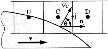
Figure 2: Notation and values used for NVD diagram and HRIC scheme.
tions. Our aim is to find one which produces both sharp interfaces and bounded solutions.
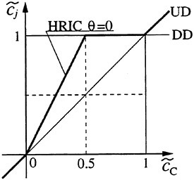
Figure 3: Normalized variable diagram and the HRIC scheme.
For ![]() UD and DD yield the same face value of
UD and DD yield the same face value of ![]() so the switching from DD to UD can be done continuously. However, for the value
so the switching from DD to UD can be done continuously. However, for the value ![]() UD and DD result in values of either 0 or 1 for
UD and DD result in values of either 0 or 1 for ![]() . For a sudden switch from UD to DD the resulting discretization is unstable because small changes of
. For a sudden switch from UD to DD the resulting discretization is unstable because small changes of ![]() cause large changes of
cause large changes of ![]() . Therefore, a gradual change from downwinding to upwinding is necessary.
. Therefore, a gradual change from downwinding to upwinding is necessary.
We used the High Resolution Interface Capturing (HRIC) scheme to compute the cell face value of the volume fraction according to the following expression:
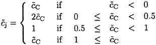
(7)
Figure 3 shows a graphical interpretation of this scheme.
Downwind discretization may cause an alignment of the interface with the numerical grid (7). To prevent this alignment, the discretization has to account for the angle θ between the normal to the interface
(defined by the gradient of the volume fraction ∇c) and the normal to the cell face (Fig. 2). The HRIC scheme corrects the ![]() value according to the following expression:
value according to the following expression:
(8)
The blending of upwind and downwind schemes is dynamic and accounts for the local distribution of the volume fraction. However, if the local Courant number Co,
(9)
is too large, the dynamic nature of the scheme may cause convergence problems. To prevent this, the HRIC discretization also takes into account the value of Co, yielding the cell-face value of the volume fraction according to the following expression:
(10)
Finally, the cell-face value of c is computed according to Eq. (6) as follows:
(11)
where the blending factor γ is defined as:
(12)
The discretizations used in the SURFER code (6) as well as in the CICSAM scheme of Ubbink (7) have components similar to those used to construct the HRIC scheme. A successful scheme for interface capturing must exploit the interface sharpening nature of the downwind scheme, it must prevent over-and underflow of cells (it has to be bounded), and it should have a mechanism to avoid alignment of the interface with the numerical grid.
The solution procedure follows the well known SIMPLE algorithm for pressure velocity coupling and can be summarized as follows (8,14):
-
Initialize all variables at initial time t0.
-
Advance time to tk=tk−1+Δt.
-
Update the coefficients of the momentum equations and solve the linearized system to obtain an improved estimate of the velocity.
-
Calculate new mass fluxes, solve the pressure correction equation, and correct mass fluxes, cell center velocities, and pressures.
-
Solve transport equations for volume fractions and update fluid properties.
-
If necessary, solve additional conservation equations (energy, turbulence quantities, etc.).
-
If the convergence criterion for the current time step is satisfied, increase the time step counter k and go to step 2. If not, return to step 3.
The calculation stops after reaching the maximum prescribed number of time steps.
3 Results and discussion
We systematically applied the new computational method to simulate water entry phenomena. Two-dimensional simulations of water entry of a flared ship section and two- as well as three-dimensional simulations of water entry of a wedge were compared with experimental data of Zhao et al. (11). We assumed laminar and incompressible flow and treated the ship section and the wedge as rigid bodies. Motion histories of water entries given in (11) were prescribed for the simulations performed with constant time steps. Time t=0 s corresponded to the impact of the body with the initially undisturbed free surface. We started the simulations with the water level well below the keel.
3.1 Flared ship section
3.1.1 Effect of refining in space and time
We generated two-dimensional grids and successively refined them by repeated subdivision of each grid cell to study effects of cell size. Figure 4 shows the coarse grid with 775 control volumes (CVs). The complete computational domain is visible. We applied a no-slip boundary condition at the section contour, a symmetry boundary condition at the left of the domain, a slip wall boundary condition at the right of the domain, an inlet boundary condition with prescribed velocities at the lower side of the domain, and a pressure boundary condition at the upper side of the domain. The grid comprised five independently created blocks. The inner block adjacent to the ship’s side contained ny·nz CVs. Here ny denotes the number of CVs in the direction tangential to the body contour and nz the number of CVs in the normal direction. Another block was arranged above this inner block to account for the splash. A third block with a non-matching interface was located above the deck. Adjacent and below the inner block two blocks were arranged, again with non-matching interfaces
towards the inner block. Figure 5 shows a partial view of the medium grid with 3100 CVs. Figure 6 shows a close-up view of the fine grid with 11200 CVs.
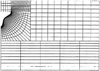
Figure 4: Computational grid with 775 CVs.
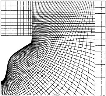
Figure 5: Partial view of computational grid with 3100 CVs.
We performed two sets of computations. Table 1 lists main particulars of simulations performed: total number of CVs, number of CVs in the inner block, time step size Δt, and width of grid cell at the body surface Δn.
The first set of computations employed three grids with 775, 3100 and 11200 CVs. Figure 7 shows time series of predicted vertical force Fz during water entry including measurements. Numerical results showed that the 775 CVs grid was not sufficiently fine to capture the maximum vertical force. The other two solutions based on the 3100 CVs and the 11200 CVs grids agreed favorably with measurements, and the solutions were close to each other in

Figure 6: Partial view computational grid with 11200 CVs.
Table 1: Particulars of simulations for systematic refinement of space and time.
|
Set |
CVs |
ny · nz |
Δt [s] |
Δn [m] |
|
1 |
11200 |
80 · 80 |
2.5 · 10−5 |
5.0 · 10−4 |
|
3100 |
40 · 40 |
5.0 · 10−5 |
1.0 · 10−3 |
|
|
775 |
20 · 20 |
1.0 · 10−4 |
2.0 · 10−3 |
|
|
2 |
25200 |
120 · 120 |
5.0 · 10−5 |
5.0 · 10−4 |
|
6975 |
60 · 60 |
1.0 · 10−4 |
1.0 · 10−3 |
|
|
1729 |
30 · 30 |
2.0 · 10−4 |
2.0 · 10−3 |
dicating that the discretization error was small. The measurements show small local maxima of vertical force occurring at t=0.024, 0.035, 0.07 s. None of our simulations predicted this behavior.
We performed the second set of computations to find an optimum grid density for further studies, using grids with 1729, 6975 and 25200 CVs. Figure 8 shows time series of predicted vertical force during water entry including measurements. Results of all three simulations compared favorably with measurements. However, the solution based on the 1729 CVs grid with 30 CVs distributed along the section girth resulted in numerical oscillations in the neighborhood of t=0.06 s. Therefore, all following investigations used the 3100 CVs grid with 40 CVs distributed along the section girth.
All computations were performed on a single R8000 processor of a Silicon Graphics Power Challenge XL machine. The program was compiled with option −O2. Table 2 lists the CPU times for the first and second set of computations described above.
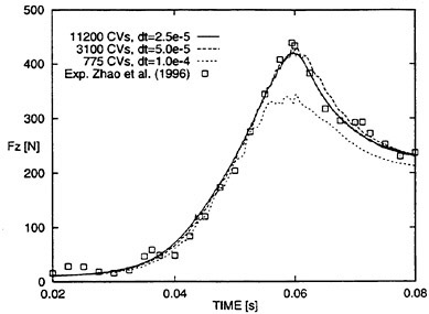
Figure 7: Time series of vertical force on ship section. First set of computations to show effects of systematically refining space and time.
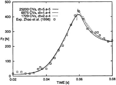
Figure 8: Time series of vertical force on ship section. Second set of computations to find an optimum grid density.
Here nt denotes the number of time steps.
Table 2: CPU times for water entry simulation of the flared ship section.
|
CVs |
nt |
CPU time [h] |
|
11200 |
8300 |
17.01 |
|
3100 |
4150 |
1.84 |
|
775 |
2000 |
0.23 |
|
25200 |
4150 |
33.91 |
|
6975 |
2080 |
3.06 |
|
1729 |
1040 |
0.34 |
3.1.2 Effect of domain size
We investigated the effect of domain size by extending the boundaries of the computational domain. Our intention was to find the minimum domain size that yields domain independent results. In addition the size of the experimental domain (tank) was unknown and we wanted to find out how important this parameter is for results.
All simulations were performed with the 3100 CVs grid and with a time step of Δt=2 · 10−4 s. Table 3 lists the sizes of the domain. Here Ymax is the width of the domain, Zmin is the distance from keel to lower boundary of the domain, and fb is the ratio of Ymax to the half breadth of the ship section (B/2=0.16 m).
Figure 9 shows predicted time series of vertical force together with measurements. Only the two solutions based on the large domains compare favorably with measurements. Locating the horizontal boundary too close (Ymax=0.64 m) to the body overpredicted vertical force. For domains with Ymax=1.6 m and Ymax=2.56 m the difference in predicted forces was negligibly small. Therefore, we performed the subsequent computations with domain size of Ymax=1.6 m and Zmin=−0.717 m to ensure domain size independent results.
Table 3: Particulars of simulations for systematic change of domain size.
|
Ymax [m] |
Ζmin [m] |
fb=Ymax/(B/2) |
|
2.56 |
−1.195 |
16 |
|
1.60 |
−0.717 |
10 |
|
0.64 |
−0.239 |
4 |
3.1.3 Effect of time step size
We investigated the effect of changing the time step size with the 3100 CVs grid. Figure 10 shows the generally favorable agreement of predicted time series of vertical force with measurements. Predicted maximum force at t=0.06 s decreased with decreasing time step size. However, this effect was small.
3.1.4 Local pressure prediction
Predicted vertical forces compared favorably with experimental data. We also examined local pressures along the section girth at three instants of t=0.06 s, t=0.07 s and t=0.08 s. Solutions were obtained with the 3100 CVs grid and 11200 CVs grid (Table 1). Figure 11 shows predicted pressure coefficients
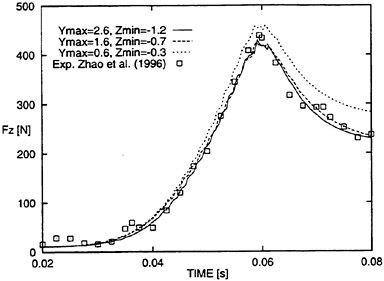
Figure 9: Time series of vertical force on ship section to show effects of systematically changing domain size.
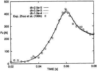
Figure 10: Time series of vertical force on ship section to show effects of systematically refining time step size.
![]() together with experimental data. Pressure measurements were available at four non-dimensional depths ζ=z/D, where z is the local vertical coordinate and D the vertical coordinate of the knuckle of the flared section. A non-dimensional depth of ζ=0 corresponded to the keel. The instantaneous entry velocity is denoted by Ventry(t), and pa is atmospheric pressure.
together with experimental data. Pressure measurements were available at four non-dimensional depths ζ=z/D, where z is the local vertical coordinate and D the vertical coordinate of the knuckle of the flared section. A non-dimensional depth of ζ=0 corresponded to the keel. The instantaneous entry velocity is denoted by Ventry(t), and pa is atmospheric pressure.
Predicted pressure coefficients CP agreed favorably with experimental data at ζ=0.02 and at ζ=0.94 for all three time instants. Differences between the solutions were small at t=0.07s and t=0.08 s for both grids. Differences between solutions were larger at t=0.06 s. At ζ=0.58 and ζ=0.74, CP was overpredicted.
Pressure changes rapidly during water entry, and a small shift in the associated time measurement can significantly effect the corresponding pressure measurements. To illustrate this, Fig. 12 shows the time series of CP at ζ=0.58 and at ζ=0.74 for the fine grid solution shown in Fig. 11. Figure 12 also shows that for t=0.06 s, CP is larger at ζ=0.74 than at ζ=0.58, whereas for t=0.08 s, CP is larger at ζ=0.58 than at ζ=0.74. Our numerical method also predicted this trend.
Disagreement of predicted pressure with pressure measurements (Fig. 12, at t=0.06 s) are inconsistent with the favorable agreement of predicted force with force measurement (Fig. 7, for 11200 CVs and 3100 CVs grid). Zhao et al. (15) mentioned that this inconsistency may be attributed to measurement errors. Schumann’s computations of this flared section also showed an overprediction of pressure coefficients around mid girth (12).
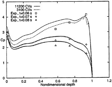
Figure 11: Pressure coefficients CP along section girth for three time instants during water entry.
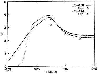
Figure 12: Time series of pressure coefficients CP at two non-dimensional depths ζ=0.58 and ζ=0.74.
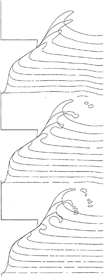
Figure 13: Free surface deformation at consecutive time instants for the grid with 1729 CVs (top), 6975 CVs (middle) and 25200 CVs (Start at t=0.0076 s, time increments of Δt=0.01 s.)
3.1.5 Free-surface deformation
Time series of predicted free surface contours during water entry are shown in Fig. 13. Results were obtained with grids used for the second set of computations (Table 1). Contours are shown at times t=0.01 s apart. After the initial impact of the ship section, the free surface remained attached to the ship section. At the knuckle the free surface separated, producing a splash. Free-surface contours of the splash were different for the three grids. Formation of droplets occurred only with the medium and fine grids. However, solutions based on all grids correctly predicted the general feature of flow separation at the knuckle.
3.2 Water entry of a wedge
3.2.1 Two-dimensional simulations
We employed three two-dimensional grids to investigate effects of grid and time step refinement. Table 4 summarizes particulars of the three grids. Figure 14 shows a partial view of the medium grid. Grid topology and boundary conditions were similar to those of the ship section. We selected a domain size based on the findings of section 3.1.2 to ensure domain size independent results.
Table 4: Particulars for systematic refinement of space and time.
|
CVs |
ny · nz |
Δt [s] |
Δn [m] |
|
17408 |
64 · 64 |
2.5 · 10−5 |
1 · 10−3 |
|
4352 |
32 · 32 |
5.0 · 10−5 |
2 · 10−3 |
|
1280 |
16 · 16 |
1.0 · 10−4 |
4 · 10−3 |
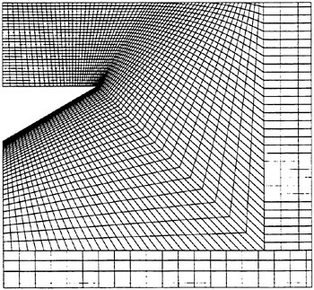
Figure 14: Partial view of computational grid with 4352 CVs.
Figure 15 shows the two-dimensionally computed vertical force Fz on the wedge section for three successively refined grids, including measurement data.
Differences in predicted vertical forces were small. At t=0.016 s the maximum predicted force was smaller for the coarse grid than for the medium and fine grids. Until t=0.01 s, predicted vertical forces agreed closely with measurements. After that time, the forces were overpredicted. Zhao et al. (11) also observed this effect. They attributed this to three-dimensional effects, and they were able to successfully correct their two-dimensional potential flow based solution to account for three-dimensional effects.
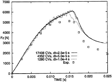
Figure 15: Time series of vertical force on wedge section to show effects of systematically refining space and time.
Table 5 lists the CPU times for the two-dimensional computations described above.
Table 5: CPU times for two-dimensional water entry simulation of the wedge.
|
CVs |
nt |
CPU time [h] |
|
17408 |
3000 |
15.15 |
|
4352 |
1500 |
1.56 |
|
1280 |
750 |
0.21 |
3.2.2 Three-dimensional results
We studied effects of three-dimensional water entry by extending the two-dimensional grid in the longitudinal direction of the wedge. We did not know the spacing Δx in the experiments between the vertical face of the wedge and the tank wall. We were aware that this spacing can significantly influence results because of the strong domain size dependence of results (Fig. 9).
Table 6 lists particulars of the numerical simulations performed to investigate effects of spacing Δx. We gridded this spacing with NX cells in the longitudinal direction. Parameter fl is the ratio of the sum of spacing Δx and half length of the wedge (L/2=0.5 m) to L/2. (For the ship section, a factor fb=10 was necessary to obtain domain size independent results.) We specified a time step of Δt=1 · 10−4 s and a minimum cell width at the girth of the wedge of Δn=2 · 10−3 m. We assumed double symmetry and, therefore, discretized only one quarter of the wedge. The half length of the wedge (L/2) was gridded with nx=16 CVs. The inner block of this coarse three-dimensional grid contained nx · ny · nz=163=4096 CVs. Figure 16 shows a perspective view of this grid. The capability of the numerical method to accommodate non-matching block interfaces significantly eased the three-dimensional grid generation.
Table 6: Particulars of simulations for systematic change of domain size.
|
CVs |
NX |
Δx [m] |
fl=(Δx+L/2)/(L/2) |
|
21760 |
4 |
0.025 |
1.05 |
|
24832 |
8 |
0.100 |
1.20 |
|
34816 |
16 |
0.250 |
1.50 |
|
47104 |
32 |
1.500 |
4.00 |
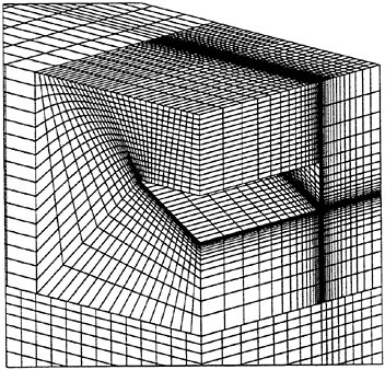
Figure 16: Partial view of computational grid with 34816 CVs (Δx=0.25 m).
Figure 17 shows time series of predicted vertical forces on the wedge for different spacings Δx, including measurement data. The effect of spacing Δx on vertical force became noticeable at t=0.08 s. As expected, a smaller spacing increased the predicted
vertical force. A spacing of Δx=0.25 m appeared to match the experimental data most favorably.
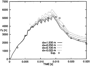
Figure 17: Time series of vertical force on wedge section to show effect of changing spacing Δx between the wedge and the lateral boundary.
Therefore, to investigate effects of systematic refinement in space and time for the three-dimensional case with spacing Δx=0.25 m, we generated a medium three-dimensional grid comprising 206848 CVs, of which nx·ny·nz=323=32768 CVs were assigned to the inner block. For this grid we selected a time step of Δt=5·10−5 s and a minimum cell width of Δn=1 · 10−3 m. Figure 18 shows the predicted forces for the coarse and medium three-dimensional grids and a reference two-dimensional result together with experimental data. The solution obtained with the medium grid exhibited an expected behavior, i.e., maximum predicted force increased until t=0.016 s and then decreased with a greater gradient than the solution based on the coarse grid. Two-dimensional results showed the same effect (Fig. 15). Judging from the predicted vertical force obtained with the medium three-dimensional grid, it appeared that the spacing Δx between the wedge and the tank wall was smaller than 0.25 m.
Table 7 lists the CPU times for three-dimensional computations described above. To save CPU time, we performed the simulation on the 206848 CVs grid until water entry of the keel with fewer time steps.
Table 7: CPU times for three-dimensional water entry simulation of the wedge.
|
CVs |
nt |
CPU time [h] |
|
206848 |
780 |
88.92 |
|
34816 |
750 |
9.25 |
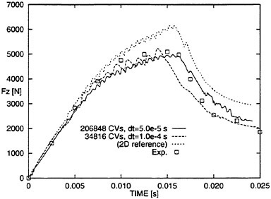
Figure 18: Time series of vertical force on wedge section to show effects of systematically refining space and time for the three-dimensional case.
3.2.3 Local pressure prediction
Figure 19 shows predicted pressure coefficients CP along the girth obtained with the three successively refined grids (Table 4). We selected three time instants corresponding to t=0.00435 s, t=0.0158 s, and t=0.0202 s. At t=0.00435 s only part of the girth was wetted, and local pressure increased from keel to the spray root. The numerical method did not predict maximum CP at this instant of time. At a small instant of time later, however, we suspect that predicted pressures would have been greater, thereby comparing more favorably with measurements. At t=0.0158 s, CP was overpredicted for all non-dimensional depths except for ζ=0.91. At t=0.0202 s, CP was overpredicted for all nondimensional depths. Zhao et al. (11) also observed this behavior, and they stated that this was due to three-dimensional effects in the experiment.
Figure 20 shows predicted local pressures for the three-dimensional case based on the 206848 CVs grid. Two-dimensional results and measurements are included for comparison. In general, the three-dimensionally predicted pressures were lower than those obtained with a two-dimensional grid and tended to compare more favorably with measurements. Apparently, the 206848 CVs grid was not sufficiently fine to capture the maximum pressures recorded in the experiments.
3.2.4 Free-surface deformation
Figure 21 shows time series of two-dimensionally predicted free-surface contours obtained with the 17408 CVs grid. Contours are shown at times incremented by t=0.0025s s. The free surface remained attached
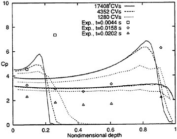
Figure 19: Pressure coefficients CP along girth for three time instants during water entry to show effects of grid refinement.
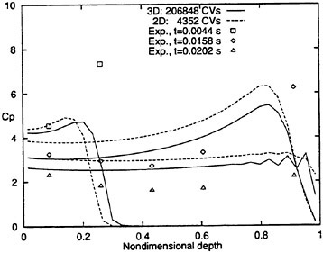
Figure 20: Pressure coefficients CP along girth for three time instants during water entry to show three-dimensional effects.
to the wedge until separating at the knuckle, forming a splash. At the last time instant shown, part of the splash detached.
Figure 22 (see the last page) shows two perspective views of three-dimensionally predicted free-surface deformations at two time instants during water entry of the wedge. Graphs a) and b) refer to the time instant t=0.0136 s when the free surface was still fully attached to the wedge. Only small three-dimensional effects influenced the flow pattern in the longitudinal direction of the wedge. Graphs c) and d) refer to the time instant t=0.0236 s when the top of the wedge was close to the still water level. Significant three-dimensional free-surface deformations occurred in the vicinity of the vertical face of the wedge, specially near the upper corner. At the vertical face of the wedge a steep splash developed, leading to a
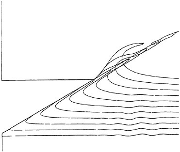
Figure 21: Free-surface deformation at consecutive time instants for the 17408 CVs grid. (Start at t=−0.00125 s, time increments of Δt=0.0025 s.)
nearly vertical free-surface deformation that caused the vertical face of the wedge to remain dry during the entire simulation.
4 Conclusions
The presented method modeled two phenomena relevant for water entry problems, namely, viscous effects and the nonlinear nature of the free-surface deformation. The free-surface capturing model predicted the development of the free surface, including breaking and overturning of waves. The finite volume discretization technique dealt with complex geometries based on control volumes with an arbitrary number of cell faces.
Our method was systematically applied to simulate two problems of water entry. Numerical results were compared with measurements of (11). We investigated effects of refining space and time, effect of changing domain size, as well as importance of initial conditions and boundary conditions. Results showed that the discretization errors were relatively small and that favorable agreements with experimental data was achieved even with relatively coarse grids. Numerical experiments indicated that the size of the experimental domain (tank) and the motion history of the entering body influenced pressures and forces exerted on the body. Accurate measurements as well as detailed description of experimental setups are therefore essential to validate numerical methods.
The method proved to be sufficiently robust and reliable and can be applied, for example, to predict
impact pressures in the design stage of a ship.
Acknowledgments
This work was partially supported by the Ministry of Education, Science, Research and Technology of the Federal Republic of Germany under contract MTK 0577A. The opinions expressed herein are those of the authors.
References
1. Farmer, J., Martinelli, L., Jameson, A., “Fast multigrid method for solving incompressible hydrodynamic problems with free surface”, AIAA J., Vol. 32, 1994, pp. 1175–1182.
2. Muzaferija, S. and Perić, M., “Computation of free-surface flows using finite volume method and moving grids”, Numer. Heat Transfer, Part B, Vol. 32, 1997, pp. 369–384.
3. Hirt, C.W., and Nichols, B.D., “Volume of fluid (VOF) method for dynamics of free boundaries”, J. Comput. Phys., Vol. 39, 1981, pp. 201–221 ().
4. Harlow, F.H., and Welsh, J.E., “Numerical calculation of time dependent viscous incompressible flow with free surface”, Phys. Fluids, Vol. 8, 1965, pp. 2182–2189.
5. Kawamura, T., and Miyata, H., “Simulation of nonlinear ship flows by density-function method”, J. Soc. Naval Architects Japan, Vol. 176, 1994, pp. 1–10.
6. Lafaurie, B., Nardone, C., Scardovelli, R., Zaleski, S., and Zanetti, G., “Modeling merging and fragmentation in multiphase flows with SURFER”, J. Comput. Phys., Vol. 113, 1994, pp. 134–147.
7. Ubbink, O., Numerical prediction of two fluid systems with sharp interfaces, PhD thesis, University of London, 1997.
8. Muzaferija, S., and Perić, M., “Computation of free surface flows using interface-tracking and interface-capturing methods”, chap. 3 in O.Mahrenholtz and M.Markiewicz (eds.), Nonlinear Water Wave Interaction, Computational Mechanics Publications, Southampton, 1998.
9. Arai, M., Cheng, L.-Y., and Inoue, Y., “A Computing Method for the Analysis of Water Impact of Arbitrary Shaped Bodies”, J. Society of Naval Architects of Japan, Vol. 176, 1994, p 233.
10. Troesch, A.W., Kang, C.-G., “Evaluation of Impact Loads Associated with Flare Slamming”, J. Society of Naval Architects of Korea, Vol. 27, No. 3, 1990, p 56.
11. Zhao, R., Faltinsen, O.M., and Aarsens, J., “Water entry of arbitrary two-dimensional sections with and without flow separation”, Proceedings of the Twenty-First Symposium on Naval Hydrodynamics, Trondheim, June 24–28, 1996.
12. Schumann, C., “Volume-of-fluid Computations of Water Entry of Bow Sections”, Proceedings of EUROMECH 374, Poitiers, April 1998.
13. Sames, P.C., Schellin, T.E, Muzaferija, S., and Perić, M., “Application of a Two-Fluid Finite Volume Method to Ship Slamming”, for presentation at 17th Int. Con. Offshore Mechanics and Arctic Engineering (OMAE), Lisbon, July 1998.
14. Demirdžić, I., Muzaferija, S., and Perić, M., “Advances in computation of heat transfer, fluid flow, and solid body deformation using finite volume approach”, in W.J.Minkowycz, E.M.Sparrow (eds.), Advances in Numerical Heat Transfer, chap. 2, pp. 59–96, Taylor and Francis, New York, 1996.
15. Leonard, B.P, “Bounded higher-order upwind multidimensional finite-volume convection-diffusion algorithms”, in W.J.Minkowycz, E.M.Sparrow (eds.), Advances in Numerical Heat Transfer, chap. 1, pp. 1–57, Taylor and Francis, New York, 1996.

Figure 22: Free surface deformation at two time instants for the 206848 CVs grid. Graphs a) and b) at t=0.0136 s, graphs c) and d) at t=0.0236 s.
DISCUSSION
U.Bulgarelli
Istituto Nazionale per Studi ed Esperienze di Architettura Navale, Italy
Is it easy to extend the method in 3D cases? Because in this case you have a more complex topology of cell and also a 3D theory of characteristic of hyperbolic part of the equations?
AUTHORS’ REPLY
The method has a 3D implementation and the results presented in the paper are also three-dimensional. The authors did not have any problems in calculating a development of the free-surface for three-dimensional cases using the method presented.
DISCUSSION
T.Hino
Ship Research Institute, Japan
According to the Courant number correction (10), the spatial discretization scheme selected is dependent on the time step used. It means that, when the method is applied to steady-state problems, the final solution is dependent on the time step size. Is it necessary to limit a time step size in order to avoid too much diffusion of interface?
AUTHORS’ REPLY
The Courant number correction in the HRIC scheme is based on the velocity component normal to the interface. In order to keep interface sharp, it is necessary to use a relatively small time step, such that interface does not cross more than a half a cell during one time step. As the steady state is approached, the interface moves slower and slower (i.e. the velocity component normal to the interface tends to zero), so the Courant-number correction stops playing an important role.
Water Entry of Arbitrary Axisymmetric Bodies With and Without Flow Separation
R.Zhao (Marintek, Norway)
O.Faltinsen (Norwegian University of Science and Technology, Norway)
1 ABSTRACT
Two different theoretical methods for predicting slamming loads on axisymmetric bodies have been developed. One of the methods is a fully nonlinear numerical simulation and the other method is an extension of two-dimensional Wagner’s solution (1932). Both methods include the effect of flow separation from knuckles or fixed separation points of a body with continuously curved surface. The numerical results have been compared with an asymptotic solution and experimental data.
2 INTRODUCTION
Impact or slamming loads are important for the design of ships and offshore structures. Since the pioneering works by von Karman (1929) and Wagner (1932), many experimental, analytical and numerical studies have been reported. We will focus on the slamming loads on axisymmetric bodies with and without flow separation from knuckles. This is a first step towards developing a rational method for three-dimensional slamming load on ships.
Water entry of axisymmetric bodies with small local deadrise angles are studied analytically by for instance Shiffman and Spencer (1951), Chuang (1969) and Faltinsen and Zhao (1997). The methods are based on generalizations of Wagner’s (1932) theory for water entry of a two-dimensional body. The outer flow solutions are studied by Shiffman and Spencer (1951) and Chuang (1969). Faltinsen and Zhao (1997) used the outer flow solution to match a inner jet flow solution and a composite solution for the pressure distribution on the body was constructed.
In order to study the slamming load on an arbitrary axisymmetric body with flow separation from knuckles, two different numerical methods are developed. One of the methods represents a fully nonlinear solution, which is a further development of the work by Zhao and Faltinsen (1993) and Zhao et al. (1996). They studied slamming loads on two-dimensional sections with and without the effect of flow separation. The problem was solved as an initial value problem. The fully nonlinear free-surface conditions without gravity and exact body boundary condition were used in the numerical analysis. A local jet flow was introduced near the intersection between the body surface and the free surface. The method was verified by Zhao and Faltinsen (1993) by comparing with analytical and asymptotic solutions for symmetrical wedges with deadrise angles from 4° to 81°. The method was validated by experimental drop tests of Zhao et al. (1996) for a bow flow section and a wedge with knuckles. We will now extent the numerical method of Zhao and Faltinsen (1993) and Zhao et al. (1996) to general axisymmetric bodies with arbitrary vertical velocity. The flow separation from knuckles and bodies with convex shape is included in the numerical analysis. The separation point is assumed fixed. When the separation occurs for a continuously curved surface, the separation point will be determined empirically. Comparisons are made with an asymptotic solution valid for small local deadrise angles and without flow separation. Further the method is validated by comparing with published experimental data.
An approximate solution of axisymmetric bodies based on a generalization of Wagner’s solution (1932) was presented by Faltinsen and Zhao (1997). The flow separation was not included in the analysis. The body boundary condition was satisfied exactly. The piled-up water around the intersection between the free surface and the body surface was calculated using a similar approach as Wagner (1932) did in two-dimensional flow. The velocity potential was set equal to zero on a horizontal plane outside the body and going through the intersection line between the free surface and the body surface. The pressure distribution on the body surface was obtained as a function of time. This method is now generalized to include the effect of flow separation. The approximate solution has been checked with the analytical and the fully nonlinear numerical solution. Satisfactory agreement of the maximum pressure
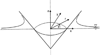
Figure 1: Water entry of an axisymmetric body. Definition of a Cartesian coordinate system (x,y,z) and a polar coordinate system rθz.
and total slamming loads are obtained. This approximate solution is fast to calculate and useful in practical applications.
3 FULLY NONLINEAR SOLUTION
A general axisymmetric body with time dependent vertical downwards velocity, is forced through initially calm water. The problem is solved as an initial value problem. Since viscous effects are neglected, the problem can be solved by potential theory. The effects of compressibility of the water and air cushions between the water and the structure are neglected. Gravity is not included in the analysis. This has a negligible effect in the initial phase of water entry of a blunt body, but will be more important at a later stage after flow separation has occurred.
The reference coordinate systems xyz and rθz are fixed in space. The xyz is a Cartesian coordinate system and rθz is a polar coordinate system. The origin of the coordinate systems are in the plane of the undisturbed water surface. The z-axis is positive upwards (see figure 1). The velocity potential ![]() satisfies the Laplace equation
satisfies the Laplace equation
(1)
in the fluid domain. The dynamic free-surface condition on the exact free surface can be written as
(2)
D/Dt means the substantial derivative and t is the time variable. The kinematic free-surface condition is that a fluid particle remains on the free surface. Hence the free surface can be found by convecting particles on the free surface with the local fluid velocity. The body boundary condition on the wetted body surface is satisfied on the instantaneous body surface. It can be written as
(3)
where Vn is the body velocity in the normal direction ![]() on the body surface. Positive direction of
on the body surface. Positive direction of ![]() is into the fluid domain. The initial conditions are zero velocity potential and free-surface elevation.
is into the fluid domain. The initial conditions are zero velocity potential and free-surface elevation.
The problem with and without flow separation will be solved similarily as the two-dimensional solution by Zhao and Faltinsen (1993) and Zhao et al. (1996). A jet flow is created at the intersection between the free surface and the body surface. The thin jet will not contribute much to the total force on the body (see Zhao et al. (1996)). The part of the jet, where the pressure is close to atmospheric pressure, can therefore be neglected. This makes it unnecessary to find the intersection line between the body and free surface. The intersection angle is very small for bodies with small deadrise angles and will cause numerical problems (Greenhow (1987)). The geometry of the body may be either convex or concave around the spray root of the jet flow (see figure 2). One should cut the jet before it leaves the body in the numerical simulations (see figure 2). The thin jet will follow the body surface for a body with concave shape (see figure 2), but it will give a small force on the body surface. Therefore one may cut the most part of the jet.
An instantaneous fluid domain Ω that does not contain the whole jet flow, is defined. The jet flow is cut at AB (see figure 2). The velocity potential ![]() for the flow inside the fluid domain is represented by Green’s second identity, i.e.
for the flow inside the fluid domain is represented by Green’s second identity, i.e.
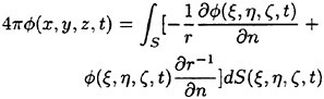
(4)
where ![]() means derivative in the normal direction of S. Positive direction is into the fluid domain. The surface S consists of AB, SB,
means derivative in the normal direction of S. Positive direction is into the fluid domain. The surface S consists of AB, SB,
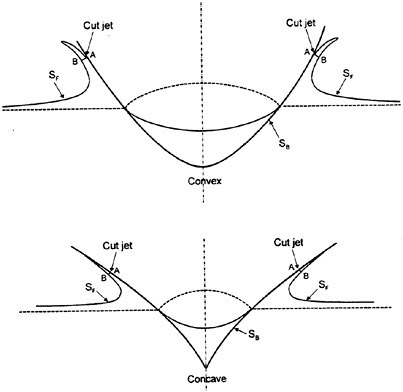
Figure 2: The water entry of axisymmetric bodies with convex and concave shapes. The jet is cut at AB in the numerical simulations. SF is the free surface.
SF and SC. Here SB is the instantaneous wetted body surface below A, SF is the instantaneous free surface, SC is a control surface infinitely faraway from the body. The contribution from integrating over SC in equation (4) is zero. The contribution from the free surface far away from the body can be rewritten. The velocity potential ![]() b(t), where b(t) is large relative to the cross-dimensions of the hull, can be expressed as a vertical dipole in infinite fluid. The reasons are that the flow is axisymmetric about z-axis and the free surface condition is
b(t), where b(t) is large relative to the cross-dimensions of the hull, can be expressed as a vertical dipole in infinite fluid. The reasons are that the flow is axisymmetric about z-axis and the free surface condition is ![]() from a far-field point of view,
from a far-field point of view, ![]() can then be written as
can then be written as
(5)
where C1(t) is an unknown that is found as a part of the solution.
An integral equation based on equation (4) is set up by letting (r,z) approach points on S for each time step. Since the flow and the body geometry are axisymmetric about the z-axis, the free surface SF inside |r|=b(t), and the body surface SB, are divided into a number of ring segments in the numerical evaluation of this integral equation, ![]() and
and ![]() are set constant on each element, except on AB, where
are set constant on each element, except on AB, where ![]() has a linear variation over the element. For each
has a linear variation over the element. For each

Figure 3: The water entry of an axisymmetric body with flow separation at the knuckle. When the spray root of the jet reaches the separation point S, a part of the jet is introduced in the numerical simulation.
element on the free surface inside |r|=b(t), and on AB ![]() is known and
is known and ![]() is unknown. The instantaneous position of these elements and the values of
is unknown. The instantaneous position of these elements and the values of ![]() follow from the free-surface conditions. Special care is needed in describing the motion of the free surface in order to satisfy conservation of fluid mass. A second order description of the free surface is used in areas with large curvature. On the body surface
follow from the free-surface conditions. Special care is needed in describing the motion of the free surface in order to satisfy conservation of fluid mass. A second order description of the free surface is used in areas with large curvature. On the body surface ![]() is unknown and
is unknown and ![]() is known. In addition there is one unknown which comes from the representation of the far field solution. The total number of unknowns is NB+NF+1, where ΝΒ is number of elements on the body surface and ΝF is number of elements on the free surface and on AB. The integral equation resulting from equation (4) is satisfied at the midpoint of each element on SB, SF, AB and at one control point in the fluid domain with |r|-value larger than b(t). One obtains then a system of linear equations with the same number of equations as number of unknowns. The linear equations are solved by a standard procedure. AB (see figure 2) is not used in the initial phase. When the free surface at the intersection with the body is close to the slope of the body surface, AB is introduced.
is known. In addition there is one unknown which comes from the representation of the far field solution. The total number of unknowns is NB+NF+1, where ΝΒ is number of elements on the body surface and ΝF is number of elements on the free surface and on AB. The integral equation resulting from equation (4) is satisfied at the midpoint of each element on SB, SF, AB and at one control point in the fluid domain with |r|-value larger than b(t). One obtains then a system of linear equations with the same number of equations as number of unknowns. The linear equations are solved by a standard procedure. AB (see figure 2) is not used in the initial phase. When the free surface at the intersection with the body is close to the slope of the body surface, AB is introduced.
It will now be described how to solve the problem when the flow separates from a knuckle (or a fixed separation point). When AB reaches the separation point S, a part of the previously neglected jet is introduced. The computational domain will then include a larger part of the jet (see figure 3). The reason for doing this is to avoid numerical difficulties. The thin jet, which has been introduced here, is assumed to have the same thickness and constant velocities in the r and z-direction for the whole jet. The length of the introduced jet part is about 6 times the length of AB. In reality the thickness will not be the same. For instance the angle at the intersection between the water and

Figure 4: The local two-dimensional polar coordinate system (r1, θ1) and the local two-dimensional Cartesian coordinate system (s1, n1) are shown. S is the separation point, SB the body surface and SF the free surface. The s1-coordinate coincides with the tangent of the body surface at the separation point S.
the body surface is about 1.8° during water entry with constant velocity of a wedge (2-D) with deadrise angle 30°. It is assumed that the angle is also small for an axisymmetric body. The length of the total jet is the same order as the length of the wetted body surface when the wetted surface is defined as the distance from the keel to the spray root of the jet. The introduced jet part is therefore a small portion of the whole jet. It is a good approximation to assume constant jet thickness in this part of the jet. The numerical results are not sensitive to the length of the introduced jet part. A hemicircle is used at the end of the jet. This is advantageous in the time stepping of the solution.
A Kutta condition is applied at the separation point S. This implies that the flow leaves tangentially at the knuckle and the velocity at point S is finite. In a small region near the knuckle the behaviour of the velocity can be studied by a local two-dimensional analysis.
Here a local two-dimensional polar coordinate system (r1θ1) and a local two-dimensional Cartesian coordinate system (s1, n1) are used (see figure 4). A local solution of the velocity potential ![]() that satisfies the body boundary condition, can be written as
that satisfies the body boundary condition, can be written as
(6)
The velocity potential ![]() satisfies the free-surface condition
satisfies the free-surface condition
(7)
This leads to the following approximation for small r1
(8)
The lowest order term in equation (8) is
(9)
This equation says simply that the pressure is atmospheric pressure at the separation point. This is automatically satisfied as a part of the solution. The next term in equation (8) gives
(10)
Possible values of n are ![]() cannot be a solution since it leads to a singular velocity. Choosing
cannot be a solution since it leads to a singular velocity. Choosing ![]() is consistent with that
is consistent with that ![]() should be a smaller term then
should be a smaller term then ![]() . This means that the solution in the vicinity of the separation point can be written as
. This means that the solution in the vicinity of the separation point can be written as
(11)
Equation (11) implies that the tangential velocity at the free surface is U(t). Close to the separation point, the tangential velocity at the body surface can be written as
(12)
The free surface near the separation point can be found by equation (11). It can be shown that the flow leaves the knuckle tangentially. Very small elements are used near the knuckle in the numerical calculations. The length of the segments used near the knuckle on the body and free surface is about 0.3% of the length of the wetted body surface for the cone with deadrise angle 30°. Therefore the tangential velocity for the segments closest to the knuckle on the body can be approximated by the particle velocity on the free surface closest to the knuckle. This means that the last term in equation (12) is neglected. The numerical details of the implementation of the conditions at a separation point are described below.
Figure 5 shows the element distribution around a knuckle. Based on the velocity potentials at points A, B and D, the tangential velocity at point Β can be estimated. Based on
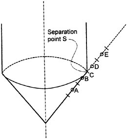
Figure 5: Element distribution and midpoints A, B, D and E of the elements near the separation point S.
the velocity potentials at points B, D and E the tangential velocity at point D can be estimated. These two velocities are set equal. This gives a linear relationship between unknown velocity potential values on the body surface and known potential values of the free surface near the separation point. In addition the normal derivative ![]() of the potential near the knuckle is set equal on the body and the free surface. These two relationships implies that two equations in the linear equation system that follows from the integral equation based on equation (4) must be excluded. This is done by not satisfying the integral equation at the closest segments to the knuckle on the body and free surface.
of the potential near the knuckle is set equal on the body and the free surface. These two relationships implies that two equations in the linear equation system that follows from the integral equation based on equation (4) must be excluded. This is done by not satisfying the integral equation at the closest segments to the knuckle on the body and free surface.
When the solution is stepped from time ti to ti+1, the free surface location and velocity potential on the free surface for ti+1 are obtained by using the kinematic and the dynamic free-surface conditions. Because the velocities on the body and free surface for the elements closest the separation point are the same, the element closest to the separation point on the free surface will always be located on the tangential continuation of the body surface from the separation point.
The front part of the jet has larger velocities than the rest of the fluid in the beginning of flow separation from the knuckle. Number of elements to represent the jet must therefore be increased as time goes. It is also found that the free surface can be unstable at the front part of the jet. This problem can be suppressed for a long time by cutting the front part of the jet. It has been checked that this does not affect the pressure on the body surface. The particle velocities near the original jet flow will be strongly reduced at a late stage. This means that it is not really a jet flow anymore. It should also be noted that the acceleration of fluid particles will not be much larger than the gravitational acceleration at a late stage of the flow. The effect of gravity should therefore be included in the numerical simulation at this stage. This has not yet been studied.
The pressure p on the body surface is calculated by Bernoulli’s equation, which can be written as
(13)
Here the hydrostatic pressure is neglected. pa is atmospheric pressure and ρ is the mass density of the fluid. The term ![]() is found by generalizing the concept of substantial derivative. One introduces
is found by generalizing the concept of substantial derivative. One introduces
(14)
where ![]() is the change in
is the change in ![]() when one follows the mid-point of a segment, that moves with velocity
when one follows the mid-point of a segment, that moves with velocity ![]() .
.
4 SIMPLIFIED SOLUTION
Wagner (1932) developed an asymptotic solution for water entry of two-dimensional bodies with small local deadrise angles. The flow was studied in two fluid domains. The inner flow domain contains a jet flow at the intersection between the body and the free surface. In the outer flow domain the body boundary condition and the dynamic free-surface condition ![]() were transformed to a horizontal line. The kinematic free-surface condition was used to determine the intersection between the free surface and the body in the outer flow domain. Zhao and Faltinsen (1993) presented a composite solution for the pressure distribution in the outer and inner flow domain and showed satisfactory agreement with similarity solutions for wedges with deadrise angles smaller than 20°.
were transformed to a horizontal line. The kinematic free-surface condition was used to determine the intersection between the free surface and the body in the outer flow domain. Zhao and Faltinsen (1993) presented a composite solution for the pressure distribution in the outer and inner flow domain and showed satisfactory agreement with similarity solutions for wedges with deadrise angles smaller than 20°.
A generalization of Wagner’s solution to larger local deadrise angles was presented by Zhao et al. (1996). A main difference from Wagner’s (1932) theory was that the exact body boundary condition was satisfied at each time instant. The wetted body surface was found by integrating in time the vertical velocities of fluid particles on the free surface and finding when the particles intersected the body surface. Wagner did also that, but he could use analytical solutions because of the simplified body boundary condition. The dynamic free-surface condition will be the same as Wagner used. The pressure is calculated by the complete Bernoulli’s equation (equation (13)) without gravity. It has not been possible to find an inner flow solution near the spray roots that matches the outer flow solution. This would have made it possible to exclude in a rational way the large negative pressures that occur at the intersection points in our outer flow solution. The procedure
was simply to neglect the negative pressures. The method was modified by Faltinsen and Zhao (1997) to axisymmetric bodies. We are now to generalize the method for water entry of an axisymmetric body with flow separation from the knuckle or a fixed point.
The problem is solved as an initial value problem. The velocity potential satisfies three-dimensional Laplace equation in the fluid domain. A boundary value problem is solved by using equation (4) for each time step. The numerical procedure is similar as the fully nonlinear problem. A coordinate system r1 z1 which follows the vertical motion of the body is used (see figure 6). The dynamic free surface condition ![]() is satisfied on horizontal plane that starts at the intersection line between the body and the free surface see (figure 6). The dynamic free surface condition implies that fluid particles on the free surface have only vertical velocities.
is satisfied on horizontal plane that starts at the intersection line between the body and the free surface see (figure 6). The dynamic free surface condition implies that fluid particles on the free surface have only vertical velocities.
The numerical simulation starts at time t0. The submergence of the body is ![]() at t0 (see figure 6). The effect of free-surface elevation is neglected initially, so the free surface l0 is horizontal. In the numerical computation, t0 is set equal to 0.15tpout, where tpout is the time instance when one needs the pressure distribution and slamming forces as output. This procedure has been tested against the Wagner solution for a water entry of a circle (2-D) at an early stage and water entry of a wedge (2-D) with small deadrise angles. Satisfactory predictions of the pressure distribution and the slamming forces were obtained.
at t0 (see figure 6). The effect of free-surface elevation is neglected initially, so the free surface l0 is horizontal. In the numerical computation, t0 is set equal to 0.15tpout, where tpout is the time instance when one needs the pressure distribution and slamming forces as output. This procedure has been tested against the Wagner solution for a water entry of a circle (2-D) at an early stage and water entry of a wedge (2-D) with small deadrise angles. Satisfactory predictions of the pressure distribution and the slamming forces were obtained.
After the velocity potential on the body surface has been determined, the pressure distribution on the body can be found from equation (13). Special care is shown near the intersection between the body and the free surface. Since the velocity is infinite there, the last term in equation (13) will be negative infinite. It can be shown that the first term is positive infinite at the intersection line, and that the last term is more singular than the first term. Therefore the total pressure is negative infinite. But this is an integrable singularity. Let us define the integrated vertical force for the part with negative pressure as FN, and from the part with positive pressure as FP. It can be shown that FN/FP goes to zero when the deadrise angle goes to zero. For small deadrise angles, the maximum pressure (positive) is obtained near the intersection line. The maximum pressure obtained from the outer solution is the same as the maximum pressure from the composite solution based on Wagner’s solution (Faltinsen and Zhao (1997)) when the deadrise angle goes to zero.
Flow separation from knuckle
A simple analysis of the flow separation problem will be described. The separated free surface from the knuckle
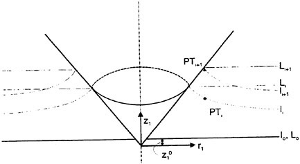
Figure 6: The coordinate system (r1, z1), the real free surface li and li+1 and the horizontal planes Li and Li+1 used in the numerical simulation for time instance ti and ti+1.
is assumed to be a continuation of the body surface with pressure equal to atmospheric pressure. The horizontal line L (see figure 6) is determined in the same way as before as if the separated free surface is a part of the body surface. The problem is how to find the shape of the fictitious “body surface”. Important information can be obtained by studying the shape of the separated free surface near a separation point. Figure 4 shows a local polar coordinate system (r1, θ1) and a local Cartesian coordinate system (s1, n1) at the separation point. Using a Kutta condition at the separation point S implies that the flow leaves tangentially and the velocity at point S is finite. In a small region near the separation point, the behaviour of the velocities can be found by a local analysis. A local solution of the velocity potential ![]() that satisfies the body boundary condition, is given in equation (11). The free surface near the separation point can be found by equation (11) and written as
that satisfies the body boundary condition, is given in equation (11). The free surface near the separation point can be found by equation (11) and written as
(15)
Equation (15) is valid for small s1. However numerical tests have shown that the formula can be used for quite large s1. Further numerical results for the pressure on the “real” body surface are not sensitive to values of C(x). The calculation procedure is an iterative process. A shape of the separated free surface is assumed based on equation (15) and the kinematic free surface condition is satisfied on the assumed free surface. The shape of the separated free surface is iterated until the difference between the pressure on the separated free surface and atmospheric pressure is minimized.
5 VERIFICATION AND VALIDATION
The comparison between the fully nonlinear and simplified solution have been carried out for cones with different deadrise angles and an axisymmetric body with the geometry based on a two-dimensional bow flare section of a ship.
Figure 7 shows the comparison of the numerical results of cones with deadrise angles 10°, 20°, 30°, 45°, 60° and 80°. The fully nonlinear and simplified solution are used to predict the pressure distributions. Good agreement between the two solutions is obtained in particularly for the smaller tested deadrise angles. For deadrise angles 10°, 20° and 30° the asymptotic solution of Faltinsen and Zhao (1997) is also presented. There is a good agreement between the two numerical solutions and the asymptotic solution for the deadrise angles of 10° and 20°.
Figure 8 shows the total slamming force for the cones with different deadrise angles. Both fully nonlinear and simplified theory are presented. The asymptotic solution of Faltinsen and Zhao (1997) is also plotted. For small deadrise angle the fully nonlinear solution and the simplified solution agree well with the asymptotic solution, but not for large deadrise angles. The fully nonlinear solution and the simplified solution agrees quite well for all deadrise angles. The empirical formula based on experimental data of Watanabe (1930) is also plotted. Watanabe (1930) did drop tests of cones for deadrise angle between 5° and 20°. An empirical force formula that depends on the structural mass Μ of the dropped object was presented. The results in figure 8 are obtained by letting Μ goes to infinite. The agreement between the numerical methods and the empirical formula is good except that the empirical formula give a small increase of the non-dimensional value with increasing the deadrise angle. The wetted factor Cw is shown in figure 9. Here Cw is defined as
(16)
where Zw is the vertical distance from the keel to the point where the pressure is equal to atmospheric pressure. For the asymptotic solution Zw is the vertical distance from the keel to the point where the pressure is maximum. There is quite good agreement between the two theories. The ratio of the wetted factor between axisymmetric cones and two-dimensional wedges is shown in figure 10. The wetted surface will be reduced due to three-dimensional effect. The reduction factor is about 0.8. Then the total slamming force will be reduced due to reduction of the wetted surface.
In order to study the three dimensional effect of slamming load on a ship, an axisymmetric body with the geometry based on a two-dimensional bow flare section of a ship is studied. The geometry is shown in figure 11. The total slamming forces are shown in figure 12. The pressure distribution on the body surface before flow separated from the knuckle is shown in figure 13. The pressure distributions are shown for three time instances. The fully nonlinear solution and the simplified solution are compared with each other. Good agreement is obtained.
The effect of flow separation is included in the fully nonlinear and the simplified solution. After the flow separation from the knuckle the slamming force will be reduced. It is interesting to find out how fast the total slamming force drops down. This is for instance important for a planing boat in the steady forward motion and the stability in waves. The numerical results are presented for cones and an axisymmetric body with the geometry based on a two-dimensional bow flare section of a ship. The results are presented in figure 12, 14, 15 and 16. Figures 14 and 15 show the total slamming forces and pressure distribution on a cone with deadrise angle 30°. Figures 12 and 16 show the total slamming forces and pressure distribution on an axisymmetric bow flare section. Both the fully nonlinear and simplified solutions are used. Good agreement between the theories is obtained. Watanabe (1930) and Chuang and Milne (1971) did experiment of cones with knuckles, but no slamming forces after flow separation were presented. Zhao et al. (1996) did experiment with flow separation from a wedge (2-D) with deadrise angle 30° and a bow flare section (2-D). Good agreement between the numerical and experimental results were reported for the slamming loads after flow separation. The two-dimensional bow flare section is used to generalize the asymmetric body.
6 CONCLUSIONS
Two theoretical methods to predict slamming loads on an arbitrary axisymmetric body are presented. One is the fully nonlinear solution without gravity and other is the generalization of Wagner’s solution. Both methods can handle flow separation from knuckles. Numerical results are presented for cones with different deadrise angles and an axisymmetric body with the geometry based on a two-dimensional bow flare section of a ship. Good agreement between the theories is obtained both before and after flow separation. The theories have been also verified and validated by an asymptotic solution and experiments.
7 REFERENCES
Chung, S.L. “Theoretical investigations on slamming of cone-shaped bodies,” J. Ship Res., Vol. 13, No. 4, pp. 276–283, 1969.
Chung, S.L. and Milne, D.T. “Drop test of cones to investigate the three-dimensional effects of slamming,” NSRDC report 3543, 1971.
Greenhow, M. “Wedge entry into initially calm water,” Appl. Ocean Res., Vol. 9, pp. 214–223, 1987.
Faltinsen, O.M. and Zhao, R. “Water entry of ship sections and axisymmetric bodies,” AGARD FDP and Ukraine Institute of Hydromechanics Workshop on “High Speed Body Motion in Water”, 1997.
Shiffman, M. and Spencer, D.C. “The force of impact on a sphere striking a water surface,” AMP rep. 422B, AMG-NYU, No. 133, 1951
von Karman, T., “The impact of seaplane floats during landing,” N.A.C.A. TN321, Washington, 1929.
Wagner, H., “Über stoss- und Gleitvergänge an der Oberflache von Flüssigkeiten,” Zeitschr. f. Angew. Math, und Mech., Vol. 12, No. 4, pp. 193–235, 1932.
Watanabe, S., “Resistance of impact on water surface, Part I-Cone and Part II-Cone (continued),” Institute of Physical and Chemical Research, Tokyo, (Scientific papers), Vol. 12, pp. 251–267, 1929, and Vol. 14, pp. 153–168, 1930.
Zhao, R., Faltinsen, O.M., “Water entry of two-dimensional bodies,” J. Fluid Mech., Vol. 246, pp. 593–612, 1993.
Zhao, R., Faltinsen, O.M., Aarsnes, J.V. “Water entry of arbitrary two-dimensional sections with and without flow separation,” 21st Symposium on Naval Hydrodynamics, 1996.
Zhao, R., Faltinsen, O.M., Haslum, H.A. “A simplified nonlinear analysis of a high-speed planing craft in calm water,” 4th International Conference on Fast Sea Transportation, Australia, 1997.
Figure 7: See caption on p. 660.
Figure 7: Numerical results of pressure distribution p of cones with deadrise angle 10°, 20°, 30°, 45°, 60° and 80°. The fully nonlinear and simplified solutions are used. The asymptotic solution is presented for deadrise angles 10°, 20° and 30°. The vertical axis is (p−pa)/(0.5ρV2). z is the vertical coordinate (defined in figure 1), V the constant vertical velocity, t the time, pa the atomspheric pressure and ρ the mass density of the fluid.
Figure 8: Numerical results of total slamming force F3 of cones with different deadrise angles β. The fully nonlinear, simplified and asymptotic solution are used. The vertical axis is F3tan3β/(ρV4t2). ρ, V and t are difined in figure 7.
Figure 9: Numerical results of wetted factor Cw (defined in equation (16)) of cones with different deadrise angles. The fully nonlinear, simplified and asymptotic solutions are used.
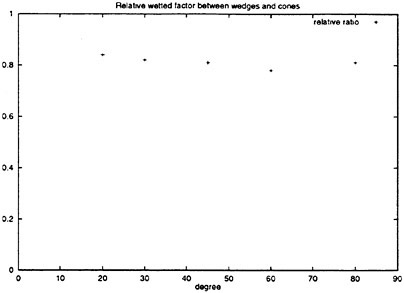
Figure 10: The ratio of the wetted factor between the axisymmetric cones and the two-dimensional wedges. The fully nonlinear theory is used. The vertical axis is the wetted factor Cw which is defined in equation (16).
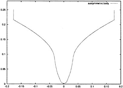
Figure 11: Geometry of an axisymmetric body with the geometry based on a two-dimensional bow flare section of a ship.
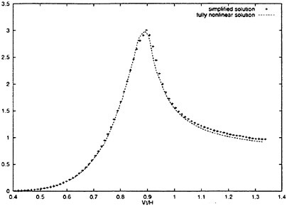
Figure 12: Total slamming force F3 of an axisymmetric body with the geometry based on a two-dimensional bow flare section of a ship. The flow separated at the knuckle. The fully nonlinear and simplified solutions are used. The vertical axis is F3/(ρV2H2). Η is the vertical distance between the keel and the knuckle, ρ, V and t are difined in figure 7.
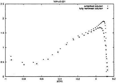
Figure 13: See caption on p. 662.

Figure 13: Slamming pressure p of an axisymmetric body with the geometry based on a two-dimensional bow flare section of a ship at instance Vt/H=0.631, Vt/H=0.688 and Vt/H=0.788. H is the vertical distance between the keel and the knuckle. The vertical axis is (p−pa)/(0.5ρV2). ρ, pa, z, V and t are difined in figure 7.
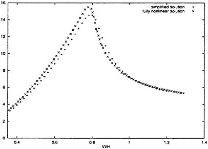
Figure 14: Numerical results of total slamming force of cones with deadrise angle 30°. The flow separated at the knuckle. The fully nonlinear and simplified solutions are used. The vertical axis is F3/(ρV2H2). Η is the vertical distance between the keel and the knuckle, ρ, V and t are difined in figure 7.
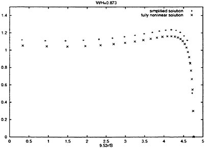
Figure 15: See caption on p. 663.
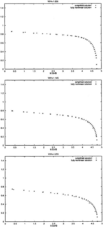
Figure 15: Numerical results of total slamming pressure of cones with deadrise angle 30°. The flow has separated at the knuckle. The instances Vt/H=0.873, 1.036, 1.145 and 1.291 are plotted. The fully nonlinear and simplified solutions are used. The vertical axis is (p−pa)/(pV2). Β is the maximun diameter of the cone. Η is the vertical distance between the keel and the knuckle, r is defined in figure 1. ρ, pa, V and t are difined in figure 7.
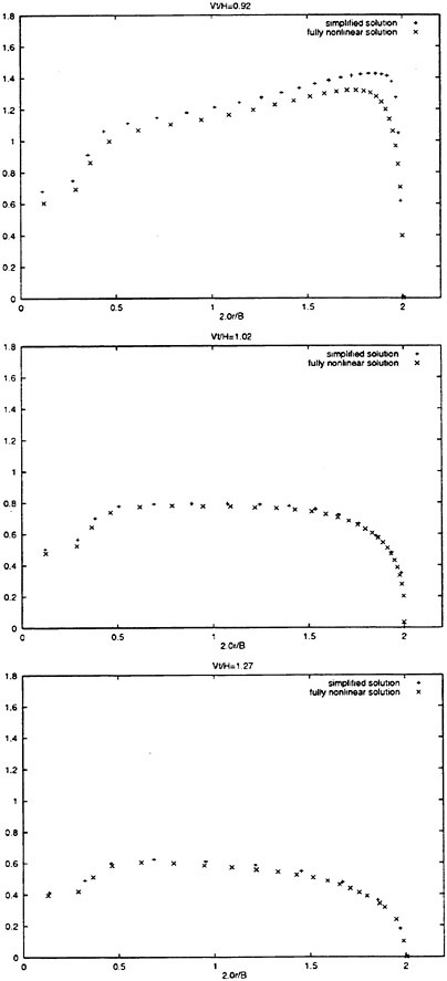
Figure 16: Numerical results of total slamming pressure on an axisymmetric body with the geometry based on a two-dimensional bow flare section of a ship. The flow has separated at the knuckle. The fully nonlinear and simplified solutions are used. The vertical axis is (p− pa)/(ρV2). B is the maximum diameter of the body. H is the vertical distance between the keel and the knuckle, r is defined in figure 1. ρ, pa, V and t are difined in figure 7.
DISCUSSION
U.Bulgarelli
Istituto Nazionale per Studi ed Esperienze di Architettura Navale, Italy
-
Do the number of panels of the submerged part affect the solution?
-
What does “particular care in moving the free surface to conserve the mass” mean?
AUTHORS’ REPLY
In our numerical calculation the number of elements on the wetted surface is kept constant, so the submergence will not affect the solution. Because we used lower order panel method, special care has been taken in order to satisfy the conservation of mass. That means that the rate of change with time of the water volume above z=0 should be equal to the rate of change with time of the body displacement below z=0. A detailed discussion about it can be found in Zhao and Faltinesen (1993).
DISCUSSION
D.Clarke
University of Newcastle Upon Tyne, United Kingdom
In two-dimensional flow, if you consider planing action, then the momentum change in the jet of fluid thrown forward is proportional to the normal force on the planing surface. In this three-dimensional case, can this fact not be used to define the cut off of the jet, where it is considered as one-dimensional flow?
AUTHORS’ REPLY
The two-dimensional planing problem is a steady state problem, which is different from the slamming problem. It can be shown that the momentum change in the jet can be neglected in the calculation of slamming force for asymptotically small deadrise angle (in using the conservation of momentum to predict slamming force).
Ref.
Zhao, R. and Faltinsen, O. “Water entry of two-dimensional bodies,” Journal of Fluid Mechanics, Vol. 246, 1993.
DISCUSSION
L.Adegeest
Det Norske Veritas, Norway
Did you compare the 3D results with the results of your earlier published 2D method? I’m asking you this question because the 2D method can easily be applied to ship-forms by applying a ship-wise discretization. Probably it is not possible to do the same with this extreme 3D example, but it should be possible to compute a “2D” force by interpolating the 2D pressure distribution, to be calculated for the vertical symmetry plane, over the cone according to
where c is the contour of the symmetry plane.
It would be very interesting and relatively easy to quantify the 3D effect this way. Or is it maybe the same?
AUTHORS’ REPLY
We have done the comparison of slamming pressure between a 2D wedge and a cone for different deadrise angles. The results of pressure distribution for the cones are presented in figure 7. The results for the wedges are given by Zhao and Faltinesen (1993). For small deadrise angle the maximum pressure is dependent on the wetted factor in square. Figure 10 shows the ratio of the wetted factor between the cones and wedges. The factor is dependent on the deadrise angles, which is about 0.8. That means that the maximum pressure for the cone is about 0.64 times the maximum pressure of the wedge with small deadrise angle. Increasing deadrise angle, this ratio will be changed. The ratio is about 0.72 for deadrise angle of 30 degrees. The average pressure for the cone is also lower than the average pressure of the wedge, which is also dependent on the deadrise angles. F2D=∝×F3D×∝.