
Applications of Recursive Neural Network Technologies to Hydrodynamics
W.Faller, D.Hess, W.Smith, T.Huang
(Naval Surface Warfare Center, Carderock Division, USA)
ABSTRACT
Recursive neural networks (RNNs) are a technique for developing time-dependent, nonlinear equation systems. Simulation tools based on RNNs have been developed which may assist in addressing a wide range of submarine and ship hydrodynamic maneuvering and control challenges. Faster than real-time, six degree-of-freedom (6-DOF) maneuver simulations have been developed for both full scale and model scale submarines using RNNs combined with model scale and full scale trials maneuvering data. The simulations show no appreciable loss of fidelity in predicting severe or emergency recovery procedure maneuvers which include rapid propeller rotation reversal. The results indicate that the RNN simulations provide accurate predictions for submarine maneuvers used to develop the simulations as well as for validation maneuvers. For hundreds of submarine maneuvers, full scale and model scale, the average simulation errors in depth are less than 3 m (full scale), less than 0.25 kts in speed (full scale), and less than one degree in pitch angle and roll angle. Consistent results were obtained across all maneuver types including crashbacks, rise jams, dive jams, rudder jams, turns, vertical and horizontal overshoots. Currently, these simulation tools are being implemented for surface ship maneuvers. In addition, full scale simulations provide the opportunity to eliminate Reynolds number scaling issues from the simulation of submarine maneuvers. Further, the capability to generate simulations of the equivalent full scale and model scale vehicle has provided a number of opportunities for studying the physics underlying vehicle maneuvering. For example, RNN simulations indicate that variations in roll dynamics (roll angular rate and roll angular acceleration) contribute significantly to the observed differences between model scale and full scale submarine maneuvers for emergency recovery procedures. Results from RNN simulations have also provided new insights into the physics of the three-dimensional unsteady vortex dominated flow fields which govern the vehicle maneuvers. For six degree-of-freedom problems, traditionally, dynamic similarity has been obtained by nondimensionalizing all variables as a function of a characteristic length (L) and the initial speed U0. However, RNN results indicate that dynamic similarity for maneuvering vehicles should be based on the time varying velocity U(t) and not U0.
NOTATION
|
CB |
Center of Buoyancy |
|
CG |
Center of gravity |
|
BG |
Distance from CB to CG |
|
L |
Body length, LOA (m) |
|
Lstn |
Length CG to control surfaces (m) |
|
Dp |
Propeller Diameter (m) |
|
U |
Total velocity (m/sec) |
|
|
Euler angles (rads) |
|
x, y, z |
Displacements (m) |
|
u, v, w |
Linear velocities (m/sec) |
|
|
Linear accelerations (m/sec2) |
|
p, q, r |
Angular velocities (rad/sec) |
|
|
Angular accelerations (rad/sec2) |
|
α |
Angle-of-attack tan−1(w/u) |
|
β |
Sideslip angle sin−1(−v/U) |
|
δb |
Bowplane deflection angle |
|
δr |
Rudder deflection angle |
|
δs |
Sternplane deflection angle |
|
RPM |
Propeller RPM |
|
Re |
Reynolds number |
|
f |
frequency (Hz) |
|
ω |
2πf |
|
k |
reduced frequency, Lω/2U∞ |
|
t |
real-time |
|
Δt |
real-time increment (tj+1−tj) |
|
t′ |
nondimensional time |
|
Δt′ |
nondimensional time step (t′j+1−t′j) |
INTRODUCTION
Results derived from a decade of free-flight model maneuvering data, on undersea vehicles, have demonstrated that time and spatially dependent unsteady fluid dynamic effects are large, extremely significant, and must be accounted for when predicting submarine maneuvers and controllability characteristics. In addition, this problem is accentuated by maneuvers which include reverse RPM
on the propeller. Further, results from both free-flight model maneuvering data and full scale trial maneuvering data, have failed to provide a quantitative determination of the scaling differences between model and full scale maneuvers. A number of possible sources for these differences between model scale and full scale exist and include, Reynolds number scaling issues, experimental errors, differences in the wetside geometry, variations in mass and moments of inertia, as well as variations in the distance (BG) between the center of buoyancy and the center of gravity.
A determination of the reasons underlying the observed maneuvering differences are complicated by the unsteady fluid dynamics which govern a majority of the vehicle motions. The fluid dynamics for a submarine are characterized by relatively large, time-varying combined angles-of-attack (α) and sideslip angles (β). The maneuvers also appear to be strongly influenced by forced unsteady fluid mechanics. The maneuvering vehicle is characterized by pitch and yaw angular rates (q, r) as well as angular accelerations ![]() which yield significant values for the reduced frequency parameter (k). Consistent with standard conventions the length constant used to determine (k) was half the boat length (L/2). To analytically estimate the reduced frequency of the maneuvering submarine, representative cases were approximated as harmonic motions.1 To simplify the analysis, the period of the motion (τ) was calculated using a sawtooth wave which is dependent on only the pitch and yaw angular rates. The frequency (f) for the harmonic motion was calculated as 1/τ. For simplicity, the mean amplitude αm was taken to be zero in all cases and only pure pitching or yawing conditions were calculated. Oscillation amplitudes of 5, 10 and 20 degrees, and RCM pitch and yaw rates of 0.5, 2 and 4 deg/sec were assumed. The estimates for the pitch and yaw rates were intentionally conservative so as to underestimate, rather than overestimate, the reduced frequency (k). This approximation is shown schematically in Figure 1. As shown, if the oscillation amplitude αω is halved, the period is halved and the corresponding frequency is doubled. Figure 2 summarizes the range of reduced frequencies as a function of speed (U) obtained from this analysis.
which yield significant values for the reduced frequency parameter (k). Consistent with standard conventions the length constant used to determine (k) was half the boat length (L/2). To analytically estimate the reduced frequency of the maneuvering submarine, representative cases were approximated as harmonic motions.1 To simplify the analysis, the period of the motion (τ) was calculated using a sawtooth wave which is dependent on only the pitch and yaw angular rates. The frequency (f) for the harmonic motion was calculated as 1/τ. For simplicity, the mean amplitude αm was taken to be zero in all cases and only pure pitching or yawing conditions were calculated. Oscillation amplitudes of 5, 10 and 20 degrees, and RCM pitch and yaw rates of 0.5, 2 and 4 deg/sec were assumed. The estimates for the pitch and yaw rates were intentionally conservative so as to underestimate, rather than overestimate, the reduced frequency (k). This approximation is shown schematically in Figure 1. As shown, if the oscillation amplitude αω is halved, the period is halved and the corresponding frequency is doubled. Figure 2 summarizes the range of reduced frequencies as a function of speed (U) obtained from this analysis.
Clearly, based on this analysis a majority of maneuvers have large reduced frequencies (k≫0.1). This indicates that the vehicle motion drives the development of the unsteady separated flow field. The vortical flow field, in turn, gives rise to the forces generated on the hull during these maneuvers. Further, under these conditions, Reynolds number is known to have only a second order effect on the flow field development. For a limited range of data, experiments support this contention.2
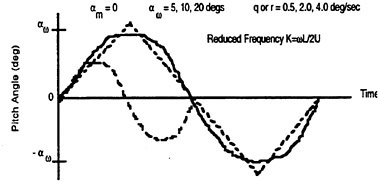
Figure 1. Submarine maneuvering approximated as a harmonic motion
|
|
αω=5 deg |
αω=10 deg |
αω=20 deg |
|
Gentle Maneuver 0.5 deg/sec |
k=0.67/U U=7 k=0.1 |
k=0.33/U U=7 k=0.05 |
k=0.17/U U=7 k=0.02 |
|
Intermediate 2.0 deg/sec |
k=3.34/U U=7 k=0.48 |
k=1.67/U U=7 k=0.24 |
k=0.84/U U=7 k=0.12 |
|
Severe Maneuver 4.0 deg/sec |
k=6.7/U U=7 k=0.96 |
k=3.35/U U=7 k=0.48 |
k=1.67/U U=7 k=0.24 |
Figure 2. Reduced frequencies (k) for the RCM during maneuvering.
Accordingly, development of simulation methodologies capable of representing unsteady separated flows is of paramount importance if new maneuver simulation tools are to be developed. Prior work indicates that, across an extremely broad range of parameters, both steady and unsteady fluid mechanics can be modeled using recursive neural networks. Techniques have also been addressed for integrating these unsteady fluid dynamic RNN simulations with mechanical actuators to demonstrate the ease with which adaptive control systems might be produced.
Recursive neural network simulations of unsteady boundary layer development, dynamic stall and dynamic reattachment for three-dimensional unsteady separated flow fields have been described.3−7 Further, techniques have been examined for integrating these recursive neural network (RNN) reference models within adaptive control systems. Overall, the results clearly demonstrated that RNNs are a highly effective technique for the time-dependent simulation of three-dimensional unsteady separated flow fields.3−7 Operationally, the unsteady flow-field wing interactions could be predicted for any time period over which the motion history was a known function (a few milliseconds to tens of seconds). Consistent with numerous experimental
investigations, the simulation results clearly demonstrate that the interactions between the body and the unsteady flow field are highly repeatable. For the neural network controller, the results indicated that unsteady aerodynamic processes can be controlled across a range of unsteady motion histories.6
The successful extension of these RNN technologies to submarine six degree-of-freedom maneuver simulation is the subject of this paper. The work described, herein, demonstrates the capability to use RNN maneuver simulations to provide direct simulations of full scale submarines, to independently simulate model scale submarines, and to use the combination of simulations to facilitate a quantitative determination of the scaling differences observed between model scale and full scale submarine maneuvers.
METHODS
Recursive Neural Networks
Recursive neural networks (RNNs) are a technique for developing time-dependent, nonlinear equation systems. The basic RNN architecture is comprised of an input vector or layer, hidden layer(s) and an output layer as shown in Fig. 3. Each layer is comprised of a set of units or processing elements at which information is processed. Information processing proceeds from left to right, with each input vector yielding a corresponding output vector. Recursive connections, or recurrent feedback, are utilized where the predicted outputs become part of the next input vector. By adding recurrence between the input and output layers time-dependence can be incorporated within the RNN solution.
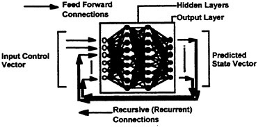
Figure 3. Overview of the recursive neural network architecture for maneuvering simulation.
Information processing within each layer of the RNN occurs at many simple processing units or elements, each of which is described by an activation function. The activation function determines the input-output relationships of each processing unit. The sigmoidal activation function described in Eqn. 1 is perhaps the most common nonlinear activation function, and is the activation function utilized in all the RNN maneuver simulations. As shown, the output of the activation function (y) is a function of the input (x).
(1)
Each processing unit is connected to other processing units via adjustable weights (coefficients). Typically, the number of processing units in the input and output layers are defined by the problem, whereas the number of hidden layers as well as the number of processing units per hidden layer is user defined. For a fully connected RNN, each processing unit in one layer connects to every processing element in the next layer. The input (x) to a processing element is described by Eqn. 2, and the corresponding output (y) of that processing element is given by Eqn. 1. For each unit, the output side (y) is defined by the subscript (i) and the input side (x) by the subscript (j). This process is carried forward from the input vector to the hidden layer(s) and from the hidden layer(s) to the output layer. Thus, the input vector is transformed nonlinearly into an output vector. The relative ease with which coupled time-dependent, nonlinear input-output relationships can be calculated is one of the significant strengths of the RNN approach. However, to utilize this capability requires a method, the learning algorithm, for adjusting the weights (coefficients) connecting the processing units such that a given time history of input vector yields the correct predicted output time history.
(2)
The RNN weights are adjusted by presenting a sequence of training vectors (inputs) to the RNN and calculating the RNN outputs. Since the error is the difference between the target (measured) values and the RNN predicted values, this process requires data sets where both the input and output vector time histories are known. The calculated error is then backpropagated, using a gradient descent method, to adjust the weights such that the error will be minimized. By iteratively repeating this process over a number of input-output data sets the weights can gradually be adjusted such that the RNN becomes an accurate time dependent, nonlinear transfer function between the input and output time histories.
Once the RNN training is complete, the final weights (coefficients) are fixed. For a fully
converged solution, the accuracy of the RNN simulation can then be judged in one of three ways. For a parameter space (x,y) to be simulated, training data would consist of a limited set of (x,y) pairs. Following training, the prediction accuracy can first be tested for data sets on which the neural network was trained. Second, the RNN predictions can be checked for cases which are within the parameter space, but which were not used during training. Thus, the RNN capability to generalize (interpolate) within the parameter space can be determined. Since neural networks are typically designed to operate within a predefined parameter space, this is the most critical test and is often used to validate the final RNN solution. Third, RNN predictions can also be tested against data sets which are outside of the training parameter space. Thus, the RNN capability to generalize (extrapolate) outside of the parameter space can be tested. The limitation on testing RNN extrapolation, as well as extrapolation for other simulation techniques, typically occurs because the experimental data sets required for comparison do not exist.
Recursive Neural Network Solutions
Recursive neural networks are a method for developing time-dependent, nonlinear equations which describe the behavior of complex systems. As a framework within which to consider the RNN solution, assume as a starting point a linearized state equation where the output vector of the equation system might be the vehicle dynamics. If the control variables are described by a vector ![]() and the state vector by
and the state vector by ![]() then
then ![]() can be calculated as given by Eqn. 3. Further, each state vector
can be calculated as given by Eqn. 3. Further, each state vector ![]() is a function of the prior states and control inputs as given in Eqn. 4.
is a function of the prior states and control inputs as given in Eqn. 4.
(3)
(4)
However, for complex nonlinear problems, a solution of this form typically cannot account for all of the underlying physics which would be required to achieve an exact solution. As such, each predicted state vector ![]() will include some error. This error can be defined as the difference between what the mathematical simulation predicts and what the actual measured response of the physical system would be to the same control inputs. Not surprisingly, as the vehicle maneuvers to be simulated become increasingly more complex the magnitude of the error terms tend to increase. These error terms can be accounted for in the mathematical solution by rewriting the state vector as a function of the predicted state
will include some error. This error can be defined as the difference between what the mathematical simulation predicts and what the actual measured response of the physical system would be to the same control inputs. Not surprisingly, as the vehicle maneuvers to be simulated become increasingly more complex the magnitude of the error terms tend to increase. These error terms can be accounted for in the mathematical solution by rewriting the state vector as a function of the predicted state ![]() plus the error term ēj+1. This new state vector can be denoted as ŷj+1, Eqn. 5, and the corresponding state equation as shown in Eqns. 6 and 7. For simplicity, the assumption is that errors in the predicted states do not change the control inputs. Clearly, this would not be the case if a feedback control system was being utilized.
plus the error term ēj+1. This new state vector can be denoted as ŷj+1, Eqn. 5, and the corresponding state equation as shown in Eqns. 6 and 7. For simplicity, the assumption is that errors in the predicted states do not change the control inputs. Clearly, this would not be the case if a feedback control system was being utilized.
(5)
(6)
(7)
Further, since the error terms are not independent of each other, one difficulty encountered with such solutions is that as a first approximation the error term ēj+1 can roughly be assumed to sum or accumulate over time. As such, the error in the final state vector ŷn can be approximated by the total error (E) given in Eqn. 8. In general, this total error (E) increases proportionally as a function of both the complexity of the vehicle maneuver to be simulated and the maneuver duration (length of time).

(8)
Further, since ŷj+1 may correspond to the vehicle accelerations, the integration of the acceleration terms, which include the error ēj+1 at each time step, yield vehicle velocities which typically have correspondingly larger errors than the accelerations. In turn, the subsequent integration of the velocities to yield the vehicle trajectory and attitude can further magnify the differences which may be observed between the simulation predicted and the measured response of the vehicle. The same difficulties exist for simulations which directly calculate the forces and moments and then solve for the accelerations.
While the matrices A and Β are not separate in the RNN, for the purpose of discussion, the RNN solution can be considered to have the form shown below. The control vector ûj is also a function of the state vector ŷj and is given by Eqn. 9. For the RNN, the A and Β matrices also vary as a function of time, and are a function of both the control vector ûj and the state vector ŷj as given by Eqn. 10. The predicted state vector ŷj+1, in turn, is a nonlinear function of
these time-varying matrices and input vectors as given by Eqn. 11.
(9)
(10)
(11)
A critical issue in simulation is that, for all practical purposes, an exact solution which would have error terms ēj+1 equal to zero does not exist. As such, simulation fidelity is dependent not only on predicting the state vector, but perhaps more importantly on effectively dealing with and minimizing the predicted error terms ēj+1. A significant advantage, which intentionally has been built into the RNN paradigm, is that the RNN equation system can be developed such that ŷj+1 is the correct predicted state. In other words, the RNN equation system can operate in a fashion where the correct predicted state is the measured value ![]() plus a small error ēj+1. The error may, or may not be, zero at any time step. However, as long as the error remains small, the RNN simulation, for all intents and purposes, predicts the state vector
plus a small error ēj+1. The error may, or may not be, zero at any time step. However, as long as the error remains small, the RNN simulation, for all intents and purposes, predicts the state vector ![]() that would correspond to the measured response of the physical system to the same control inputs. As such, unlike other solutions, as a first approximation the predicted error terms for a converged solution do not integrate over time. The total error (E) for an RNN simulation typically has a magnitude similar to the magnitude of the predicted error at any time step ej, Eqn. 12.
that would correspond to the measured response of the physical system to the same control inputs. As such, unlike other solutions, as a first approximation the predicted error terms for a converged solution do not integrate over time. The total error (E) for an RNN simulation typically has a magnitude similar to the magnitude of the predicted error at any time step ej, Eqn. 12.
(12)
This is significant because any error in the predicted state vectors is both small and roughly a constant over time. Further, in general, the errors in the state vectors do not increase as a function of the complexity of the vehicle maneuver or the maneuver duration. In addition, as discussed elsewhere1, since ŷj+1 within the RNN simulation can correspond to the six state variables (linear velocities and angular rates), the subsequent integration to yield the vehicle trajectory and attitude typically results in relatively small differences between the RNN simulation predictions and the measured response of the vehicle. As described below, across hundreds of submarine maneuvers, full scale and model scale, RNN simulations yield errors in depth which on average are less than 3 m (full scale), less than 0.25 kts in speed (full scale), and less than one degree in pitch angle and roll angle.
Experimental Data
Submarine maneuvers have been obtained from two sources; full scale submarine trials and free-flight radio controlled model (RCM) experiments. Full scale submarine trials have the advantage that no scaling issues need to be addressed. However, as described below, three of the state variables (u, v and w) must be estimated since no direct measurements are typically available. The RCM can provide a much broader set of measurements, including forces and moments on both the control surfaces and propeller, but maneuvering differences due to scaling issues between model scale and full scale must then be addressed. The Reynolds number is approximately 107 for the RCM based on total body length versus 109 for the equivalent full scale submarine.
The RCM was designed to provide an experimental testbed for determining the steady and unsteady fluid mechanics effects of vehicle maneuvering. The RCM is scaled from the full scale vehicle based on the linear scale ratio of the vehicle lengths (Lship/Lmodel). Using the RCM, a full range of motion and control measurements are available across all maneuver types. Figure 3 depicts the basic RCM functional arrangement. Data is collected from on board sensors which include vertical reference gyros, linear and angular accelerometers. All sensor data is digitized and stored either on board or telemetered to shore in real time via a Pulse Code Modulated data up-link. In addition to the on board data sensors an external acoustic tracking system is used to provide x, y, z tracking of the time-varying displacements (trajectory) of the model. A detailed explanation of the experimental system including both the onboard instrumentation as well as the acoustic tracking system has previously been provided.8 Figure 4 shows the reference coordinate system (right-hand rule) with (z) being positive downwards. Table 1 summarizes the experimental and analytically derived six degree-of-freedom (6-DOF) data obtained for a maneuvering vehicle.
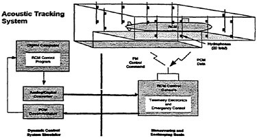
Figure 3. Overview of RCM operation in the Maneuvering and Seakeeping Basin (MASK).
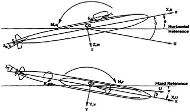
Figure 4. Reference coordinate system
Table 1. Data obtained for six degree-of-freedom maneuvers
|
U |
(Total velocity) |
|
|
(Linear vels and accels) |
|
|
(Angular vels and accels) |
|
|
(Euler angles) |
|
x, y, z |
(Displacements) |
To develop the RNN maneuver simulations, the 6-DOF state variables [u, v, w, p, q, r] as well as the accelerations ![]() the time-varying Euler angles
the time-varying Euler angles ![]() and the trajectories [x, y, z] were obtained from the RCM during severe maneuvers.8 In addition, maneuvering data were obtained from full scale submarine trials. To utilize the full scale trials data the three state variables (u, v, w) were estimated using a set of three feed forward neural networks.
and the trajectories [x, y, z] were obtained from the RCM during severe maneuvers.8 In addition, maneuvering data were obtained from full scale submarine trials. To utilize the full scale trials data the three state variables (u, v, w) were estimated using a set of three feed forward neural networks.
Full scale trials conducted in the open ocean are able to accurately measure depth (z), speed (U), the Euler angles (φ, θ, ψ), and the angular velocities (p, q, r). The angular accelerations may be derived from the measured data. However, measurements of the trajectory (x, y), the linear velocities (u, v, w), and accurate measurements of the linear accelerations ![]()
![]() are unavailable. The RCM provides accurate measurements of the depth (z), speed (U), the Euler angles (φ, θ, ψ), and the angular velocities (p, q, r). In addition, the RCM is operated in a facility equipped with an acoustic tracking system which permits accurate time histories of the trajectory (x, y) to be obtained during each maneuver. Since measured trajectory data and depth are available, the linear velocities (u, v, w) as well as the linear accelerations
are unavailable. The RCM provides accurate measurements of the depth (z), speed (U), the Euler angles (φ, θ, ψ), and the angular velocities (p, q, r). In addition, the RCM is operated in a facility equipped with an acoustic tracking system which permits accurate time histories of the trajectory (x, y) to be obtained during each maneuver. Since measured trajectory data and depth are available, the linear velocities (u, v, w) as well as the linear accelerations ![]() may be derived for the RCM. This data is then used to train feed forward neural networks to predict the linear velocity components as a function of variables which are measured at both model scale and full scale. The technique results in a set of three nonlinear equations, feed forward neural networks, which can be used to decompose the total velocity (U) into the three linear velocity components.
may be derived for the RCM. This data is then used to train feed forward neural networks to predict the linear velocity components as a function of variables which are measured at both model scale and full scale. The technique results in a set of three nonlinear equations, feed forward neural networks, which can be used to decompose the total velocity (U) into the three linear velocity components.
Specifically, three neural networks are utilized for the prediction of u, v and w, respectively. In each case, the input variables are U, q, r, φ and θ which are variables that are measured for both RCM and full scale maneuvers. The predicted neural network output is u, v or w. This is shown schematically in Fig. 5. Each of the three networks is trained using RCM data for which both the inputs and outputs are known. Post-training, the trained neural networks can then be used with full scale data as the inputs to provide time histories for the full scale linear velocities (u, v, w). In this manner, the feed forward neural networks can serve as virtual sensors for the estimation of u, v and w for the full scale trials data.
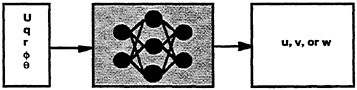
Figure 5. Feed forward neural network used to estimate the linear velocity components for full scale maneuvers. One neural network is constructed for each velocity term u, v, and w, respectively.
After predictions for u, v and w have been acquired, the velocity magnitudes can be refined using known mathematical relationships between measured and predicted values. Although no tracking system is available to provide x and y, depth, z, is measured during full scale trials by means of pressure sensors.
Therefore, the predicted velocity components u, v, and w are transformed from the body coordinate system to the inertial coordinate system using a direction cosine matrix formed using the measured Euler angles and then integrated to obtain predictions for x, y, and z. Then, the measured time history for z is substituted in place of the predicted depth and the process is reversed to obtain revised predictions of u, v, and w. These corrections are small with the largest correction in the w component. The overall speed of the vehicle U is also a measured quantity. Since, among the velocity components the largest contributor to U is u, we can use Umeas to further improve the u component prediction as given in Eqn. 13.
(13)
Further, these steps ensure that the u, v and w estimates are mathematically consistent with those measured full scale variables that exist. The minor corrections introduced by this refinement process have enhanced the u and w predictions at the expense of the v prediction; any remaining error is expected to be in the v component. A second correction algorithm which permits the error in lateral velocity (v) to be corrected is currently under development.
Prior to the refinement procedure, the ability of the neural networks to predict the linear velocities can be judged using RCM data. The following steps were carried out for each of the three neural networks. After obtaining a predicted value from a neural network at a given time step, the predicted and measured values are scaled to full scale magnitudes and then several error measures are computed at each time step. The error measures at each time step are then averaged over all of the time steps during the course of the maneuver. Representative error measures for each neural network are given in Table 2. In each case, the average angle measure (AAM) is quite close to 1.0 indicating that the comparison of the relative shapes and magnitude of the predicted and measured time histories for each velocity component is excellent. The absolute errors are reported in m/sec and correspond to full scale values. Again, the results indicate that the neural networks provide accurate estimations of the linear velocity components u, v and w.
Table 2. Neural network predictions, prior to the refinement procedure. All error values are full scale.
|
|
AAM |
Absolute Error |
|
u |
1.00 |
0.01 m/sec |
|
v |
0.98 |
0.03 m/sec |
|
w |
0.95 |
0.03 m/sec |
Representative errors for the linear velocity components after the refinement process are given in Table 3. Again, the absolute errors are reported in m/sec and correspond to full scale values. The results indicate that the refined estimates provide improved predictions for u and w, without significantly changing the prediction of v. The post refinement linear velocity components are used to complete the full scale trials maneuvering data.
Table 3. Neural network predictions, after the refinement procedure. All error values are full scale.
|
|
AAM |
Absolute Error |
|
u |
1.00 |
0.01 m/sec |
|
v |
0.98 |
0.03 m/sec |
|
w |
1.00 |
0.01 m/sec |
Overall, the method described provides an accurate, mathematically consistent and reliable means for estimating the remaining three state variables which are required for a complete description of the six degree-of-freedom motion. The accuracy of these estimates, as judged by the ability to recover the known full scale measurements ![]() is excellent. Further, this technique enables the use of full scale trials data for the development of RNN simulations of full scale submarine maneuvers. The full scale RNN simulation results, described below, indicate that the accuracy of this method is sufficient to permit accurate simulations of full scale submarines to be developed.
is excellent. Further, this technique enables the use of full scale trials data for the development of RNN simulations of full scale submarine maneuvers. The full scale RNN simulation results, described below, indicate that the accuracy of this method is sufficient to permit accurate simulations of full scale submarines to be developed.
Application Of RNNs To Maneuver Simulation
Figure 6 schematically shows the RNN 6-DOF maneuver simulation. To function as a maneuver simulation requires that the only external inputs to the RNN be the time-varying control signals and the initial conditions at time (t0). The inputs (controls) were the propeller RPM, the rudder deflection angle, the sternplane deflection angle(s) and the bowplane deflection angle. The component force
modules, described in more detail below, act on these controls and provide the inputs, as forces, to the RNN. The predicted outputs are the time-varying 6-DOF state variables [u, v, w, p, q, r]. To model the time-dependence of the vehicle dynamics, which is reflective of the time-dependence of the unsteady fluid mechanics, the predicted outputs (state variables) were recursed, fed back, as inputs to the RNN throughout the vehicle motion history. The accelerations ![]() the Euler angles
the Euler angles ![]() and the trajectories [x, y, z] are calculated internally. Further, as described below, the RNN simulations are based on a novel formulation of dynamic similarity.
and the trajectories [x, y, z] are calculated internally. Further, as described below, the RNN simulations are based on a novel formulation of dynamic similarity.
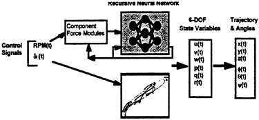
Figure 6. The RNN six degree-of-freedom maneuvering simulation. The inputs to the RNN are the propeller RPM and plane deflection angles. The RNN outputs are the six state variables (u, v, w, p, q, and r) from which the displacements (trajectory) and angles can be derived.
For six degree-of-freedom maneuver simulations, traditionally, dynamic similarity has been obtained by nondimensionalizing all variables as a function of a characteristic length (L) and the initial speed U0. However, the known physics of unsteady fluid mechanics suggests that to maintain dynamic similarity for maneuvering vehicles all variables, including time, should be nondimensionalized based on the time-varying velocity U(t), rather than U0. The reasons for this can be summarized as follows. The reduced frequency for the majority of maneuvers is large (k≫0.1). The forces which, in turn, determine the accelerations predominantly result from the interaction between the far field, three-dimensional vortical flow field and the surface of the hull. The vehicle can change speed drastically during a maneuver. The redistribution of vorticity in the far field is governed by convective fluid motions, and convective fluid motions scale as a function of the time-varying velocity U(t) and not the initial speed U0. The general solution for dynamic similarity can be shown to be based on U(t).1 Dynamic similarity based on U0 is a special case of the general solution, and occurs when U(t) equals a constant. As such, a new formulation of dynamic similarity was developed for the RNN simulations based on the time-varying velocity U(t).
Further, analyses based on RNN maneuver simulations support the contention that dynamic similarity should be based on U(t). If one compares the three possible forms of solutions which can be derived for RNN simulations; (1) simulations based on real-time, (2) simulations based on scaling all variables using U0, and (3) simulations based on scaling all variables using U(t) the following results are observed for the simulation predictions of the vehicle maneuvers. Simulations based on real-time are of poor fidelity. Simulations based on dimensionless variables calculated using U0 are limited to good simulation fidelity for maneuvers which all have, within some finite range, the same initial speed U0. This problem is accentuated by maneuvers which involve reverse RPM on the propeller. Simulations based on dimensionless variables calculated using U(t) show good simulation fidelity across all maneuvers, including maneuvers which have negative RPM on the propeller. The calculation of dynamic similarity, based on U(t), includes both nondimensional time as well as the nondimensionalization of all other variables and is summarized below.
For reference, nondimensional time is traditionally calculated as shown in Eqn. 14. This of course, assumes that the velocity of the vehicle does not change. While initially it may seem that the formulation for nondimensional time based on U(t) would be given by Eqn. 15, this does not turn out to be the case. Since within the simulation the nondimensional time-step Δt′ must be equal to a constant, the problem which occurs is that time, as well as nondimensional time, must sequentially march forward into the future. However, if during a maneuver the value of U(t) decreases rapidly it is quite possible to get the following situation ![]() the calculated value is smaller than the previously calculated value of nondimensional time, an unacceptable situation. Therefore, nondimensional time based on U(t) must be formulated as shown in Eqn. 16. The conversion back to real time is given by Eqn. 17. Note, the traditional form of nondimensional time given by Eqn. 14 is a special case of Eqns. 16 and 17 and occurs when U(j) equals a constant. The critical issue for dynamic similarity, in time, is that Δt′ must always be equal to a constant. Therefore,
the calculated value is smaller than the previously calculated value of nondimensional time, an unacceptable situation. Therefore, nondimensional time based on U(t) must be formulated as shown in Eqn. 16. The conversion back to real time is given by Eqn. 17. Note, the traditional form of nondimensional time given by Eqn. 14 is a special case of Eqns. 16 and 17 and occurs when U(j) equals a constant. The critical issue for dynamic similarity, in time, is that Δt′ must always be equal to a constant. Therefore, ![]() must always be equal to a constant. To reiterate, the general formulation for dynamic similarity, in time, which captures the known physics of the problem, is given in Eqns. 16 and 17. For the RNN maneuver simulations, a nondimensional step size of Δt′ equal to 0.05 yields
must always be equal to a constant. To reiterate, the general formulation for dynamic similarity, in time, which captures the known physics of the problem, is given in Eqns. 16 and 17. For the RNN maneuver simulations, a nondimensional step size of Δt′ equal to 0.05 yields
accurate solutions for maneuver simulations in the speed range between 5 knots and flank speed (full scale). For lower speed maneuvers a smaller nondimensional step size, on the order of Δt′ equal to 0.0125 to 0.025, is required.
(14)
(15)
(16)
(17)
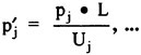
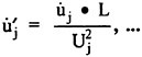
The same considerations apply to the nondimensionalization of the velocities and accelerations. To maintain dynamic similarity based on U(j) requires that the remaining variables be rendered dimensionless as shown in Eqns. 18–21. A more detailed description of this process, including the exact formulation required to implement these changes within the RNN simulation code, has previously been given.1
(18)
(19)
(20)
(21)
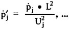
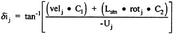
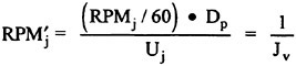
Control surface deflections which serve as inputs to the RNN were formulated as forces based on the effective or local angle-of-attack. For any control surface, the force Fj used as the input to the RNN is given in Eqn. 22. The induced angle-of-attack is determined from the local velocity (v or w) and the rotational rate (q or r) as shown in Eqn. 23. The full equations have previously been described in more detail.1 Critically, the coefficient values for C1-C3 can be set equal to one. This formulation, in general, yields the correct force time-history, but not necessarily the correct magnitude. If the force histories are known, then the coefficients required to match both the time history and magnitude can readily be determined. Further, this simple approximation appears to be adequate for both all moveable as well as flapped control surfaces. The RNN input term for the propeller force (RPM′) is given in Eqn. 24. The length constant (Dp) is the propeller diameter. The inputs to the RNN for the forces on the hull were based on the angle-of-attack and sideslip angle as given in Eqns. 25 and 26. The full details of the input terms, the RNN formulation as a 6-DOF solver, the RNN outputs and subsequent reconstruction of the trajectory and attitude predicted by the simulation have previously been described in detail.1
(22)
(23)
(24)
(25)
(26)
To train the RNN a subset of the available experimental data records, encompassing all maneuver types, were used to “teach” the neural network the relationship between the time-varying control signals and the time-dependent vehicle dynamics. The remaining data sets were used to validate the RNN simulation and demonstrate a general solution across all maneuvers. Following development, no additional changes were made to the RNN simulations; the weight matrices were fixed and the control inputs for both training and validation data sets were simply presented to the RNN 6-DOF maneuver simulation. The complete RNN equation system as well as the learning algorithms required for training the simulation are beyond the scope of this paper, but have previously been described in detail.1 Using this paradigm, both RCM and full scale submarine simulations have been constructed. Representative results for both model scale and full scale submarine simulations are described below.
In addition, for specific submarines, full scale and model scale simulations have been constructed for the same submarine. The full scale simulation(s), for these cases, were developed based on the full scale submarine trials maneuvering data. The model scale RCM simulation(s), for these cases, were developed using the RCM maneuvering data.
Following the development of the simulations, comparisons could then be drawn between any of the RNN simulation results and any of the maneuvering data from either full scale or model scale. This is shown schematically in Fig. 7. The RNN simulation of the full scale submarine can be compared to the full scale trials data, the model scale data or the model scale RNN simulation. Similarly, the RNN simulation of the model scale submarine can be compared to the model scale data, the full scale trials data or the full scale RNN simulations. Further, within the RNN maneuver simulation any of the control sequences or state variables can be manipulated. This permits new maneuvers to be studied, the effect of errors in the timing and/or magnitude of control sequences on the ensuing submarine maneuvers to be determined, and provides the opportunity to quantitatively study the scaling differences between model scale and full scale submarines.
In particular, for one such scaling study, the normally observed differences in the steady state roll angle could be matched between the RCM and full scale by altering the roll angle at time (t0) to match either the corresponding RCM or full scale roll angle ![]() . Thus, RCM simulations could be run with the full scale steady roll angle, and full scale simulations could be run with the RCM steady roll angle. These simulation results could then be directly compared to the experimentally measured maneuvers. Similarly, for the same study, any of the vehicle dynamics could be altered by changing the values within the simulation. For example, since the roll dynamics
. Thus, RCM simulations could be run with the full scale steady roll angle, and full scale simulations could be run with the RCM steady roll angle. These simulation results could then be directly compared to the experimentally measured maneuvers. Similarly, for the same study, any of the vehicle dynamics could be altered by changing the values within the simulation. For example, since the roll dynamics ![]()
![]() of the model scale vehicle are known at each time step, and correspond in a one-to-one fashion with the full scale roll dynamics
of the model scale vehicle are known at each time step, and correspond in a one-to-one fashion with the full scale roll dynamics ![]() one can readily substitute the model scale rolling behavior for the corresponding full scale values. In particular, the submarine roll angular rate and roll angular acceleration can be matched between the RCM and full scale by substituting the RCM roll dynamics
one can readily substitute the model scale rolling behavior for the corresponding full scale values. In particular, the submarine roll angular rate and roll angular acceleration can be matched between the RCM and full scale by substituting the RCM roll dynamics ![]()
![]() into the full scale simulation at each time step, and the full scale roll dynamics
into the full scale simulation at each time step, and the full scale roll dynamics ![]() into the RCM simulation at each time step. It should be noted, that this direct substitution approach is only applicable to correlation maneuvers where there is a one-to-one match in the control sequences and time histories of both the model scale and full scale submarine. Critically, these changes not only alter the roll characteristics, but effect the entire submarine dynamics by acting on the other variables
into the RCM simulation at each time step. It should be noted, that this direct substitution approach is only applicable to correlation maneuvers where there is a one-to-one match in the control sequences and time histories of both the model scale and full scale submarine. Critically, these changes not only alter the roll characteristics, but effect the entire submarine dynamics by acting on the other variables ![]() throughout the time history of the simulation. These simulation results can then be directly compared to the experimentally measured maneuvers. Thus, the effects of roll on full scale maneuvers as compared to RCM maneuvers can be directly determined. Similarly, the effects of roll on model scale maneuvers as compared to full scale maneuvers can be directly determined.
throughout the time history of the simulation. These simulation results can then be directly compared to the experimentally measured maneuvers. Thus, the effects of roll on full scale maneuvers as compared to RCM maneuvers can be directly determined. Similarly, the effects of roll on model scale maneuvers as compared to full scale maneuvers can be directly determined.
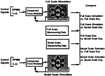
Figure 7. The RNN six degree-of-freedom maneuvering simulations. The full scale and model scale simulations can be compared directly to the experimental data and/or to the simulation results.
RESULTS
RNN Model Scale Simulation
The maneuvering simulation results, shown herein, were developed in two ways. First, one RNN 6-DOF simulation was developed for all maneuver types. Second, a single RNN 6-DOF simulation was separately developed for each individual maneuver type (crashbacks, rise jams, dive jams, rudder jams, turns, vertical and horizontal overshoots). The speed of these maneuvers ranged between 12 kts and flank speed. For each case, the results are categorized as errors for training, RNN development, data sets, and errors for the validation maneuvers which had not been previously “seen” by the simulation. As shown below, the full simulation compares favorably to the individual simulations, and indicates that only one RNN is required to provide an accurate simulation for all maneuvers.
To judge the accuracy of the simulation, all predicted and measured variables were co-plotted; velocities, accelerations, Euler angles, displacements and control signals. In addition, the following error measures were calculated for all variables; the absolute error in magnitude and the average angle measure (AAM) were calculated using the measured maneuvering data and the RNN simulation predictions. The average angle measure has a value of one in the best case, a perfect simulation of the maneuver, when the predicted and measured values are
exactly the same. Conversely, for very poor predictions, the average angle measure has a value of zero. The exception to this occurs when the signal is of small magnitude, near zero, for the average angle measure. The absolute error in magnitude was simply calculated as the absolute value of the difference between the measured and predicted values summed over each data point and then normalized by the number of data points. Since the predicted state variables are integrated to calculate the trajectory and attitude, the maximum error typically occurs at the end of each maneuver, and can be assumed to typically have a magnitude of roughly twice the absolute error in magnitude.
All of the model scale results have been scaled to the equivalent full scale distances, velocities or angles as appropriate. As such, all error measures were calculated based on the errors which would be expected for full scale submarine maneuvers. An error in depth of 3 meters, for example, is a full scale error not a model scale error. Herein, only the quantitative results based on the calculated error measures are given. All of these values are consistent with the plots, and indicate that the simulation predictions agree well with the experimentally measured data. For the roll angle, the low values obtained for the average angle measure can in part be attributed to a small offset, near zero, between the measured and predicted values. For these cases, the absolute error may be more representative of the true error observed between the predicted and measured roll angle.
Listed below are results computed over all data sets, for a typical submarine simulation. The maneuvers consisted of crashbacks, rise jams, dive jams, rudder jams, turns, vertical and horizontal overshoots. The results are summarized for training data sets in Table 4 and validation data sets in Table 5. The data set was comprised of a total of 250 maneuvers of which 184 were used to develop the RNN and 66 were used to validate the simulation. The results show that the RNN simulation accurately predicts the vehicle maneuvers. Across all 250 maneuvers, the average error in depth was less than 3 m (full scale), less than 0.25 kts in speed (full scale), and less than one degree in pitch angle and roll angle. However, the simulation is not perfect; of the 250 maneuvers roughly 5–10% of the predicted maneuvers scored measurably below the average values. Similarly, roughly 5–10% were predicted measurably better than the average values. Significantly, the results for data sets used to validate the simulation, Table 5, are consistent with the data sets used in development, Table 4. This indicates that the simulation, to the extent experimental data exists to compare with, is a general solution across all of the maneuvers.
Table 4. Simulation results for all maneuvers. Full scale error measures for the training data sets. (184 data sets)
|
|
AAM |
Absolute Error |
|
Speed (U) |
1.00 |
0.16 kts |
|
Roll Angle |
0.58 |
0.52 deg |
|
Pitch Angle (θ) |
0.83 |
0.93 deg |
|
Depth (z) |
0.98 |
2.29 m |
Table 5. Simulation results for all maneuvers. Full scale error measures for the validation data sets. (66 data sets)
|
|
AAM |
Absolute Error |
|
Speed (U) |
0.99 |
0.21 kts |
|
Roll Angle |
0.53 |
0.69 deg |
|
Pitch Angle (θ) |
0.83 |
1.12 deg |
|
Depth (z) |
0.97 |
2.47 m |
Representative results for single maneuver RNN simulations are given in Tables 6–9. The results for both controlled and uncontrolled crashbacks are given in Tables 6 and 7. The results for rise jams are shown in Tables 8 and 9. Consistent results were obtained for all other maneuver types. In each case, the number of data sets used to validate the simulation as well as the number of data sets used in development are given. These numbers vary and are a function of the available total number of data sets for each type of maneuver. The results show that each individual simulation accurately predicts the specific vehicle maneuver. In all cases, the results for data sets used to validate the simulation are consistent with the data sets used in development. As would be expected, in general, the results for the validation data sets indicate that the completely novel cases are not predicted quite as well by the RNN simulation as the training data sets. However, the differences do not appear to be significant. More importantly, the results for the full simulation, based on one RNN, compare favorably to the individual simulations. This indicates that a single RNN maneuver simulation can be used for all maneuvers.
Table 6. Simulation results for crashback maneuvers. Full scale error measures for the training data sets. (50 data sets)
|
|
AAM |
Absolute Error |
|
Speed (U) |
0.99 |
0.21 kts |
|
Roll Angle |
0.56 |
0.45 deg |
|
Pitch Angle (θ) |
0.83 |
1.16 deg |
|
Depth (z) |
0.97 |
2.60 m |
Table 7. Simulation results for crashback maneuvers. Full scale error measures for the validation data sets. (19 data sets)
|
|
AAM |
Absolute Error |
|
Speed (U) |
0.99 |
0.25 kts |
|
Roll Angle |
0.29 |
0.79 deg |
|
Pitch Angle (θ) |
0.77 |
1.30 deg |
|
Depth (z) |
0.97 |
3.17 m |
Table 8. Simulation results for rise jam maneuvers. Full scale error measures for the training data sets. (66 data sets)
|
|
AAM |
Absolute Error |
|
Speed (U) |
1.00 |
0.13 kts |
|
Roll Angle |
0.89 |
0.38 deg |
|
Pitch Angle (θ) |
0.96 |
0.37 deg |
|
Depth (z) |
0.99 |
1.05 m |
Table 9. Simulation results for rise jam maneuvers. Full scale error measures for the validation data sets. (8 data sets)
|
|
AAM |
Absolute Error |
|
Speed (U) |
1.00 |
0.14 kts |
|
Roll Angle |
0.91 |
0.37 deg |
|
Pitch Angle (θ) |
0.97 |
0.34 deg |
|
Depth (z) |
0.99 |
0.65 m |
RNN Full Scale Simulation
Full scale maneuvers ranged between 8 kts and flank speed. Again, for each case, the results are broken down into errors for training (development) data sets, and errors for the validation cases which were comprised of maneuvers which had not been previously “seen” by the simulation. Representative RNN 6-DOF maneuver simulation results for full scale are given in Tables 10–13. The results for full scale rise jams are given in Tables 10 and 11, while the results for full scale rudder jams are given in tables 12 and 13. The results show that the full scale simulation accurately predicts the vehicle maneuvers. The average error in depth was less than 1.5 m (full scale), less than 0.25 kts in speed (full scale), and less than one degree in pitch angle and roll angle. Significantly, the results for data sets used to validate the simulations are consistent with the data sets used in development.
Table 10. Simulation results for full scale rise jam maneuvers. Full scale error measures for the training data sets. (22 data sets)
|
|
AAM |
Absolute Error |
|
Speed (U) |
0.99 |
0.13 kts |
|
Roll Angle |
0.92 |
0.49 deg |
|
Pitch Angle (θ) |
0.96 |
0.36 deg |
|
Depth (z) |
1.00 |
0.60 m |
Table 11. Simulation results for full scale rise jam maneuvers. Full scale error measures for the validation data sets. (3 data sets)
|
|
AAM |
Absolute Error |
|
Speed (U) |
0.99 |
0.19 kts |
|
Roll Angle |
0.91 |
0.59 deg |
|
Pitch Angle (θ) |
0.97 |
0.36 deg |
|
Depth (z) |
1.00 |
0.40 m |
Table 12. Simulation results for full scale rudder jam maneuvers. Full scale error measures for the training data sets. (16 data sets)
|
|
AAM |
Absolute Error |
|
Speed (U) |
1.00 |
0.17 kts |
|
Roll Angle |
0.95 |
0.52 deg |
|
Pitch Angle (θ) |
0.97 |
0.24 deg |
|
Depth (z) |
1.00 |
0.38 m |
Table 13. Simulation results for full scale rudder jam maneuvers. Full scale error measures for the validation data sets. (2 data sets)
|
|
AAM |
Absolute Error |
|
Speed (U) |
0.99 |
0.21 kts |
|
Roll Angle |
0.96 |
0.42 deg |
|
Pitch Angle (θ) |
0.95 |
0.36 deg |
|
Depth (z) |
1.00 |
0.45 m |
RNN Dynamic Similarity
Simulation methodologies capable of representing six degree-of-freedom vehicle maneuvers have been described. The results indicate that these simulation tools are equally applicable to model scale and full scale submarine maneuvers. In both cases, accurate results were obtained.
To achieve these results, two properties of the known flow field physics were exploited. First, the reduced frequency for the majority of maneuvers is large (k≫0.1). The implications of the large reduced frequency values are summarized in Table 14. For the scales addressed, one-twentieth model scale and full scale, the unsteady, cross flow separation as well as the unsteady vortical flow field development appear to be primarily driven by the vehicle motion. The reduced frequency (k) is a first order effect. Reynolds number has a second order effect on the unsteady flow field development. However, clearly, Re number has an effect on the propeller turns-per-knot (TPK) for steady, level flight. Second, the forces which, in turn, determine the accelerations predominantly result from the interaction between the far field, three-dimensional vortical flow field and the surface of the hull. Since the redistribution of vorticity in the far field is governed by convective fluid motions, dynamic similarity was based on the time-varying velocity U(t). The RNN simulation results support the use of this new formulation for dynamic similarity.
Table 14. Effects of reduced frequency (k) and Reynolds number (Re) on maneuvering for both model scale and full scale.
|
|
Maneuvering |
Steady, Level Flight TPK |
|
k |
Primary Effect |
None |
|
Re |
Secondary Effect |
Primary Effect |
RNN Scaling Between Model and Full Scale
To quantitatively assess the differences between model scale and full scale submarine maneuvers two RNN maneuver simulations were constructed. One RNN simulation was developed for the RCM using RCM measured data. A second RNN simulation was developed for full scale using full scale trials data. The results show that for both full scale and model scale the simulations accurately predict the respective vehicle maneuvers. The average error in depth was less than 1.5 m (full scale), less than 0.25 kts in speed (full scale), and less than one degree in pitch angle and roll angle. Significantly, the results for data sets used to validate the simulations, were consistent with the data sets used in development.
Utilizing these two simulations, systematic changes were then made to both the control sequences and vehicle dynamics in order to try and determine the origin of the observed maneuvering differences. The results from these quantitative analyses of the maneuvering data obtained for both model scale and full scale, indicate that for rise jams and rudder jams the single largest contributing factor to the observed differences in maneuvering is a pronounced difference in the roll characteristics of the RCM as compared to the full scale submarine. Model scale and full scale have different steady roll angles as well as different roll dynamics (angular rate and angular acceleration). Added resistance at model scale, variation in BG or other uncertainties may account for the observed difference in the steady roll angle and roll dynamics. However, the results show that if both the steady roll angle and, in particular, the roll dynamics (angular rate and angular acceleration) are corrected, matched between the RCM and full scale, that the differences in maneuvering between the model scale vehicle and the full scale submarine become negligible.
CONCLUSIONS
Summary
The successful development of the RNN simulations is dependent on correctly addressing the physics of the three-dimensional, unsteady vortex dominated flow fields which govern the vehicle maneuvers. In particular, the RNN results support the suggestion that dynamic similarity for maneuvering vehicles should be based on the time varying velocity U(t) and not U0.1 With this formulation of dynamic similarity, six degree-of-freedom maneuver simulations have been developed for submarines undergoing a wide variety of maneuvers using recursive neural network technologies. Significantly,
these techniques have been shown to be equally applicable to both full scale and model scale submarines. Further, these techniques show no appreciable loss of fidelity for either severe maneuvers or emergency recovery procedures which include rapid propeller rotation reversal. Overall, the results show that RNN 6-DOF maneuver simulations can provide accurate predictions of all maneuver types (crashbacks, rise jams, dive jams, rudder jams, turns, vertical and horizontal overshoots). For hundreds of submarine maneuvers, full scale and model scale, the average simulation errors in depth were less than 3 m (full scale), less than 0.25 kts in speed (full scale), and less than one degree in pitch angle and roll angle. Currently, these technologies are being implemented for surface ships.
Observed maneuver differences between model and full scale submarines continue to cause considerable concern when using RCM data for either wetside design or full scale maneuver predictions. To quantitatively assess the differences between model scale and full scale submarine maneuvers two RNN simulations were constructed. One RNN simulation was developed for the RCM using RCM measured data. A second RNN simulation was developed for full scale using full scale trials data. Utilizing these two simulations, systematic changes were then made to both the control sequences and vehicle dynamics in order to try and determine the origin of the observed maneuvering differences. The results from these quantitative analyses of the maneuvering data indicate that, for rise jams and rudder jams, the single largest contributing factor to the observed differences in maneuvering is a pronounced difference in the roll angular rate and roll angular acceleration between model scale and full scale. If these differences in the roll dynamics are corrected, then the differences in maneuvering between the model scale vehicle and the full scale submarine become negligible.
The capability to generate RNN simulations of the equivalent full scale and model scale vehicle presents a number of opportunities for studying the physics underlying vehicle maneuvering. The work described demonstrates the capability to use RNN simulation technologies to provide direct simulations of full scale submarines. Thereby, avoiding Reynolds number issues; to independently simulate the corresponding model scale maneuvers, and to use the combination of simulations to facilitate a quantitative determination of the scaling differences as well as the ensuing effects of these differences on submarine maneuvering.
Future Directions
Clearly, opportunities exist for the application of RNNs to hydrodynamic problems. The results indicate that RNN simulations provide a practical approach to help meet current and future technological needs. Multidisciplinary efforts, both experimental and computational, can provide a number of new opportunities in simulation, control and design.
In the authors opinion, the utility of simulating model scale and full scale maneuvers using RNN simulations has not yet been exploited. RNN simulations can provide accurate trajectories under simulated experimental conditions which are free of initial condition effects, start at exact speeds, and have exact control sequences. Further, this approach provides the capability to simulate additional maneuvers, one day, six weeks or ten years after the physical experiment has been completed. This includes simulating maneuvers not originally tested, the capability to study the effects of variations in the initial conditions, as well as the capability to study, for example, the effects of roll dynamics on maneuvering.
There also exists an opportunity to build upon the RNN maneuver simulations to develop new control system technologies for maneuvering. Two limitations of control system design are as follows; the plant model to be controlled may not be of sufficient fidelity, and the plant model may be computationally slower than the system to be controlled. Current RNN simulations provide both accurate maneuver predictions, and are over 100 times faster than real-time utilizing a 90 MHz Pentium personal computer. With this dramatic increase in speed, it is now possible to consider control systems which are based on model reference paradigms. Within this framework, new technologies in nonlinear control can be pursued, and trajectory and maneuver pre-planning algorithms can be implemented.
Further, as shown, RNN simulations can be used to investigate and correct for scaling differences between model scale and full scale submarines. As these underlying differences are quantified, corrections can then be made to any model scale RNN simulation in order to bound the expected full scale submarine maneuvering characteristics. This capability provides an opportunity to address maneuvering characteristics of new submarine wetside designs, based on RCM tests, prior to building the full scale submarine.
ACKNOWLEDGMENTS
This work is sponsored by the Office of Naval Research (Dr. Pat Purtell, Code 333 and Dr. Teresa McMullen, Code 342)
REFERENCES
1. Faller, W.E., Smith, W.E. and Huang, T.T., (1997) “Applied Dynamic System Modeling: Six Degree-Of-Freedom Simulation Of Forced Unsteady Maneuvers Using Recursive Neural Networks”, AIAA Paper 97–0336, 35th Aerospace Sciences Meeting.
2. Wetzel, T.G. and Simpson, R.L. (1996) “Unsteady Three-Dimensional Cross-Flow Separation Measurements on a Prolate Spheroid Undergoing Time-Dependent Maneuvers”, The Twenty-First Symposium on Naval Hydrodynamics, Troudheim, Norway.
3. Schreck, S.J., Faller, W.E. and Luttges, M.W. (1993) “Neural Network Prediction of Three-Dimensional Unsteady Separated Flow Fields”, AIAA 11th Applied Aerodynamics Conference, Journal of Aircraft, 1995.
4. Faller, W.E., Schreck and Luttges, M.W. (1994) “Real-Time Prediction and Control of Three-Dimensional Unsteady Separated Flow Fields Using Neural Networks”, AIAA Paper 94–0532, 32nd Aerospace Sciences Meeting, Journal of Aircraft, 1995, Vol 32 n 6.
5. Faller, W.E., Schreck, S.J., Helin, H.E. and Luttges, M.W. (1994) “Real-Time Prediction of Three-Dimensional Dynamic Reattachment Using Neural Networks”, AIAA Paper 94–2337, 25th Fluids Dynamic Conference, Journal of Aircraft, 1995, Vol 32 n 6.
6. Faller, W.E. and Schreck, S.J. (1995) “Unsteady Fluid Mechanics Applications Of Neural Networks”, AIAA Paper 95–0529, 33rd Aerospace Sciences Meeting, Vol 34 n 1, Journal of Aircraft.
7. Faller, W.E. and Schreck, S.J. (1996) “Neural Networks: Applications and Opportunities in Aeronautics”, Progress In Aerospace Sciences, Vol. 32, No. 5, (Eds., Haines, A.B. and Orlik-Ruckemann, K.J.).
8. Nigon, RT., Smith, W.E. and Huang, T.T. (1995) “Experimental Techniques to Determine Unsteady Vortex Effects on a Radio Controlled Free Flight Model (FFM) During Severe Maneuvers”, AIAA Paper 95–0527, 33rd Aerospace Sciences Meeting.
DISCUSSION
A.Graham
Department of National Defence, Canada
Thank you for a very interesting paper. It is amazing to see simulation taking over so many engineering endeavors and this is a good example. The problems we engineers face with all these hydrodynamic packages, using very complex equations, is that they are a black box. The equations do not relate to the physical properties of the product. Do the weighting functions in the naval network allow an insight into the physical system? During your studies of the crashback maneuver, did you manage to answer the age-old submarine question as to whether the rudder should be put hardover?
AUTHORS’ REPLY
In this case, the weighting functions in the RNN do not yield direct insights into the physics of the fluid dynamics. The RNN does, however, provide direct insights into the interactions of the vehicle states within the equations of motion. For example, as described in the paper, alterations to the roll dynamics can be made directly within the simulation. To directly address the physics, we have taken advantage of the fact that at any point during a maneuver the parameters required to specify a Reynolds Averaged Navier-Stokes (RANS) calculation can be defined. As such, RNN predicted trajectories can be used to define specific critical instances during maneuvers. The physics of the flow field can then be directly calculated and visualized, at this point in time, using, a RANS code. The strength of this approach resides in the coupling of RANS, experiment, and RNN simulation. To answer your second question, we have not attempted to address whether or not hardover rudder should be used for crashback maneuvers.
DISCUSSION
D.Liut
Virginia Polytechnic Institute and State University, USA
(1) What kind of technique was used to train the neural network? (2) How many cycles, in average, did it take the training process? (3) What criteria were used for (training) convergence?
AUTHORS’ REPLY
The learning algorithm is a time-dependent gradient descent algorithm which was developed during the mid-to-late 1980s. Typically, each maneuver is presented to the RNN during training between 40,000 and 60,000 times. This corresponds to a time period of 2 to 3 days on the currently available personal computers. Remember, the objective is to arrive at an accurate solution, since post-training the RNN simulation is over 400 times faster than real-time. The RNN convergence was determined by periodically testing the performance of the RNN on both the training data sets and a set of novel maneuvers. Convergence was not based on the sum-squared error of the RNN outputs, but on the actual errors in the simulated maneuver trajectory.
DISCUSSION
M.Schmiechen
VWS, Berlin Model Basin, Germany
I would like to thank the author for his interesting presentation. He has proposed one way of dealing with time-varying systems. I wonder whether he has tried others, e.g., nonlinear extended dynamic models, as they are called in their country.
AUTHORS’ REPLY
We have not tried the technique which you refer to as nonlinear extended dynamics models. The RNN approach to maneuvering vehicle simulation was adopted based on past experience. Previous work had shown that very accurate RNN simulations could be developed for three-dimensional unsteady, separated flow fields such as those encountered during dynamic stall on a helicopter rotor or on a wing.
DISCUSSION
D.Stenson
Naval Surface Warfare Center, Carderock Division, USA
I wish to congratulate the authors on an excellent paper. I would like to offer them a challenge, however. We will be conducting an emergency recovery trial on an SSN-688 class submarine in September of this year. I have been provided a set of predictions for the maneuvers we will perform based on “RCM” model tests. I wonder if the authors might be willing to also provide a set of predictions based on the “RNN.”
AUTHORS’ REPLY
The authors wish to thank you for the “challenge”; this provided a real-world opportunity to demonstrate the RNN simulations. The simulation for the SSN 688 class submarine was developed, using limited RCM data, in 3 weeks, start-to-finish. Per the challenge, the simulated emergency recovery predictions were delivered in advance of the full scale trial. In accordance with the challenge, the simulation predictions were compared directly to the full scale maneuvers during the at sea trial. Your full scale trials personnel have indicated that the RNN simulation predictions compared quite well with the full scale casualty maneuvers. Since the RNN simulations were based on model scale, these results support the contention made in the paper that submarine motion-driven unsteady flow fields should scale between model scale and full scale submarines.
Numerical Simulation of Maneuvering Motion
T.Sato, K.Izumi, H.Miyata (University of Tokyo, Japan)
ABSTRACT
A numerical simulation method has been developed for solving the manoeuvring motion of blunt ships by coupling the equations of motion with the NS equations. Since a coordinate system is fixed to an arbitrarily moving ship, inertia forces must be incorporated into the NS equation as body forces. The hydrodynamic forces acting on the hull of a ship are obtained by solving the incompressible and time-dependent NS equations numerically. Forces and moments by a rudder and a propeller and their interactions with a hull are computed by a mathematical model. This method was applied to the simulation of the 10-degree Ζ manoeuvring motion of two VLCC models with the same principal dimensions and different aft-part frame lines, that is, one is so-called V-shaped and the other is U. The results of the simulations agreed well with those of model tests and revealed the typical difference in manoeuvrability between the two ships.
INTRODUCTION
Manoeuvrability is one of the most important properties for all kinds of ships for safe navigation. At present, the prediction of the property for a newly designed ship is most likely to make use of data obtained from the sea trial of similarly-shaped ships or/and tank tests. However, the former often lacks reliability and the latter always consumes excessive time and costs. Therefore, there has long been an expectation for computational simulations to accurately predict the manoeuvring performance of ships. Some mathematical models have been developed for this purpose, but the accuracy of such simulations entirely depends on the modelling of hydrodynamic derivatives1) and none of them has been very successful to date. Since the forces and the moments acting on the hull of ships can be evaluated with sufficient degree of accuracy by our NS solver2,3, 4,5), the coupling of the equations of motion of ships and the NS equations can be an answer to this problem. Recent oil-flown-out accidents of Navotoka and Diamond Grace near Japan’s coasts have strongly motivated this study.
For solving the manoeuvring motion of ships by CFD, there seem to be three steps in terms of the sophistication of methods from a CFD point of view. The most sophisticated may be regarded that the flow about a rudder and a propeller is also solved by CFD together with that about a hull. Davoudzadeh et al.6) have introduced a rotating propeller in the flow simulation about a submarine by using the technique of a rotating dynamic grid scheme. Their manoeuvring control is, however, not done by pure CFD, but either by fixed rudders with pre-set angles or by an directly-given external yawing moment. Although the similar treatment will have few theoretical difficulties for ships like a VLCC, it may, unfortunately, take much time to be compared well with tank tests.
The second step may be that a propeller is modelled as a body force someway at its position and the flow about a rudder is solved by CFD. In this case, the proper grid system should be generated and fit to a moving rudder whether it is referenced to a different computational space from that of the hull. This type of simulations has already been done for simply-shaped submerged vehicles with a body-force propeller model7,8). For ships like a VLCC, it can be forecasted that similar simulations will be realised in the near future though a lot of efforts still have to be devoted to overcome technical difficulties, such as the accuracy of the modelling of the propeller in the complicated wake of the hull and the generation of grid system satisfying the requirement from both a hull and a rudder.
The present study has taken the third step, i.e. making use of a mathematical model for estimating the forces and moments of a rudder and a propeller and their interactions with a hull. In other words, the hydrodynamic forces acting on a hull in such a mathematical model are replaced by those obtained by CFD prediction. Considering the convenience to designers, this approach may be the most practical with sufficient reliability at present.
We focus on VLCCs in this study, that means that double-model flow assumption may be acceptable when evaluating hydrodynamic forces acting on its hull and that only the planar motion in the horizontal plane, which are surge, sway and yaw, are considered. It is well known that the manoeuvrability of a VLCC is very sensitive to the shape of its frame lines, especially in the aft part. Motion simulations extracting all the forces from the mathematical models have usually failed to represent the differences in the performance between ships with different frame lines in the aft part, because the modelling of the hydrodynamic derivatives is mostly based only on the principal dimensions. Therefore, the main objective of this study is to express such differences by the present manoeuvrability simulation method to the sufficient extent from a designers’ view point.
EQUATION OF MOTION OF SHIP
Two coordinate systems shown in Fig. 1 are considered; one is fixed to the globe (Σg: Og-XgYg) and the other to a ship (Σs: Os-XsYs) making the planar motion. The origin of Σs, Os, is set onto the midship on the still-water plane level. Positive Xs and Ys indicate the backward and the starboard of the ship, respectively. The position of Os coincides with that of Og initially.
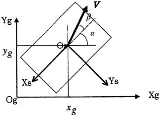
Fig. 1 Global and Ship Coordinate Systems
When (Fxg, Fyg, 0) and Mz are the total forces acting on the ship and the consequent moment about the vertical (Zg) axis, respectively, the equations of the planar motion of the ship in Σg are
(1)
(2)
(3)
where α is the heading angle between the positive Xg and the negative Xs axes, m the mass and Iz the moment of inertia of the ship. The time-integration of ![]() and
and ![]() gives the translational and the angular velocities,
gives the translational and the angular velocities, ![]()
![]() and
and ![]() respectively. Moreover, the same holds for the position (xg, yg, 0) in Σg and the heading angle α. The translational velocity (Vxs, Vys, 0) and the acceleration in
respectively. Moreover, the same holds for the position (xg, yg, 0) in Σg and the heading angle α. The translational velocity (Vxs, Vys, 0) and the acceleration in ![]() Σs are obtained by the transformation of coordinate by using α, i.e. just a rotation in this case. The angle β in Fig. 1 is the drift angle formed by the negative Xs and the translational velocity vector V=(Vxs, Vys, 0).
Σs are obtained by the transformation of coordinate by using α, i.e. just a rotation in this case. The angle β in Fig. 1 is the drift angle formed by the negative Xs and the translational velocity vector V=(Vxs, Vys, 0).
NS SOLVER
Our NS solver is called WISDAM5, which has been successfully used for the flow simulation about ships2,3,4,5) dealing with wave-making, viscous boundary layer, turbulence, etc. The method adopts the staggered allocation of pressure and velocity components in Cartesian coordinates with MAC-type algorithm for incompressibility, finite-volume formulation in a curvilinear body-fitted structured grid system, a moving free-surface-fitted grid system2) or the marker density function3) for the treatment of free surface and a combination of a Smagorinsky-type subgrid scale and a Boldwin-Lomax turbulence models4). The propeller action in the form of a body-force was incorporated into the method for the simulations of a self-propelled ship in steady straight course4). As mentioned above, we focus only on VLCCs in this study, so that the Froude number is low and double- model flow assumption may be acceptable. Accordingly, the free-surface algorithm is not activated. See the references about each computational procedure for more details. In this study, we have provided the WISDAM5 with some modifications for motion simulations, which are described in the following sections.
INERTIA FORCES IN NS EQUATION
Since a coordinate system is fixed to a ship, inertia forces are incorporated into the NS equation as body forces in Σs:
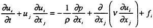
(4)
where fi is the inertia force caused by the
transformation of coordinate and is given by
(5)
where Ω is the angular velocity vector (0,0,ω) and v the flow velocity vector (us, vs, 0) and r the position vector (xs, ys, 0) in Σs. The terms in the RHS of Equation (5) indicate the Coriolis force, the centrifugal force and the unsteady forces due to angular and translational accelerations. Considering only planar motion, Equation (5) is simplified as follows:
(6)
(7)
(8)
BOUNDARY CONDITIONS
The boundary conditions for the NS solver are transient because the computational region is fixed to an arbitrarily moving ship. At the inflow, let the position vector on the boundary r0, the velocity is given by
(9)
In the case of planar motion, Equation 9 becomes as follows:
(10)
(11)
(12)
For velocity, the other conditions are the same as those of steady state simulations, i.e. no-slip on the body and zero-normal-gradient Neumann condition at the outflow. Since double model flow is assumed, symmetric condition is imposed on the still water plane.
The Neumann-type pressure condition on the body boundary has to be
(13)
which differs from steady state simulations. The others are a Dirichlet condition (p=0) at the inflow and a zero-gradient Neumann at the outflow and on the still water plane.
MATHEMATICAL MODEL FOR RUDDER, PROPELLER AND THEIR INTERACTION WITH HULL
We have chosen the so-called MMG model9) as a mathematical model, where the forces of a rudder and a propeller are represented as point-wise loads at their positions, respectively, including their interactions with a hull. They are schematically drawn in Fig. 2.
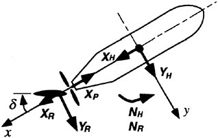
Fig. 2 Schematic of Forces and Moments Acting on a Ship
The forces and moment of a rudder are calculated by the following equations9).
(14)
(15)
(16)
where aH and xH are the interaction coefficients between the rudder and the hull, xR the nondimensional position of the rudder, δ the rudder angle and (1−tR) the thrust reduction coefficient due to the rudder. FN is the hydrodynamic normal force of the rudder usually modelled by
(17)
where AR is the area and Λ the aspect ratio of the rudder. UR and αR are the flow speed at the rudder position and the effective rudder angle:
(18)
(19)
The MMG model proposed the following form of the effective velocity at the rudder position, uR and vR,
considering the effects of the propeller9).
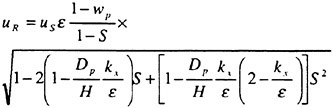
(20)
(21)
where Dp is the diameter of the propeller, Η the height of the rudder, kx the propeller acceleration ratio, γR the proportinal coefficient for the lateral component of the effective flow velocity at the rudder and lR the nondimensional lever for the rudder. The experiments indicated that γR is almost constant when the propeller is not in action but, otherwise, vR is nonlinear function of (vS+lRLPPω)9). In this study, we assume that γR is constant just for simplicity. The propeller slip ratio, S, and the ratio between the effective wake coefficients of the rudder and the propeller, ε, are given by
(22)
(23)
where n is the revolution per second and Ρ the pitch of the propeller. Several functions for (1−wP) based on (1−wP0), the wake coefficient in straight course, are suggested in the MMG model but none of them was successful under the conditon of large rudder angle9). For simplicity, we use (1−wP0) in place of (1−wP) in this study as long as the rudder angle is not very large.
In this study, thrust is a point-wise load at propeller position simply given by the simulated negative resistance to a ship in straight course as is given by
(24)
Therefore, the thrust reduction coefficient (1−tP), which is not explicit in Equation (24), is also regarded as constant during the ship motion without excessive rudder angle.
It should be noted that there are four kinds of parameters in the MMG model in the present method, i.e. the given dimensions (xR, AR, Λ, Dp, Η, Ρ), the given manoeuvring parameters (δ, n), the values empirically obtained in advance (aH, xH, (1−tR), (1−wP0), k1, ε, γR, lR) and the transient results of the NS and the motion equations (us, vS, ω).
COMBINATION OF EQATION OF MOTION AND NS SOLVER
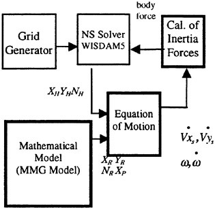
Fig. 3 Flow Chart
Fig. 3 shows the flow chart of the present simulation method. Firstly, a grid system is generated about a ship by a grid generator and is transported to our NS solver, WISDAM5. Then the steady-state solution of a ship in straight course is solved as the initial state for manoeuvring motion simulations. At this stage, thrust which will be used invariably throughout the simulation is obtained by Equation (24). Here one gives the steerage of desired ship motion. In the MMG model described above, the forces and the moments of a rudder and a propeller are calculated considering their interactions with a hull. Since WISDAM5 solves the unsteady flow about the ship time-evolutionarily, at every time step it provides the equations of motion with the hydrodynamic forces acting on the hull. Then the equations of motion are solved and the resultant translational and the angular velocities and accelerations are used for the calculation of the inertia forces, which are incorporated into the NS equation as body forces. This procedure except the grid generation is iterated at every time step. The WISDAM5 adopted explicit time-integration and, therefore, time increment is thought to be small enough to express the ship motion.
SIMULATION OF DRIFT FLOW
Before simulating the manoeuvring motion of ships, we solve drift flows in order to validate our NS solver WISDAM5. It can be said that the sufficient degree of accuracy of the drift flow simulation is a necessary condition for the success of the following Z-manoeuvring motion simulations. Recently, similar simulations of drift flow were done by Ohmori et al.5) using WISDAM5 with a moving grid system. In their method, when a ship changes its heading angle from straight to drift in the fixed computational domain, the grid system fitted to the ship has to move and alter its shape. This may limit the maximum drift angle because of the distortion of grids. Here we attempt the similar simulations by using the fixed grid system fitted to a ship.
Table 1 Principal Dimensions
|
Particulars |
Model-A |
Model-B |
|
Lpp (m) |
3.50 |
|
|
B (m) |
0.634 |
|
|
D (m) |
0.328 |
|
|
draft (m) |
0.211 |
|
|
Cb |
0.802 |
|
|
Cp |
0.806 |
|
|
Cpa |
0.7504 |
0.7557 |
|
Icb |
−2.450 |
−2.610 |
The Reynolds number (Re) of the simulation is 1.0× 10⁶, which is smaller than that of the model test (2.8 ×10⁶), because the turbulence model used in the WISDAM5 has been tuned to match forces and wake velocity distribution with those of measurements for this Re and the given grid spacing. In terms of the forces related to the planar motion of ships such as lateral force and yawing moment are not thought to be very sensitive to Re as long as the flow is turbulent and as the simulation Re has the same order of magnitude as that of the model test. Using the steady-state flow result in straight course as an initial state, a ship starts drifting at the nondimensional time (t) of 0 with keeping the translational velocity constant and reaches the target drift angle at t=0.5. The simulation lasts until the flow reaches the steady state (t>2).
We have picked two VLCCs (Model-Α and -B) with the same principal dimensions and different aft-part frame lines: one is so-called V-shaped and the other is U. The principle dimensions of these models are listed in Table 1. The drift angle is set to 9 degree. The speed of the models is 0.807 m/sec corresponding to 15 knot for the 320 m long ships. We have the model tests results under these conditions, where the motion of any degree of freedom is prohibited.
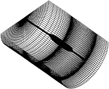
Fig. 4 Grid System for Ship Motion Simulation
As shown in Fig. 4, the computational region is half-pipe-shaped of the longitudinal length of 2.5 (−1.0 to 1.5 from the midship) and the radius of 1.0 nondimensionalised by Lpp. The number of grid points are 190,991 (101×31×61 in the longitudinal, the radial and the girth directions, respectively). The nondimensionalised minimum grid spaces in the radial direction are 1.0×10³ at FP, 0.1×10³ at midship and 0.4×10³ at AP.
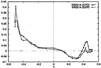
Fig. 5(a) Longitudinal Distribution of Lateral Force of Model-A
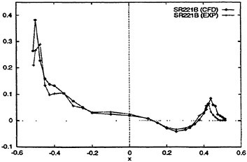
Fig. 5(b) Model-B
The comparison of the longitudinal distribution of lateral force between the simulations and the experiments of Model-Α and -B is shown in Fig. 5(a) and (b), respectively. Although the tendency of the simulated force profile agrees very well to those of the experiments, small discrepancies are observed near FP and AP in both figures, especially near AP of Model-Α, where the recovery of lateral force to the positive is larger than that of the experiment. The difference near FP may be due to the effect of bow wave which is excluded in the simulations. Fig. 6(a) and (b) indicate the contour map of pressure in the transverse plane at the position of 0.45. The pressure is nondimensionalised by ρV02 where V0 is the ship speed in straight course. Solid and dashed lines indicate the positive and the negative pressure, respectively, the interval of which is 0.02. A negative pressure zone can be seen in each figure, which corresponds to separated streamwise vortices in the wake of drift flow. It is noted that the position and the intensity of these simulated vortices affect the lateral force near AP to the significant extent.
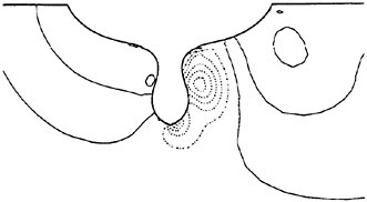
Fig. 6(a) Contour map of Simulated Pressure at x=0.45. Model-A
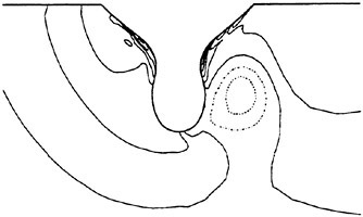
Fig. 6(b) Model-B
Fig. 7(a) and (b) show the time history of the total lateral force and the yawing moment of Model-A and -B, respectively, obtained both by the simulations and the experiments. Henceforth, forces and moment are nondimensionalised by ![]() and
and ![]() respectively. The Froude number of the experiments is 0.074 in order to make wave effects as small as possible. The simulated lateral force and the yawing moment for both models are in considerably good agreement with those of the experiments. Therefore, it can be said that the present NS solver performs very well in the drift flow and that the success in these simulations satisfies a necessary condition for its applicability to motion simulations.
respectively. The Froude number of the experiments is 0.074 in order to make wave effects as small as possible. The simulated lateral force and the yawing moment for both models are in considerably good agreement with those of the experiments. Therefore, it can be said that the present NS solver performs very well in the drift flow and that the success in these simulations satisfies a necessary condition for its applicability to motion simulations.
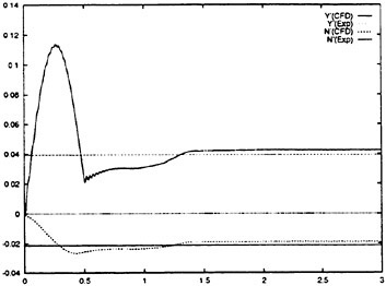
Fig. 7(a) Time History of Total Lateral Force and Yawing Moment of Model-A
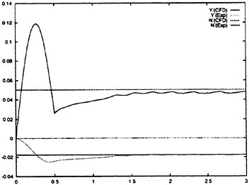
Fig. 7(b) Model-B
SIMULATION OF Ζ MANOEUVRE
Using the same grid systems as those used in the drift simulation for Model-Α and -B, respectively, we apply the present method to the simulation of 10-degree Z-manoeuvring motion. Empirical parameters in the MMG model are set to those obtained by the model tests and rudder and propeller dimensions are also those used in the tests shown in Table 2.
Table 2 Dimensions of Rudder and Propeller
|
Dimensions |
Values |
|
|
Rudder |
Area (m2) |
0.011455 |
|
Height (m) |
0.1372 |
|
|
Aspect ratio |
1.653 |
|
|
Propeller |
Diameter (m) |
0.1028 |
|
Pitch (m) |
0.0645 |
|
The position of the centre of gravity is −0.03 from the midship and the inertia radius is 0.24 for both models as set in the model test. The speed of steering is given by a constant value of 22.2 degree/sec. The Reynolds number (Re) of the simulation is 1.0×10⁶. The steady-state flow result in straight course is again used as the initial state of the Z-manoeuvring motion simulation. Firstly, the rudder starts moving at the given constant speed until its angle becomes 10 degree. Then the ship gradually starts yawing. As soon as the heading of the ship becomes 10 degree, the counter-steer is commanded to set the rudder angle to −10 degree. After the overshoot of the heading, the ship turns towards the extension of the initial heading direction. The same helm is made when the heading becomes −10 degree and, consequently, the ship is manoeuvred in a zigzag curve.
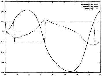
Fig. 9(a) Time History of Calculated Heading, Rudder and Drift Angles of Model-A
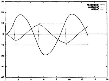
Fig. 9(b) Model-B
Fig. 9(a) and (b) show the time history of the simulated heading, rudder and drift angles of Model-A and -B, respectively. The horizontal axis indicates the time nondimensionalised by Lpp/V0: 1.0 corresponds to the real time of 4.34sec. These angles obtained by the experiments for Model-Α and -B are also shown in Fig. 10(a) and (b), respectively. The simulated results clearly indicate the typical characteristics of manoeuvrability due to frame lines in the aft part as well as the measurements, i.e. V-shaped Model-Α responds slowly to steering and, on the contrary, U-shaped Model-B makes quick response. Although the simulated timings when the heading angle reaches the extrema are about 10% earlier than those of the experiment for Model-A, the values of the extrema are in good agreement with those of the measurement. In the case of Model-B, such timings are much earlier, say 20%, and the extrema are in moderate agreement with those of the experiment. The simulated drift angles are a little larger than those of the experiments for the both models.
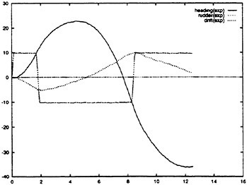
Fig. 10(a) Time History of Measured Heading, Rudder and Drift Angles of Model-A
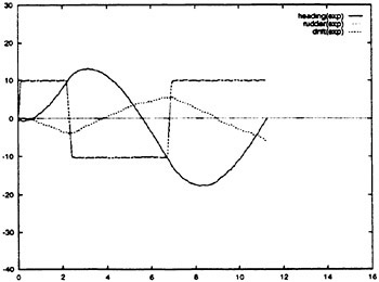
Fig. 10(b) Model-B
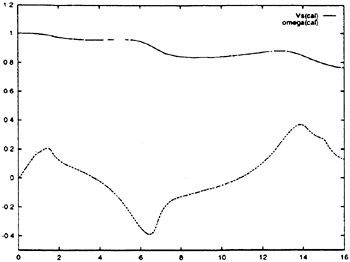
Fig. 11(a) Time History of Calculated Ship Speed and Yaw Rate of Model-A
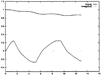
Fig. 11(b) Model-B
Fig. 11(a) and (b) indicate the time history of the simulated speed and yaw rate of the models A and B, respectively. These velocities obtained by measurements for the two models are in Fig. 12(a) and (b), respectively. In these figures, the yaw rate is stated in radian per nondimensional time of 1.0. Thrust in the simulations is simply given by the negative resistance of a ship in straight course. Nevertheless, the decrease tendency of ship speed in Figure 11 agrees well with that of the measurements, except for the difference in time axis. Similarly, the simulated tendency of the yaw rate is in good agreement, though its values are larger in the simulations than those in the experiments for the both models. This large values, especially for Model-B, correspond to the large heading angles shown in Fig. 9(b).
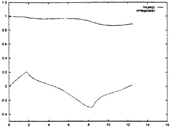
Fig. 12(a) Time History of Measured Ship Speed and Yaw Rate of Model-A
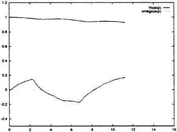
Fig. 12(b) Model-B
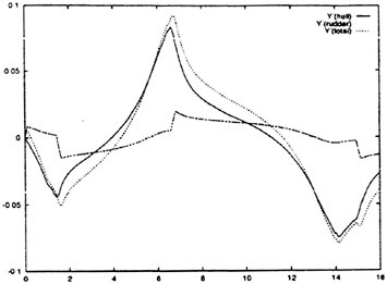
Fig. 13(a) Time History of Calculated Lateral Force of Model-A
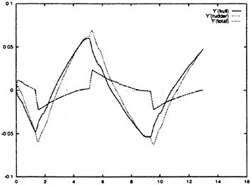
Fig. 13(b) Model-B
Fig. 13(a) and (b) indicate the time history of the simulated total lateral force and its components, i.e. the one acting on the hulls and the one calculated by the MMG model at the rudder position, of the two models, respectively. The similar components of the simulated yawing moment and their total are given in Fig. 14(a) and (b). It is observed that the forces of the hulls are dominant for the both models. On the other hand, the moments of the hulls are almost matched with those of the MMG model, especially in the case of Model-Α. This means that steer does not work so well for Model-Α, hence, the worse manoeuvrability compared with Model-B.
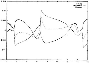
Fig. 14(a) Time History of Calculated Yawing Moment of Model-A
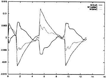
Fig. 14(b) Model-B
The simulated flow fields around both two models during Z-manoeuvring motion are shown in Fig. 15(a) and Fig. 16(a), respectively. Both figures were output at the end of computation, i.e. t=16 for Fig. 15(a) and t=13 for Fig. 16(a). Similar figures obtained by the above-mentioned drift flow simulations are also shown in Fig. 15(b) and Fig. 16(b), respectively, for comparison. Velocity vectors and pressure contours with intervals of 0.02 are drawn on the 10th and the 42nd plane roughly normal to the girth direction. Because there are 30 planes in the girth direction for the half side, they are located about one third of a right angle from the still water plane. The remarkable difference between Fig. 15(a) and (b) is the values of pressure. This is because of the reduction of ship speed shown in Fig. 11(a), where the ship speed becomes about 0.8 at t=16. However, the contours of pressure have similarity in these two figures. This can be explained by the fact that the drift angle of 9.85 degree at t=16 shown in Fig. 9(a) is close to the angle set in the steady drift flow simulation and that the yaw rate is trivial at this instance as shown in Fig. 11(a), so this temporary flow field resembles that of the drift flow. It can be also said that the unsteady force caused by ![]() does not have significant effects even though the yaw rate is in the middle of gradient as shown in Fig. 11(a).
does not have significant effects even though the yaw rate is in the middle of gradient as shown in Fig. 11(a).
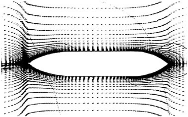
Fig. 15(a) Calculated Velocity Vectors and Contour Map of Pressure at t=16 in Z-Manoeuvring Motion of Model-A
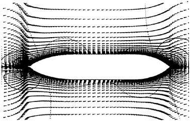
Fig. 15(b) in Drift Flow of Model-A
On the other hand, contours of pressure in Fig. 16(a) is quite different from those in Fig. 16(b). For instance, positive pressure near the bow in Fig. 16(a) seems symmetric unlike that in Fig. 16(b) and the negative pressure region starting from the stern is leant more than that in Fig. 16(b). The latter cannot be explained by the fact that the drift angle at this instance of Fig. 16(a) is 6.80 degree, which is smaller than that of Fig. 16(b). This can be attributed to the large yaw rate at t=13 as shown in Fig. 11(b), for the centrifugal force bends the flow direction throughout the ship length as shown by velocity vectors in Fig. 16(a).
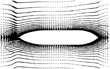
Fig. 16(a) Calculated Velocity Vectors and Contour Map of Pressure at t=13 in Z-Manoeuvring Motion of Model-B
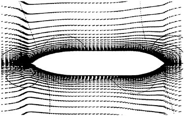
Fig. 16(b) in Drift Flow of Model-B
CONCLUSIONS
A numerical simulation method has been developed for solving the manoeuvring motion of blunt ships by coupling the equations of motion of ships and the NS equations. Our target is VLCCs so that the only planar motion in the horizontal plane is considered and the effects of wave are thought to be negligible because its Froude number is very low. The hydrodynamic forces acting on the hull of a ship are obtained by our NS solver WISDAM5 and the forces and the moments of a rudder and a propeller and their interactions with the hull are computed by a mathematical model called MMG. Since a coordinate system is fixed to an arbitrarily moving ship, inertia forces are incorporated into the NS equation as body forces.
In order to confirm the accuracy of our NS solver, we compared simulated results with those of measurements for the 9-degree drift flow about two VLCC models with the same principal dimensions and different frame lines in the aft part: one is so-called V-shaped and the other is U. It was elucidated that the low pressure near AP due to the streamwise vortices separated from the hull plays a significant role to affect the total lateral force and, especially, the yawing moment. The simulation performed very well to predict the lateral force and the yawing moment. It
is regarded that this fact satisfies a necessary condition for applying the present method to motion simulations.
Then we moved to the 10-degree Z-manoeuvring motion of the two models. The results of the simulations are in qualitatively good and quantitatively reasonable agreement with those of the experiments and represent sufficiently the typical difference of manoeuvrability between the models, i.e. Model-Α with V-shaped frame lines shows directional instability with the large overshoots of heading angle and, on the contrary, Model-B with U-shaped frame lines responds quickly to rudder movement. More test simulations for VLCCs will be able to accumulate the reliability of this method in predicting the manoeuvrability of newly designed ships.
ACKNOWLEDGEMENT
This study is conducted as part of SR229 project sponsored by the Shipbuilding Research Association of Japan. The authors thank the LINEC Research Group for their instructive comments. Particularly, we would appreciate the offer of grid systems and experimental data from Dr. T.Ohmori of IHI, Mr. M.Takai of SHI and the SR221 project team.
REFERENCES
1. Hearn, G., Clarke, D., Chan, H., Incecik, A. and Varyani, K., “The Influence of Vorticity upon Estimation of Manoeuvring Derivatives”, Proceedings of the 20th Symposium on Naval Hydrodynamics, National Research Council, Jun. 1994, pp. 669–681.
2. Miyata, H., Zhu, M. and Watanabe, O., “Numerical Study on a Viscous Flow with Free-Surface Waves about a Ship in Steady Straight Course by a Finite-Volume Method”, Journal of Ship Research, Vol. 36, No. 4, 1992, pp. 332–345.
3. Kanai, A. and Miyata, H., “Numerical Analysis of Structure of Free-Surface Shock Wave About a Wedge Model”, Journal of Ship Research, Vol. 40, No. 4, 1996, pp. 278–287.
4. Kawamura, T., Mashimo, K., Masuda, S., Kimura, K., Mitsutake, H. and Ando, J., “Finite-Volume Simulation of self-propelled Tanker Models”, Proceedings of the 3rd Korea-Japan Joint Workshop on Ship and Marine Hydrodynamics, Society of Naval Architects of Korea and Society of Naval Architects of Japan, 1996, pp. 105–114.
5. Ohmori, T., Fujino, M. and Miyata, H, “A Study on Flow Field around Full Ship Forms in Maneuvering Motion”, Journal of Marine Science and Technology, to appear.
6. Davoudzadeh, F., Taylor, L.K., Zlerke, W.C., Dreyer, J.J., McDonald, H. and Whitfield, D.L., “Coupled Navier-Stokes and Equations of Motion Simulation of Submarine Maneuvers Including Crashback”, Proceedings of Fluids Engineering Division Summer Meeting, ASME, 1997, FEDSM97–3129, pp. 1–8.
7. Dreyer, J.J., Taylor, L.K., Zlerke, W.C. and Davoudzadeh, F., “A First-Principal Approach to the Numerical Prediction of the Maneuvering Characteristics of Submerged Bodies”, Proceedings of Fluids Engineering Division Summer Meeting, ASME, 1997, FEDSM97–3130, pp. 1–8.
8. Takada, N., “3D Motion Simulation of Advancing Bodies with Mobile Wings by CFD”, Master Thesis, University of Tokyo, Mar. 1998 (in Japanese).
9. Kose, K., Yoshimura, Y. and Hamamoto, T., “Mathematical Model Used for Prediction of Manoeuvrability and Model Test”, Bulletin of the Society of Naval Architects of Japan, Society of Naval Architects of Japan, Vol. 668, 1985, pp. 63–75 (in Japanese).
DISCUSSION
S.Yang
Korea Research Institute of Ships and Ocean Engineering, Korea
I would first like to thank the authors for presenting an interesting paper. This paper provides a valuable step toward the direct simulation of ship maneuvering motions by CFD. Although they use an empirical model for the rudder and propeller, their results are very encouraging.
My first question is concerned with the treatment of boundary conditions. The paper states that incoming flow condition is given at the inflow boundary and a zero gradient boundary condition is applied at the outflow boundary. But it’s not clear how you divide the outer boundary into the inflow boundary and outflow boundary when incoming flow is changing continuously. You seem not to be able to take in enough computational domain. Do you think that your computational domain is sufficiently wide to remove any reflections from the outflow boundary?
When we predict maneuvering motions by a mathematical model, MMG model for example, the inflow angle into the rudder (or VR in Equation (21)) is as important as the forces acting on the ship hull. So, it would be very interesting to see how much CFD can predict this property well. Could you show me your computed velocities at the rudder compared with experimental data?
AUTHORS’ REPLY
We would like to thank Dr. S.I.Yang for his discussion. His first question is about boundary conditions and the size of computational domain. Figure 4 denotes the present computational domain around a ship. The half circle locating at the right-down in Fig. 4 is the inflow boundary on which a Dirichlet condition for velocity is imposed. The other half circle at the left-top and the side wall of the half pipe are the outer boundaries with the zero-gradient condition for velocity. It might be noticed that this is normally recognized as a set of boundary conditions for the flow in straight course. Here the same is applied to drift flow or Ζ maneuvering motion simulations. When drift angle is small, say 10 degrees like the present simulations, we have experienced no problem for computation with this domain and this set of conditions. If the angle is large, it might be necessary to consider widening the domain and dividing the side into two different kinds of boundaries. In this case, the inflow may be determined by the sign of the mass flux through each cell-face of the side boundary. If free-surface waves are taken into account, the domain ought also to be enlarged for damping the waves and avoiding their unphysical reflections from the boundaries.
Secondly, the discusser asks for the comparison of the velocity at rudder position between CFD and measurements. As he mentioned, the value of vR is particularly important to demonstrate the MMG model because it determines the attack angle of the rudder as shown in Eq. (17). Here the method to obtain vR is the empirical way shown by Eq. (21). Hence, the prediction of vR totaly depends on the form of Eq. (21) and hardly on the velocity at rudder position obtained by CFD. Just like experiments, CFD only provides Eq. (21) with balk values such as vS and ω, the lateral component of ship speed and the angular velocity of a ship in the global coordinates. Therefore, the comparison of velocity requested by the discusser may not satisfy him in this context.
However, such comparison is very important for the validation of CFD. Figure 17 denotes velocity vectors and the nominal wake contours by CFD and measurement, respectively, on the section plane at A.P. for Model A. The condition of CFD and measurement is for 9-degree steady drift flow without rudder and propeller. Similarly, those for Model Β are shown in Fig. 18. It is fair to say that CFD predicts the velocity field very well.
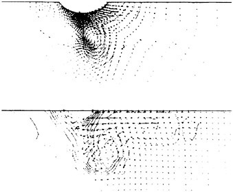
Fig. 17 Velocity vectors and nominal wake contours at x=0.5 in 9-degree drift flow for Model-A. Contour interval is 0.1. Simulated (upper) and measured (lower).
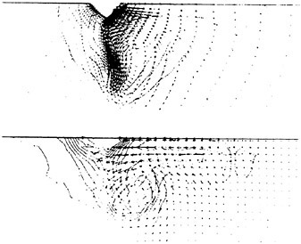
Fig. 18 Velocity vectors and nominal wake contours at x=0.5 in 9-degree drift flow for Model-B. Contour interval is 0.1. Simulated (upper) and measured (lower).
DISCUSSION
D.Liut
Virginia Polytechnic Institute and State University, USA
What sort of solver method was used to solve for the differential equations of motion?
AUTHORS’ REPLY
The equations of motion of a ship shown in Eqs. (1) to (3) are not solved by any special method. Once accelerations are obtained by solving them, velocities and positions are calculated by time-integration stated below.
(25)
(26)
DISCUSSION
G.Hearn
University of Newcastle Upon Tyne, United Kingdom
Thank you for your very interesting paper. Some years ago in a discussion with van Hooft at MARIN, in Holland, van Hooft suggested that forces and moments rather than hydrodynamic derivatives should be used in analyzing the maneuvering ship. In this paper you show in Figure 6 the existence of the vortex for both models A and B. In earlier comments made by myself during the conference, I have indicated the importance of the presence of the vortex upon the hydrodynamic forces. Additionally, I would expect that your methodology would be capable of demonstrating a pair of vortices which move relative to the hull as the drift angle increases, up to the point where the drift angle is sufficiently large to produce vortices on one side of the hull. In other words, demonstrate the physical properties expected of a good mathematical model. Have you undertaken such an exercise? Could you provide some intermediate results?
AUTHORS’ REPLY
We appreciate the discusser’s instructive comment and question. Figures 19(a) to (c) denote the distribution of helicity (the scalar product of velocity and vorticity vectors) on the section plane of x=0.45 at the moment when the drift angle becomes 0, 3 and 5 degrees, respectively, at the beginning of Z maneuvering motion for Model B. They correspond to the nondimensional time of 0 to 2, approximately, in Fig. 9(b).
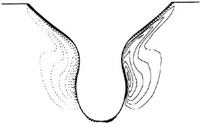
Fig. 19(a) Contour map of simulated helicity at x=0.45 during Ζ manoeuvring motion. Contour interval is 10.0. Solid contours indicate anticlockwise rotation. Model-B β=0°
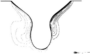
Fig. 19(b) β=3°
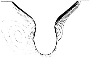
Fig. 19(c) β=5°
In Fig. 19(a), there are a pair of symmetric and remarkable vortices in the starboard and the portside of Model-B. Each one is probably the mixture of a so-called bilge vortex and the one generated in the boundary layer of upward flow due to the longitudinal change of hull shape. Moreover, there is a very thin counter-rotating vortex along the side wall near the water plane in each side, which wedges between the wall and the upper part of the upward-boundary-layer vortex. This may be resulted from the boundary layer of downward. In Fig. 19(b) and (c), the windward mixed-bilge vortex shrinks. On the contrary, the leeward one becomes larger and has two humps in Fig. 19(c). As is mentioned above, the hump near the wall is originated from upward boundary layer and the other corresponds to the bilge vortex separated far from the hull by cross flow.
The transient behavior of streamwise vortices ought to be paid special attention to, because it is thought that such dynamics must affect the unsteadiness of forces acting on the hull. Such vortex dynamics will possibly be a new target of CFD motion simulations in the near future.
Inviscid Calculations of Ship Wave Making—Capabilities, Limitations, and Prospects
H.Raven (Maritime Research Institute, The Netherlands)
1 Introduction
The prediction of the wave pattern generated by a ship sailing in still water has made rapid progress during the last two decades. After extensive work on thin ship, slender body and Neumann-Kelvin theories in the fifties and sixties, the introduction of Dawson’s linearised method in 1977 started a period of renewed interest in the prediction of ship wave patterns. Dawson’s method was widely reproduced and many variations have been developed. For the first time wave resistance research thus led to a frequent use of free-surface potential flow predictions in practical ship design.
The flexibility and success of these methods, and the ever increasing computer speed, around 1986 inspired a next step: the development of methods to solve the same problem with fully nonlinear free surface boundary conditions. As it turned out, this meant another major step forward in accuracy and completeness of the predictions. After a decade of work on this class of methods, a few of them are mature and are actually being applied in practical merchant ship design.
It is these nonlinear free surface potential flow solvers that are the subject of this paper. We shall attempt to survey and illustrate what one may expect today of nonlinear inviscid methods for wave pattern calculation. This information may also put in perspective the current research emphasis on viscous flows with free surface boundary conditions, more precisely indicating to what extent viscous effects on wavemaking are significant.
A brief review of the leading methods, their similarities and main differences, is given in Section 2. It appears that almost all of these apply so-called ‘raised-singularity’ methods. Section 3 presents a theoretical analysis, which not only indicates many of the properties of such methods, but also points the way toward a novel finite difference scheme to be used in the free-surface boundary condition. This scheme apppears to eliminate most of the numerical damping.
Sections 4 and 5 address two critical issues in this class of methods: the accuracy of the wave resistance prediction, and the capability to predict the flow and free surface detachment off the stern. Recent progress and validation results for the RAPID method are discussed. Sections 6 and 7 then summarise current capabilities and shortcomings, describe what problems are still unsolved from the practical or fundamental point of view, and give a view on the way ahead.
2 Nonlinear steady ship wave prediction methods
First we briefly consider the main existing nonlinear free surface potential flow solvers. We shall limit ourselves to codes that can be and are regularly being applied for predicting the steady wave pattern of practical ships. While several new developments have been published over the years, most of these seem not to have been pursued or have just been demonstrated with cases in the Wigley hull/Series 60 category, and will be disregarded here. Moreover, we shall leave out of account the variety of existing linearised methods. With those limitations, only a few methods remain. The methods mostly considered in this section are SHALLO, RAPID, and SHIPFLOW.
SHALLO was developed at Institut für Schiffbau in Hamburg by Jensen and Söding, starting around 1986. [1, 2]. This method contains several original ideas, some of which have found widespread adoption. The code is in frequent use at HSVA. No validations or extensions seem to have been published recently.
RAPID [3, 4] was developed by the present author at MARIN, starting in 1990. Since 1994 it is being applied on a large scale at MARIN in practical ship design projects and research, now at a rate of several hundreds of calculations per year. In addition, it has
been installed at 5 shipyards and one university.
SHIPFLOW, or more specifically its module XPAN, originally was developed by Ni at Chalmers University [5], then reprogrammed by Kim [6], then revised by Janson [7], in cooperation with the Flowtech company. While the code has had several versions, its present basic form is quite similar to RAPID. Some 25 external installations at yards, universities and consultants exist.
There is a more recent code VSAERO/FSWAVE (1996), started again at IfS in Hamburg by Hughes, now being used by AMI [8]. It has adopted several features of the previous codes, married with the basic VSAERO methodology. Little has been published on its properties and accuracy.
The code SPLASH, developed by Rosen, since recently has a nonlinear version [9] which is rather unlike the previous ones. The paper on the nonlinear version gives no information on grid dependence, convergence and accuracy, but suggests that the nonlinear code is not yet mature enough for large-scale application. The method was primarily set up for sailing yachts, and these are almost the only applications shown.
The method once published by Daube [10] recently turned up again, but I am not aware of a more recent publication on the new code.
Finally, we probably are overlooking or disregarding some less known or unpublished but possibly qualifying codes; hopefully this will not harm the validity of the general picture.
2.1 Basic formulation
All of these methods solve the problem of a steady potential flow with free surface around a ship hull. At the actual free surface, the boundary conditions of constant (atmospheric) pressure and zero normal velocity are imposed. The free surface domain included is of finite extent, and outside its truncation boundary the fluid domain is open. The potential flow is determined from a boundary integral equation which involves the wetted hull surface and a boundary connected with the free surface.
In addition to the boundary conditions mentioned above, a ‘radiation condition’ is to be satisfied, which excludes the occurrence of waves upstream of the ship. We come back to this in Section 2.4 below.
2.2 Iteration
The nonlinearity of the free surface boundary conditions (FSBC), and the necessity to impose these on the initially unknown wave surface, require either time stepping or iteration. The former means an initial value approach, starting from any initial condition and time stepping until a steady result has been obtained. This procedure has a natural and well-proven formulation, but it may settle to steady state only slowly, e.g. due to the slow decay of oscillations related to the ![]() singularity.
singularity.
All methods mentioned above apply the other alternative and solve the steady form of the problem by iteration. As it turns out this is far more efficient. On the other hand, the formulation of the FSBC and the wave height updates is less obvious than in initial-value methods. One might think of imposing the kinematic condition in each iteration, and using the dynamic condition to update the wave surface, or the other way round. However, this will fail or be inefficient. Instead, all methods considered apply a combined condition, which is obtained by writing the kinematic FSBC in terms of the wave height; and substituting this by the expression obtained from the dynamic FSBC:
(1)
(The y-coordinate is vertically upward here, and ![]() is the potential including that of the undisturbed inflow). This combined FSBC is subsequently linearised in perturbations of the solution of the previous iteration. This linearised combined FSBC is basically Kelvin-like, and even more resembles Dawson’s linearised FSBC. Thus it includes already much of the physics; e.g. the first iteration will produce a Neumann-Kelvin solution which, while not perfect, is already a physically quite plausible initial solution. This property makes the combined FSBC the best choice for a condition to be imposed in each iteration in a nonlinear procedure.
is the potential including that of the undisturbed inflow). This combined FSBC is subsequently linearised in perturbations of the solution of the previous iteration. This linearised combined FSBC is basically Kelvin-like, and even more resembles Dawson’s linearised FSBC. Thus it includes already much of the physics; e.g. the first iteration will produce a Neumann-Kelvin solution which, while not perfect, is already a physically quite plausible initial solution. This property makes the combined FSBC the best choice for a condition to be imposed in each iteration in a nonlinear procedure.
The iterative procedure thus requires solving the Laplace problem for the potential under the last guess of the free surface, subject to the linearised combined FSBC on that surface; from the new solution, updating the wave surface and free surface velocity field; and starting the next iteration. To update the wave surface between iterations, all methods then use the dynamic FSBC.
While the methods discussed have the same basic procedure, there are some differences in the form of the FSBC in detail. After convergence these differences vanish; but they may affect the convergence rate. E.g.: - some include the ‘transfer terms’ obtained by Taylor expanding the FSBC from the old to the new wave surface; a step that is deliberately avoided in RAPID because these terms introduce higher derivatives of the potential that are liable to be oscillatory or poorly approximated. - After the wave surface update, the next iteration requires a new guess of the velocity field at the new wave surface in order to set up the new linearised FSBC. Most methods simply take the free surface velocities on the
old wave surface for this, which in principle is inconsistent with including the transfer terms. As opposed to this, RAPID recomputes the free surface velocity field in the new points, which requires an additional matrix-vector multiplication.
It turns out, however, that these details are rather unimportant for the convergence behaviour, and much less dominant than e.g. the panel distribution and collocation point positions.
2.3 Convergence
In the first years of these developments, the convergence of this iterative procedure still was a key point. While standard test cases as Wigley hulls and Series 60 converged well, fuller ship forms or more severe nonlinearities presented many problems. In a ‘workshop’ organised between the developers of SHALLO, SHIPFLOW and RAPID in 1992 (unpublished) we considered a Series 60 Cb=0.60 hull with various free surface panellings, in order to assess the grid dependence of the solutions. It appeared that not all methods were able to handle all of these grids. To some extent, the stability of the various methods appeared to be related with the care given to numerical details. The nonlinear inviscid problem is unforgiving with regard to locally introduced errors or inherent instabilities.
Nowadays these difficulties largely have been overcome for the major codes, which can deal with a wide variety of practical cases without convergence difficulties and without resorting to any free surface smoothing procedure. In Section 6.2 some limitations will be mentioned. The number of iterations needed seems to be rather similar for most methods, and lies between 5 and 20 for usual cases. It is important in this regard that the convergence is not determined from simple inspection of the hull wave profile, as was occasionally done initially, but from a rigorous set of termination criteria. A maximum norm for the residues in the kinematic and dynamic FSBC forms such a set.
2.4 Implementation of the radiation condition
A specific property of the steady formulation is that it requires a ‘radiation condition’ that excludes waves upstream of a generating disturbance. All methods impose this condition ‘numerically’. There are two basic approaches for this. One is the use of an upwind finite difference scheme applied to the dominant terms in the combined FSBC; a method introduced by Dawson [11]. The other is a forward shift of the collocation points relative to the panels over one panel length, a method introduced in [1] and [12]. In this case there is no need to use finite differencing for any of the terms in the FSBC, if also the second derivatives of the potential are evaluated as simple sums over panel contributions. Both approaches are combined with suitable zero-perturbation conditions at the upstream edge of the free surface domain.
No difficulties with either of these basic approaches are reported. The latter method is used in SHALLO and VSAERO/FSWAVE, the former one in RAPID, SPLASH and SHIPFLOW (which exists in a version using the latter as well). Further consequences of this aspect are discussed in Section 3.
2.5 The Laplace problem
All methods mentioned are of the panel- or boundary integral class. The most striking common feature of the leading methods is the use of “raised panels” or “desingularisation” for the free surface. This means that the singularities are at a certain distance above the free surface, while evidently the collocation points (where the FSBC is satisfied) are on the free surface itself. Of the methods mentioned, only SPLASH uses panels on the wave surface itself.
More specifically, SHALLO uses point sources at a distance above the wave surface, combined with a particular treatment of the hull with panels on the hull surface itself. RAPID uses raised panels for the free surface, again with usual panels for the hull. SHIPFLOW initially had sources on the free surface, but switched to raised panels after the proven success of SHALLO and RAPID; and immediately obtained a better robustness and accuracy. VSAERO/FSWAVE is based on a Green’s identity form for the hull, but with only raised source panels for the free surface. In all methods the singularities are at around one typical panel dimension (or source spacing) above the wave surface. In most methods, they are adjusted from time to time during the iteration process in order to keep the distance more or less constant; which is important for accuracy and stability.
This application to the steady wave making of a ship to my knowledge is the only one in which the ‘desingularised’ formulations are so dominant. The question arises why this is so; and in addition, as such formulations are unusual, what precisely are their properties. This will be addressed in Section 3.
2.6 Transom sterns
A treatment of transom sterns is indispensable in a nonlinear method. The most common type of stern today is a transom at some distance above the still waterline. At speed the water surface rises to the transom edge, and
the particular type of flow occurring requires a special treatment.
The methods mentioned differ here. SHALLO and VSAERO/FSWAVE put panels on the transom, and impose a normal velocity determined such that the pressure is atmospheric at the transom edge. RAPID leaves the transom open, but imposes the transom boundary conditions by adding some strips of panels on the free surface aft of the transom. In the collocation points directly adjacent to the transom, a combination of the kinematic and dynamic condition is again imposed, but one in which the slope of the buttocks and the height and shape of the transom edge occur [13]. This takes into account the semi-singular behaviour that may occur at the transom edge, and retains the second-order accuracy. SHIPFLOW applies a similar but cruder implementation with a two-point difference scheme. Moreover, up to now SHIPFLOW could not deal with transom sterns above the still water line and simply left a triangular segment of the free surface open. This will be changed soon.
Validations of this transom modelling have only been published for RAPID [4, 14]. They indicate that it captures the principal effects, but obviously not the viscous effects. Section 5 addresses this point.
2.7 The RAPID code
Much on RAPID already has been published [3, 4, 13, 14] so some general remarks will suffice here. Main incentive to use a raised-panel form in this method was the assumed benefit for stability of keeping the free surface panels fixed for some time; and the possibility to directly compute a new free-surface velocity field from the source strengths. The advantages for robustness and accuracy were larger than anticipated. A simple accuracy analysis in [3] already indicated a much smaller numerical dispersion than with a conventional method. This stability and accuracy analysis has later been extended, and has formed an important guideline for further improvements (Section 3).
Further innovative issues related to the RAPID development are the transom flow treatment mentioned above, and the iterative matrix solver based on a pre-conditioned GMRES iteration. At MARIN the code usually runs on a CRAY C912 supercomputer, reaching Mflop rates up to 750 on a single 1 Gflop processor; an entire calculation in general takes no more than 10 minutes CPU. A typical calculation time on a SGI O2 workstation (nominal speed≈5 specfp95) is 7 minutes per iteration for 4000 panels.
The code is in continuous use at MARIN in practical hull form design, and appears to respond accurately to hull form changes, such that sensible fine-tuning of the design is warranted. New design avenues have thus been opened, specifically in bulbous bow and transom stern design.
3 Numerical dispersion, damping and stability of raised panel methods
This survey indicates a predominance of raised singularity methods for this application. The general experience is that these produce a large improvement of stability and accuracy, and the question is why. Moreover, guidance is desired to choose some of the additional parameters for these unusual methods.
To answer these questions, we shall analyse the properties theoretically, using the very useful analysis methodology developed by Nakos and Sclavounos [15]. This was already applied to raised panel methods in an incomplete form in [3], and was much extended in [4]. Later, Janson [7] extended this work by including higher-order panel methods, and methods with analytical differentiation instead of finite differencing in the FSBC. More recently, Bunnik [16] did a similar analysis for a 3D unsteady raised-panel method. Together these studies provide a sound theoretical basis permitting to understand and optimise raised panel methods. An example of the latter will be given in Section 3.5.
3.1 The analysis
Only the main line of the analysis is presented here; details can be found in [4]. The accuracy aspect typical for our problem is the representation of surface waves. The study addresses the errors in the prediction of the wave lengths (numerical dispersion) and wave amplitudes (due to numerical damping). The main error sources involved are the discretisation of the continuous free surface source distribution, and (if used) the difference scheme approximating the velocity derivatives occurring in the free surface condition. Errors due to the truncation of the free surface distribution and the discretisation of the hull source distribution are left out of account here.
While evidently the basic interest is the accuracy of the final nonlinear solution, and the stability of the solutions of all iterative steps, we restrict ourselves to a linear 2D problem to simplify the analysis. The boundary condition imposed is the Kelvin condition:
where k0=g/V2 and is the ![]() potential induced by the free surface singularities only. We have accommodated all other disturbances (e.g. a submerged body generating waves) in a right hand side supposed to be known.
potential induced by the free surface singularities only. We have accommodated all other disturbances (e.g. a submerged body generating waves) in a right hand side supposed to be known.
3.2 The continuous case
For reference we first consider a continuous source distribution with infinite extension, in a horizontal plane y=yfs above the undisturbed free surface. We represent this distribution by a Fourier series:
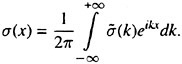
(2)
We derive the velocity components induced by σ(x) at the still water plane y=0, and substitute these in the Kelvin condition. Thus we obtain a boundary integral equation of the form:
(3)
Doing so for the Fourier modes of σ we similarly get the Fourier transformed equation:
(4)
with
(5)
The same procedure for a source distribution on the still water surface produces the same expression for ![]() except for the factor
except for the factor ![]() due to the distance of the raised source distribution from the free surface it must have a larger amplitude than if it were on the free surface itself.
due to the distance of the raised source distribution from the free surface it must have a larger amplitude than if it were on the free surface itself.
We recast this expression into one for the vertical velocity component instead of the source strength, being physically more meaningful:
(6)
with
(7)
It follows that the solution for the vertical velocity in the continuous case is:
(8)
The zero of the Fourier transform of the operator ![]() determines the wavelike behaviour of the solution far downstream; this has the wavenumber k=k0 as it should. More generally, the operator for the velocity components is of exactly the same form as for a non-raised source method. This confirms that the distance of the continuous source distribution to the water surface has no effect on the velocity field, only on the amplitude of the source distribution.
determines the wavelike behaviour of the solution far downstream; this has the wavenumber k=k0 as it should. More generally, the operator for the velocity components is of exactly the same form as for a non-raised source method. This confirms that the distance of the continuous source distribution to the water surface has no effect on the velocity field, only on the amplitude of the source distribution.
3.3 The discrete case
Much larger differences between raised and conventional panel methods appear in the discrete case. We here consider methods using raised source panels and a difference scheme for the velocity derivatives; other options will be discussed subsequently. The source distribution is discretised in constant-strength source panels of size hx located at y=yfs=αhx and centred around x=j.hx.
The collocation points are on the still water surface y=0, but may be shifted upstream relative to the panel centres over a distance γhx. This collocation point shift, a feature introduced in RAPID from the beginning, permits to optimise the properties of the method. Note that such a shift is only permitted in a raised-singularity method, as otherwise it would cause excessive numerical damping. As the shift is over a fraction of the panel length only, it serves a quite different purpose than the one-panel length shift meant for imposing the radiation condition in some methods.
Just as in the continuous case, the procedure is now to derive the velocity components induced by a source distribution, and to substitute these in the FSBC, to obtain a boundary integral equation. To study the properties of the linear operator we now introduce Discrete Fourier Transforms according to:
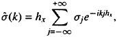
(9)
which implies an expression for the source distribution as:
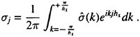
(10)
The induced velocities have the form
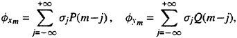
(11)
to which we can apply a discrete convolution theorem. We then find:
(12)
The factor ![]() is a shift factor to make the effect of the collocation point shift explicit.
is a shift factor to make the effect of the collocation point shift explicit.
The next step is to express ![]() in
in ![]() using the upwind difference scheme. For the Discrete Fourier Transforms this amounts to a multiplication with the DFT of the difference scheme:
using the upwind difference scheme. For the Discrete Fourier Transforms this amounts to a multiplication with the DFT of the difference scheme:
(13)
Collecting all expressions now and substituting them in the Discrete Fourier Transform of the Kelvin boundary condition produces an expression quite similar to (6) but now valid for the discrete case. Again eliminating the source strength we finally derive the expression for the vertical velocity at the free surface:
(14)
(15)
The last step is the transition from Fourier to physical space, in which use is made of the aliasing theorem and the periodicity of the operator. The expression then obtained is:
(16)
which is identical to the corresponding expression for the continuous case, (8), save for the factor ![]() replacing
replacing ![]() .
.
Therefore, for equal RHS the difference of the vertical velocity distribution in the continuous and the discrete case is entirely embodied in the difference between the Fourier transform of the continuous operator ![]() and the Discrete Fourier Transform of the operator for the discretised method,
and the Discrete Fourier Transform of the operator for the discretised method, ![]() . This difference will be cast in the same form as done in [15] and [17] to permit a direct comparison with the results given there. We define a nondimensional wave number
. This difference will be cast in the same form as done in [15] and [17] to permit a direct comparison with the results given there. We define a nondimensional wave number
which essentially is panel size divided by wave length; and the panel Froude number
The Fourier transforms of the operators then can be written as:
(17)
(18)
where
(19)
The operators relating the vertical velocity distribution on the free surface to the forcing now appear to differ by the deviation of the function Lh(s) from s. The properties of the discretised method can now be inspected by making graphs of the real and imaginary parts of Lh(s), such as Fig. 1. The diagonal line
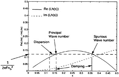
Figure 1: Interpretation of real and imaginary part of Lh(s).
Lh(s)=s is the exact solution, the continuous operator. The horizontal deviation of ![]() from the diagonal indicates the numerical dispersion. The principal far-field wave number found by the discretised method is determined by
from the diagonal indicates the numerical dispersion. The principal far-field wave number found by the discretised method is determined by ![]() as indicated by the intersection with the horizontal line. The numerical damping is proportional to
as indicated by the intersection with the horizontal line. The numerical damping is proportional to ![]() for the s-value thus found. As indicated in the figure there may be a secondary intersection. This indicates a spurious wave number that may pollute the numerical solution.
for the s-value thus found. As indicated in the figure there may be a secondary intersection. This indicates a spurious wave number that may pollute the numerical solution.
3.4 Results
Of the many conclusions that can be drawn from the analysis, the principal ones will be illustrated here. We first disregard the errors introduced by the difference scheme and just consider those due to the discretisation of the source distribution.
-
Discretising a raised source distribution in constant-strength source panels causes almost no numerical dispersion; for a non-raised method, there is a large numerical dispersion. (Fig. 2) For the raised-panel method, Re(Lh(s)) precisely follows the diagonal line up to s≈0.3, (3 panels per wavelength). For a more usual panel density of 20 per wavelength, the numerical dispersion is only 0.03% for a standard panel elevation, while a conventional method has 7.4% numerical dispersion. The figure also shows that the raised-panel method has a slight numerical damping that may affect wave components shorter than 6–7 panel lengths.
-
There is very little effect of the distance of the panels above the wave surface, α, for lower s-values (Fig. 3). A too small distance produces an earlier onset of numerical damping. The upper
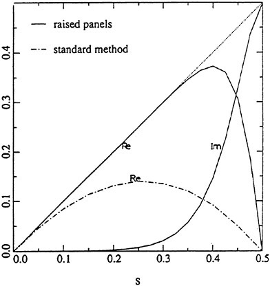
Figure 2: Lh(s) for raised-panel method and conventional method; without errors due to difference scheme. α=1.0, γ=0.25.
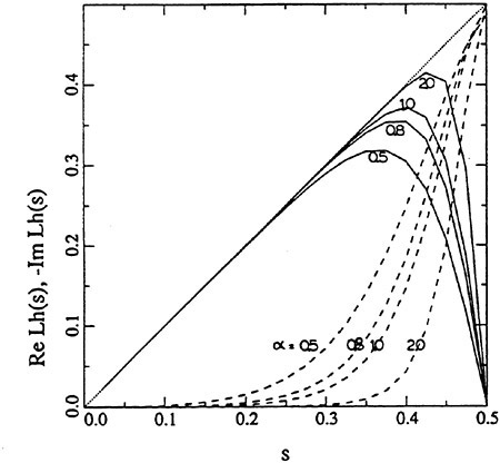
Figure 3: Effect of distance of panels above water surface for raised-panel method. γ=0.25, varying α.
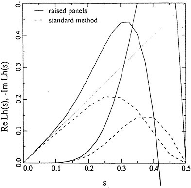
Figure 4: Lh(s) for raised-panel method and conventional method; both using Dawson’s difference scheme. α=1.0, γ=0.25.
-
limit of the panel elevation is not determined by accuracy but by robustness and by the conditioning of the set of equations.
-
The forward shift of collocation points relative to panel centres, γ, has no effect on the accuracy for s<0.2 provided a sufficient panel elevation is used; but it has a very significant effect on the numerical damping at high s-values. This will be discussed later.
The next step is to inspect the effect of the difference scheme. As ![]() has real and imaginary parts, it modifies both the dispersion and the damping. The outstanding accuracy of the raised-panel discretisation is now significantly affected.
has real and imaginary parts, it modifies both the dispersion and the damping. The outstanding accuracy of the raised-panel discretisation is now significantly affected.
-
The raised-panel method with difference scheme has a numerical dispersion of
 which produces a somewhat too large wavelength. A conventional method has a much larger numerical dispersion of
  giving a too small wavelength. (Fig. 4) For the raised-panel method the numerical dispersion at lower s-values is due to the difference scheme only; in the conventional method it is primarily due to the source discretisation and it is reduced by the difference scheme. For the raised-panel method, for s=0.05 the numerical dispersion varies between 1.0 and 1.7%, while it is 5.7% with the conventional method.
-
Note that a common panel density for RAPID is 30 panels/wavelength. In that case, even for waves diverging at an angle of 70 degrees s<0.1.
-
The raised-panel method with forward shift is stable with respect to point-to-point oscillations. The conventional method is unstable for vanishing panel size (Fig. 4). Both methods have a spurious wavenumber. However, for the conventional method this approaches s=0.5 upon panel refinement. Since the numerical damping vanishes there, point-to-point oscillations will certainly occur. As opposed to this, the spurious wavenumber in the raised-panel approach occurs at an s-value at which there is a large numerical damping. Oscillations therefore are excluded. All this agrees precisely with experience in actual calculations.
Note that the numerical damping acts on the shortest wave components only, which are distorted by aliasing anyway. The numerical damping thus works as a natural filter and is beneficial for stability and accuracy.
There is a large effect of the forward shift parameter on this stability. γ=0 (collocation points vertically below the panel centres) gives a behaviour similar to the conventional method (real and imaginary part of Lh(s) vanishing at s=0.5 and actually produces point-to-point oscillations. γ=0.25, a near-optimal choice for stability and accuracy, is the standard value used in RAPID and has now also been adopted in SHIPFLOW.
In this way the arbitrariness regarding the additional free parameters in a raised-panel method has been removed: a clear choice for the forward shift can be made, and the panel elevation has a lower limit but otherwise can be selected for a good convergence and conditioning only. In addition, some clear benefits of raised singularities have appeared.
Observing that the difference scheme is the principal error source in the raised-panel method, we pose ourselves the question whether analytical differentiation is not more accurate. (Note that this requires the alternative treatment of the radiation condition, Section 2.4). This has been studied by Janson [7], who has extended the present analysis to some other variations of the method. Fig. 5 (copied with permission from [7]) shows the graph that then results. It is evident that this approach will have a high accuracy even for coarse panellings: in particular for larger panel elevations the numerical dispersion is minimal and there is no numerical damping. Judging from this analysis, codes based on analytical differentiation should be superior for coarser panellings. However, somewhat surprisingly Janson did not detect any decisive advantage for such a method in his direct comparisons in actual 3D applications. It
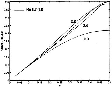
Figure 5: Lh(s) for methods using analytical derivatives instead of upwind differencing.
may be that certain additional error sources, related with the three-dimensionality or nonlinearity, destroy some of the advantages. Anyway, for usual panel densities the difference between finite differencing and analytical differentiation is only small.
Janson also considered the accuracy of a higher-order free-surface panelling. But as we already have seen, the discretisation of the raised source distribution only introduces negligible errors, and little can be gained. Correspondingly, the analysis yields hardly any effect on the accuracy for the raised-panel method. The increased computational effort therefore does not pay off. It is noted that the present linear analysis, for a linear FSBC imposed on the still water surface, does not permit to study the effect of the panel curvature, only that of the higher-order source distribution over the panels.
The foregoing analysis demonstrates that, why unusual, raised singularity methods can be very well analysed and the main properties are known for most of these. An exception may be formed by methods based on raised point sources, for which only a first and incomplete analysis has been published in [3]. One result obtained was that in that case the transverse distribution of the source points played a role, and a too large aspect ratio of the 2D source array could lead to important dispersion errors. This analysis deserves to be pursued.
3.5 A new low-damping difference scheme
The theoretical analysis has also been the key to the design of a novel difference scheme for the FSBC, which recently was introduced in RAPID. As noted above, for a conventional method the large first-order numerical dispersion inherent to the source discretisation is partly cancelled by a 3rd order dispersion due to the difference scheme. As a matter of fact, the Dawson scheme
has originally been selected for its favourable properties in the context of a conventional method [11]. Dawson simply selected the scheme based on inspection of 2D wave predictions, chose the 4-point scheme for its low damping, and took a 10% wavelength error for granted.
With the analysis available, it is possible to do better. The optimal scheme in a raised-panel context:
-
should introduce as little dispersion as possible (since there is no dispersion introduced by the source discretisation that needs to be cancelled);
-
should ideally cancel the slight numerical damping caused by the source discretisation for somewhat coarser panellings (s>0.08);
-
should retain the large damping at s>0.25 which is beneficial.
It is possible to design a 4-point upwind scheme that does exactly this. The ‘consistent’ 4-point backward scheme has a truncation error of ![]() and can be shown to introduce a negative numerical damping [17]. Dawson’s scheme, however, is a 4-point backward scheme with an error of
and can be shown to introduce a negative numerical damping [17]. Dawson’s scheme, however, is a 4-point backward scheme with an error of ![]() and gives a small positive damping. If third-order accuracy is sacrificed, a degree of freedom in the coefficients exists that permits optimisation of the scheme’s properties. The 4-point scheme can thus be tuned such as to produce near-zero numerical damping in combination with the raised-panel approach. Consequently, the optimal values of the coefficients are specific for the particular method used and the collocation point shift and panel elevation parameters. In practice, for panel elevations smaller than usual the coefficients should be adapted, but the form given below is near-optimal for all panel elevations exceeding α=0.8.
and gives a small positive damping. If third-order accuracy is sacrificed, a degree of freedom in the coefficients exists that permits optimisation of the scheme’s properties. The 4-point scheme can thus be tuned such as to produce near-zero numerical damping in combination with the raised-panel approach. Consequently, the optimal values of the coefficients are specific for the particular method used and the collocation point shift and panel elevation parameters. In practice, for panel elevations smaller than usual the coefficients should be adapted, but the form given below is near-optimal for all panel elevations exceeding α=0.8.
For reference, on a uniform grid the new scheme for the standard panel elevation is:
(20)
Fig. 6, which is a close-up of the low-s region of the graphs of ![]() compares various schemes, and shows that the new scheme has the desired property of yielding a near-zero total numerical damping over a range up to s≈0.125 (8 panels per wavelength). In addition, it leads to a 25% reduction of the numerical dispersion compared to Dawson’s difference scheme.
compares various schemes, and shows that the new scheme has the desired property of yielding a near-zero total numerical damping over a range up to s≈0.125 (8 panels per wavelength). In addition, it leads to a 25% reduction of the numerical dispersion compared to Dawson’s difference scheme.
Fig. 7 illustrates what happens if the special 3-point scheme we used up to now is replaced by the optimised scheme. Measured and computed longitudinal wave cuts, at 0.6L off the centreline, are compared for a slender vessel at Fn=0.33. The agreement with the data is already quite good for both calculations, but the small changes due to the new scheme almost all go in the direction of the data. Most notable is the improved representation of the short component at x/L=1.9. Further aft, the overestimation of the stern wave system,
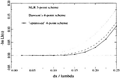
Figure 6: Numerical damping in raised-panel method with various difference schemes.
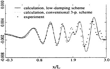
Figure 7: Longitudinal wave cut as measured and as calculated with conventional and new difference scheme. z/L=0.6, Fn=0.33.
which is due to the neglect of viscous effects, obviously becomes slightly larger.
Figs 8 and 9 shows a more critical case, for the same vessel at Fn=0.19. The vessel was sailing in a shallow channel with a sloping bank, and running out of the channel centre. The flow asymmetry, the panellings on the channel wall and bottom slope and the short, sharply diverging waves generated altogether made it hard to achieve full resolution even with the maximum number of panels (21000) possible on the CRAY. Nevertheless, a fair agreement is observed, except for the stern wave system that in this condition is quite strongly reduced by viscosity. There is a decisive improvement of the prediction of the maximum peak-to-trough wave height with the new difference scheme. At the tank wall it reduced the error by more than one half. More on these validations can be found in [18].
For the panel densities commonly used this elimination of numerical damping hardly gives any discernible effect close to the hull, but more at larger
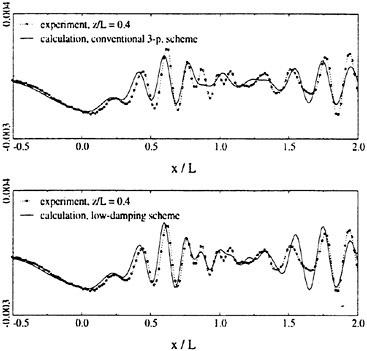
Figure 8: Longitudinal wave cut at z/L=0.4, Fn=0.19, for LIUTO vessel in shallow channel; with 3-point scheme (top) and with new low-damping difference scheme (bottom)
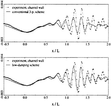
Figure 9: Wave cut at z/L=0.6 (channel wall) for LIUTO vessel in shallow channel; with 3-point (top) and low-damping difference schemes (bottom)
distances where a cumulative effect of the damping is found. The meaning of this development therefore is, either to permit a reduction of the panel density for equal accuracy, or to improve far-field predictions of wave amplitude; a topic of growing interest in view of fast ferry wash problems.
4 Resistance calculation
One of the practical aims of wave pattern calculations is obviously predicting the wave resistance. If not in an absolute sense, it may be quite useful in a comparative manner, answering the often posed question how much power is saved with a particular hull form modification.
First requirement here is a numerically accurate evaluation of the resistance from the calculated flow field, which is a known difficulty in wave pattern calculation methods. In the context of slow-ship linearised methods (Dawson’s method), attention has already been given to this, e.g. [19], partly inspired by the so-called ‘negative-resistance paradox’. This is a consequence of the fundamental disagreement between the wave resistance corresponding with the far-field wave pattern and that found from pressure integration over the hull [4].
Nonlinear methods remove this problem and in principle guarantee agreement of pressure integration over the hull, wave analysis and a control volume momentum balance. The problem of numerical accuracy, however, is slightly magnified in a nonlinear code. For consistency the hull pressure integration should extend over the actual wetted area under the wavy waterline. Consequently, the hydrostatic pressure contribution is non-zero over this area, and should be included in the integration. But at low Froude numbers, the hydrostatic pressure may be orders of magnitude larger than the hydrodynamic pressure, and any numerical integration errors or imperfections in the panelling may lead to drastic inaccuracies. Therefore, in RAPID and most likely in other codes, the integral of hydrostatic pressure under the still waterline (which should be zero) is subtracted again. Due to the wavy upper edge of the hull panelling, adapted to the free-surface panelling, this integration must separately treat partially wetted panels.
While an improvement in accuracy is thus obtained, the integrand of the pressure integration still may be relatively large, in particular for full hull forms. A second improvement is possible if the integral of the pressure in double-body flow is subtracted. Due to d’Alemberts Paradox, this again should be zero provided the hull is closed. Numerically it usually is not, due to numerical errors in the pressure calculation and integration. In view of the similarity of the double-body pressure distribution and that including the wave making, similar errors may be supposed to be present in the latter. Subtracting the double-body pressure integral obtained numerically thus eliminates part of the numerical errors in the wave resistance from pressure integration. As a matter of fact, this double-body flow correction was found to reduce the dependence of the pressure integration resistance on the hull panel distribution for critical cases.
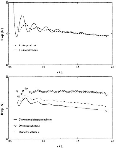
Figure 10: Wave resistance found from transverse cut analysis of predicted wave pattern. Dyne tanker at Fn=0.165. Top: Wavy dependence on x-position of cuts, removed by spreading the wave cuts. Bottom: Effect of low-damping difference scheme on slope of Rwp(x)-line.
There are two complications here. One is again the waviness of the hull panelling, which therefore does not permit a simple mirroring in the still waterplane. This difficulty has been overcome by writing a special double-body flow postprocessor, which simply cuts off the hull panelling along the still waterline, and uses the resulting (partly irregular) hull panelling to compute the double-body flow. The second complication is that d’Alemberts Paradox only applies to closed bodies, and therefore this procedure cannot be applied to cases with a transom stern that (including dynamic trim and sinkage) extends below the still water level.
Altogether, with these corrections it usually appears possible to determine the wave resistance by hull pressure integration well enough to compare design variations, except for blunt hull forms. For an average containership or ferry there should be no problem.
An alternative to the hull pressure integration is wave pattern analysis. This technique has been developed in the framework of the EC-funded CALYPSO project, and is now being used as a postprocessor for RAPID. It is based on analysis of a number of transverse cuts through the calculated wave pattern aft of the vessel. The position of these cuts should have no effect on the result, as long as they are outside the near-field disturbance. However, as discussed in [20], a pronounced wavy dependence of the wave pattern resistance on the longitudinal position was found (Fig. 10). We could show that this waviness is due to the application of an essentially linear analysis to a wave pattern including all nonlinearities. It can and may be removed by spreading the cuts over a transverse wavelength, as is motivated in [20].
However, doing so we obtain a wave pattern resistance that decreased monotonously with distance aft of the hull. The slope of the line appeared to be closely correlated with the numerical damping as found from the accuracy analysis in Section 3. Fig. 10 shows the dramatic improvement obtained if the new low-damping difference scheme is applied. The wave pattern resistance so evaluated is almost independent of x as it should, is in much closer agreement with the result of pressure integration over the hull, and is stable enough to serve for comparing design variations.
As an alternative to wave pattern analysis, integrating the momentum flux over a control volume might be a better option, being unaffected by nonlinearities and having an integration accuracy that is better controllable than integration over the hull. This will be tested in a near future.
5 Stern flow prediction
In Section 2 we have paid some attention to the modelling of the flow off a transom stern. Evidently, without ad-hoc modifications all potential flow methods can only represent a smooth inviscid flow off the transom, not a ‘dead-water’ area aft of the transom. While different implementations are being used by different nonlinear methods, there is agreement that the smooth transom flow is governed by the tangential flow off the hull and the dynamic condition at the transom edge.
In the past, mainly in the context of linearised methods, some quite different flow models have been proposed. Some have argued that vortex shedding is a dominant mechanism in transom flows, and have denoted the transom conditions a ‘Kutta condition’. In [4, 13] it has been argued that this is an erroneous notion of what happens; and that the conditions to be imposed in a nonlinear method are basically straightforward. Anyway, there is sufficient reason to validate the transom flow predictions.
However, such validations have only rarely
Figure 11: Typical calculated transom flow pattern
been carried out, presumably because of the difficulty to measure wave elevations in the path of the model. A few years ago, MARIN has done tests for a frigate, in a project commissioned by the Royal Netherlands Navy, in which a centreline wave cut aft of the transom has been measured. A special wave height pickup was used, attached to a subcarriage running along a longitudinal rail fitted to the towing carriage. Measurements have been done at different trim conditions, such that the whole range of smooth flows off the transom was covered. The validations, published in [14], indicated that the modelling used in RAPID correctly indicated the variation of the stern wave height and shape with transom edge height, and reasonably well indicated the dependence of wave resistance on trim as far as could be judged from the data. But for the steeper stern waves (larger transom immersion/lower speed) the program predicts a too rounded wave with a crest slightly too far aft. This makes the agreement qualitative rather than quantitative. This deviation has been found to be quite systematic, and is attributed to the neglect of viscous effects. Support of this supposition is found in [21].
Many new experimental data are now being collected, mainly in the framework of the EC-funded CALYPSO project. For various merchant vessels, normal longitudinal cuts and centreline stern wave cuts at varying trim or draft are being measured and will be compared with the predictions of both SHIPFLOW and RAPID. Main objective here is to determine limits of validity of the inviscid flow model; or more specifically: to what extent an inviscid transom flow model gives the right design indications, while in reality a viscous boundary layer leaves the stern at the transom, or even some wave breaking and a thin layer of dead water is present aft of the transom. These obviously are extremely important questions from the practical point of view: Such flow types are quite common in practice, and a proper transom stern design often has been found to yield appreciable power savings.
We shall now show some relevant validations
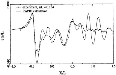
Figure 12: Measured and calculated longitudinal cuts for a dredger, Cb=0.80, Fn=0.22.
carried out for RAPID during the last few years. Fig. 12 is for a full hull form at relatively high Froude number. Extensive wave breaking was observed at the deep wave trough at the forebody, which explains the much shallower trough in the experiment. Also the deviations directly aft of this may be connected with the breaking. But there is a large overestimation of the stern wave system. In the calculation the flow is supposed to clear the transom, but in reality obviously the viscous, perhaps separated flow has lost much of its momentum and is unable to reduce the pressure at the transom edge to atmospheric level. A dead water region aft of the transom results, and there is a drastic disagreement of the stern wave height.
In other situations, the free surface detaches from a smooth part of the hull. This happens for a cruiser stern, or for a transom too high above the wave surface. Experience so far suggests that also this type of flow is strongly influenced by viscous effects, in particular if the boundary layer thickens due to a wetted section girth decreasing aft. A potential flow model invariably overestimates the stern wave system in such cases. An example is Fig. 8.
Fig. 13 compares measured and longitudinal wave cuts for a fast ferry with a wide flat transom, a project carried out for Kvaerner Masa Yards. The cuts are taken just outside the hull. The agreement is quite good along most of the hull, including the first part of the stern wave. However, the prediction underestimates the second peak that occurs at x/L=0.7, and overestimates the wave amplitude further aft. Observation of the tests revealed that the second peak was due to a diverging, slightly breaking wave originating at the centre of the transom. While wave breaking is not included in the mathematical model anyway, the direct cause of this local phenomenon may here have been the viscous wake
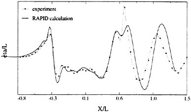
Figure 13: Measured and calculated wave cuts for a fast ferry at Fn=0.30.
of a skeg just forward of the transom edge. The reduced flow velocity in the wake leads to a flow emerging more steeply aft of the transom edge, in this case leading to slight breaking. The overestimation of the stern wave amplitude further aft probably is a more general result of the viscous losses along the hull.
The same vessel has been tested with a short and long ducktail (i.e. a small extension of the bottom of the hull, protruding aft of the transom). Fig. 14 shows the measured and the predicted effect of these local stern modifications on the wave cuts. It appears that the trend of the stern wave is well captured qualitatively. However, the effect on the wave amplitude further aft is overestimated. It may be that dissipation by the wave breaking here plays a role. Nevertheless, the relative reductions of the residual resistance achieved with the two ducktails were almost exactly predicted: 21% and 35% according to RAPID; 24% and 33% measured.
Finally, Fig. 15 shows the experimental and computational comparison of two design variations of the LIUTO vessel [18], differing primarily in the shape of the stern. The effect of the hull form changes on the wavemaking is very well captured by the code, including the detailed differences in the trailing stern wave system.
These examples illustrate our experience that a proper inviscid model for the flow past the afterbody and off the transom can give very useful results and good design indications in a range of flows; in particular for fairly slender vessels with smooth stern lines and a relatively flat transom, designed such that a reasonably smooth flow off the stern takes place. However, with experience even the less valid predictions can be used effectively to design a better stern shape. E.g. a steeply rising ‘rooster tail’ aft of the transom in a calculation often will mean substantial dead water in reality; a calculated stern wave curving downward soon after leaving the transom edge suggests that the transom is too high

Figure 14: Measured (top) and calculated (bottom) effect of ducktails on wave cut. Fast ferry, Fn=0.30.
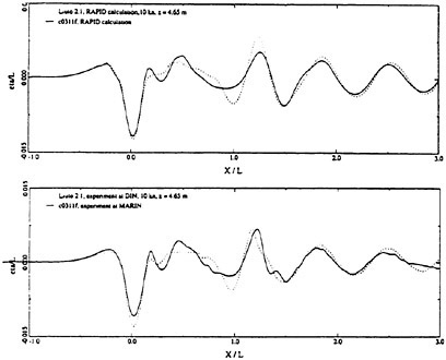
Figure 15: Accuracy of predicted differences between two variations of the LIUTO design at Fn=0.33. Predicted (top) and measured (bottom) longitudinal cuts.
and draws the wave surface upward. The behaviour in such cases would be quite hard to predict or anticipate by other means.
The statement is sometimes made that potential flow calculations are of use only for forebody optimisation. While this was largely correct for linearised methods, it is far too pessimistic for nonlinear methods. All the same there are some classes of flows for which a due account of viscous effects on the wavemaking, or even a coupled RANS/FS solver, is necessary to produce useful predictions.
The same goes for resistance predictions. While a numerically accurate prediction of the inviscid wave resistance is feasible at least for not too full hull forms (see the previous section), the overestimation of the stern wave system inherent to the neglect of viscosity will always cause an overestimation of the wave resistance. According to current experience, the error varies from zero for slender vessels at higher speed, to perhaps 100% for full-shaped vessels with separation or a thick boundary layer at the stern. Without any correction for these effects, a performance prediction based on a wave pattern calculation will remain a risky affair. Except for quite slender vessels, the use of the predicted wave resistance will thus be limited to comparisons of hull form variations, provided these do not significantly affect the viscous/inviscid interaction at the stern. The optimisation study in [22] illustrates what may happen if the latter condition is violated.
6 Capabilities and limitations
Section 2 has compared the technical content of the leading nonlinear ship wave pattern calculation methods and has indicated that these are based on fairly similar approaches. Differences are mainly in implementation details, which, however, can have a substantial effect on convergence and accuracy.
Section 3 discussed a theoretical analysis of the effect of the discretisation, difference scheme and some of the parameters involved, and demonstrated that all these can be well controlled and optimised. The new difference scheme designed for RAPID was just one demonstration of the benefits of the analysis.
Sections 4 and 5 addressed two other critical points of this class of methods, and has indicated that improvements are being made but that some problems are fundamental to the inviscid flow model and will not be removed.
We shall now concisely sum up the main capabilities and limitations of the nonlinear free surface potential flow model, based on available experience and validations.
6.1 Capabilities
Nonlinear free surface potential flow methods like those discussed in this paper are able
-
To accurately predict the near field of the wave pattern and flow around almost the entire hull, for all usual ships at speeds more or less in agreement with normal shipping practice. Contrary to linearised methods, with sufficient resolution nonlinear methods can accurately predict the bow wave height and the amplitude of the diverging bow waves.
-
To provide much other information useful for design, such as streamlines, pressure distributions, dynamic trim and sinkage.
-
To incorporate the effect of hull form features above the still water line, such as bow flare, bulbous bows piercing the water surface at rest and stern overhangs.
-
To predict trends of the wave making with variation of the afterbody and transom design, for more or less slender vessels and subject to some restrictions (see below); thus permitting large power savings. To provide useful information on the quality of the afterbody design even for fuller vessels.
-
To accurately indicate the effect of most other hull form changes on the wave making and, with restrictions, on the wave resistance.
-
To predict the wave pattern in shallow water at sub- or supercritical speeds; although only the former have been validated so far. Also the shallow water effect on the flow around the hull is obtained.
-
To predict the effect of channel walls, and wave amplification due to wave propagation into shallow water, although limited by unsteadiness [18].
-
To give accurate predictions of catamaran wave patterns and resistance, trim and sinkage; including quite good predictions of the wave interference effect on these quantities.
-
To predict the flow around hydrofoils near the free surface, thereby eliminating any doubts on the validity of linearised FSBC’s.
6.2 Limitations
It (currently) appears to be impossible:
-
To make a quantitatively accurate prediction of the trailing stern wave system for all but the most slender vessels, as a result of the neglect of viscous effects. The largest deviations are found for dead water flow aft of the transom, detachment from smooth parts of the hull surface, converging stern shapes (leading to accumulation of the boundary layer) and more generally for full stern shapes.
-
To make a quantitatively accurate prediction of the wave resistance in all cases in which the stern wave amplitude is overestimated due to viscous effects.
-
To predict whether the flow off the transom stern will be smooth, will have a spilling breaker or will have a region of dead water. This is a most unstable process dependent on factors not included in the potential flow model used.
-
To predict differences in resistance between design variations if these variations lead to a significantly different viscous/inviscid interaction at the stern [22].
-
To predict the effect of wave breaking on the wave pattern; and even to produce a converged inviscid solution for cases displaying heavy wave breaking in reality, possibly because of the nonexistence of a steady potential flow solution without additional dissipation. Some research on artificially removing this difficulty is being done [23].
-
To predict wave wash at large distances from the hull, due to the memory requirements of the code and the accumulation of damping and dispersion effects. This difficulty in principle can be removed by a composite approach with an analytical representation of the outer field; the memory restriction can be relieved by the use of domain decomposition or multipole methods.
7 Status and prospects
A decade of development and use of the main nonlinear free surface potential flow methods has produced codes that provide outstanding services as a design tool. Predicting the inviscid flow past the hull nowadays is a quick and efficient procedure and provides a comprehensive view of the flow properties. This paper contains several indications of which part of these predictions is reliable and which is not. Provided the results are sensibly considered, analysed and interpreted, much more can be done than is commonly thought. We definitely do not share the opinion that inviscid flow methods are useful for forebody design only.
Compared to linearised (Dawson-type) methods, a large step forward has been made in the quantitative accuracy of the predictions (including the wave resistance). Still several aspects are just useful in a comparative sense rather than for e.g. performance prediction. As indicated above, this is largely fundamental to the basic flow model.
Expected further development of this class of codes may provide an even larger computational efficiency, due to introduction of improved numerical algorithms; will lead to a further introduction of the codes at consultants and shipyards; and will make the codes even more generally applicable by basically straightforward extensions (multihulls, lifting surfaces, ships in channels, etc.). Little further development on the basics is expected.
Progress regarding the issues listed as ‘limitations’ in the last section largely relies on modelling the viscous effects on the flow and wavemaking. Simple corrections for these might lead to a better agreement with experiments but generally will be too crude to distinguish between similar designs having different viscous flow behaviour. Improvement will perhaps only be obtained by RANS solvers with free surface boundary conditions. The present intensive research in this area may thus remove some of the principal shortcomings of the methods discussed here. However, this will require a substantial improvement of the resolution in the first place, to remove the present inability to predict all but the larger-scale waves. Moreover, the RANS/FS methods ideally should include a proper model for the detachment of the free surface from a smooth part of the hull surface; and of the generation of a dead-water flow aft of a transom. In view of the physical sensitivity (near instability) of the latter this will be a major challenge.
Consequently, for some time to come inviscid flow models may remain the leading tool in hull form design for low wave making. There is still a key role for the naval architect having extensive experience with the code, having insight in the physics, and frequently observing model tests. “The purpose of computation is insight, not numbers”. For providing such insight, nonlinear free surface potential flow codes are still hard to beat.
Acknowledgment
Kvaerner Masa Yards are thanked for their permission to publish Figs 13 and 14; Carl-Erik Janson of Flowtech for his permission to copy Figs 1 and 5.
References
[1] Jensen, G., Mi, Z.-X., and Söding, H., “Rankine source methods for numerical solutions of the steady wave resistance problem”, Proc. 16th Symp. Naval Hydrodynamics, Berkeley, 1986.
[2] Jensen, G., “Berechnung der Stationären Potential-strömung um ein Schiff unter Berücksichtigung der nichtlinearen Randbedingung an der Wasseroberfläche”, Thesis, IfS Bericht 484, 1988.
[3] Raven, H.C., “A Practical Nonlinear Method for Calculating Ship Wavemaking and Wave Resistance”, 19th Symp. Naval Hydrodynamics, Seoul, South-Korea, 1992.
[4] Raven, H.C., “A solution method for the nonlinear ship wave resistance problem”, Doctor’s Thesis, Delft Univ. Techn., Delft, Netherlands, 1996.
[5] Ni, S.-Y., “Higher-order panel methods for potential flows with linear or nonlinear free-surface boundary conditions”, Ph.D. Thesis Chalmers University, Göteborg, Sweden, 1987.
[6] Kim, K.J., “Ship flow calculations and resistance minimization”, Ph.D. Thesis Chalmers University, Göteborg, Sweden, 1989.
[7] Janson, C.-E., “Potential flow panel methods for the calculation of free-surface flows with lift,” Doctor’s Thesis Chalmers University, Göteborg, Sweden, 1997.
[8] Hughes, M.J., “Application of CFD to the prediction of wave height and energy from high-speed ferries”, Int. CFD Conference, Ulsteinvik, Norway, 1997.
[9] Rosen, B.S., and Laiosa, J.P., “SPLASH nonlinear and unsteady free surface analysis code for Grand Prix yacht design’, 13th Chesapeake Sailing Yacht Symposium, 1997.
[10] Daube, O., and Dulieu, A., “A numerical approach of the nonlinear wave resistance problem”, 3rd Int. Conf. Numerical Ship Hydrodyn., Paris, 1981.
[11] Dawson,C.W., “A Practical Computer Method for Solving Ship-Wave Problems”, 2nd Int. Conf. Numerical Ship Hydrodyn., Berkeley, 1977
[12] Jensen, P.S., “On the numerical radiation condition in the steady-state ship wave problem”, Journal of Ship Research, Vol. 31–1, 1987.
[13] Raven, H.C., “Nonlinear Ship Wave Calculations using the RAPID Method”, 6th Int. Conf. on Numerical Ship Hydrodyn., Iowa City, USA, 1993.
[14] Raven, H.C., and Valkhof, H.H., “Application of nonlinear ship wave calculations in design”, Symp. Practical Design of Ships and Floating Structures, Seoul, Korea, 1995.
[15] Sclavounos, P.D., and Nakos, D.E., “Stability analysis of panel methods for free-surface flows with forward speed”, Proc. 17th Symp. Naval Hydrod., Den Haag, Netherlands, 1988.
[16] Bunnik, T.H.J., and Hermans, A.J., “Stability analysis for solving the 3D unsteady free-surface condition with raised panels”, 13th Int. Workshop on Water Waves and Floating Bodies,, Alphen a/d Rijn, Netherlands, March 1998.
[17] Strobel, K.H., and Cheng, B.H., “Finite difference operators for the Rankine source method”, OMAE Conference Vol. I-A, Offshore Techn., 1992.
[18] Raven, H.C., Van Hees, M., Miranda, S., and Pensa, C., “A new hull form for a Venice urban transport waterbus—design, experimental and computational optimisation”, 7th Symp. Practical Design of Ships, The Hague, Netherlands, 1998.
[19] Raven, H.C., “Adequacy of Free-Surface Conditions for the Wave-Resistance Problem”, 18th Symp. Naval Hydrod., Ann Arbor, 1990.
[20] Raven, H.C., and Prins, H.J., “Wave pattern analysis applied to nonlinear ship wave calculations”, 13th Int. Workshop on Water Waves and Floating Bodies,, Alphen a/d Rijn, Netherlands, 1998.
[21] Haussling, H.J., Miller, R.W., and Coleman, R.M., “Computation of high-speed turbulent flow about a ship model with a transom stern”, Report CRDKNSWC/HD-0200–51, Naval Surface Warfare Center, Sept. 1997.
[22] Janson, C.-E., and Larsson, L., “A method for the optimization of ship hull forms from a resistance point of view”, 21st Symp. Naval Hydrodynamics, Trondheim, Norway, 1996.
[23] Subramani, A.K., Beck, R.F., and Schultz, W.W., “Suppression of wave-breaking in nonlinear water wave computations”, 13th Int. Workshop on Water Waves and Floating Bodies,, Alphen a/d Rijn, Netherlands, March 1998.
DISCUSSION
H.Chun
Pusan National University, Korea
1. In your earlier published papers, you mentioned that a relaxation factor is necessary to get the converged solution. Is it necessary still? If yes, how is the dependency of the solution?
2. It has been known that the collocation point shift method can improve the errors in the dispersion and damping compared to the FDM. In your RAPID method or your study, have you tried to use the collocation point shift method instead of using the 4-point finite-difference scheme?
3. The double-body approximation, called the Dawson method, is based on the very slow speed assumption and so the method is made applicable, in principle, to the slow speed problem. For the high-speed ships such as a ship with transom stern, the Kelvin type free-surface boundary condition is more likely in physics. What do you think on that?
AUTHOR’S REPLY
1. Underrelaxation is useful in the iteration for the nonlinear solution for harder cases. The change from one iteration to another is multiplied with that factor. The final solution does not depend on it at all.
2. I have not tried the collocation point shift method in RAPID. It means a rather comprehensive change of the code, requiring the calculation and storage of induced second derivatives of the potential as well, and other changes. As mentioned in my paper, a comparison has been made by Janson, who found no appreciable improvement in test calculations using collocation point shift.
3. Slow-ship linearization is not strictly limited to slow ships, as has been found in practice. Fast ships are usually slender, so the double-body flow does not differ much from a uniform flow, and the slow-ship linearized condition is close to the Kelvin condition. Thus Dawson’s method still may work fairly well. There are, however, exceptions, such as hydrofoils near the free surface. For transom flows (evidently not limited to high-speed ships), any standard linearization is inadequate. Of course, any doubts on the validity of linearizations are irrelevant for the nonlinear methods that are the subject of my paper.
Free Surface Flow Analysis of Fins Attached to a Strut and Foils by a Higher Order Boundary Element Method
C.Lee,1 I.-R.Park,2 H.-H.Chun,2 S.-J.Lee1 (1Pohang University of Science and Technology,2 Pusan National University, Korea)
ABSTRACT
An experimental and numerical investigation of the lift and flow characteristics of a submerged pair of fins attached to a strut and also fin alone is carried out. The objective of the investigation is to validate a numerical method which can predict the effect of the free surface and struts on the lift characteristics of fins. The experimental and numerical results are compared and pertinent discussions are made. The results reveal that the free surface effect becomes significant when the depth of submergence to chord ratio (H/c) is less than three. The effect of the strut is also realized for shallower depth of submergence of the fins through free-surface deformation leading to a significant change in the incidence angle of the flow to the fins. The numerical results based on the High Order Boundary Element Method with linearized free surface condition show good agreement with the experimental results for fin (foil) alone even at shallow submergence but some discrepancies exist between the computed and experimental resutls for the fin attached to the strut at higher speeds, which appears to be mostly due to the neglect of the non-linear free surface effect.
1. INTRODUCTION
For high-speed ships to maintain the stability and speed in rough ocean environments, some means of controlling the wave-excitation motion are necessary.
Among various device for the motion control, fins have been recognized as a very effective one such as in maintaining stability of submerged vehicles and air-flight projectiles. To a certain degree, the lifting characteristics of fins have been reasonably well predicted by some semi-empirical formulae shown, for instance, by Whicker et al. (1) and Pitt et al. (2). For the fins attached to surface ships, the lifting characteristics can be significantly altered due to the effect of the free surface.
There have been numerous investigations on the effect of free surface on submerged foils of large aspect ratio (Wu (3), Breslin (4), Nishiyama (5), Nakatake (6), Bai & Lee (7)); however, similar investigations on fins attached to a body are scarce. Ohmatsu et al. (8) investigated the lift characteristics of the fins attached to a semi-submerged ship in calm water and wave conditions. Mori et al. (9) and Qi & Mori (10) carried out numerical and experimental investigation on the resistance and flow characteristics of semi-submerged ships with wings.
The aim of the present investigation is to validate the numerical method based on a Higher Order Boundary Element Method (HOBEM) to predict the combined and separate effects of free surface and body on the lift characteristics on a pair of fins attached to a strut. The choice of a strut is for the geometric simplicity for investigating the effect of body on the fins. The variables involved in the investigation are the ratio of depth of submergence to chord length of the fin, the angle of attack of the fins, and the free-stream velocity. The Kelvin linearized free-surface condition is used. The effect of viscosity and cavitation is not taken into account. A simple Rankine Source is employed and, to improve the accuracy of the solution and convergence state, the bi-quadratic scheme of Sclavounos and Nakos (11) which is extended to 9-node Lagrangian curved elements on the free surface is used.
Experimental investigation is carried out using a circulating water channel with a pair of fins of rectangular plane of aspect ratio of 1.2 with the NACA-0015 foil shape attached to a vertical strut of rectangular cross section faired with elliptic ends. The validation of the numerical method is checked by comparing the numerical and experimental results.
2. MATHEMATICAL FORMULATION
A right-handed Cartesian coordinate system is used with the origin located on the free surface
z=0, the positive x-axis in the direction of the free stream, and the z-axis directed upward. The fluid is assumed to be inviscid, incompressible, its motion irrotational, and free of surface tension. With this assumption, the velocity potentail Φ(x, y, z) is introduced and the governing equation in the fluid domain becomes Laplace equation,
(1)
The velocity potential Φ(x, y, z) may be decomposed into the uniform stream part and the velocity potential ![]() representing the disturbance by the body, strut, and free surface as follows:
representing the disturbance by the body, strut, and free surface as follows:
(2)
Boundary conditions to be satisfied on each boundary surface are as follows:
Linearized free surface condition on the free surface;
(3)
where g is the gravitational acceleration and U∞ the free-stream velocity.
Body boundary condition;
(4)
where nx is the x-component of the unit normal vector pointing out of the fluid domain, on the body surface SB.
Far-field condition;
(5)
Kutta condition at the trailing edge of a hydrofoil;
(6)
It is assumed that the trailing wake surface SW generated by the fins is flat and on SW,
(7)
where subscripts U and L are the upper and lower surfaces of the wake and V and p are velocity and pressure, respectively.
Integral equation
The velocity potential ![]() which is the solution of the Neumann-Kelvin problem can be written as an integral equation by the Green’s Theorem,
which is the solution of the Neumann-Kelvin problem can be written as an integral equation by the Green’s Theorem,
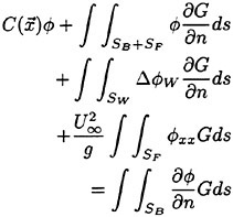
(8)
where ![]() collocation point,
collocation point, ![]() potential jump on the wake,
potential jump on the wake,
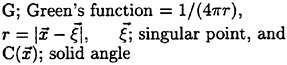
3. NUMERICAL METHOD
In general, panel methods have been widely used to calculate flows around an arbitrary body with singularity distribution on the boundary surfaces. By comparison with the conventional panel methods, the boundary surfaces and physical quantities in HOBEM are represented by curved elements of the second order (or even higher) and a shape function of the same order, respectively.
The accuracy and numerical convergence of the computational results by HOBEM are thus expected to be improved. In the present paper, the body boundary surfaces and physical quantities are represented by a 9-node Lagrangian shape function and on the free surface, the geometry is represented by a 9-node Lagrangian element and the physical quantities by a bi-quadratic spline function which has an advantage of the continuity in physical quantities across the neighboring elements. The purpose of introducing the spline function into the calculation of the velocity potentials on the free surface is to remove a numerical wave damping and to improve the wave dispersion property, which would lead to a better solution. Sclavounos & Nakos (11) showed the advantage of this approach by comparing with other schemes. They used their own radiation condition which will be mentioned later.
Boo (12) used a 16-node cubic order Lagrangian shape function on the free surface. The order is higher than the bi-quadratic spline function, but it appears that a discontinuity in the physical quantities across the neighboring element could cause a divergent solution. It was observed from the results
in the paper that it would be difficult to get a converged solution, especially, for a shallowly submerged body and a surface piercing body.
9-node Lagrangian element method; Fig. 1a shows local coordinates system for a boundary element and Fig. 1b shows a general 9-node element and a discontinuous element for an edge problem or singular point which has different boundaries. Boundary surfaces and physical quantities are represented by a 9-node Lagrangian shape function as follows:
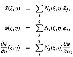
(9)
where Nj(ξ, η) is the shape function.
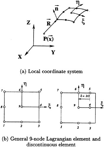
Fig. 1 Description of numerical grids
Bi-quadratic spline method: The physical quantities on the free surface are represented by bi-quadratic spline function as follows:
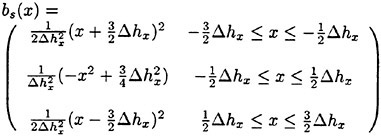
(10)
where Δhx is the length between neighboring elements.
The bi-quadratic spline function normalized on a mapped plane, −1≤ξ≤1, is as follows:
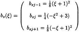
(11)
The velocity potential on the free surface is represented by the normalized bi-quadratic spline function as

(12)
where ![]()
![]() and φk is a weighting coefficient at the centroid of the k-th element. NF is the number of total elements and NFY is the number of elements in y-direction on the free surface.
and φk is a weighting coefficient at the centroid of the k-th element. NF is the number of total elements and NFY is the number of elements in y-direction on the free surface.
Then, the following equation can be obtained from Equation (8):

(13)
where J is the Jacobian of the coordinate transformation. NB and NW are the number of elements of the body and wake surface, respectively. The superscript e denotes an element of the surface.
A standard Gauss-Legendre quadrature is used for the evaluations of the integral equations and the singular integrals are regularized by introducing nonlinear coordinates transformation technique by Telles (13).
Radiation Condtion
Sclavounos and Nakos (11) used the following equations at the upstream truncation boundary for a radiation condition.
(14)
The above equation can be transformed into φi−1=φi=φi+1 at the upstream truncation boundary for the bi-quadratic spline function method where subscript is the position of neighboring three elements in the down-stream direction and at the lateral boundary it can be imposed that the second derivative in y-direction of the velocity potential may be zero.
The Kutta Condition
Discontinuous elements are used to avoid the evaluation of integrals in the plane where three planes with different physical values are meet. Then, the Kutta condition is imposed at some points on the surface of a fin away from the trailing edge. A pressure Kutta condition by Lee (14) was employed in the present study and this has been used efficiently for the three dimensional problems such as foil and propeller for the uniqueness and convergence of the solution.
4. EXPERIMENTAL METHOD
The strut and the fin used in the present investigation are shown in Fig. 2. The basic cross section of the strut is rectangle of 500 mm in width, 50 mm in thickness and 1300 mm in length. The fore and aft ends of the horizontal cross section is faired by an ellipse of 2 to 1 ratio between the major and minor axes. The fin is of NACA-0015 foil shape with a rectangular plane form of 100 mm in chord (c) and 120 mm in span. The material of the strut and fin is aluminum.
The fins can slide vertically along the groove of 20 mm in width which is made in the mid-width of the strut. Once the fins are positioned at the desired vertical position, the groove is filled flush with the strut surface with stylofoam and acrylic materials. The angle of attack of the fins can be adjusted between ±20 degrees. A load cell is attached on top of the vertical axis at which the fins are attached with a horizontal rod. The load cell is designed to measure the vertical force acting on the fins only.
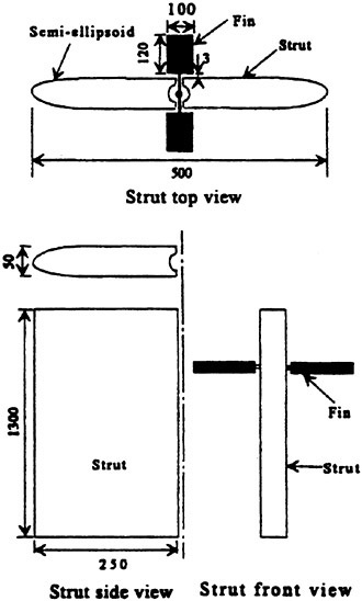
Fig. 2 Fin and strut configuration: unit in mm
The experiment was carried out in a circulating water channel of test section of 1 m in depth, 1 m in width and 4.53 m in length. The maximum flow velocity the channel can generate is 2.2 m/s. The blockage ratio of the strut-fin structure was about 5% such that no correction was necessary for the blockage effect on the measurements according to Goldstein (15).
The experimental parameters in the present investigation are the depth of submergence of the fins i.e. the vertical distance from the calm-water surface to the center of the mean chordline, H, the angle of attack of the fins, α, and the free stream velocity, U∞. The definition of these variables is given in sketch in Fig. 3, and the values of the parameters chosen in
the experiment are as follows:
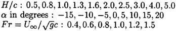
where c is the chord length of the fins. In the present case ![]() and hence the Froude number is identical with U∞ in m/s. For c=2 m Fr=1.5 corresponds to about 19 knots. Thus, the Froude numbers considered in the present experiment are in low-speed range for high-speed ships of 25 to 35 knots cruising speed. Such a choice is forced by the limitation of the test facility.
and hence the Froude number is identical with U∞ in m/s. For c=2 m Fr=1.5 corresponds to about 19 knots. Thus, the Froude numbers considered in the present experiment are in low-speed range for high-speed ships of 25 to 35 knots cruising speed. Such a choice is forced by the limitation of the test facility.
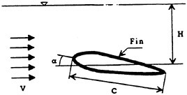
Fig. 3 Definition of variables
To investigate the lift characteristics of fins alone, the pair of fins were joined together and supported by a right-angled streamlined strut which is attached to the mid-span of the trailing edge. Thus, the disturbance of the flow by the strut was minimized.
The measured quantities are the lift force, L, which is represented in terms of the lift coefficient, ![]() where ρ is the density of the water and A the plane area of the two fins, and the wave profiles along the side of the strut and on the extended centerline aft of the strut.
where ρ is the density of the water and A the plane area of the two fins, and the wave profiles along the side of the strut and on the extended centerline aft of the strut.
The longitudinal-plane section of the flow at the mid-span of the fin and the extended centerline of the strut aft of its trailing edge as shown in Fig. 4a, was visualized using the laser light sheet technique to investigate the variation of the free surface elevation. Fig. 4b shows the schematic diagram of experimental set-up for the flow visualization experiment. In this experiment, a beam of 4W Argon-ion laser was irradiated on the cylindrical lens immersed behind the fin, by which it was spread into a two-dimensional laser light sheet. The wave patterns in the plane of the light sheet were recorded using a Nikon F5 camera installed on an optical rail located outside the water channel. The visualized photos were digitized with a scanner and the free surface wave profiles were extracted from the photographic images with the help of digital processing technique using a Photoshop software.
In order to check the reliability and usefulness of the photo-image technique, the wave heights at several locations in the extended centerline aft of the strut were measured by a capacitance type waveheight gauge and compared with those measured using present image processing technique. The comparison results shown in Fig. 5 are in good agreement with each other. The wave height measured with present technique near the wave crest appeared larger than that from the wave height gauge. This may have resulted from the deflection of laser light due to high curvature of the free surface at the crest at x/L=1.0, where L is the strut length.
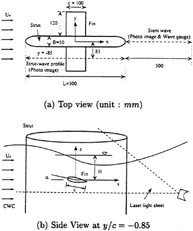
Fig. 4 Schematic diagram of experimental set-up
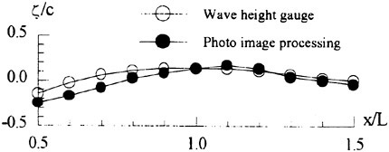
Fig. 5 Comparison of free surface configuration without fin at strut middle section (Fr=1.2)
From the experiments, the digital imaging prcessing technique was proven to be a useful and
powerful tool for capturing the instantaneous wave profile in the plane of light sheet.
5. RESULTS AND DISCUSSIONS
The measured values of lift coefficient CL of the fins attached to the strut versus the submergence ratio, H/c, for the angle of attack (α=0°, 10°) for the Froude numbers ranging from 0.4 to 1.5 are shown in Fig. 6. The lift force of a symmetric foil in unbounded flow would be zero at α=0°. However, the lift coefficient of a foil attached to a strut at α=0° in the presence of the free surface is considerably varying with the free stream velocity and the fin submergence depth due to the effects of the free surface and the strut.
The results show that the free-surface effect on CL is greater for smaller depth of submergence and for greater free-stream velocity, as anticipated. The free surface effect seems to increase significantly in the Froude number range between 0.8 and 1.2 for H/c≤3.0. The negative CL is due to the fact that the strut-induced incidence angle of the flow to the fin happens to be negative. However, the apparent reverse trend of CL versus H/c at Fr=0.8 is interesting due to the reversed incidence angle of the flow and these are discussed later in detail together with the wave profile comparisons.
As the submergence depth increases for the α=0° case, the lift coefficient also increases and tends to converge to the value of the unbounded case. Such a trend changes depending on free stream velocity and fin angle of attack. As shown in Fig. 7 which shows the CL variation versus H/c at various angles of attack at two speeds, Fr=0.6 and 1.5, CL converges to a constant value at around H/c=2.0 for a relatively slower speed of Fr=0.6, but it increases as H/c increases at a higher speed of Fr=1.5 although the gradient seems to be small for H/c>3.0.
The comparison of the experimental results with the computed results for CL versus H/c for the fins attached to the strut for α=0° and 5° is shown in Fig. 8. The results of the four representative Froude numbers i.e. Fr=0.4, 0.8, 1.2 and 1.5 are chosen for comparison. Sufficient numbers of convergence tests on the numerical results with respect to the computational domain and also element numbers are performed. It is found that 286 elements for the half of the strut attached with the fins and 840 elements for the free surface of −1≤ x/L≤2 and 0≤y/L≤1 are sufficient to obtain a converged solution. For the case of α=0°, the agreement betweent the two resutls at Fr=0.4 and 0.8 is fairly good while some discrepancy can be seen for the higher speeds. It is worthwhile noting that the numerical result predicts well the trend of the positive increase in CL with the decrease of H/c at Fr=0.8. For the case of α=5°, the numerical results are lower than those of the measurements for all speeds, whereas the similar discrepancy can be seen only for Fr>0.8 for the case of α=0°. The fluctuation in the measured CL values at the slower speeds indicate some difficulty in the measurement in the circulating water channel partly due to the inherent flow non-uniformness and also partly due to the small magnitude of the lift forces.
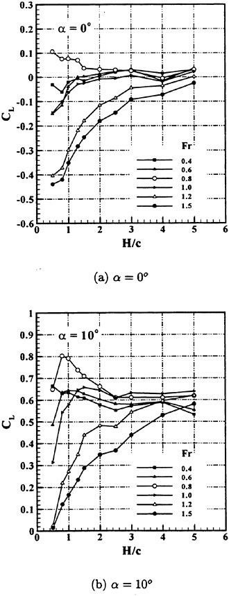
Fig. 6 Experimental results of lift coefficients versus submergence ratio for fins attached to strut
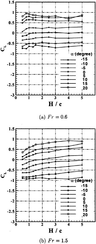
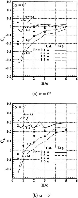
Fig. 9 shows the computed and measured CL versus angle of attack for the fins attached to the strut at H/c=1.0, 2.0, and 5.0. The computed and measured CL for the fins alone at H/c=1.0 and 3.0 is shown in Fig. 10. It can be seen in Fig. 9 that shallower the depth of submergence and greater the speed, the discrepancy between the computed and measured results increases. The lift curve slope for the fins-alone case computed by the formula of Whicker and Fehlner (1) is 2.76 while the corresponding measured results shown in Fig. 9c is about 2.72. Thus, the measured results of CLα appears reasonable.
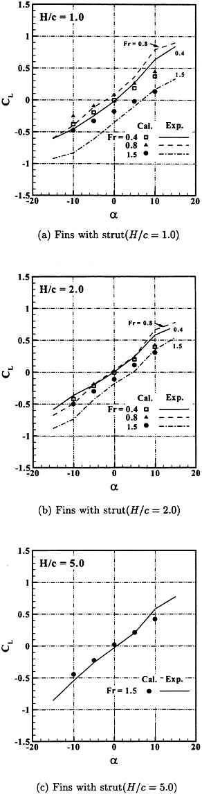
Fig. 9 Comparison of experimental results with computed results for CL versus α for fins attached to strut
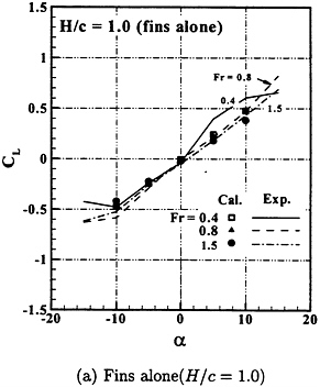
Fig. 10 Comparison of experimental results with computed results for CL versus α for fins alone
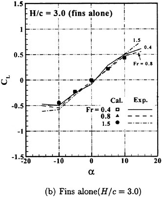
Fig. 10 Comparison of experimental results with computed results for CL versus α for fins alone
Fig. 11 shows the computed chordwise pressure distributions of the fins alone and also of the fins attached to the strut at Fr=0.8 for H/c=1.0 and α=5 degrees. The numerical results appear that the Kutta condition at the trailing edge both for the fins alone and the fins with strut is well satisfied. It can be seen that the present computational method with the linearised free surface condition can well predict the lift force of a submerged fin alone at submergnece of H/c≥1.0 where the non-linear free surface effect seems to be negligible.
Therefore, it can be understood that the discrepancy between the computed and measured values at the higher speeds of Fr=1.2 and 1.5 is attributed to the strong non-linear free surface effect by the strut, but not by the fin. This understanding could be also supported by the fact that the discrepancy in the two results decreases as the H/c increases and the free surface effect decreases. As the depth of submergence increases, the effect of the strut on the lift of the fins diminishes as can be deduced by comparing the results shown in Figs. 8 and 9. At the deepest submergence depth of H/c=5.0 as shown in Fig. 9c, CL curves for all Froude numbers in the present experiment almost converge to one curve; hence, as a representative one, the results for Fr=1.5 is presented. It appears evident from the present results that the consideration of the non-linear free surface effect for shallower depths of submergence in the numerical scheme would improve the computational results.
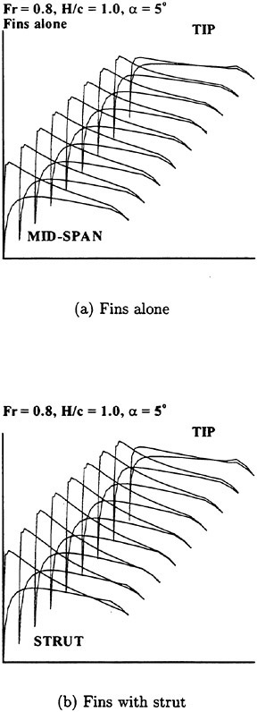
Fig. 11 Computed chordwise pressure coefficient distribution on the fin
In an unbounded fluid, it is commonly understood that the relation between the lift coefficient and the angle of attack for thin airfoils before the stall is linear. This fact is confirmed by the results shown in Fig. 10b for the fin-alone case at a relatively deep submergence of H/c=3.0. In addtion, this fact is
fins attached to the strut at a deeper submergnece of H/c=5.0.
However, when the fins are located close to the free surface, the behavior of CL seems to be represented, as indicated in Figs. 9a and 9b by an equation in the form of CL=C0+C1α. where C0 is a constant which depends upon the free-stream velocity and depth of subergence and C1 is a pure constant. The constant C0 whose value can be positive or negative depending on the free stream speed is the measure of the free-surface deformation created by the strut. The result shown in Figs. 9a and 9b are for the fins-alone case for H/c=1.0 and 3.0. Here, one can observe that the values of constant C0 seem significantly smaller (say, almost approaches to zero) than those for the case of fins with strut, indicating that the free-surface deformation generated by the fins is significantly smaller compared to that by the strut.
The effect of strut on the lift force is shown in Fig. 12 where ΔCL is obtained by subtracting the lift coefficient of fins alone from that of the fins attached to the strut. Since the strut effect is more prominent in shallow depth of submergence, the results are shown for H/c=1.0 and 2.0 for comparison. The computed results show a linearly decreasing trend with the increase of α while the experimental results do not exhibit any definite trend. The large discrepancies between the experimental and numerical results at the hightest speed of Fr=1.5 for H/c=1.0 can be judged due mainly to the nonlinear free surface effects as mentioned earlier.
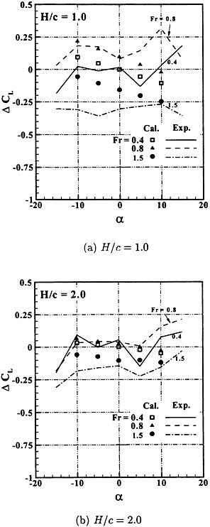
Fig. 12 Comparison of experimental results with computed results for strut effect on CL
From the wave-elevation results shown in Fig. 13, it can be deduced that the free surface deformation generated by the strut apparently changes the incidence angle of the free stream to the fins which changes with the free-stream velocity. In the present case, the strut-induced incidence angle of the flow tends to be positive for Fr=0.8 and negative for the higher Froude number s (Fr>1.0) as evidenced by the measured wave profiles shown in Fig. 13a where the strut is located between −0.5 and 0.5 in the x-coordinate. The CL shown in Fig. 6a supports the relation between the incidence angle created by the presence of the strut and CL. That is, for Fr=1.2 and H/c=1.0, CL>0, while at the greater Froude numbers CL<0.
The presence of fins at H/c=0.5 appears to alter the wave profile slightly as shownin Fig. 13b compared to the wave profiles in Fig. 13a. It can be observed in Fig. 13b that some ripples at Fr=0.4, reduction in the wave height and length at Fr=0.8, and more intensive wave breaking at the trailing edge of the strut at Fr=1.2. The wave profiles shown in Fig. 13c for the strut with fins for H/c=0.5, 0.8 and 1.0, α=0° and Fr=1.2 show very little changes. Fig. 13d shows the effect of the angle of attack on the wave profile. At α=10° the wave breaking occurs before the trailing edge(TE) of strut, while it occurs right at the TE at α=0°. Thus, the presence of fins at shallow depth of submergence with a moderate angle of attack at higher speeds can disturb the free surface significantly in the stern region of the strut.
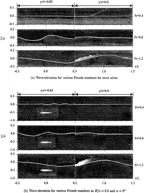
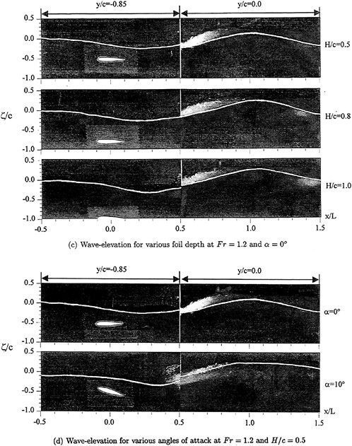
The effect of α on CL at H/c=0.5 and Fr=1.2 is manifested in Figs. 6a and 6b. The value of CL for α=0° from Fig. 6a is −0.4 while that for α=10° from Fig. 6b is about 0. One can deduce such results by observing the incidence angles of flow at the leading edge of the fins in Fig. 13d for α=0° and 10°.
Fig. 14 shows the computed and measured wave profiles at the fin mid-span plane (y/c=−0.85) for the strut alone and also for the strut with fins for α=0 degree at H/c=0.5 and 1.0. The strut is located between −0.5 and 0.5 in the x-coordinate. It can be clearly seen that the wave height due to the strut alone is slightly larger than that due to the strut with fins. For the case of the strut with the fins, the wave height for the shallow fin submergence of H/c=0.5 is smaller than that for the deeper submergence of H/c=1.0 due to the favorable wave interferences. This trend can be seen from the experimental results although the difference in the magnitude-is small.
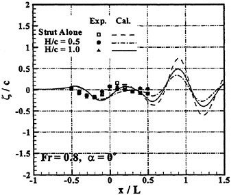
Fig. 14 Comparison of experimental and computational wave amplitudes (ζ/c) for strut alone and strut with fins at Fr=0.8
Fig. 15 shows the perspective wave patterns due to the strut with fins at Fr=0.8 for H/c=0.5 and 1.0 with α=0 degree. Although it is a little difficult to distinguish from the figure, the numerical results clearly show that the waves for H/c=1.0 case are, in general, larger than those for H/c=0.5 case. Fig. 16 shows the computed and measured wave profiles at the mid-span plane for the strut alone and also for the strut with fins at Fr=1.2. In general, the computed wave heights are larger than the experimental results.
The fins attached to the strut at α=0 dgree contribute to reduce the wave height compared with that for the strut alone, which is also observed in Figs. 13a and 13b. However, for the fins at α=10°, the numerical results show a reverse trend for the wave heights between H/c=0.5 and 1.0. Such a trend is also reflected in CL as shown in Fig. 6b.
The foregoing results clearly indicate that when the fins attached to a ship hull approaches near the free surface, they would definitely be influenced by the free surface deformation created by the advancement of the ship. Thus, the selection of the location of the control fins for a high-speed ship should be carefully determined by considering the ship-generated wave contour alongside of the ship.
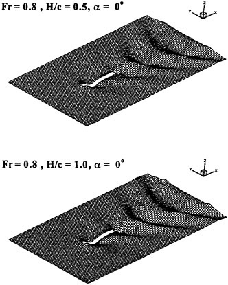
Fig. 15 3-D perpective wave patterns due to the strut with fins (computational results)
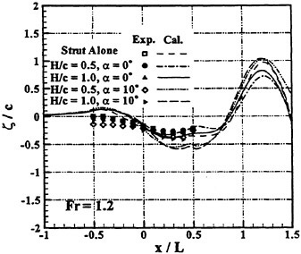
Fig. 16 Comparison of experimental and computational wave amplitudes (ζ/c) for strut alone and strut with fins at Fr=1.2
6. CONCLUSIONS
The free-surface effect on the lift characterisitcs of the fins attached to a body is found significant when the submergence depth of fins is less than three times the chord length. The dominant cause is due to the change in the flow incidence angle to the fins induced by the free-surface deformation caused by the strut. The wave elevations alongside the strut for the strut with the fins are lower than those of the strut alone. Therefore, the careful selection of the fin position to the body is necessary in view of lift and wave making resistance points.
The computational method based on the HOBEM appear to be useful in predicting the quantitative lift and flow characteristics of fin alone submerged at the depth of H/c≥1.0 and also of the fin attached to the strut up to moderately high speed even at a relatively shallow submergence. Further improvemnents of the computational scheme by taking into account the non-linear free surface effect will be necessary to upgrade the prediction capability for the fin performance near the free surface for high Froude numbers.
ACKNOWLEDGMENT
The first and the fourth author of this paper express their gratitudes for the supports of Korea Science and Engineering Foundation and Advanced Fluids Engineering Research Center of Pohang University of Science and Technology (POSTECH).
The assistance rendered by Messrs. Jae Ho Choi and Sung Jae Kim, who are the graduate students of POSTECH are greatly appreciated.
REFERENCES
1. Whicker, L.F. and Fehlner, L.F, “Free-Stream Characteristics of a Family of low Aspect-Ratio, All-Moveable Control Surface for Application to Ship Design,” DTMB Report 933, 1958, pp. 119.
2. Pitt, W.C., Nielsen, J.N. and Kaatari, G.E., “Lift and Center Pressure of Wing-Body-Tail Combinations at Subsonic, Transonic and Supersonic Speeds,” NACA Report 1307, 1959.
3. Wu, Υ.Τ., “A Theory for Hydrofoils of Finite Span,” Journal of Mathematics and Physics, Vol. 33, 1954, pp. 207–248.
4. Breslin, John P., “Application of Ship-Wave Theory to the Hydrofoil of Finite Span,” Journal of Ship Research, Vol. 1, No. 1, 1957, pp. 27–35.
5. Nishiyama, T., “Linearized Steady Theory of Fully Wetted Hydrofoils,” Advances in Hydroscience, Vol. 3, Academic Press Inc., Ν.Υ., 1983, pp. 237–342.
6. Nakatake, K. et al, “Calculation of the Hydrodynamic Forces Acting on a Hydrofoil,” Transactions of the West-Japan Society of Naval Architechs, No. 76, 1988.
7. Bai, K.J. and Lee, Η.Κ., “A Localized Finite-Element Method for Nonlinear Free-Surface Wave Problems,” Proc. of 19’th Symposium on Naval Hydrodynamics, 1992, pp. 113–130.
8. Ohmatsu, S. et al., “An Experimental Study on the Motion Control of Semi-Submerged Ships,” Journal of Soc. Naval Arch Japan, Vol. 152, 1983, pp. 229–238.
9. Mori, K.H. et al., “A Study on Semi-Submergible High Speed Ship with Wings-Its Resistance Characteristics and Possibility,” Naval Architecture and Ocean Engineering, Vol. 27, 1988, pp. 1–10.
10. Qi, X and Mori, K.H., “A Boundary Element Method for the Numerical Simulation of 3-D Nonli near Water Waves Created by a Submerged Lifting Body,” Journal of the Society of Naval Architects of Japan, Vol. 167, 1990, pp. 25–34.
11. Sclavounos, P.D. and Nakos, D.E., “Stability Analysis of Panel Methods for Free-Surface Flows with Forward Speed,” Proc. of 17th Symposium on Naval Hydrodynamics, The Hague, The Netherlands, 1988, pp. 173–193.
12. Boo, S.Y., “Application of Higher Order Boundary Element Method to Steady Ship Wave Problem and Time Domain Simulation of Nonlinear Gravity Waves,” Ph. D. disseration, Univ. of Texas, 1993.
13. Telles, J.C.F., “A Self-Adaptive Co-ordinate Transformation for Efficient Numerical Evaluation of General Boundary Element Integrals,” International Journal for Numerical Methods in Engineering, Vol. 24, 1987, pp. 959–973.
14. Lee, J.T., “A Potential-based Panel Method for the Analysis of Marine Propellers in Steady Flow,” Ph. D. Thesis, Department of Ocean Engineering, M.I.T., Cambridge, Mass, 1987.
15. Goldstein, R.J., “Fluid Mechanics Measurements,” Hemisphere Publications, 1983, pp. 630.
16. Lamb, H., “Hydrodynamics,” 6th Edition, Dover, 1932, pp. 738.
DISCUSSION
K.-h.Mori
Hiroshima University, Japan
Did you measure or compute drag force also? The relation between CL and CO is not so simple as in the unbounded case due to the free surface interaction. Sometimes the total drag is reduced. Especially the case where the lifting force is downward, negative, is interesting to the discusser.
AUTHORS’ REPLY
Thanks for your questions. No, we did not measure the drag force but we calculated the wave resistance. Since the content of the paper is too much, the results were not included. As you mentioned, the wave resistance of the strut with fins is varying depending on the speed and the incidence angle of the fin. As seen in the experimental and numerical results for the wave elevation in the paper, the wave elevations due to the strut with fins are lower than those of the strut alone and accordingly, it was found that the computed wave resistance decreased. However, it is presently not certain that the reduction in the wave resistance overweighs the change (possibly increase) in the viscous resistance due to the strut presence and then, resulting in the total drag reduction. It can be imagined that for a free model attached with fins, the lift force generated by the fins changes the draft and then, at certain speed range, the total drag can be reduced.
Numerical and Experimental Studies for the Prediction of Hydrodynamic Characteristics of Two-Dimensional Hydrofoils Operating Under the Free Surface
K.-S.Min, S.-H.Kang (Hyundai Heavy Industries Co., Ltd., Korea)
H.Streckwall (Hamburg Ship Model Basin, Germany)
ABSTRACT
Systematic studies have been performed for the prediction of hydrodynamic characteristics of 2-dimensional hydrofoils operating in the vicinity of free-surface. In this study, three numerical methods based on the potential theory, that is, vortex-lattice method, panel method and combined method have been developed. Among three methods, the vortex-lattice method always gives the closest results to the experimental measurements. From the practical view points, therefore, this method seems to be sufficient for 2-dimensional hydrofoils. In order to incorporate the geometric shape as much as possible and in order to extend the result to 3-dimensional cases, however, panel method has been tried with two different singulaity distributions on the free-surface. The numerical schemes could be well utilized to investigate the qualitative behavior of 2-dimensional hydrofoils operating in the vicinity of free-surface. However, they are not considered to be satisfactory yet to obtain sufficiently accurate quantitative information for actual design.
1. INTRODUCTION
In order to increase the ship speed significantly, it is necessary to prevent the rapid increase of the wave resistance. This purpose could be achieved by different ways. One way is to utilize the dynamic or static lift effects, and the other is to design the hull form of displacement type ships to be very fine. Hydrofoil boats together with the traditional planing hull ships are typical examples of dynamic effect ships, and the air cushion vehicle or the surface effect ships are those of the static effect ships.
On the other hand, the hull form of displacement type catamaran ships could be made very fine so as to achieve the goal of high speed by preventing rapid increase of wave resistance. In fact, catamaran ships have many practical advantages such as large deck area, high stability, superior maneuverability, easy operation and maintenance, etc. However, the most noticable merit is in the fact that ship size could be easily increased without any limitations and without sacrificing any other characteristics. The speed characteristics of high-speed catamaran ships could be significantly improved by properly combining the hull itself supported by buoyancy and the hydrofoil system which produces lift.
For hydrofoil boats or foil-catamaran ships, it is the common practice for the foil system to be operated in the vicinity of free-surface. There are two unavoidable problems due to the influences of free-surface. One is wave-resistance, and the other is the variation of hydrodynamic characteristics of the foil system. In other words, the lift and drag characteristics of the foil system are changed as it approaches to free-surface. However, no theoretical method has been developed yet to predict the change of characteristics according to the submergence of foil system with sufficient accuracy for the utilization of actual design. Therefore, the authors have made their long theoretical and experimental studies not only to prepare the prediction method for the variation of lift and drag according to the depth of foil
system from the free-surface with sufficient practical accuracy, but also to develop new section shapes to be utilized for propeller blade or foil sections with superior performance characteristics to that of the existing sections.
Originally, study for 2-D foil was initiated as the preliminary study for the extension to 3-D foil. However, it has been recognized that 2-D foils are more important and efficient than 3-D foils for foil-catamaran ships. It is considered that the vortex-lattice method is the best for 2-D foils in the practical view points such as simplicity and accuracy. In order to reflect the foil geometry more accurately (particularly thickness effect) and in order to extend to 3-D foils, however, the panel method has been developed also. In this paper, results on the 2-D foil study shall be summarized from the authors’ general studies for the estimation of hydrodynamic characteristics of hydrofoils operated in the vicinity of free-surface.
2. BASIC THEORY
A moving foil with constant speed in deep water produces constant lift. At the same time, constant drag force is acting on the foil. The drag is generated mainly due to viscosity of the fluid and the pressure distribution around the foil. However, lift and drag are changing as the foil approaches to free-surface, that is, the lift is generally decreased and wave-resistance in addition to two drag components mentioned above is produced due to generation of wave. The technique to analyze the flow-characteristics of a real fluid around a moving foil in the vicinity of free-surface has not been sufficiently developed yet. Furthermore, there is no definite idea how longer it would take to improve the technique to the level of practical applications. Therefore, the authors have decided to treat this foil problem by the potential based numerical method neglecting viscosity. Fortunately, the influence of viscosity on the lift is small and the method is expected to be useful to estimate the generated lift. For the practical estimation of drag, however, the effect of viscosity should be estimated by proper methods and combined with the result by potential theory. The theoretical and experimental method for the estimation of viscosity effect on the drag has also been developed.
2.1 Potential treatment
First, it has been assumed that the fluid is non-viscous and incompressible, and the fluid motion is irrotational. The coordinate system as shown in Figure 1 has been introduced to represent the fluid motion around a foil, and it has been assumed that the coordinate system is moving with the foil.
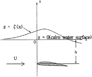
Fig. 1 Coordinate system
When the free-surface and the velocity potential are denoted by ζ and ![]() the governing equation is as follows:
the governing equation is as follows:
(1)
The kinematic boundary condition and the dynamic boundary condition are as follows:
(2)
(3)
In equation (3), g and U denote gravitational acceleration and moving speed of the foil, respectively. The boundary conditions (2) and (3) could be combined into one equation for the velocity potential ![]() as follows:
as follows:
(4)
From the free-surface boundary condition represented by equation (4) and the boundary condition on the foil surface, solution for the velocity potential ![]() could be obtained by the numerical methods discussed in the next chapter. Once velocity potential
could be obtained by the numerical methods discussed in the next chapter. Once velocity potential ![]() is obtained, lift and potential drag (induced drag) as well as free-surface deflection could be found. In 2-D theory, lift and potential drag could be determined by various different methods. In order to treat the problem based on the physical phenomenon and in order to extend the method to 3-D problem, however, the pressure
is obtained, lift and potential drag (induced drag) as well as free-surface deflection could be found. In 2-D theory, lift and potential drag could be determined by various different methods. In order to treat the problem based on the physical phenomenon and in order to extend the method to 3-D problem, however, the pressure
integration method has been adopted as follows:
(5)
In equation (5), Ρ is the pressure acting on the foil surface found from Bernoulli theorem and ![]() is the unit normal inward vector on the foil surface. Then, the lift and the potential drag are found as follows:
is the unit normal inward vector on the foil surface. Then, the lift and the potential drag are found as follows:
(6)
(7)
The deflection of free-surface, that is, the form of wave could be found from the equation (3) as follows:
(8)
2.2 Viscous correction for the Drag
In order to estimate the overall drag, it is necessary to estimate the viscosity effect on the drag by proper methods. To do this, the authors have adopted the form factor concept assuming two main parts from the viscous effect, that is, frictional drag and form drag. The concept could be expressed as follows:
(9)
Where, DV, DF, DFM and k represent viscous drag, frictional drag, form drag and the form factor of the foil, respectively. The frictional drag is calculated as follows:
(10)
Where, ρ, CF and ℓ represent density of water, frictional drag coefficient and circumferential length of the foil. The frictional drag coefficient is found from the ITTC Standard correlation line as follows:
(11)
(12)
Where, RN, c and ν represent Reynolds Number, chord length of the foil and kinematic viscosity of the fluid.
The authors have tried to express the form factor in the following form:
(13)
Where, a1, and a2 are unknown coefficients to be determined and t is the thickness ratio of the foil in fraction of chord length. The unknown coefficients, a1 and a2, were first estimated by the power law of boundary layer theory [1] and modified later reflecting the experimental results. In this way, the viscous drag is estimated. Finally, the overall drag is estimated by combining the potential drag and the viscous drag as follow:
(14)
3. NUMERICAL METHOD
The key point of the numerical method is how to represent the foil and the free-surface by distributing singularities. The mode of singularity distribution determines the speed of convergence as well as the convergence itself. The authors have tried numerous types of singularity distributions to investigate the proper representation of foil and free-surface as well as quick convergence. Among them, three typical methods shall be discussed.
3.1 Method 1
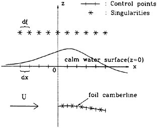
Fig. 2 Coordinate System and Singularity Distributions for the Method 1
In the first method, point sources and point vortices have been distributed on the camberline of the foil to simulate the thickness effect of the
foil and to generate lift. In order to derive the streamline which represent the deflection of free-surface, that is, the wave profile, point sources have been distributed at some constant distance above the calm water surface. Figure 2 schematically shows this arrangement.
In order to find the exact potential ![]() from the exact nonlinear free-surface boundary condition (4), the exact position of the free-surface ζ should be known. However, there is no way to find the free-surface position in the beginning. Therefore, the authors have utilized the following iterative procedure. Assuming that the approximate solutions Φ and z′ of the exact potential
from the exact nonlinear free-surface boundary condition (4), the exact position of the free-surface ζ should be known. However, there is no way to find the free-surface position in the beginning. Therefore, the authors have utilized the following iterative procedure. Assuming that the approximate solutions Φ and z′ of the exact potential ![]() and the free-surface ζ are known, express
and the free-surface ζ are known, express ![]() as follows:
as follows:
(15)
In equation (15), φ is the correction for the approximate potential Φ. If equation (15) is substituted into equation (4), the following expression is obtained:
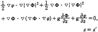
(16)
In order to set up the linear system from the equation (16), calculation points have been set up on the approximate free-surface z=z′ and on the camberine of the foil. By solving the linear system for the strength of sources and vortices, the approximate potential Φ has been up-to-dated progressively. The wave profile has been continuously revised from the equation (3) as follows:
(17)
In equation (17), Φ is the potential for the previous solution z′old.
3.2 Method 2
In the second method, the actual shape of the foil has been divided into numerous panels with the distribution of constant strength dipoles and sources. Point sources have been distributed at some constant height from the calm water surface to derive the wave profile as adopted in the Method 1. Figure 3 schematically shows this arrangement. Therefore, the method is the combination of the panel method for the foil and the point source method for the free-surface.
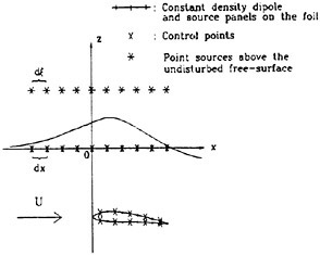
Fig. 3 Coordinate System and Singularity Distributions for the Method 2
Among the overall potentials, those for the foil itself have been obtained by Green’s theorem as follows:
(18)
If the source strength in equation (18) is assumed to be equal to the normal derivative of undisturbed potential, then the equation (18) becomes integral equation for the perturbation potential. The steps for the actual numerical solution is as follows:
-
express the perturbation potential
 as in the Method 1, that is, as in equation (15)
 -
set-sup the simultaneous equations from equation (16) and (18)
-
solve the linear system iteratively
The remaining steps are the same as those in the Method 1.
3.3 Method 3
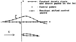
Fig. 4 Coordinate System and Singularity Distributions for the Method 3
The third method is the pure panel method.
As was done in Method 2, the foil surface has been divided into numerous panels with the distribution of constant strength dipoles and sources. Dipole and source panels with constant strength have been distributed on the undisturbed free-surface. Figure 4 schematically shows this arrangement.
In Method 3, Green’s theorem for the foil and the free-surface is as follows:
(19)
The source strength for the foil in equation (19) is assumed to be equal to the normal derivative of undisturbed potential. To handle the source strength for the free-surface in equation (19), the following relation from the free-surface boundary condition has been utilized:
(20)
The equation (19), then, becomes the integral equation for the perturbation potential and the remaining procedures for the solution is the same as those in Method 2.
4. EXPERIMENTAL STUDY
As well-known, the simulation of 2-dimensionality for the test of 2-D foils operated in the vicinity of free-surface is very difficult. In general, cavitation tunnels are useless for this purpose. Therefore, it was decided to conduct the tests in the deep-water towing tank. To do this, so-called 2-D walls with several different sizes were manufactured using aluminium plates. Special 3-component balance has also been designed and manufactured with the capability of depth and angle of attack adjustments. 2-D wall and sketch of 3-component balance are shown in Figures 5 and 6. Tests were carried out in the towing tanks of HMRT* and HSVA** independently. However, details of the experimental studies shall not be discussed here. Figure 5 shows the actual 2-D foil tests.
|
* |
Hyundai Maritime Research Institute |
|
** |
Hamburgische Schiffbau Versuchsanstalt (Hamburg Ship Model Basin) |
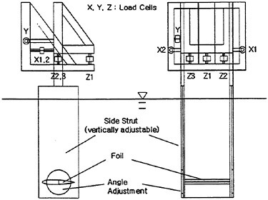
Fig. 5 Sketch of the three component balance
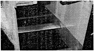
Fig. 6 Typical 2-dimensional foil test
5. INTRODUCTION OF HMRI NP-SERIES SECTION
As an effort to develop new section shapes superior to existing ones, the authors have devised numerous different sections and analyzed their hydrodynamic characteristics including pressure distributions around the foils. Finally, the new section shape has been invented and named HMRI NP-Section [2]. The section shape has been described in Figure 7.
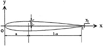
Fig. 7 Description of HMRI NP-Series Section
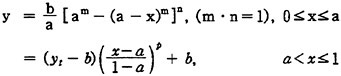
(21)
In equation (21), various symbols represent the
followings:
a=distance from the nose to the position of the maximum thickness
b=half maximum thickness
n=form exponent of the leading part
p=form exponent of the trailing part
yt=half tail thickness
The section shape is described by very simple equations, yet its hydrodynamic characteristics are superior. The section shape has been patented from four countries (Korea, Japan, Germany and Netherland).
6. TYPICAL RESULTS AND COMPARISON
In the course of developing numerical schemes, calculations were performed for more than 100 foils and for various operational conditions. Among them, two typical cases—one from NACA 66-sections [3] and one from HMRI NP-sections—were selected to examine the result of calculation and to compare them with the results of experiment. Table 1 shows the results of calculations and experimental measurements for NACA 66–009–4 foil for various depth ratios and various angles of attack. This foil represents the foil of NACA 66-series thickness form with 9% thickness combined with NACA 0.8-a meanline with 4% camber ratio.
Table 1 Theoretical Estimation and Experimental Measurement of Hydrodynamic Characteristics for NACA 66–009–4 (0.8-a Meanline) Foil
−FN=3.5
|
Depth Ratio (h/C) |
a (deg.) |
CL |
10×CD |
||||||
|
MI |
M2 |
M3 |
Exp* |
MI |
M2 |
M3 |
Exp* |
||
|
0.4 |
−2.0 |
0.12 |
0.16 |
0.17 |
0.17 |
0.18 |
0.15 |
0.15 |
0.15 |
|
0.0 |
0.25 |
0.30 |
0.31 |
0.27 |
0.17 |
0.18 |
0.16 |
0.17 |
|
|
2.0 |
0.38 |
0.43 |
0.45 |
0.39 |
0.18 |
0.22 |
0.20 |
0.22 |
|
|
4.0 |
0.51 |
0.55 |
0.59 |
0.49 |
0.21 |
0.27 |
0.24 |
0.31 |
|
|
1.0 |
−2.0 |
0.17 |
0.21 |
0.23 |
0.18 |
0.18 |
0.15 |
0.15 |
0.20 |
|
0.0 |
0.34 |
0.38 |
0.40 |
0.31 |
0.18 |
0.19 |
0.19 |
0.19 |
|
|
2.0 |
0.49 |
0.52 |
0.56 |
0.45 |
0.21 |
0.22 |
0.23 |
0.26 |
|
|
4.0 |
0.63 |
0.68 |
0.73 |
0.57 |
0.25 |
0.32 |
0.28 |
0.37 |
|
|
2.0 |
−2.0 |
0.18 |
0.22 |
0.24 |
0.20 |
0.20 |
0.16 |
0.15 |
0.18 |
|
0.0 |
0.36 |
0.40 |
0.42 |
0.34 |
0.18 |
0.20 |
0.19 |
0.20 |
|
|
2.0 |
0.53 |
0.57 |
0.61 |
0.49 |
0.20 |
0.22 |
0.23 |
0.26 |
|
|
4.0 |
0.70 |
0.73 |
0.78 |
0.64 |
0.25 |
0.32 |
0.28 |
0.38 |
|
|
4.0 |
−2.0 |
0.19 |
0.23 |
0.25 |
0.20 |
0.18 |
0.15 |
0.15 |
0.18 |
|
0.0 |
0.38 |
0.42 |
0.44 |
0.35 |
0.17 |
0.19 |
0.18 |
0.20 |
|
|
2.0 |
0.57 |
0.60 |
0.63 |
0.51 |
0.18 |
0.24 |
0.22 |
0.26 |
|
|
4.0 |
0.75 |
0.79 |
0.82 |
0.68 |
0.22 |
0.30 |
0.27 |
0.37 |
|
|
* Mean value of 3 different measurements |
|||||||||
Table 2 shows the results of calculations and experimental measurements for HMRI NP-009–4 foil for various depth ratios and various angles of attack. This foil represents the foil of HMRI NP-series thickness form with 9% thickness described in equation (21) combined with circular arc camber with 4% camber ratio. Figures 8 and 9 show the variations in lift and drag according to foil depth and the comparisons between numerical calculations and experimental measurements for HMRI NP-009–4 foil.
Table 2 Theoretical Estimation and Experimental Measurement of Hydrodynamic Characteristics for HMRI NP-009–4 (Circular arc camber) Foil
−FN=3.5
|
Depth Ratio (h/C) |
a (deg.) |
CL |
10×CD |
||||||
|
MI |
M2 |
M3 |
Exp* |
MI |
M2 |
M3 |
Exp* |
||
|
0.4 |
−2.0 |
0.14 |
0.16 |
0.18 |
0.16 |
0.13 |
0.12 |
0.12 |
0.13 |
|
0.0 |
0.28 |
0.31 |
0.32 |
0.27 |
0.14 |
0.15 |
0.13 |
0.15 |
|
|
2.0 |
0.41 |
0.44 |
0.46 |
0.38 |
0.18 |
0.19 |
0.17 |
0.20 |
|
|
4.0 |
0.54 |
0.56 |
0.59 |
0.49 |
0.25 |
0.22 |
0.21 |
0.28 |
|
|
1.0 |
−2.0 |
0.19 |
0.21 |
0.24 |
0.18 |
0.14 |
0.14 |
0.12 |
0.14 |
|
0.0 |
0.36 |
0.38 |
0.40 |
0.32 |
0.15 |
0.18 |
0.16 |
0.17 |
|
|
2.0 |
0.51 |
0.53 |
0.57 |
0.45 |
0.21 |
0.23 |
0.20 |
0.24 |
|
|
4.0 |
0.66 |
0.69 |
0.73 |
0.57 |
0.31 |
0.30 |
0.25 |
0.33 |
|
|
2.0 |
−2.0 |
0.20 |
0.22 |
0.24 |
0.18 |
0.14 |
0.14 |
0.12 |
0.16 |
|
0.0 |
0.37 |
0.41 |
0.43 |
0.34 |
0.15 |
0.18 |
0.16 |
0.18 |
|
|
2.0 |
0.55 |
0.57 |
0.61 |
0.49 |
0.21 |
0.23 |
0.20 |
0.24 |
|
|
4.0 |
0.72 |
0.74 |
0.79 |
0.64 |
0.31 |
0.30 |
0.26 |
0.35 |
|
|
4.0 |
−2.0 |
0.22 |
0.23 |
0.25 |
0.20 |
0.14 |
0.14 |
0.12 |
0.16 |
|
0.0 |
0.40 |
0.43 |
0.44 |
0.37 |
0.14 |
0.16 |
0.14 |
0.18 |
|
|
2.0 |
0.59 |
0.61 |
0.64 |
0.52 |
0.18 |
0.22 |
0.18 |
0.24 |
|
|
4.0 |
0.78 |
0.80 |
0.83 |
0.69 |
0.28 |
0.27 |
0.23 |
0.33 |
|
|
* Mean value of 3 different measurements |
|||||||||
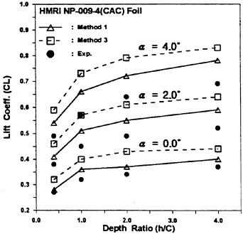
Fig. 8 Variation of Lift according to Foil Depth
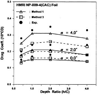
Fig. 9 Variation of Drag according to Foil Depth
7. DIDCUSSIONS AND CONCLUSIONS
The authors have long performed systematic studies for the prediction of hydrodynamic characteristics of 2-D foils operated under the free-surface. As a part of such efforts, the authors have tried numerous different numerical schemes based on the potential theory, and three typical methods have been presented and discussed in this paper together with very limited experimental studies. Among three numerical methods, the method 1 (vortex-lattice method) always gives the closest results to the experimental measurements, while the results by the method 3 (pure panel method) always show the biggest differences from those of experiment. All of three methods tend to overpredict the lift and underpredict the drag. In the actual computations, it is sufficient to distribute 50 singularities on the foil camberline and 100 in the free-surface to obtain practically complete convergence, and even over 95% of complete convergence could be obtained by the singularity distributions of 10 on the foil camberline and 20 in the free-surface in the Method 1. In the Method 3, however, more than 50 panels on the foil surface and 100 panels in the free-surface are required to have 95% of complete convergence. Therefore, computation is much more complicated and takes much more time by the Method 3 than by the Method 1. The Method 2 is in the middle of the Method 1 and the Method 3 in every sense. From the practical view points, therefore, the vortex-lattice method is the best in terms of accuracy, simplicity, etc.
The three numerical methods tried by the authors could be well utilized to investigate the qualitative behavior of 2-D foils operated in the vicinity of free-surface. However, they are not considered to be satisfactory to abtain sufficiently accurate quantitative information for actual design. Ultimately, direct solution method of Nervier-Stokes equation for the real fluid should be developed. However, this technique is in its early stage nowadays and no definite idea is available how long it would take to improve the technique to the level of practical application. There exists pesimistic view that such days would never come.
For the practical design, the authors are utilizing the result of regression analysis for the test results of series foils [4]. At this moment, this is the most convenient, accurate and practical way for the prediction of foil characteristics. The weak point of this method is in the fact that the method is applicable only to a certain type of series foils. It is the authors’ hope and desire that a practically sufficient rational method for the prediction of hydrodynamic characteristics of foils operated under the free-surface could be prepared in the near future. After then, study on the interference phenomenon between ship hull and foil system should be performed.
REFERENCES
1. Schlichiting, H., “Boundary-Layer Theory”, McGraw-Hill Book Company, 6th Ed., 1968.
2. Min, K-S. and Lee, H-G., “Systematic Studies on the Development and the Estimation of Hydrodynamic Characteristics of New Hydrofoil Sections Moving under the Free Surface”, Technical Report No. HMRI-95–06–S100, Hyundai Heavy Ind. Co. Ltd., June, 1995.
3. Brockett, T., “Minimum Pressure Envelopes for Modified NACA-66 Sections with NACA a=0.8 Camber and Buships Type I and Type II Sections”, NSRDC Report 1780, Feb. 1966.
4. Min, K-S. and Kang, S-H., “Systematic Studies on the Estimation of hydrodynamic Characteristics of 2-Dimensional Hydrfoils Moving under the Free Surface”, the Proc. of the Spring Meeting, 1996 of the Society of Naval Architects of Korea, April, 1996.
DISCUSSION
G.Jensen
Hamburg Ship Model Basin, Germany
I would like to congratulate the authors for their extensive work on the hydrodynamics of submerged hydrofoils. The great value of the paper results from the combination of experimental and numerical results.
You have investigated several singularity schemes to compute the 2-d potential flow. Concerning the descretization of the hydrofoil you find that you get better agreement with the measurements with the vortex lattice methods than with the panel method. This result is surprising on first glance because the panel method describes the shape of section accurately, while the vortex lattice is arranged on the camber line, with some crude correction for the thickness effect. This result is, however, in line with corresponding application of these methods to propeller flows. It is known, however, that the application of boundary layer theory in combination with the panel method gives good results in that case. I believe that the errors due to missing thickness and missing viscous effects somehow cancel in the vortex lattice scheme. Therefore I recommend using the panel method in combination with boundary layer theory in this case as well.
After this basic theory is well established now, I consider it necessary to extend the theoretical investigations to the 3-dimensional problem, to instationary effects like in a seaway and to the cavitation problem. What are your plans in this respect?
AUTHORS’ REPLY
Thank you very much for the valuable comments and suggestions from Dr. Jensen of HSVA. I would like to make the following general replies.
This study was initiated as the basis of developing the theoretical prediction method of hydrodynamic characteristics for 3-dimensional hydrofoils operated in the vicinity of free-surface. However, it has been recognized that the 2-D case is practically more important than the 3-D case and effort has been concentrated on the 2-D study, because our main purpose is designing a hydrofoil system for the super high-speed foil catamarans. In this case, the hydrofoil system is much closer to the 2-D condition than to the 3-D condition.
One may think that the panel method is better than the vortex-lattice method, since it describes the section shape more accurately. In my view, however, it is virtual, but not real. Both methods are approximate. None is exact. Through my long and extensive studies, I have an impression that the mechanism of lift generation by vortex distribution is simpler and better than that by dipole distribution.
Theoretical predictions of propeller performance for the steady state by both the potential-based vortex-lattice method and panel method agree well with experimental results for the design condition (generally lightly loaded condition). For the 2-D foil with free-surface, however, there are too many differences in performance characteristics between numerical predictions and experimental results. I have long wondered why. It seems that the 2-D foil problem is much simpler than the propeller problem.
Another study has also been performed to develop a direct solution method by Navier-Stokes equation for the real fluid. At this moment, it works for the Reynolds Number (RN) range of up to 105. For the actual utilization, it should be capable of handling the case with RN greater than 107. What is bothering me is that this method does not produce quantitatively useful results according to our limited comparison with experiment and that I have no idea how long it will take to be practically useful.
We are now trying to establish the direction of future study. We would like to significantly improve the computational accuracy for the 2-D case first. After that, we will start the 3-D study immediately.
DISCUSSION
H.H.Chun
Pusan National University, Korea
The discusser appreciates the authors’ efforts in developing a practically sufficient rational method for the prediction of hydrodynamic characteristics of foils operated under the free surface. Also, a high compliment should be paid for the achievement in developing new foil section shapes which can be described by simple equations, but hydrodynamic characteristics are superior.
As far as the lift is concerned, it has been known that the potential theory can predict well the lift force of a foil in unbounded flow and also at a comparatively deep submergence depth from the free surface. At a depth ratio (h/C) of 4.0 which can be assumed to be unbounded flow, the deviation between the experimental results and the computational results seems to be big and the deviation becomes bigger as the angle of attack increases, as shown in Fig. 8. In view of this, have the authors checked the accuracy of the codes by comparing the computational results with the known experimental results such as pressure distribution and wave elevation? Conducting the 2-D experiment is very complicated and hard; therefore have you compared the experimental results conducted by HMRI and HSVA? How much is the difference between the two results?
Lastly, the discusser would like to ask the authors to open the comprehensive experimental data of the new foils which can be valuably used not only for the validation of the computational results, but also for the design of foils operating in the vicinity of the free surface.
AUTHORS’ REPLY
Many thanks for the valuable comments and suggestions from Prof. Chun. I would like to reply as follows:
The numerical lift calculation for the foils in the unbounded fluid gives very close results to some known exact potential solutions (about 5% less). If free-surface boundary condition is imposed from the beginning, however, the difference becomes bigger even if the foil submergence is comparatively deep from the free surface. This is one of the areas to be investigated further.
In real flow, separation and stall phenomena occur as angle of attack increases. However, such phenomena have not been reflected in the present scheme. The flow is assumed to be perfectly attached regardless of the angle of attack. It is the authors’ opinion for the reason why difference increases with the increased angle of attack.
In fact, 2-D experiments are very difficult and experimental results are not considered to be sufficiently accurate. Major series experiments were conducted three times with some time intervals. Each time, the measurements were significantly different. The maximum difference between experiments is about 30% from the same model basin, and a similar amount of difference occurs between model basins, i.e., between HSVA and HMRI. The impression from the actual foil design and full-scale ship sea trial is that experiment underpredicts and numerical computation overpredicts the lift. It is the tentative conclusion that the real value is in between.
The authors are planning to publish the date book incorporating the theoretical and experimental studies similar to the “Theory of Wing Sections” for the NACA foil sections.
Study on the Mechanism of Resistance Reduction by Means of Micro-Bubble Sheet and on Applicability of the Method to Full-Scale Ship
Y.Yoshida,1 Y.Takahashi,1 H.Kato,2 O.Watanabe1
(1Ishikawajima-Harima Heavy Industries Co., Ltd., Japan, 2University of Tokyo, Japan)
ABSTRACT
In order to study the applicability of skin friction reduction by micro-bubbles to actual ships, the authors propose a mathematical model for the mechanism of skin friction reduction, which they verify through experiment.
The proposed model for bubbly two-phase flow satisfactorily elucidates flow phenomena observed in experiment, and leads to a practical method for estimating skin friction on a bubble-covered wall. Further, the model proves to adequately treat bubbly flow in boundary layers of widely differing scale. The model promises to be applicable to deriving a quantitative expression of the scale effect between model and full-scale unit regarding the behavior of bubbly flow and the resulting frictional resistance.
An example is given of predicting the resistance of a bubble-covered full-scale ship, based on an evaluation of the balance between the energies additionally consumed for bubble air injection and economized through resistance reduction.
NOMENCLATURE
NOTE: Other symbols not listed here are defined in the text at the positions where they appear.
|
a, b |
proportional constants |
|
Β |
law of wall constant |
|
c |
empirical coefficient |
|
CF |
averaged frictional coefficient |
|
Cf |
local frictional coefficient |
|
db |
diameter of bubble [m] |
|
DR |
resistance reduction ratio |
|
f |
offset of hull surface from z-axis [m] |
|
g |
gravitational acceleration [m/s2] |
|
jx, jy |
flux [m/s] |
|
K |
form factor of ship |
|
K0, K1 |
parameters determining the profile of void fraction defined by Eqs. (80) (81) |
|
k |
turbulent energy [m2/s2] |
|
lb |
mean free path of bubble [m] |
|
lm |
mixing length [m] |
|
mA |
added mass of bubble [kg] |
|
P |
pressure [Pa] |
|
QG |
air supply rate [l/min, m3/min] |
|
qg |
buoyancy-induced bubble rise velocity [m/s] |
|
q′(i) |
amplitude of turbulence velocity at ith time increment [m/s] |
|
R |
resistance [N] |
|
r |
total resistance coefficient of ship |
|
rf0 |
frictional resistance coefficient of ship |
|
rw |
wave-making resistance coefficient of ship |
|
T* |
integral time scale [s] |
|
U |
reference velocity [m/s] |
|
Uτ |
friction velocity [m/s] |
|
|
time-averaged velocities [m/s] |
|
u′, v′ w′ |
turbulence velocities [m/s] |
|
V |
volume of a bubble [m3] |
|
VR |
velocity difference between bubble and liquid [m/s] |
|
x, y, z |
Cartesian coordinates [m] |
|
X, Y, Z |
bubble displacement [m] |
|
α |
local void fraction |
|
αav |
average void fraction in boundary layer |
|
β |
bubble-induced upward stream velocity [m/s] |
|
δ |
boundary layer thickness [m] |
|
∈ |
turbulent energy dissipation [m2/s3] |
|
κ |
von Kármán constant |
|
μ |
viscosity [Pa·s] |
|
ν |
kinematic viscosity [m2/s] |
|
ρ |
density [kg/m3] |
|
τ |
shear stress [N/m2] |
|
τm |
increase of turbulent stress [N/m2] |
|
τt |
reduction of turbulent stress [N/m2] |
|
|
velocity potential [m2/s] |
|
ω |
angular frequency of liquid phase turbulence [rad/s] |
|
∇ |
immersed volume of ship [m3] |
SUBSCRIPTS AND DIACRITICAL MARK
|
b |
variable concerning bubble |
|
G |
gas |
|
L |
liquid |
|
m |
mean variable |
|
w |
variable close to wall |
|
0 |
without bubbles |
|
1 |
with bubbles |
|
2 |
change from variable without bubbles |
|
ˆ |
root mean square |
INTRODUCTION
Viscous Frictional Resistace of Hull
Reduction of hull frictional resistance will contribute to reducing the power required for ship propulsion, and consequently to lowering the emission from machinery of CO2 gas, which is pointed out to be one of the harmful gases that add to the global greenhouse effect.
Hull resistance comprises viscous and wavemaking components, of which the viscous component further comprises viscous friction and viscous pressure resistance.
Of the above components, wave-making and viscous pressure resistances are largely determined by the hull form, in respect of which minimization of resistance has been to date consistently sought for given sets of design conditions through tests on models in laboratory basin and through parallel theoretical calculations. As a result, hull forms have today attained a level of improvement such that further very significant lowering of the above-cited resistances can no longer be anticipated.
Such considerations on hull resistance lead us to look for a breakthrough in the reduction of the only remaining component, which is viscous frictional resistance. This form of resistance constitutes more than 75% of the total hull resistance in the case of very large crude oil carriers, so that its reduction should contribute significantly to diminishing the load on propulsive machinery. Similar circumstances apply, if to a lesser extent, also to ships of faster speed.
Despite the foregoing circumstances, the fact that viscous frictional resistance is largely determined by the Reynolds number and the area of wetted hull surface has hitherto deterred endeavors to derive means of significantly lowering this form of resistance. The development of such a means can thus be considered to constitute one of the few promising aspects still retaining room for improvement in the field of naval hydrodynamics.
The present study approaches this subject with a proposal to reduce the frictional resistance of a turbulent boundary layer through the injection of a micro-bubble sheet.
Reduction of Frictional Resistance by Means of Micro-Bubble Sheet
The method proposed of reducing frictional resistance consists of injecting a sheet of micro-bubbles measuring not more than 1 mm in diameter into a turbulent boundary layer flowing at velocities between several m/s and over 10 m/s. Water and air, respectively, are normally envisaged for the liquid and gas phases.
The arrangement for realizing the concept is illustrated in Fig. 1.
An experiment relevant to the above concept has been performed by McCormick et al. [1]. They substantiated the effect of resistance reduction obtainable with this method through measurements made of the resistance upon generating bubbles by electrolysis on the surface of an axisymmetric streamlined body. The reduction of resistance was 10–30%, but the energy consumed in electrolysis will have largely offset this gain. What merits attention, however, is the discovery that frictional resistance is reduced by the injection of a bubble sheet into the layers of flow close to the wall.
The bubbles need not have to be generated by electrolysis, and later studies have adopted a simpler method of blowing air bubbles into the flowing stream through a porous plate, in the manner illustrated below for the case of wall formed by ceiling.
Bogdevich et al. [2] laid a flat porous plate face upward on the floor (lower wall) of a cavitation tunnel to let air bubbles blow out of the holes of the plate. Measurements were made of the shear stress sustained by the wall (floor) and the transverse distribution of void fraction across the flow. A ratio of resistance reduction amounting up to 80% was obtained at some positions, but the fact that the void fraction rose locally up to 80%—exceeding the maximum replenishment ratio of 74% for spherical inclusions—leaves doubt as to whether the flow in the layers close to wall had still presented a true form of bubbly liquid.
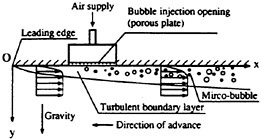
Fig. 1 Sectional view of arrangement for frictional resistance reduction by means of micro-bubble injection
The Bogdevich report contains measured data arranged by Reynolds number, by rate of air supply, and by void fraction, and further discusses the effect of each of these factors. No mention, however, is made of the form presented by the flow streaming along the wall.
Madavan et al. [3] used a cavitation tunnel of 508 mm×714 mm cross section and 762 mm length, on the ceiling and floor of which porous bubble-injecting plates were set, and the shear stress exerted on wall was measured. The porous plates were provided with holes alternatively of 0.5 μm and 100 μm diameter, and the speed of water flow was varied in the range between 4.6 m/s and 16.8 m/s. Resistance reduction of up to 80% was recorded. It was noted that the resistance reduction ratio tended to deteriorate with displacement downstream.
Madavan et al. have also presented the results of theoretical examination [4]. They reasoned from the theoretical and empirical equations given by Einstein and Sibree that the mean viscosity should rise with increasing void fraction. This can be likened to the increase of consistency seen when raw cream is whipped to absorb air bubbles. Applying the theory of mixing length, the frictional resistance was derived by substituting the density and the viscosity of a single-phase flow with the space-averaged mean density and viscosity of bubbly flow.
Marié [5], similarly to Madavan, adopted the concept of mean viscosity, to propose a convenient model in which the viscous layer varied its thickness upon injection of bubble sheet.
Now, Einstein’s theoretical equation should more correctly be applied to treating liquids dispersed with bubbles of size smaller than considered here, i.e. of the order of fine suspensions (0.01 μm–100 μm particle diameter). This leaves some doubt as to whether Einstein’s theory can validly be applied to the present case of bubbles measuring up to 1 mm. Other shortcomings that can be noted in the analysis of Madavan and Marié include the absence of consideration on the kinetic properties of bubbles, and of regard to scale effect.
Kato et al. [6] used a TE type cavitation tunnel (350 mm long, 50 mm wide and 100 mm high) equipped with slit on ceiling (upper wall) and on floor (lower wall), from which a sheet of water mixed with air bubbles was injected. Their data are arranged according to frictional resistance reduction ratio. The same authors [7] further examined the difference in effect obtained with bubbles injected from upper and lower walls of the channel.
Guin et al. [8] used a two-dimensional channel (100 mm wide, 10 mm high), for which they devised a sampling void fraction meter for determining the distribution of void fraction generated by the micro-bubbles. Measurements made using this meter were compared with corresponding data obtained with the conventional optical fiber instrument. They derived a valid void fraction distribution across flow, which indicated the frictional resistance reduction to be predominantly governed by the void fraction in the layers close to wall.
At the Research Institute of Ishikawajima-Harima Heavy Industries [9], tests were conducted in laboratory basin using a flat-bottomed model hull (40 m long, 600 mm breadth, 50 mm draft), with air bubbles injected from hull bottom alternatively at bow and amidship. The model was moved at speeds between 5 m/s and 7 m/s, and data were acquired on frictional resistance reduction along the full hull length of 40 m. The friction reducing effect, while lowering with displacement downstream, could still be discerned at hull stern, 40 m downstream of bubble injection point.
In what follows, a discussion will be presented on a calculating procedure focused on consideration of the orders of magnitude (scale) of the values being treated, to derive a theoretical basis for approximate treatment of data, adopting as a paremeter the scale of the envisaged variable.
ASSUMPTIONS ADOPTED
Overall Perspective
We will here deal with a two-dimensional flow streaming along a flat wall.
We adopt a concept we call ‘linear configuration distribution’ which means the distribution of void fraction across flow cross section approximated by a straight line. The validity of the approximation will be verified by comparison with experimental data.
The first step of analysis will be to set forth assumptions for deriving practical and convenient equations that will explain the qualitative tendencies presented by the physical phenomena, with the objective of clarifying the dependence of data on the parameters that are adopted.
When treating flows of high Reynolds number, the resulting small length scale of vortexes necessitates adopting some form of turbulence model. The theory of two-dimensional turbulent boundary layer making use of mixing length is a classical approach dating back to Prandtl’s work of 1933 [10], but which is still today often used for roughly estimating the frictional resistance of single-phase flow, and in the present instance the theory should serve reasonably as a starting point for analyzing bubbly flow.
In the case of single-phase flow, the shear stress applying on the wall and the distribution of flow velocity across the flow both depend largely on the Reynolds’ stress. Considering the occurrence close to wall of the phenomenon known as ejection, which is a form of turbulent flow structure that governs Reynolds stress, and whose thickness does not reach even one tenth of that of the boundary layer, the reasonable approach to deriving the basic equations should be to concentrate on expressing the changes to turbulence brought by the motion of bubbles close to the wall, rather than on the spatial variation of mean density across the entire cross section of boundary layer, as determined by the quantity of bubbles present in the layer.
Based on the above consideration, we here assume the master equations to be a system of equations deriving from the formulation of phenomena occurring in a layer adjoining the wall of a thickness
comparable to the bubble diameter. This assumption is also based on the observation noted by Guin et al. [11] that the mean void fraction is determined by that in the immediate vicinity of wall.
The change in turbulence is governed by promotive and suppressive factors [12]: The former promotive factors include (a) the wake flow generated when the bubble changes its form from spherical shape (note: No such wake is generated when the bubble retains spherical shape, the flow being devoid of vortexes), and (b) modification to momentum accompanying inflow of liquid of volume equal to that of a bubble that has been displaced. The opposite suppressive factors include (a) bubble resistance arising from the difference in velocities between gas and liquid phases, and (b) dissipation of turbulent energy accompanying change in volume or shape.
Tsuji et al. [13] reports noting that, upon pouring particles into a vertical flow of air, reducing the particle size tended to suppress turbulence. Gore [14], upon rearranging available experimental data, discovered that turbulence tended to be suppressed when the particle diameter became smaller than the integral turbulence scale.
Based on the above empirical observations of Tsuji and Gore, we will here assume that, when suppression of turbulence is observed, bubble diameter should be significantly smaller than the length scale of turbulence, and that the bubbles should retain their spherical shape. This assumption contains the corollary that, in such case of turbulence suppression, no vortexes should be seen around the bubbles, and that the flow can be considered tantamount to a uniform stream carrying with it solid spherules. Consequently, the dominant factor that suppresses turbulence should then be bubble resistance arising from the difference in flow velocity between the gas and liquid phases.
Basic and Constituent Equations
To simplify our discussion, we assume a constant flow of incompressible fluid. We adopt as basic equation that which governs the boundary layer, and which comprises within it the conservation laws of momentum and mass. We adopt the mathematical coordinate system shown in Fig. 1.
Bubbles injected from ceiling (upper wall), tend to concentrate in layers close to wall. Taking time-averaged values, while the bubbles are subjected to buoyancy, their movement is constrained by the wall, and the bubbles, after flowing some distance after their injection into stream and collecting in the layers close to the wall, settle down to flow along the stream creating a void fraction that gradually lowers with displacement downstream.
The time-averaged laws of momentum and mass conservation are expressed on a model of homogeneous flow as follows:
(1)
(2)
Applying the theory of mixing length, the expression giving the shear force exerted on wall, which constitutes one of the structural equations, becomes:
(3)
Forces Acting on Bubble
The forces acting on a bubble are: (a) resistance deriving from parallel motion, (b) added momentum force, (c) hysteresis force, (d) force deriving from pressure gradient, or else buoyancy. Additionally, lift is exerted in a field where shear is present, as in the case of a boundary layer.
As regards added momentum force, added mass is here assumed to equal half the mass of water occupying the same volume as the displaced bubbles. Hysteresis force [15] is of integrated form, and is generally neglected for convenience of calculation, and since in a bubbly flow, in particular, it is considered to be small, the neglect of hysteresis force can be considered not to be of any consequence.
In respect of lift, a well-known study is that of Saffman [16] for the case of minute solid spherules in a liquid flow presenting small shear, with small difference in flow velocities between liquid and solid phases. Gas bubbles, however, are subject to change of void shape—be it only to a small extent—which can result in the force being exerted in direction opposite to that of Saffman’s lift, depending on the conditions governing the flow [17]. Unfortunately, there is available today no method of treating lift in a flow field involving shear, and in the present instance, we will ignore the effect of lift, assuming the bubbles to be amply small in size to justify the neglect.
We will further neglect the force deriving from pressure gradient—apart from buoyancy.
The resistance of bubble ascribable to parallel movement depends on the impurity of liquid. Tomiyama et al. [18] classified impurity into three levels, and indicated resistance coefficients corresponding to each level. According to their classification, normal city water would correspond to ‘medium impure’ and ‘highly impure’ water. Their ‘pure’ water is what is obtained upon triple distillation of city water.
Assuming normally-used water to fall under the category of ‘medium impure’ and ‘highly impure’ water, flow of such water containing micro-bubbles of amply small size can be conveniently treated for deriving frictional resistance using Stokes’ formula:
(4)
SHEAR STRESS ACTING ON WALL
Frequency Response
Given the value of void fraction, we will seek
to derive the shear stress acting on wall. As already mentioned, we assume the time-averaged flow velocities not to differ between gas and liquid phases. Also, for the time being, we will not consider buoyancy, which is a constant external force. We will take this force into account when later we derive the master equation for void fraction distribution.
The mathematical model we adopt is shown in Fig. 2.
A bubble injected into a turbulent boundary layer will respond in its motion to the turbulent flow velocity of the liquid phase. The density of air being about 1/103 of that of water, the momentum force of air can be neglected in comparison with the added momentum of displacing liquid. This added momentum will have the effect of retarding the response of bubble motion in relation to the liquid phase velocity, to result in a difference of velocity between the two phases. This velocity difference will generate resistance in the bubble, and reaction force in the adjoining liquid.
Calculation of the velocity difference between liquid and gas phases calls for knowledge of the kinetic characteristics of bubble motion, so we will proceed by considering the equation of motion.
In Fig. 2, we place the origin at the point where a gas particle is positioned in time-averaged displacement in a flow traveling along the straight line AA drawn at a distance from the wall.
The equations of motion governing the relative displacement in the directions x and y, respectively parallel and normal to the direction of flow, are
(5)
(6)
Fourier transformation is applied to the above Eqs. (5) and (6), to derive the amplitude ratio of x in reference to ![]() and of y in reference to
and of y in reference to ![]() the results of which are defined as GX and GY:
the results of which are defined as GX and GY:
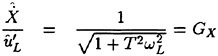
(7)
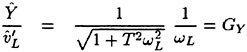
(8)
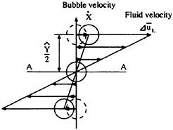
Fig. 2 Mathematical model for considering shear force on wall
The bubble presents a time constant
(9)
In what follows, we will adopt the root mean square as the representative value for the variables contained in equations. For instance, in the case of the resistance force ΔRv acting on bubble,
(10)
In particular reference to the term (1−GX)GY,
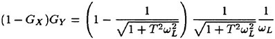
(11)
In the discussions to follow, we will distinguish three ranges of bubble motion frequency classified according to the order of magnitude of the time constant Τ and of that of the turbulence period 2π/ωL:
(12)
(13)
(14)
We will designate the above three ranges of frequency as ‘low’, ‘medium’ and ‘high’ frequency ranges.
The medium frequency range defined by Eq. (13) corresponds to the case where an accurate answer is considered, strictly based on the given assumptions, and the treatment in such cases generally becomes most complex. The derivation could be simplified to some extent through such expedients as expansion into series in cases where a predominant frequency is already known, but we will in this instance forego proceeding to such treatment.
The other two frequency ranges are susceptible to simplification of the constituent equations, and the dependency on parameters can be expected to be more easily made clear.
High-frequency Range
We will here consider the case defined by Eq. (14). In this case, from Eqs. (9) and (11),
(15)
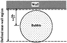
Fig. 3 Definition of region immediately adjoining wall (ceiling)
which, upon substituting into Eq. (10), gives
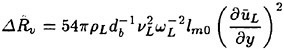
(16)
where lm0 is used instead of ![]() .
.
The region immediately adjoining the wall (ceiling) is, as illustrated in Fig. 3, limited to a layer of thickness equal to the bubble diameter, with y=db/2 adopted as representative position of bubble.
The mixing length in this region is
(17)
and incorporating the representative bubble position defined above,
(18)
Considering the turbulence period 2π/ωL to equal the time scale T*L of turbulence representing that required for a vortex to pass over a given point in space,
(19)
Substituting Eqs. (18) and (19) into Eq. (16),

(20)
Since the average length along wall occupied by a spatial element of bubble is (π/6α)1/2db,
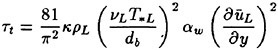
(21)
Shear stress is subject not only to suppressive but also to promotive factor, such as caused by momentum exchange. When a bubble displaces, the space it leaves behind it is filled by an equal volume of water, which brings with it displacement of momentum. This movement of bubble in the turbulent boundary layer is tantamount to an equal volume of water being set in motion. The mechanism of additional stress generation is equal to the Reynolds stress generated by liquid particle motion, so that the added shear element
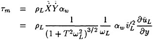
(22)
Considering the high-frequency range we are treating here,
(23)
Equation (23) for τm, representing the promotive element of shear stress, contains a term of magnitude ![]() and since from Eq. (14), ΤωL≫1 in the high-frequency range considered here, τm is negligibly small in this range. Since Eq. (21) representing the suppressive element does not have any term containing ΤωL, it means that, in this high-frequency range, the predominant factor governing shear stress is that which suppresses rather than promotes shear stress.
and since from Eq. (14), ΤωL≫1 in the high-frequency range considered here, τm is negligibly small in this range. Since Eq. (21) representing the suppressive element does not have any term containing ΤωL, it means that, in this high-frequency range, the predominant factor governing shear stress is that which suppresses rather than promotes shear stress.
The change in shear stress can be considered to derive from the shortening of mean mixing length lmb of bubble in a turbulent field. In Eq. (3), the second term representing vortical viscosity (Reynolds stress) is predominantly greater than the first term for molecular viscosity, so that
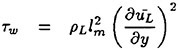
(24)
(25)
(26)
(27)
Hence, the shear stress reduction can be expressed by
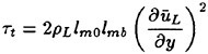
(28)
By comparing Eq. (21) with Eq. (28), we derive
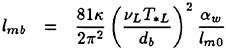
(29)
(30)
The product of turbulent time scale T*L and the root mean square of turbulence velocity ![]() i.e., represents a value that is 1/2 of the mean free path (dimension of length) so that this product can be considered to be proportional to the mixing length.
i.e., represents a value that is 1/2 of the mean free path (dimension of length) so that this product can be considered to be proportional to the mixing length.
In particular, in a region where the universal logarithmic law is applicable, the following relation holds:
(31)
that is,
(32)
The value νL/Uτ indicated between parentheses represents the length scale of viscous sublayer.
Substituting Eq. (32) into Eq. (30),
(33)
Representing by the letter a the proportional constant in the above expression
(34)
where
(35)
It is indicated from the form presented by Eq. (34) that the effect of the presence of bubbles can be expressed by modification brought to the von Kármán constant:
(36)
(37)
(38)
(39)
In Eq. (38), lm represents the mathematically modified mixing length.
The logarithmic law can continue to be applied, and such application will not conflict with Eq. (32).
The modification to be applied to the von Kármán constant is, from Eqs. (34) and (37),
(40)
The modified mean von Kármán constant is, from Eq. (39),
(41)
(42)
An interesting fact brought to light upon examining Eq. (42) is that the fraction given between parentheses, i.e. the turbulence suppressing parameter, has the numerator representing the viscous sublayer and the denominator proportional to the bubble length, both numerator and denominator being in the scale of length. The length of viscous sublayer being closely related to the turbulence scale according to Eq. (32), the present model can be considered to constitute a mathematical model indicating that the ratio between turbulence and bubble length serves as parameter to represent the suppressive factor of turbulence. This corroborates the empirical finding that the turbulence is suppressed when the bubble size is small relative to the degree of turbulence expressed in length scale.
Low-frequency Range
In this case, from Eq. (12), ΤωL≪1, so that, Eq. (23) for the shear stress promoting factor τm containing ![]() in the denominator comes to acquire a predominantly high value:
in the denominator comes to acquire a predominantly high value:
(43)
Friction Resistance
We will here seek in asymptotic approximation the skin friction ratio Cf/Cf0 between cases of bubble presence and absence for the high-frequency range, where the shear stress suppressive element is predominant.
Frictional resistance coefficient can also be derived by simultaneously seeking the basic and structural equations, but we will here seek the solution by adopting the universal logarithmic law.
In the absence of bubble, where the universal logarithmic law holds,
(44)
(45)
(46)
(47)
In the presence of bubbles, using the modified mean von Kármán constant κ1,
(48)
(49)
(50)
(51)
In Eqs. (44) and (48), assuming the boundary layer to have the same thickness (in dimensional unit) whether in the presence or absence of bubble, replacing y with δ,
(52)
(53)
where
(54)
(55)
The subtraction Eq. (53)–Eq. (52) gives
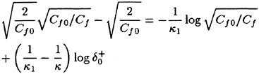
(56)
Expanding Eq. (56) in the vicinity of ![]()
![]() and discarding the terms other than linear,
and discarding the terms other than linear,
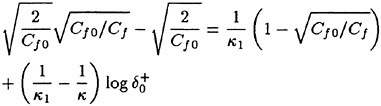
(57)
Since
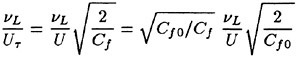
(58)
substituting Eq. (58) into Eq. (40), and the result into Eq. (42), and further into Eq. (57), the final solution becomes
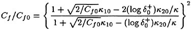
(59)
where
(60)
(61)
(62)
The conditions governing a micro-bubble differ from those of a suspension of minute particles in a dispersive medium, and in Eq. (62), and we have let νL=ν as an approximation.
In Eq. (59) Cf was nondimensionalized by reference to ![]() (Eq. (55)): If the same Cf of Eq. (59) is nondimensionalized by reference to
(Eq. (55)): If the same Cf of Eq. (59) is nondimensionalized by reference to ![]() instead of
instead of ![]() as in the case of Cf0 (Eq. (54)), Eq. (59) becomes
as in the case of Cf0 (Eq. (54)), Eq. (59) becomes
(63)
We have thus derived an expression that is extremely easy to compute.
So far, we have considered frictional resistance in the high-frequency range of bubble motion, that is in the range ΤωL≫1 as defined by Eq. (14), to derive Eq. (63) as analytical solution (asymptotic solution). In this range, Cf/Cf0 decreases monotonically with increasing [turbulence-length scale]/[bubble diameter]—i.e. increasing effect of bubble. We have also seen in an earlier section that the shear force promotive element τm is in this range far smaller than the opposite suppressive element τt. In other ranges the stress promotive element τm can no longer be neglected, and in the low-frequency range, it is this shear-promotive element that becomes predominant.
In other words, what the present mathematical model indicates as tendency is that, in the high-frequency range, the bubble motion responds only weakly to external force, and consequently undergoes only small movement, with resulting small exchange of momentum between the two phases, and this enhances the effect of shear stress suppression by bubble resistance. Conversely, in the low-frequency range, the bubble motion response is sharp, with consequent active interface momentum exchange and attendant enhancement of shear promotive effect.
The three ranges of bubble motion frequency are roughly related to the classification of bubble size and of the skin friction ratio Cf/Cf0 as schematized in Fig. 4.
The shaded domain marked “present region” is the high-frequency region treated in what precedes.
VOID FRACTION
We now take up the treatment of αw, the void fraction in the layers close to wall, which is the variable inputted into Eqs. (42) and (63), and of that of the bubble diameter db contained in Eq. (42).
With regard to bubble diameter, examination of a cross section of the flow fields indicates that bubble size is not uniform, but is distributed through a wide range [12], to make it difficult to determine uniquely. Moreover, a definitive means of measuring bubble diameter still remains to be developed.
Such considerations lead us to doubt whether it is a practically valid approach to assume the bubble diameter to be known, and to derive therefrom the distribution of void fraction, and based on the resulting data to calculate Cf/Cf0.
To overcome this difficulty, we consider the procedure of setting as simultaneous equations the master equation of void fraction distribution and Eq. (42) relating the mean von Kármán constant to bubble size and thereby to eliminate the bubble diameter db and the proportional constant a, thus to substitute bubble diameter with the void fraction distribution.
As elements that govern bubble diffusion, we will simplify our consideration by taking into account solely turbulence and buoyancy.
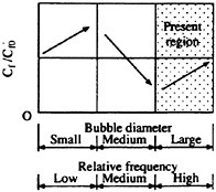
Fig. 4 Perturbational classification
In such case, bubble velocity will be determined uniquely by resistance force. Adopting Stokes resistance for this force, it will be proportional to velocity, so that when considering bubble motion, it is no longer necessary to solve the equation of motion based on force, and this permits deriving the velocity by simply superposing the different velocity elements.
Treating a bubble as diffusive particle, the gas phase is considered as a continuous fluid constituted of such diffusive particles. The mathematical model of the diffusive particles is shown in Fig. 5.
The law of mass conservation applicable to a stream flowing through the boundary ABCD, expressed in terms of the fluxes jx and jy is
(64)
A diffusing gas phase of void fraction α conveyed by the mean velocity of the streaming water and by buoyancy can be approximated by
(65)
(66)
Where c is an empirical coefficient that possesses the physical meaning of diffusion coefficient.
The second term of Eq. (65) represents the flux induced by the turbulence velocities generated by the diffusive particles (2) and (4) in Fig. 5.
Before substituting Eqs. (65) and (66) into Eq. (64), we define the prior conditions of:
(67)
(68)
(69)
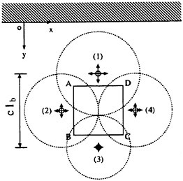
Fig. 5 Mathematical model of flow field
The above terms have been approximated to zero to indicate that, after substitution, they are negligibly small in comparison with the other terms.
Having adopted the above conditions, substitution of Eqs. (65) and (66) into (64) gives
(70)
The fact that the flux in y-direction must become zero at the wall yields the relation
(71)
which, upon expansion, becomes
(72)
We consider the above Eq. (72) to represent the master equation of void fraction distribution. The same equation is validly applicable to a two-dimensional channel.
The first and second terms written within parentheses in Eq. (72) can be considered to represent the diffusion of bubble that is due respectively to the liquid phase turbulence and to the void gradient.
To seek the mixing length lb of the gas phase, we only need to reexamine the bubble equation of motion. In the layers close to the wall where the universal logarithmic law is applicable, the gas phase mixing length lb and the actual (i.e. not the mean) liquid phase mixing length lm0 are related to each other by
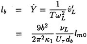
(73)
(74)
In determining the void fraction, for convenience of calculation, the liquid phase mixing length is expressed in the form
(75)
In a domain where the universal logarithmic law is applicable,
(76)
(77)
Obtaining lb from Eqs. (74) (75), and substituting Eq. (76) and (77) into Eq. (72), further arrangement results in
(78)
Equation (78) is a separable-variable differential equation and is thus easily solved:
(79)
where
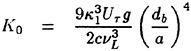
(80)
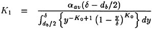
(81)
In Eqs. (80) and (81), K0 and K1 are parameters that determine the shape of the void ratio distribution, with K0 indicating the position of void peak, and K1 the magnitude of the void fraction as a whole.
In Fig. 6, the void fraction distribution is seen to present three distinct patterns for the cases of K0<1, K0=1, K0>1: In the case of K0>1, the void fraction diverges toward wall (ceiling). When K0=1, the void distribution does not diverge, but rises linearly to reach maximum value at wall, and represents the case where the mean turbulence is the most suppressed, and consequently the kinetic energy is minimized. The potential energy of buoyancy also is smaller than when K0<1, so that this case can be considered to present the most stable pattern of void fraction distribution.
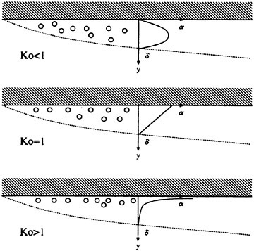
Fig. 6 Patterns of void fraction distribution
From Eq. (80), it is seen that the value of K0 varies with the 4th power of bubble diameter, and is thus extremely sensitive to change in bubble size. From the same Eq. (80), the proportional constant a also sensitively affects K0, so that uniquely determining the bubble size which is in actuality widely distributed, and to input such a value in a system of equations in order to estimate the pattern of void fraction distribution must be considered an almost impossible proposition.
We will hence seek the converse approach mentioned earlier of identifying the void fraction characteristics by fitting to measurement the theoretical Eq. (79), through manipulation of K0 and K1. With the resulting value of K0, we determine db/a using Eq. (80), setting it simultaneously with Eq. (63) and constitute a series of equations in two-way coupling in terms of Cf/Cf0.
A simple one-way coupling could also be constituted by substituting Uτ by Uτ0 and κ1 by κ in Eq. (80).
The procedure of calculation is schematized in Fig. 7.
SUBSTANTIATION OF THEORY
We will substantiate the foregoing theory by corroboration with three series of experimental data presenting different scales of flow field [8] [19] [9]. The three flow fields are schematized in Fig. 8.
In matching the master equation (72) for void fraction to data from experiment, the key constant requiring to be adjusted is the coefficient c of this equation.
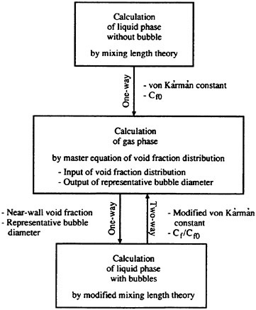
Fig. 7 Procedure of calculation
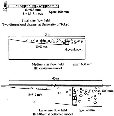
Fig. 8 Flow field of experiments for substantiation of theory
It ultimately proved that, on all the three scale of corroboration referred to above, a value of 0.01 for the coefficient c provided the best fit of calculated curves to experimental data.
Small Flow Field (Two-dimendional channel of University of Tokyo)
The experiment that is cited [8] has been performed on a two-dimensional channel with bubble injected from ceiling. Conducted at flow speeds close to those of actual ship (5–8 m/s) for average void fractions below 7%, the local void fraction was almost zero at channel center, and increased roughly linearly with approach toward wall (ceiling), (see Fig. 9).
This pattern of void fraction distribution corresponds to the case of K0=1 in Fig. 6.
If the linear pattern of void fraction distribution could be consistently adapted without sacrificing the estimating accuracy, even if limited in the range of applicability, the principle should still prove useful in practical application.
We now proceed to calculation applying the two-way coupling method and the measured values of void fraction in the layers close to wall, as well as a simplified one-way coupling procedure adopting the approximation of linear void fraction distribution (K0=1 in Fig. 6), followed by an examination of the respective ranges of applicability.
The results of calculation are presented in Fig. 10, relating the skin friction ratio Cf/Cf0 to mean void fraction. The calculation was performed by adjusting Eqs. (80) and (81) in such manner as to fit to the measured void fraction distribution the calculated curves relating α/αav to displacement from wall.
The plots indicated by triangles are the results obtained with two-way coupling method, the results of simplified one-way coupling method being indicated by the square plots. The open circles represent data measured by Guin [8]. Also drawn in for reference are Madavan’s data [3], as well as calculated results using Marié’s theory [5].
The agreement in trend shown between the calculated curves and measured plots in Fig. 10 can be considered to substantiate the validity of the present model. The appreciable deviation from calculation shown by the open circle plots in the range beyond 0.05 mean void fraction can be ascribed to the fact that, whereas Cf/Cf0 in Guin’s measurement has been normalized to Um0 of void fraction at channel axis in the absence of bubble, the calculation has, for convenience, had Cf normalized to the main stream velocity in bubble presence, and Cf0 to that in bubble absence, and this expedient can affect the accuracy of calculation, particularly in
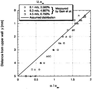
Fig. 9 Void fraction in 2D channel
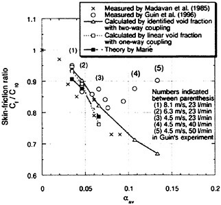
Fig. 10 Skin-friction ratio in 2D channel
channels of narrow width.
This leaves room for further study to devise a method for more accurately estimating the main stream velocity in calculations on bubble flow.
In respect of the simplified calculation by one-way coupling method, the square plots of Fig. 10 would indicate mean void fraction αav=0.05 as the limit of applicability of this method.
In the case of a very large flow field, treated further on, the measured mean void fraction marked an inordinately high value of 0.06 when the stream velocity=7 m/s, the air injection rate 300 l/min and the measuring point x=3 m (position of sensor mounted nearest bow). Taken as a whole, however, the mean void fraction was much smaller, so that, as a general rule, the simplified method using one-way coupling should ensure adequate accuracy. In this case, the mean void fraction αw in the layers close to wall can be substituted by the mean void fraction across the boundary layer, αav
(82)
Medium Flow Field (IHI cavitation tunnel)
The data cited [19] are from tests performed in a tunnel of 600 mm×600 mm cross section, with air bubbles injected through a slit of 5 mm width and 150 mm span located on tunnel upper wall. Measurements were made along 3 m of channel length, with stream flowing at 8 m/s.
Substantiating examination was, also in this case of large flow field, performed using one-way coupling calculation, assuming K0=1 or linear void fraction distribution.
Test data are plotted in Fig. 11, in terms of measured Cf/Cf0 against displacement downstream from a virtual origin.
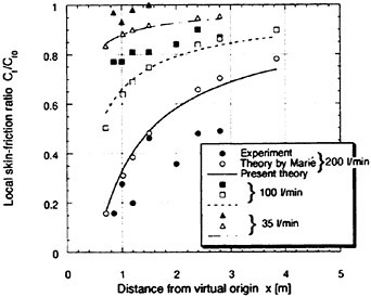
Fig. 11 Local skin-friction ratio obtained in IHI cavitation tunnel
The deviation of measured plots from calculation toward the virtual origin for the runs at lower stream velocities can be ascribed to a portion of the bubbles straying out of the boundary layer immediately following injection from slit. Otherwise, the calculated curves may be considered to acceptably express the overall trend of measured plots.
Large flow field (IHI 40 m long flat-bottomed model in basin test [9])
The results are presented in Fig. 12, where the data from calculation and measurement are compared. The data can be considered to indicate calculation adequately representing the effect of differences in air supply rate.
Comparison with Conventional Theory.
For making comparison, Figs. 10, 11 and 12 are also drawn with plots indicating data calculated on Marié’s theory. The theory has given agreement with experiment on a level with the present theory in the case of Figs. 10 and 11, but in the case of Fig. 12, the present theory has proved to yield data presenting trends with far greater qualitative correspondence.
The better performance of the present theory can be attributed to the fact that it has taken account of the effect of relative velocity between liquid and gas phases, i.e. the frequency response to change in the degree of turbulent flow by change in stream velocity, which was not considered in Marié’s theory.
Methods applying the mean viscosity, including that of Marié, have hitherto been considered to yield estimates well agreeing with experiment, but for cases where the values are sensitively affected by differences in stream velocity and where the field of flow is large, the present theory should be considered to have brought improvement.
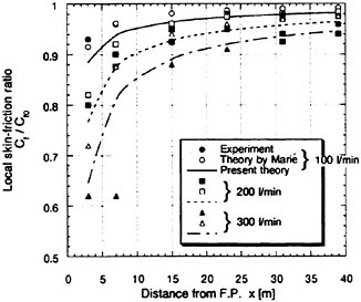
Fig. 12 Local skin-friction ratio obtained on IHI 40 m long flat-bottomed model
Particularly in the case of large flow fields, improvement of agreement with measured data should contribute to enhancing the expressibility of scale effect, and this should be of special interest to designers of systems in shipbuilding and marine engineering.
PRELIMINARY ESTIMATION OF THE GAIN OF PROPULSIVE POWER OF FULL-SCALE SHIP
Viscous Frictional Resistance
Applying the basic theoretical considerations treated earlier in this report, we will in what follows consider the skin friction exerted on hull surface.
In ship design, a widely-practiced procedure for roughly estimating skin friction in the absence of bubbles is to substitute the hull by a plate of equal wetted surface area, and to apply a classical two-dimensional equation for resistance estimation, such as that proposed by Schoenherr.
We here adopt the same approach, to consider the problem locally in two dimensions, and further neglect the effect on skin friction ratio Cf/Cf0 brought by the presence of radius of curvature in the longitudinal direction of hull girth. Provided, however, that in treating the local skin friction Cf0 when devoid of bubble serving as reference value, considering its vital influence on subsequent calculations, phenomena will be treated locally, to apply the CFD code [20] for calculations on flow field around hull in the absence of bubbles.
As regards the void fraction αw in the layers close to wall, we assume its distribution in normal direction to the hull surface to be linear, as assumed in the preceding calculations for comparison with data from experiment. Then, from Eq. (82), αw becomes equal to twice αav, the mean void fraction across the boundary layer.
Calculation of Bubble Trajectory for Mean Void Fraction Across Boundary Layer on Hull Surface
Even adopting the assumption of linear void fraction distribution across boundary layer, we must still solve the equation of motion of bubble, and derive the void fraction distribution in direction normal to hull surface. We will in what follows describe this procedure.
As equation of motion, we add to Eqs. (5) and (6) the expression to account for the diffusion term deriving from the time-averaged velocity for buoyancy. We obtain the tree-dimensional formula
(83)
(84)
(85)
for the coordinate system shown in Fig. 13.
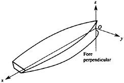
Fig. 13 Coordinate system for ship hull
Change of stream velocity in the x-direction will be neglected, since the void fraction can be considered determined solely by bubble diffusion in the remaining y- and z-directions.
As regards bubble volume, Boyle’s law will be applied, with bubble diameter assumed to change with volume:
(86)
Only quasi-static change of volume with pressure will be taken up for consideration.
The velocity of turbulence is expressed by
(87)
(88)
where ar is distribution ratio of turbulence velocity in radial direction, θ indicates the direction of diffusion.
The velocity of turbulence is not isotropic. In this instance, we assume in approximation that while anisotropic individually in the x- and y-directions, it is isotropic in the radial direction, and we calculate ar by referring to Laufer’s experimental data [21], the results of which are cited in Table 1. In the table, r indicates distance from the hull surface.
Table 1 Distribution ratio of turbulence velocity
|
τ/δ |
ar |
|
0.1 |
0.461 |
|
0.2 |
0.559 |
|
0.3 |
0.646 |
|
0.4 |
0.664 |
|
0.5 |
0.671 |
|
0.6 |
0.684 |
|
0.7 |
0.714 |
|
0.8 |
0.735 |
|
0.9 |
0.750 |
|
1.0 |
0.750 |
Turbulence Velocity
We apply the Markov process model [19] in order to obtain ![]() , which prescribes that the probability of a datum being created at a given instant is influenced by the corresponding probability governing the datum of one step earlier.
, which prescribes that the probability of a datum being created at a given instant is influenced by the corresponding probability governing the datum of one step earlier.
The energy of liquid turbulence kL and its rate of dissipation ∈ are assumed to be those determined by CFD calculation.
Preliminary Verification of Bubble Trajectory Calculation Program
For the purpose of verifying our bubble trajectory calculating program, bubbles were injected from the wetted surface of a model hull to acquire data on bubble trajectory.
The experimental equipment was of such arrangement as to let the bubble sheet issue from side plate at bow, to be entrained for some distance downstream then descend beneath hull bottom and rise again at stern. The principal specifications of the model are: LBP=7 m, B=1.08 m, d=0.261 m. The observed data on this complex trajectory was compared with calculation on trajectory calculating program as shown in Fig. 14.
In Fig. 14, the observed bubble trajectory is superposed on calculated data, for ship speed varied in steps from 2.2 to 3.5 m/s, with bubble diameter estimated to be 0.75 mm from photograph of bubble taken on a field close to bubble injection opening.
Agreement is seen for the position at which the bubbles start to disappear beneath hull bottom. The agreement, however is not good for the position of bubble reappearance from hull bottom.
The discrepancy can be ascribed to the actual bubbles tending to agglomerate during displacement downstream, and thus to become larger than when it was flowing further upstream.
The calculated trajectories reveal fluctuating movement in vertical direction, which can be ascribed to turbulence affecting the calculated results, but the amplitude of fluctuation is not large.
Bubble diffusion in direction tangential to hull surface cannot be said to have been fully substantiated, but the fact that bubble fluctuation was small, as indicated above, would justify the surmise that, in cases where the influence of upward flow
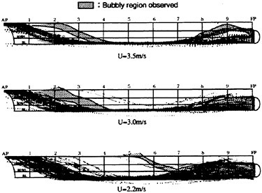
Fig. 14 Observed trajectories of bubble sheet superposed on calculated configurations
component is relatively small, the void fraction generated by bubble sheet injected from hull can be estimated in fair approximation by the present method.
Wave-making Resistance (modified thin ship theory)
In a model hull, the injection of bubble is said to little affect the wave-making resistance [22], but it remains to be examined whether the same applies also to the case of full-scale ship. Particularly in the case where the bubbles are injected from hull side, the main stream can be expected to acquire a form similar to bubble plume, so that the effect of differences in hull form should require examination.
In view of the above observation, we will apply the theory of potential flow to the case of bubbly flow, to examine how the distribution of singular points characterizing hull form would be affected by the presence of bubbles, and seek how the question might best be treated on full-scale ship.
We adopt a coordinate system as shown in Fig. 15. In the absence of bubble, the main stream would solely have a horizontal component U.
Estimation of Propulsive Power Gain.
Letting (βx, βy, βz), represent the added mainstream velocity brought by the bubble-induced upward flow, the kinetic and dynamic conditions governing the stream are
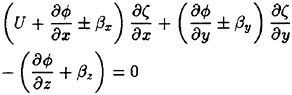
(89)
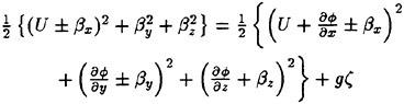
(90)
on z=ζ (wave height).
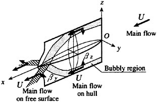
Fig. 15 Double model coordinate system with main stream flowing on both sides of hull above and below free surface
Assuming the bubbles to rise toward free surface in layers along the hull side, we let the upward and horizontal components of the stream assume the orders of magnitude given by
(91)
(92)
The above free surface conditions are the same as for bubble-absent case. The velocity potential is
(93)
where S0 is the projection of y=f(x, z) onto y=0 surface.
Equation (93) indicates that the hull center surface is distributed with bubble-injection openings of strength
(94)
The second term of Eq. (94) represents the effect of upward flow component.
The foregoing treatment leads to the conclusion that, on a wall-sided hull surface, the change brought to wave-making resistance is zero. On a full-scale ship, if bubble size can be considered to be not significantly larger than on a model, the difference between U and β can be considered to widen.
Consequently, if wave-making resistance is litte affected in the case of model, it can be validly considered unaffected on full-scale ship.
As hull forms envisaged for the calculation, we take up the example of a high-speed car ferry as shown in Fig. 16. The principal specifications of the ship are: LBP=187 m, B=25 m, d=7.5 m, Speed=15.4 m/s. This car ferry has a thick bulbous bow that deflects the flow alongside hull surface in such manner as to reduce to 0.14 MPa
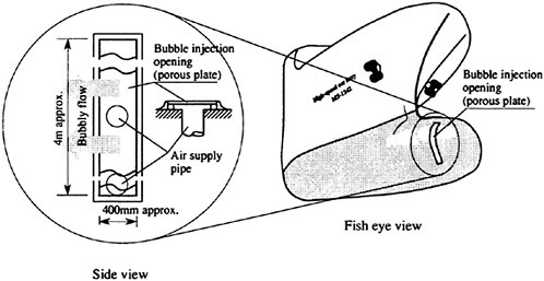
Fig. 16 Car-ferry for estimation example
the pressure estimated by CFD calculation that would be exerted against the bubble injection opening mounted on bulb side as shown in Fig. 16.
We will proceed to estimate in terms of effective horsepower the gain of propulsive power obtained by skin-friction reduction, with the effect of wave-making resistance ignored on the strength of what was discussed above.
We will hence regard the mean resistance reduction ratio CF/CF0 (wetted-surface-averaged skin-friction ratio) to be related solely to skin friction, and that it further does not affect the coefficient for form factor (viscous pressure resistance change).
Hence, the overall resistance reduction ratio
(95)
where
(96)
(97)
The power consumed by compressor is estimated assuming adiabatic compression and no pressure loss on the piping and bubble injection system. The same 288 Κ is assumed for the temperature of seawater and of compressor suction air.
The calculated results are presented in Table 2.
Table 2 Calculated result of power gain
|
QG |
CF/CF0 |
DR |
Comp. power |
Gain |
|
m3/min |
|
% |
kW |
% |
|
100 |
0.9777 |
0.83 |
100 |
0.6 |
|
200 |
0.9557 |
1.64 |
200 |
1.1 |
|
300 |
0.9342 |
2.44 |
300 |
1.6 |
|
400 |
0.9131 |
3.22 |
400 |
2.1 |
|
500 |
0.8925 |
3.99 |
500 |
2.6 |
CONCLUDING SUMMARY
The present study has treated a mathematical model on the flow of a micro-bubble sheet injected from wall.
The model proposed here has extended the conventional model by analyzing the movement of bubble within the flow, to consider the difference in velocity between liquid and gas phase and the shear stress generated by this velocity difference, to constitute a model incorporating mixing length.
The present model has enhanced the agreement obtained with experimental data, by better representing the scale effect, to mark a step forward in the estimation of performance on full-scale ship.
In considering the present model, bubble flow has been classified into three categories by frequency of bubble movement within the turbulent flow. Upon thus defining different categories of flow, cases of frictional resistance reduction could be conceived where turbulence would be suppressed instead of being promoted by bubble presence.
To conclude, frictional resistance reduction by micro-bubble sheet can be considered to promise significant gain in propulsive power, pending solution of a number of questions remaining to be solved.
BIBLIOGRAPHIC REFERENCES
1. McCormick, M.E. and Bhattacharyya, R., “Drag reduction of a submersible hull by electrolysis,” Naval Engineers Journal, Vol. 85, 1973, pp. 11–16
2. Bogdevich, V.G., Evseev, A.R., Malyuga, A.G. and Migirenko, G.S., “Gas-saturation effect on near-wall turbulence characteristics,” Second International Conference on Drag Reduction, Cambridge, England, BHRA Fluid Engineering, paper D2, 1977, pp. 25–37
3. Madavan, N.K., Deutsch, S. and Merkle, C.L., “Measurements of local skin friction in a micro bubble-modified turbulent boundary layer,” Journal of Fluid Mechanics, Vol. 156, 1985, pp. 237–256
4. Madavan, N.K., Deutsch, S. and Merkle, C.L., “Numerical investigation into the mechanisms of microbubble drag reduction,” Journal of Fluids Engineering, Vol. 107, 1985, pp. 370–377
5. Marié, J.L., “A simple analytical formulation for microbubble drag reduction,” Physico-Chemical Hydrodynamics, Vol. 8, 1987, pp. 213–220
6. Kato, H., Miyanaga, M. and Guin, M.M., “Frictional drag reduction by injecting bubbly water into turbulent boundary layer,” Cavitation and Gas-Liquid Flow in Fluid Machinery and Devices, FED-vol. 190, ASME, 1994, pp. 185–194
7. Kato, H., Miyanaga, M., Yamaguchi, H. and Guin, M.M., “Frictional drag reduction by injecting bubbly water into turbulent boundary layer and the effect of plate orientation,” In: Serizawa, A., Fukano, T. and Bataille, J. (eds.) Advances in Multiphase Flow, Kyoto, Japan, Elsevier, Amsterdam, 1995, pp. 85–96
8. Guin M.M., Kato H., Yamaguchi H., Maeda, M. and Miyanaga, M., “Reduction of skin friction by microbubbles and its relation with near-wall bubble concentration in a channel,” Journal of Marine Science and Technology, 1996, Vol. 1, pp. 241–254
9. Watanabe, O., Masuko, A. and Shirose, Y., “Measurements of drag reduction by microbubbles using very long ship models,” Journal of Society of Naval Architects of Japan, Vol. 183, 1998, pp. 53–63
10. Prandtl, L., “Neuere Ergebniss der Turbulenz-Forschung,” Z. Verg. Dtch. Ing., Vol. 77, 1933, pp. 105–114
11. Guin, M.M., “Studies on frictional drag reduction by microbubbles in turbulent boundary layer,” Doctoral thesis, University of Tokyo, 1997
12. Kato, H., Iwashina, T., Miyanaga, M. and Yamaguchi, H., “Effect of microbubbles on the structure of turbulence in a turbulent boundary layer,” Journal of Fluids Engineering, 1998, to be published
13. Tsuji, Y., Morikawa, Y. and Shiomi, H., “LDV-measurements of air-solid two-phase flow in vertical pipe,” Journal of Fluid Mechanics, Vol. 139, 1984, pp. 417–437
14. Gore, R. and Crowe, C.T., “Effect of particle size on modulating turbulent intensity,” International Journal of Multiphase Flow, Vol. 15, 1989, pp. 279–285
15. Clift, R., Grace, J.R. and Weber, M.E., “Bubbles, Drops and Particles,” 1978, Academic Press
16. Saffman, P.G., “The lift on a small sphere in a slow shear flow,” Journal of Fluid Mechanics, Vol. 22, 1965, pp. 385–400
17. Ervin, E.A. and Tryggvason, G., “The rise of bubbles in a vertical shear flow,” Journal of Fluids Engineering, Vol. 119, 1997, pp. 443–449
18. Tomiyama, A., Kataoka, I., Fukuda, T. and Sakoguchi, T., “Drag coefficients of bubbles (2nd report, drag coefficient for a swarm of bubbles and its applicability to transient flow),” Trans. Japan Society of Mech. Eng. (B), Vol. 61, No. 588, 1995, pp. 2810–2817
19. Yoshida, Y., Takahashi, Y., Kato, H., Masuko, A. and Watanabe O., “Simple Lagrangian formulation of bubbly flow in a turbulent boundary layer,” Journal of Marine Science and Technology, Vol. 2, 1998, pp. 1–11
20. Masuko, A., Shirose, Y. and Ishida, S., “Numerical simulation of the viscous flow around ships including bilge vortices”, 17th Symposium on Naval Hydrodynamics, Hague, 1988, pp. 299–314
21. Laufer, J., “Investigation of turbulent flow in a two-dimensional channel,” NACA, Rep. 1053, 1951
22. Doi, Y., Mori, K., and Hotta, T., “Frictional drag reduction by microbubbles,” Journal of Society of Naval Architects of Japan, Vol. 170, 1991, pp. 55–63
DISCUSSION
E.Nikolaev
Krylov Shipbuilding Research Institute, Russia
I congratulate the authors for a perfect paper of fundamental notice which seems to open the way to a new technology in the field of ship resistance reduction. Different technology aimed to the same goal was worked out by Krylov Shipbuilding Research Institute (KSRI) some years ago and was applied to full-scale ships. The KSRI technology was based on the air film method. My questions are as follows: (1) Have the authors compared the two technologies mentioned from the viewpoint of efficiency, and (2) taking into account ship behavior in waves, will it make quite a problem to protect and keep micro-bubble sheet on the hull surface while a ship is rolling, pitching, and swaying?
AUTHORS’ REPLY
Reply to (1): Complete air film separates hull surface from water, which enables to reduce frictional resistance better than micro-bubbles.
Bassin et al.1 has proved that air film technology can be applied to the barge (Speed: 4.1 m/s) with power gain of 20% by means of the full-scale test. On the other hand, micro-bubbles give the car-ferry (Speed: 15.4 m/s) power gain by 2.6% as described in the paper. In the case of a ship that has a lot of flat bottom part and relatively low speed like a barge, air injected from a slit type opening located on the bottom keeps air to be film. In the case of relatively higher speed ship than barge, high speed water flow near the opening disperses the air to be bubbly flow. Flow patterns of air film and bubbly flow depend on ship speed and void fraction. And air film keeping might be difficult subject at high speed.
Reply to (2): Ship motion makes changes of limited stream lines, which makes changes of bubble trajectories. Even if bubble trajectories under the bottom, rolling and pitching makes change of the trajectories. Bubbles rising to free surface faster than without ship motion lowers resistance reduction effect. Research on how to protect from the lowering of the effect should be a future work.
|
1 |
Bassin, A. et al.: Reduction of water-resistance to ship motion due to air supercharge under the bottom, Sudostroyeniye, No. 1, 1968. |
DISCUSSION
Τ.Suzuki
Osaka University, Japan
Thank you for your interesting paper. I have an interest in the method on scale effects you proposed. We, one of the research groups in Japan, have a plan to do full-scale ship tests like your model experiments. In that case, we would like to do physical measurements as well as the measurements of ship speed, propeller revolutions, torque, and/or thrust to check your theory if possible. The most important terms in your theory are void fraction near the wall, αω, and air bubble diameter, I think.
The first question is, do you have any plan to do full-scale ship experiments in the near future?
The second question is, given that the measurements of void fraction and diameter of air bubble at full scale test are quite difficult, then are measurements of wall shear force and velocity gradients near the wall enough to check your theory or not? Thank you.
AUTHORS’ REPLY
Reply to (1): I think myself that we have done as much as we can so long as model scale test is concerned within the present state of the art of measurement technology. I am now looking for a ship for full scale ship test next year.
Reply to (2): A core equation in the theory is Eq. (63). In regard to experimental validation on the asymptotic approximation of Eq. (63) that calculates the friction Cf/Cf0.
An important term is 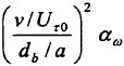 in Eq. (61). Thus, in addition to shear force, near-wall void fraction αω and bubble diameter db should be measured.
If measurement of bubble diameter db is impossible, normal void fraction distribution to the hull surface should be needed because the representative bubble diameter can be calculated by the solution Eq. (80) on the master equation of void fraction.
Spray Formation at the Free Surface of Liquid Wall Jets
T.Sarpkaya, C.Merrill (Naval Postgraduate School, USA)
ABSTRACT
This is an experimental investigation of the ligament and drop formation at the free surface of liquid wall jets, flowing over smooth and sand-roughened plates. Measurements were made with several high-speed imagers, a pulsating laser, and a Digital Particle Image Velocimeter (DPIV) system and analyzed through the use of appropriate software. The wall-jet Reynolds number ranged from 2.4×10⁴ to 4×10⁴, the Froude number from 15 to 30, and the Weber number from 1,500 to 3,000. The positions of the transition and primary breakup as well as the characteristics of the ligament forest and droplets were determined from the digitized images and interpreted in terms of the characteristics of the turbulent boundary layer and a phenomenological model based on our observations and measurements. The emphasis has been on the physics of the phenomenon rather than on the development of empirical relationships.
NOMENCLATURE
|
D |
=diameter |
|
Ddr |
=droplet diameter |
|
Dli |
=mean ligament diameter |
|
Dp |
=ejected plug diameter |
|
Fr |
=Froude number |
|
g |
=gravitational acceleration |
|
ho |
=jet thickness at the edge of the plate |
|
h(x) |
=local jet thickness at x |
|
k |
=mean roughness height |
|
kw |
=wave-number |
|
Lli |
=ligament length |
|
Reh |
=Reynolds number=Uoho/ν |
|
Rex |
=Uox/ν |
|
t |
=time |
|
U |
=streamwise velocity |
|
Uo |
=mean jet velocity at exit |
|
<v'> |
=rms value of v' normalized by Uo |
|
<u'v'> |
=turbulent shear=−u'v'/U2 |
|
Vdr |
=vertical droplet velocity at inception |
|
We |
=Weber number=ρUo2ho/σ |
|
x |
=streamwise distance |
|
xdr |
=distance to droplet inception |
|
xli |
=distance to ligament inception |
|
xtr |
=distance to transition |
|
y |
=vertical axis |
|
z |
=transverse axis |
|
m |
=dynamic viscosity |
|
ν |
=kinematic viscosity |
|
ρ |
=density of water |
INTRODUCTION AND BRIEF REVIEW
The problem of drop formation has developed in many directions and presents different points of view and different goals for various disciplines. The fact that it continues to attract the attention and energy of impressively large numbers of researchers attests to its technological importance and, just as importantly, to its intellectual challenge.
The drop formation in a circular liquid jet has attracted the most mathematical and experimental interest for obvious reasons. The sprays generated from spray roots and their rupture into smaller particles have been of major practical interest in the field of combustion. There are many other applications where a continuum becomes a two- or multi-phase flow through drop dynamics (agriculture, naval architecture, irrigation, decorative fountains, ship-plunging, ink-jet printing, perfumery, deuterium microspheres and laser fusion, chemical warfare, just to name a few). The impetus for the present research comes from the need to understand the physics of spray formation at the free surface of turbulent wall jets and, subsequently, the breakup of bow sheets into fine spray. The latter may help to reduce the visual and
radar signatures of ships subjected to the accumulation of water mass on exterior surfaces (topside ice, equipment and sensor degradation, reduced vision, enhanced wake and ship signature, bow glow with bioluminescent organisms, etc.).
A critical review of the extensive literature has shown that the breakup of jets and sheets depends strongly not only on the conditions governing their creation but also on the conditions surrounding their subsequent evolution under the influence of several competing internal/external influences such as turbulence, gravity, surface tension, liquid-sheet geometry, surface shear, roughness of the contact surface(s), velocity distribution in the sheet, temperature distribution in the jet, pressure fluctuations within and outside the liquid sheet, acoustic excitation, external flows (e.g., wind), intentionally imposed disturbances, and foreign particles (e.g., air, dust). It is generally agreed that eddies accelerated by the internal motion of the fluid tear into irregular shapes and give rise to ligaments (threads) and droplets. The ligaments may initially appear as large undefined volumes of water or nearly transparent sheets. These shapes then continue to rupture into smaller particles until the surface tension forces inhibit them from further disintegration under the prevailing environmental conditions.
The investigation described herein deals with the breakup of a more specific flow, namely that of a liquid wall jet with a free surface (free wall jet). It must be emphasized that the only apparent difference between the much-studied “wall jet” and the one described herein is that whereas the “wall jet” discharges into a medium of identical fluid, the liquid or free wall jet is bounded by a smooth or rough wall below and a free surface above (air/water interface). The resulting flow is intended to simulate the inception of bow sheet/spray flows for an observer on board the ship. In the present experiments, the jet issues (a) from a nozzle and (b) from a streamlined gate at the upstream end of a recirculating free-surface water tunnel. In both cases the jet is maintained in a steady state as long as desired for a detailed measurement of the characteristics of ligaments, droplets, and bubbles. No attempt has been made to develop empirical relations between particular characteristics of the flow and the Weber number, Reynolds number, Froude number, and the relative roughness.
The investigation of a free wall jet, though quite specific, still raises a large number of fundamental questions some of which are undoubtedly common to all spray phenomena: How important is the nozzle shape (two dimensional or axisymmetric) on the subsequent evolution of the jet? If turbulence is ultimately responsible for the ejection of the lumps of fluid from the jet body, then what is responsible for the turbulence in a wall-jet with free surface: External aerodynamic excitation, internal instability and the wall of the partially wall-bounded flow, or both? How is the free-surface/turbulence interaction modified by ejections? How does that modification manifest itself along the jet? How does the shape of the free surface (curvature, shear) affect the mass, momentum, and vorticity flux across the free surface? Considering the fact that in internal turbulent flows more momentum is transferred from the flow to the walls, how does the free surface affect the partitioning of the jet-momentum flux between the bottom wall, the free surface, and the jet? What role does the condition of the wall surface play in the ejection-sweep cycle or in the relative magnitudes of the components of the stress tensor? Does roughness enhance the mass, momentum, and vorticity flux towards and out of the free surface? Clearly, this is a very complex two-phase flow problem, requiring the understanding of the internal as well as the surface flow, even for a wall-bounded and relatively well-defined jet geometry.
Partial answers to some of the foregoing questions have been provided by several investigators (1–5) prior to 1977, and more recently by Wu et al. (6) and Dai et al. (7) towards the quantification of the characteristics of spray phenomena on annular liquid wall jets about axisymmetric rods. These have shown that the qualitative features of flows over spillways, plunge pools, open water waves, and axisymmetric rods are quite similar. Their observations and measurements have also suggested that turbulence generated on the wall propagates across the flow and reaches the interface and roughens the free surface. This laminar-turbulent transition at the air/water interface is followed by a region of turbulent breakup where a forest of ligaments rise above the free surface. Some, but not all, of these ligaments give rise to one or more droplets. Subsequently, the free-surface activity gradually subsides due to loss of momentum. The positions of the transition and primary breakup as well as the character of the ligament forest can be affected by trip wires, local or uniformly-distributed roughness, and possibly by aerodynamic effects.
The question of the origin of turbulence and the aerodynamic effects were addressed by a number of investigators (4–8). It has been concluded that the origin of turbulence is the same as in all internal flows (instability of the flow and the walls) and not the relative motion at the liquid/air interface. In other words, the aerodynamic effects do not play measurable roles in turbulence generation and do not appear to interact with the spray generation. However, the question of how turbulence selectively accelerates and ejects parcels of fluid across the liquid/air interface remains unclear. Equally unclear is the profound effect of roughness in ligament generation and of the air bubbles created within the jet by the entrainment of air carried by the ligaments and droplets falling back on
the free surface. One rather obvious reason for this is the lack of detailed velocity and turbulence measurements in free wall jets. In spite of its major importance, there has never been an experiment with a liquid wall jet, with ligaments and spray, where the distributions of the mean as well as the instantaneous flow fields and the complete Reynolds stress tensor were measured at numerous sections downstream from the nozzle. What is measured (8) is for very low-Froude-number flows where the free surface exhibits nothing more than small irregular fluctuations. There are, to be sure, numerous hot-wire and LDV measurements in wall jets (air into air or water into water) and in closed conduits (pipes and rectangular channels). Some of these measurements are accompanied by numerical simulations (DNS, LES, RANS) at relatively low Reynolds numbers.
APPARATUS AND PROCEDURES
A two-dimensional nozzle of aspect ratio of 32 (Fig. 1a) was attached to a large U-shaped water tunnel (10 m wide and 7.5 m high) at a suitable location along one of its two vertical towers (9, 10). The upstream face of the nozzle (facing the tunnel wall) was carefully streamlined so as to provide a smooth entrance into the nozzle (Fig. 1b). It was known (11) early on that the nozzle design has a significant impact on the characteristics of the resulting jet and that data from various sources cannot be compared on the basis of Reynolds and Weber numbers alone. The nozzle shown in Figs, 1a and 1b embodies all of the past recommendations (3–5, 11–12) (e.g., a gradual geometric transition, continued acceleration, earlier transition on the walls and a thinner turbulent boundary layer).
The jet exited from the nozzle upon the removal of a cylindrical gate and flowed, after a short free flight (about 80 mm), over the horizontal test plate. The jet surface had a fine-grained texture on emergence due to the turbulent surface layer. Only for relatively low velocities did the jet have an extremely smooth clear surface, as if it were frozen. In either case, however, the jet was essentially non-turbulent by the time it reached the edge of the plate.
The discharge was collected in a trough and then pumped back into the opposite tower of the U-shaped tunnel. A foam divider, sandwiched between two heavy wire screens, was inserted near the mid-length of the horizontal section of the tunnel. These precautions have indeed assured that the flow entering into the nozzle was free from disturbances, as verified by flow visualization with dye (food coloring). With this arrangement it was easy to maintain constant jet velocities from 3 m/s to 6.5 m/s indefinitely. Suffice it to note that the use of a nearly ideal nozzle, long observation and measurement times, and reliance on high-speed video (HSV), DPIV, and Laser-Induced Florescence (LIF) made the entire apparatus particularly unique for the investigation under consideration. The additional advantages of the system were the relative ease with which the test plates (smooth or rough) can be interchanged, bodies of special interest can be mounted, and the flow can be illuminated and photographed.
The basic test plate was a 33 cm wide and 120 to 180 cm long smooth Plexiglas sheet, mounted horizontally and rigidly on adjustable supports. The upstream edge of each plate was beveled with a sharp edge at an angle of 30 deg. from the horizontal. The elevation of the sharp-edge of the horizontal plate was positioned carefully so as to capture only the top 6 mm of the 8.5 mm jet. Some plates were sand-roughened carefully to achieve the desired relative mean roughness height of k/ho (from 0.02 to 0.13). Some plates had as many as five strategically-located dye holes along a line about 60 mm from the edge of the plate for flow visualization. The use of tripping wires or tripping sand-strips were considered and even subjected to trial runs. However, the realization that the resulting turbulent motion at any section of a smooth flat plate may neither be representative of the bow/sheet interaction nor accurately depict the ejection-sweep processes in liquid wall jets with a free surface, led to the use of only smooth or only uniformly-roughened surfaces with no tripping wires. It is a well-known fact that the near-wall region is characterized by a randomly recurring burst cycle (the violent ejection of the low-speed fluid towards the free surface and the down sweep of higher-speed fluid towards the wall). Roughness renders the mean flow three dimensional in the roughness sublayer, gives rise to higher energy ejections not existing in smooth wall flows, rapidly increases the thickness of the jet by extracting larger momentum, and thus changes not only the character of the ejections and sweeps but also the interaction of the coherent structures with the free surface. Since the free-surface structures (including ligaments and droplets) are an outgrown manifestation of the bursting process in the wall region, the behavior of the turbulent motion generated by a uniformly-roughened surface cannot be duplicated by that of a trip-wire-generated turbulent motion over a smooth wall. There are, to be sure, circumstances where trip wires serve the intended purposes well (e.g., precipitate transition, delay separation).
The second test facility consisted of a high-speed free-surface water tunnel (about 8 m3) and used primarily for the acquisition of velocity and turbulence data through the use of a DPIV system, in addition to HSV recordings of the bubbles, ligaments, and droplets. The open test section was 50 cm wide, 50 cm deep, and about 6 m long and had large Plexiglas windows on all three faces. During the off-test periods, a small pump continuously filtered the tunnel
water through a micro filtration system to remove rust and other suspended fine particles, down to about 10 μm, from the water. The wall jet was created by placing an adjustable streamlined gate at the upstream end of the tunnel where the closed section joined the free-surface section. Smooth and sand-roughened Plexiglas plates were placed at the bottom of the test section. The jet velocities of about 6 m/s were easily achieved through the use of a 50 Hp pump.
Instrumentation for both facilities consisted of several high-speed cameras with frame rates from 250 frm/s to 10,000 frm/s (with shutter speeds from 1/250 to 1/5000 sec) and a DPIV system. The recordings of the jet surface, ligaments, droplets, and the scales inscribed on the plate were made along the jet (within a 1.6 m long and 30 mm wide centrally-located strip, along the longitudinal axis of the plate) through the use of proper lenses and back and front lighting. This assured that a single ligament or a droplet could be tracked during its lifetime, from its creation to its return to the body of the jet, without being obscured by the shadows of ligaments in neighboring planes.
The video images were first carefully reviewed to identify a number of representative ligaments (with or without droplets) whose motion could be traced with little or no ambiguity. The diameter, volume, tip velocity, and lifespan of ligaments, the wave-number of the axisymmetric disturbances, time of droplet formation, droplet size and velocity, free surface velocity, the temporal mean of the local jet thickness, in addition to the distances to the region of transition and roughness, to the region of surface distortions and ligaments, and to the region of ligaments and droplets were evaluated through the use of a suitable software (Optimus-MA). It is of some importance to note that the characteristic diameter of a ligament was evaluated by drawing a contour around the ligament and automatically evaluating the enclosed area above the free surface and, therefrom, the characteristic diameter and volume.
The determination of the ligament length and diameter involves some uncertainty because the beginning of the ligament is not precisely definable (due to surface distortions) and the assumption of axisymmetry of the ligament cannot always be ascertained. High-speed video images taken directly from above the jet as well as the visual observations with a high-speed stroboscope have shown that well-defined ligaments were almost always nearly axisymmetric. Nevertheless, the experimental uncertainties cannot be lowered to less than about 20 percent primarily due to scale effects, highly turbulent nature of the flow, uniqueness of each ligament, and the sampling limitations.
The wall-jet Reynolds number ranged from 2.4×10⁴ to 4×10⁴, the Froude number from 15 to 30, and the Weber number from 1,500 to 3,000. Only clean water was used in the experiments. No attempt was made to change either the viscosity or the surface tension through the use of other fluids and/or surfactants.
RESULTS AND DISCUSSION
The evolution of the free surface has been described in many interesting ways by a large number of previous workers (1–7). Here, we will describe it in terms of four stages (the first three are shown in Figs. 2a–d): (i) The region of transition and roughness in which the turbulent boundary layer reaches the free surface and measurably roughens it but there are not yet any ligaments (Fig. 2a, an LIF image); (ii) The region of surface distortions and ligaments in which there are large surface distortions and ligaments but no drop formation (Figs. 2b and 2c, LIF and HSV images); (iii) The region of ligament forest and droplets in which there are ligaments giving birth to one or more drops as well as ligaments with no drops, (Fig. 2d, HSV images); and, finally, (iv) The region of decreasing activity in which surface manifestations gradually subside in a jet which has lost a great deal of its momentum to both the wall and the free surface during its first three stages.
The region of transition and turbulence has been measured in all cases with as much accuracy as possible considering the fact that it is a gradual process (for smooth plates) and subject to some uncertainty. Only the smooth plate case can be predicted with some degree of confidence through the use of an approximate analysis, assuming the transition of the free wall jet to be similar to that of an unbounded laminar boundary layer (13). The transition on sand-roughened plates is a more complex problem (14). It can be calculated numerically and only approximately through the use of suitable velocity profiles appropriate to rough-wall boundary layers (15–16). The observations have shown that turbulence begins almost immediately after the start of the plate and reaches the free surface within 25ho to 40ho, depending on k/ho (from 0.02 to 0.13), as shown in Fig. 3. Also shown in Fig. 3 are the distances to the inception of ligament and droplet formation. Clearly, the rougher the surface, the shorter is the distance to transition and to the ligament and droplet formation. It appears that the said distances cease to depend on roughness beyond some minimum value of k/ho (about 0.06). The actual thickness of the jet [h(x)] increases (see Fig. 4) with x/ho and is dependent, to varying degrees, on the fundamental parameters governing the phenomenon (Reh, Rex, Fr, We, and k/ho), provided that the aerodynamic effects are negligible. Thus, the distances to important events need to be related to the local mean jet height h(x) since it defines not only the vertical extent of the region in which ejections, sweeps, and eddy motions
take place but also the characteristics of the free surface and of the ligaments and droplets. Figure 4 shows that the jet thickness nearly doubles even for a smooth plate. The effect of roughness on h is even more dramatic.
The attention will now be focused on the creation and subsequent motion of a single droplet in the region of ligament forest and droplets. The six frames in Fig. 2d (time and jet: left to right) show, in suitable time intervals, the evolution of a representative droplet and the changes in the structure of the mother ligament (Rex=2.3×10⁶, Reh=3.55×10⁴, Fr=25.8, We=3010, k/ho=0.06). It is seen that the ligament under observation is leaning slightly forward (some lean forward and some lean backward), has several waves along its length and a diameter smaller than that of the droplet. It is also seen that the length of the disturbance wave increases, as the ligament diameter decreases towards the tip, giving the ligament the shape of a truncated cone. Figure 2d also shows that neither the inclination of the ligament nor its position relative to the free-surface topography changes with time. In fact, Figure 2d as well as hundreds of others like it have shown unambiguously that the external aerodynamics has no measurable effect on the spray formation, conforming a fact previously noted by others (see, e.g., 4–7).
The characteristics of ligaments and droplets will now be discussed through the use of a number of plots. Figure 5a shows the distribution of the ratio of the ligament length to ligament diameter, Lli/Dli (the slenderness ratio), just prior to pinch-off and droplet formation, for a large number of realizations for a relative roughness of k/ho=0.13 and a Weber number of We=2,900. The mean value of the ligament slenderness ratio depends on the (k/ho, We) combination as shown in Fig. 5b. Clearly, for a given We, the ligaments become more slender with increasing relative roughness. Also, for a given roughness ratio (say 0.13), Lli/Dli increases with increasing Weber number. The overall average of Lli/Dli is about 5 with a standard deviation of 1.9, as seen in Fig. 5b. Clearly, there is, as expected, significant variations from one ligament to another. Nevertheless, the values noted above provide a good starting base towards the understanding of the physics of ligaments.
Figures 5c and 5d show the relative ligament length Lli/ho and its relatively strong dependence on roughness. The overall average of the normalized ligament length (prior to drop formation) is about 2. Figure 6a shows the persistence of normalized ligament volume, ![]() again just prior to drop formation, for various pairs of k/ho and We. Figure 6b gives a summary of the mean values of
again just prior to drop formation, for various pairs of k/ho and We. Figure 6b gives a summary of the mean values of ![]() in terms of (k/ho, We) combinations. Apparently, the ligament volume increases considerably with roughness for a given We. The same is also true for a doubling of the Weber number for k/ho=0.13 (first and fourth columns). The overall average of the ligament volume (shown in the last column) is about 0.25.
in terms of (k/ho, We) combinations. Apparently, the ligament volume increases considerably with roughness for a given We. The same is also true for a doubling of the Weber number for k/ho=0.13 (first and fourth columns). The overall average of the ligament volume (shown in the last column) is about 0.25.
Figure 7 shows the ratio of the drop-diameter to ligament-diameter, Ddr/Dli, for the entire data. It has a mean value of 1.6. Thus, on the average, a small piece of the ligament (about 2.72 Dli long) is pinched off from the end to form a droplet. Figures 8 shows the histogram or the persistence of the drop diameter, normalized by ho, for all values of k/ho and We. It has a mean value of 0.61. Figure 9 shows the same data for each combination of k/ho and We. Apparently, Ddr/ho does not appreciably depend on the roughness and Weber number within the range of the present measurements. Figure 10 shows the diameter of the ligament, normalized by ho. It has a mean value of about 0.4.
Figure 11a shows the angle the ligament makes with the horizontal plane. An angle less than 90° means the ligament is leaning backwards as it travels forward. On the average, the ligaments lean slightly backward (about 14° from the vertical). Figure 11b shows the entire data in terms of the relative roughness and the Weber number. The variation of α within the range shown is negligibly small.
The visible disturbance wave-number kw, just prior to drop formation, is shown in Fig. 12 in terms of the mean diameter of the ligament. The overall average is 1.75 with a standard deviation of 0.4. Rayleigh (17) has shown that the maximum growth rate of an axisymmetrical disturbance occurs at a wave-number of kw=0.697. The difference between that found in the present investigation for the breakup of a ligament and that of Rayleigh for the development of disturbances on a capillary jet is attributable in part to the fact that near the tip the maximum diameter of the wave is about 75% smaller than the mean diameter of the ligament, the length of the wave is about 80% larger than the mean, and the shape of the amplified wave is more like an elongated ellipsoid. In fact, it can be verified that the use of the values prevailing near the tip leads to a wave-number of about 0.75 which is closer to that expected for the capillary jets. However, it is not our intention to assert here that the wave-number for a ligament should be identical to that predicted by Rayleigh (17) for a number of reasons: the wall jet is not an axisymmetric laminar jet and the waves seen on the ligaments are fully developed disturbances, not infinitesimal instabilities. Figure 13 shows the mean values (and one standard deviation) of the drop Reynolds number based on the vertical
velocity of the drops at the time of their birth for each combination of k/ho and Weber number. The average Reynolds numbers is about 800.
We now make an attempt to relate the ligaments and droplets to the internal structure of the flow. Postulating a vertical fluid column (say a plug) of diameter Dp and height h(x) in the jet, as seen in Fig. 14, and equating its volume to that of an average ligament (about ![]() as seen Figs. 6a and 6b), one finds that h(x)/Dp=π1/2[h(x)/ho].3/2 Noting that h(x)/ho in Fig. 4 varies from about 2 to 2.5 (for the rough wall) as x/ho varies from about 50 to 125 (the range in which most of the ligament/droplet data were taken), one finds that h(x)/Dp varies from 5 to 7. As stated in connection with Fig. 5a, the mean values of the ratio of the ligament length to ligament diameter (Lli/Dli) vary from about 4.5 to 6, with an overall average of about 5.2. In other words, a ligament and a plug have, for all intents and purposes, nearly identical characteristics. Thus, one may postulate that such a plug is launched upwards by an ejection and becomes a ligament. The initial plug velocity Vp needed to increase its potential energy by
as seen Figs. 6a and 6b), one finds that h(x)/Dp=π1/2[h(x)/ho].3/2 Noting that h(x)/ho in Fig. 4 varies from about 2 to 2.5 (for the rough wall) as x/ho varies from about 50 to 125 (the range in which most of the ligament/droplet data were taken), one finds that h(x)/Dp varies from 5 to 7. As stated in connection with Fig. 5a, the mean values of the ratio of the ligament length to ligament diameter (Lli/Dli) vary from about 4.5 to 6, with an overall average of about 5.2. In other words, a ligament and a plug have, for all intents and purposes, nearly identical characteristics. Thus, one may postulate that such a plug is launched upwards by an ejection and becomes a ligament. The initial plug velocity Vp needed to increase its potential energy by ![]() and the surface energy by may be reduced to
and the surface energy by may be reduced to
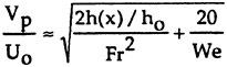
For the majority of the experiments, (We=2,900, Fr=26, and 2<h(x)/ho<2.5), one has Vp/Uo≈0.1. The contribution of the term involving Fr2 becomes increasingly small as the jet velocity increases. Then the ejection phenomenon is governed primarily by the inertial and surface tension forces. For a jet with an initial velocity of Uo=6 m/s, Vp varies from about 0.46 m/s to 0.52 m/s with Δt=h(x)/Vp=25 ms and Δx/h(x)=11. We have carried out extensive DPIV measurements, using the same wall jets, in order to explore the plausibility of the proposed model. It was thought that the characteristics of the flow in a highly disturbed wall jet, with ligaments, droplets, and occasional air bubbles (resulting from the entrainment of air due to the impact and penetration of droplets on the free surface when the Weber number exceeds a critical value), cannot be deduced from the existing pipe-flow or boundary layer measurements (see, e.g., 14–16, 18–20). Representative data are shown in Fig. 15 where the rms values of <u'> and <v'>, normalized by Uo, are shown as a function of y/d. As suspected, the rms values shown in Fig. 15 are significantly different from those obtained in pipes and boundary layers over rough walls (14–16,18–20). Furthermore, <v'> is quite close to Vp/Uo, to provide the necessary kinetic energy to launch the fluid plug to the desired height, including the gravitational and surface tension effects.
It is not the purpose of the foregoing to reduce a complex turbulent motion to a ligament launching mechanism, but rather to point out that it is possible to eject columns of fluid out of the body of the jet and form ligaments of the order of local jet thickness, provided that there is sufficient kinetic energy to sustain the ejection over a vertical displacement of h(x) before the plug looses its coherence. It is a well-known fact that there are quasi-periodic coherent structures which occupy the whole boundary-layer depth and live long enough for coherence to be preserved over streamwise distances of 10d to 20d. In our experiments this would equal to 10h(x) to 20h(x). In other words, the predicted value of Δx/h(x)=11 is well within the realm of possibility.
Raupach (19) has shown in connection with his work on turbulent boundary layers over smooth and rough walls that the streamwise separation between consecutive large structures is 3.6d for smooth walls and 2.1d for rough walls. He has further shown that as the roughness increases (i.e., the wall becomes a stronger momentum sink), a larger number of large structures develop per unit streamwise length of the boundary layer, i.e., the frequency of the structures increases with roughness. Our observations with three sizes of roughness are in conformity with Raupach’s (19) findings.
CONCLUSIONS
An experimental investigation of the ligament and droplet formation at the free surface of liquid wall jets, flowing over smooth and sand-roughened horizontal plates, has been carried out. The data deduced from the HSV images and DPIV measurements have shown that the laminar-turbulent transition at the air/water interface is followed by a region of turbulent breakup where a forest of ligaments rise above the free surface. Some, but not all, of these ligaments give rise to one or more droplets. Subsequently, the free-surface activity gradually subsides due to loss of momentum. The positions of the transition and primary breakup as well as the character of the ligaments (length, diameter, instability waves, inclination) and droplets (diameter, velocity) have been determined through the use of a large number of measurements for both smooth and sand-roughened walls.
The DPIV measurements (unique for liquid wall jets) have shown that the rms values of the velocity fluctuations are significantly different from those encountered in turbulent pipe flows and boundary layers, as one would have expected on the
basis of large-scale surface deformations and their effect on a flow of relatively small vertical extent The form drag of roughness serves as an effective arrest mechanism and increases <v'>, renders the flow three-dimensional near the wall, and forms a passive reservoir of low momentum fluid which is drawn on during ejection phases, as in the case of the boundary layer flow over rough walls (19). This leads to extremely violent ejections, with ejected fluid rising almost vertically from between the interstices of the roughness elements. It is seen that the ejections which are strong enough to reach the free surface, after some time, give rise to ligaments and droplets whose number and intensity increase with increasing roughness. In other words, there appears to be a universal ejection-type momentum transport mechanism, possibly extending across the entire thickness of the jet, as in the case of normal boundary layer flows (19).
The similarity of the geometrical characteristics of an average ligament to those of an idealized vertical fluid plug (the mean values of the ratio of the ligament length to ligament diameter vary from 4.5 to 6, with an overall average of about 5.2) and of the vertical velocity needed to eject it to the desired height above the free surface (Vplug/Ujet≈ 0.1) to <v'> of the ejections (from about 0.06 to 0.10 as seen in Fig. 15) are supported by our DPIV data and by the previous works on boundary layers. The smooth walls do not arrest the flow near the wall, do not increase <v'> to sufficiently high values, and do not create a passive reservoir of low momentum fluid which may be drawn on during ejection. Thus, only at much higher Reynolds and Froude numbers that one can expect to generate ligaments and droplets over smooth surfaces. The fact that the surface roughnesses, and the Reynolds and Froude numbers encountered in our experiments are quite similar to those encountered in bow sheet/spray flows suggests that smoother bow surfaces with suitable curvatures may help to alleviate the spray problem.
ACKNOWLEDGMENTS
This investigation has been supported by the Office of Naval Research under contract N0001498WR20009. We are particularly indebted to Dr. Edwin P.Rood for his continuous guidance and encouragement.
REFERENCES
1. Townson, J.M., Free Surface Hydraulics, 1st ed., Unwin Hyman, London, 1988, Chapt. 6.
2. Phinney, R.E., “The breakup of a Turbulent Jet in a Gaseous Atmosphere,” Journal of Fluid Mechanics, Vol. 60, Pt. 4, 1973, pp. 689–701.
3. McCarthy, M.J., and Malloy, N.Α., “Review Of Stability of Liquid Jets and the Influence of Nozzle Design,” Chemical Engineering Journal, Vol. 7, No. 1, 1974, pp. 1–20.
4. Hoyt, J.W., and Taylor, J.J., “Waves on Water Jets,” Journal of Fluid Mechanics, Vol. 88, Pt 1, 1977, pp. 119–123.
5. Hoyt, J.W., and Taylor, J.J., “Turbulence Structure in a Water Jet Discharging in Air,” Physics of Fluids, Vol. 20, Pt 2, No. 10, 1977, pp. S253–S257.
6. Wu, P.-K., and Faeth, G.M., “Onset and End of Drop Formation Along the Surface of Turbulent Liquid Jets in Still Gases,” Physics of Fluids A, Vol. 7, No. 11, 1995, pp. 2915–2917.
7. Dai, Z., Chou, W.-H., and Faeth, G.M., “Drop Formation due to Turbulent Primary Breakup at the Free Surface of Plane Liquid Wall Jets,” Physics of Fluids, Vol. 10, No. 5, 1998, pp. 1147–1157.
8. Finley, P.J., Khoo, C.P., and Chin, J.P., “Velocity measurements in a thin turbulent water layer,” La Houille Blanche, Vol. 21, 1966, pp. 713–721.
9. Sarpkaya, T., “In-Line and Transverse Forces on Cylinders in Oscillatory Flow at High Reynolds Numbers,” Journal of Ship Research Vol. 21, 1977, pp. 200–216.
10. Sarpkaya, T., “Force on a Circular Cylinder in Viscous Oscillatory Flow at Low Keulegan-Carpenter Numbers,” Journal of Fluid Mechanics, Vol. 165, 1986, pp. 61–71.
11. Dombrowski, N., and Fraser, R.P., “A Photographic Investigation Into the Disintegration of Liquid Sheets,” Philosophical Transactions of the Royal Society of London, Vol. 247, No. A924, 1954, pp. 101–130.
12. Rouse, H., and Abol-Fetouh, A.-H., “Characteristics of Irrotational Flow Through Axially Symmetric Orifices,” Journal of Applied Mechanics, Vol. 17, 1950, pp. 421–426.
13. Schlichting, H., Boundary-Layer Theory, McGraw-Hill, 7th ed., 1987, pp. 636–640.
14. Feindt, E.G., “Untersuchungen uber die Abhangigkeit des Umschlages Laminar-Turbulent von der Oberflachenraughigkeit und der Druckverteilung,” Jb. 1956 Schiffbautechn. Ges., Vol. 50, 1957, pp. 180–203.
15. Pimenta, M.M., Moffat, R.J., and Kays, W.M., “Turbulent boundary layer: An experimental study of the transport of momentum and heat with the effect of roughness,” Report HMT-21, 1975, Thermosciences Div., Dept. of Mechanical Engineering, Stanford University.
16. Ligrani, P.M., Moffat, R.J., and Kays, W.M., “The thermal and hydrodynamic behavior of thick, rough-wall, turbulent boundary layers,” Report HMT-29, 1979, Thermosciences Divison, Dept. of Mechanical Engineering, Stanford University.
17. Lord Rayleigh, “On the Instability of Jets,” Proceedings of the London Mathematical Society, Vol. 10, 1879, pp. 4–13, as quoted in Scientific Papers by Lord Rayleigh. NY: Dover Publications, 1945.
18. Klebanoff, P.S., “Characteristics of Turbulence in a Boundary Layer with Zero Pressure Gradient,” NACA Technical Note, 3178, 1954.
19. Raupach, M.R., “Conditional Statistics of Reynolds Stress in Rough-Wall and Smooth-Wall Turbulent Boundary Layers,” Journal of Fluid Mechanics, Vol. 108, 1981, pp. 363–382.
20. Grass, A.J., “Structural Features of Turbulent Flow over Smooth and Rough Boundaries,” Journal of Fluid Mechanics, Vol. 50, 1971, pp. 233–255.
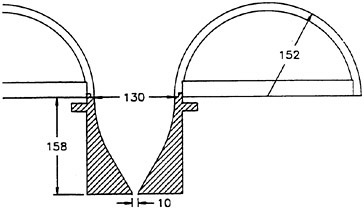
Fig. 1a A partial cross-section of the nozzle.

Fig. 1b A view of the upstream end of the nozzle.
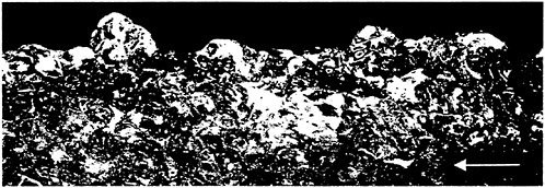
Fig. 2a A pulsed-laser photograph of the transition and roughness region in which the turbulent boundary layer reaches the free surface and measurably roughens it.
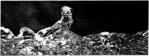
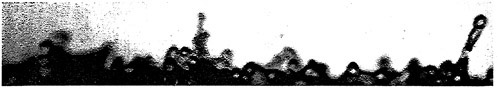
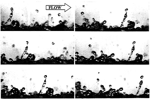
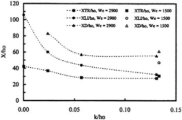
Fig. 3 Distances to the onset of transition and ligament- and droplet formation for various k/ho.
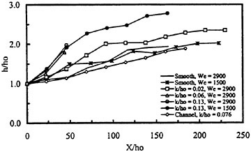
Fig. 4 The variation of the jet thickness along the plate for smooth and representative rough-plate conditions.
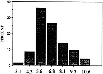
Fig. 5a Histogram of the ratio of the ligament length to ligament diameter, (k/ho=0.13).
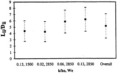
Fig. 5b Mean values of the ligament slenderness ratio for various combinations of (k/ho and We).
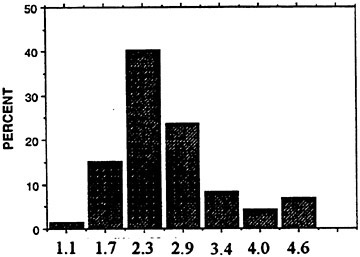
Fig. 5c Histogram of the ligament length normalized by ho, (k/ho=0.13).
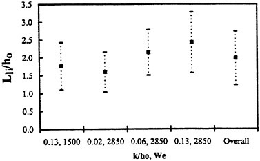
Fig. 5d Mean values of Lli/ho for various combinations of (k/ho and We).
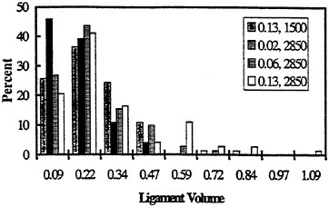
Fig. 6a. Histogram of the normalized ligament volume just prior to drop formation.
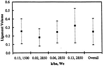
Fig. 6b. Mean values of the normalized ligament volume for various combinations of (k/ho and We).
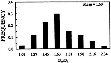
Fig. 7 Histogram of the ratio of the drop diameter to ligament diameter for all runs.
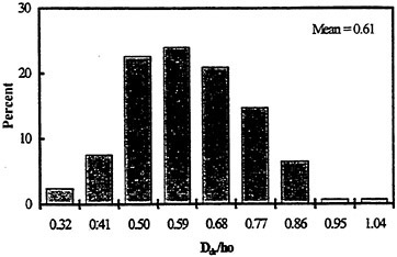
Fig. 8 Histogram of the normalized drop diameter for all flat plate data (mean value=0.61).
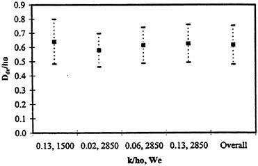
Fig. 9 Mean values of the normalized drop diameter for various combinations of (k/ho and We).
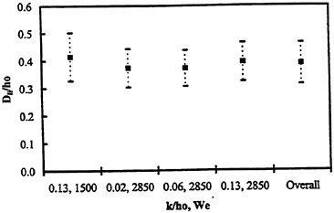
Fig. 10 Mean values of the normalized ligament diameter for various combinations of (k/ho and We).
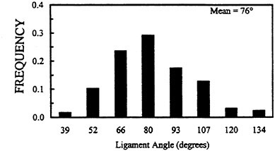
Fig. 11a Histogram of the ligament angle (mean value=76 deg.).
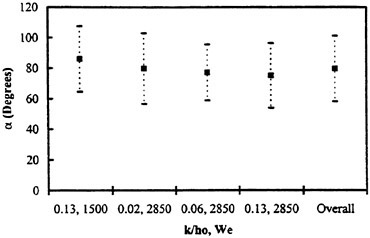
Fig. 11b Mean values of the ligament angle for various combinations of (k/ho and We).
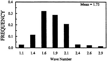
Fig. 12 Histogram of the wave number for all tests (mean value=1.75).
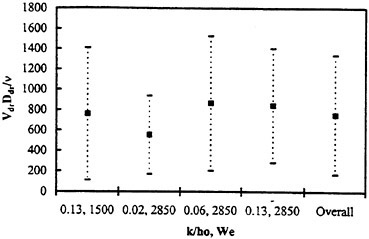
Fig. 13 Mean values of the drop Reynolds number for various combinations of (k/ho and We).

Fig. 14 An actual ligament (left) and its idealized form (right).
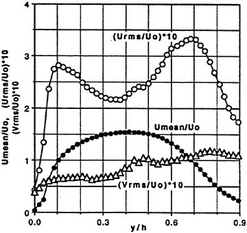
Fig. 15 Normalized velocity and the rms values (×10) of the velocity fluctuations.
DISCUSSION
G.Hearn
University of Newcastle Upon Tyne, United Kingdom
This is the second occasion during the conference in which Prof. Sarpkaya has provided physical insight regarding natural phenomena. Since it is from such physical insight that one ultimately seeks to provide a mathematical model, and hence engineering design capability, may I congratulate and thank you for today’s very clear, precise and fundamental explanation of the liquid wall jet phenomenon.
May I now ask a question related to the spray formation at the bow of the fast moving craft? In your experimental set up, the jet is brought into contact with flat or curved plates. Considering the bow as a complicated wedge, would you expect any of the characteristics of the jet to be radically modified? In other words, will it be necessary to modify your apparatus further?
DISCUSSION
J.W.Hoyt
San Diego State University, USA
I would like to congratulate Prof. Sarpkaya for a marvelous paper with spectacular photographs. My question is: Why do the spray ligaments lean backwards?
AUTHORS’ REPLY
The questions and kind words of Professors Grant E.Hearn and Jack W.Hoyt are very much appreciated.
Regarding the effect of bow geometry, we have carried out a number of additional experiments during the past two years with symmetrical wedges (upright or inclined). The results of these experiments were not reported in the paper partly because of their more case-specific nature and partly because there was much to be learned from experiments idealized enough to reveal physics and broad enough to be relevant. Suffice it to note that even though specific characteristics of the filaments and droplets did not significantly change, the distance at which they have occurred has changed with the angle of wedge and its forward to backward inclination. There is no doubt that the complicated geometry of a bow may affect not only the filament/droplet distribution but also the position along the bow where the wall jet becomes a free jet. The bow-shape effects, the consequences of increasing or decreasing the jet thickness, and the use of sea water in lieu of tap water are now being investigated systematically.
As to the reasons for the ligaments leaning mostly backwards, one may imagine a ligament as a cylindrical eddy of vertical extent h(x) ejecting with a relative average velocity v while its submerged part is subjected to a relative average velocity of u in the streamwise direction. This should lead to mostly backward leaning filaments. If, with some poetic license, one assumes that v is about four times u, then the angle of inclination from the vertical becomes about 14 degrees. This, in fact, is the average of all the filament angles we have measured. Simplistic though the explanation may be, it is hard to find a better one. Again, we thank Professors Grant E.Hearn and Jack W.Hoyt for the opportunity they have accorded to us to expand on two very important questions.
Internal Gravity Waves Excited by a Body Moving in a Stratified Fluid
V.Borovikov,1,2 V.Bulatov,2 M.Gilman,2 Y.Vladimirov2
(1Benemerita Universidad Autonoma de Puebla, Mexico, 2Russian Academy of Sciences, Russia)
The aim of this talk is to describe the user-oriented computer code composed for the numerical calculation of the field of internal gravity waves (abbreviated as IW hereafter) excited in a layer of arbitrary stratified fluid by a movig thin solid body. The linear approximations for the equations of IW and for the boundary conditions at the body’s surface are used. The IW field is expressed in terms of integrals from the Green’s function of IW equation. The code uses the analytic and asymptotic expressions for the Green’s function obtained in (1,2,3) and summed up in (4). To obtain the sought-for values of IW field it is sufficient to introduce the set of points in which we seek for the field; the table of density values as a function of depth, the table describing the body’s shape; and its velocity and depth. The time necessary to calculate by PC the field in fixed point has order of few seconds. Since the calculations are performed with a guaranteed accuracy, these codes can be used not only for comparing theoretical calculations with experiment but for testing more complicated codes using non-linear equations in particular case of linear approximation. The algorithm of IW field evaluation and some examples of the IW numerical calculation are depicted below.
1. INTRODUCTION.
We study the internal gravity waves (IW) excited by the moving thin solid body. Just as for surface ship waves, the internal wave field has suffitiently far off the body a V-shaped structure, but, in contrary to ship waves, the opening angle of the V depends on the stratification and the vessel speed.
A self-propelling moving underwater object create a turbulent wake. The wake is formed behind the body, and is expanding in time, both horizontally and vertically. Further this wake collapses at a certain distance downstream and produces a significant internal wave field. This field expands both horizontally and vertically. The numerical simulation of such wake collapse is difficult, and requires a large amount of computer capacity (5,6,7). Such a model is outside the scope of this numerical facility. The object here is to calculate the IW wave field excited in result of streamline flow around the moving solid body. The body is introduced here as a non-flow condition at the body’s surface. Works (6,7) discuss the approach in which the IW excited during the collapse of the turbulent wake are approximated by the IW excited by the streamline flow around this wake treated as a moving solid body. It ia showed in these papers that such approximation is suffitiently reasonable and can indicate, for example, under which external conditions we are most likely to find internal wave signal in the real ocean from a moving object and its turbulent wake.
The model used below is based on the Boussinesq approximation. We assume that the wave field is stationary in the moving body reference frame. By assuming stationarity we do not describe transient wave phenomena, but this restriction is not very serious since the transient field rapidly decay (see (6,8)).
There is a great number of works devoted to theoretical, numerical and experimental investigations of the internal wave fields. The reader is referred to, among others, the papers by Miles (9), Keller and Munk (10), Janowitz (11), Meng and Rottman (12), Hopfinger (5), Voisin (13). Most theoretical works deal with the motion of rigid body of specified shape (cylinder, sphere, spheroid, etc.) in uniformly stratified fluid (13); are asymptotic and
rely on farfield or large-time hypotheses. Often, the internal wave field excited by moving body is described by a field excited by system of point sources taken with a certain weighting and then the problem for exponentially varying density distribution is solved analytically (14,11,13).
For arbitrary density distribution, it is possible to solve this problem numerically. The short-coming of this approach is the boundness of the space region in which the problem can be solved numerically. For example, in (6) the approach is presented which is based on the separation of variables, on the numerical Fourier method over the horizontal variables and on the using of the vertical eigenfunctions. It appeared to be necessary to sum over about ![]() Fourier components for field calculations on typical scale
Fourier components for field calculations on typical scale ![]() meters, number of taken into account vertical modes
meters, number of taken into account vertical modes ![]() and horizontal body scale
and horizontal body scale ![]() meters. Moreover, the numerical methods do not readily lead to the qualitative flow description.
meters. Moreover, the numerical methods do not readily lead to the qualitative flow description.
We calculate the IW generated by an underwater thin body horizontally moving with a constant speed in a layer of stratified fluid. The linear approximation for the IW equations and boundary conditions on the body surface are used. The problem is solved by means of Green’s function of the IW equation. The solution obtained in this way is a sum of modees. The n-th mode is the trhree-fold integral whose integrand is expressed in terms of n-th eigenfunctions and eigenvalues of corresponding vertical spectral problems. This method makes it possible to obtain the simple forms of the solution far from and near to the body. The easy-to-interpret qualitative description of the calculated IW field structure is possible. These asymptotic representations provide accurate approximation to the full solution except in a narrow intermediate zone, in which triple quadratures must be numerically calculated.
2. PROBLEM STATEMENT AND ITS SOLUTION IN TERMS OF GREEN’S FUNCTION.
Consider a stationary IW field generated by a moving body in layer of stratified fluid with arbitrary Brünt-Väissälä frequency N(z)=−g∂ ln ρ/∂z (here g is a freefall acceleration, ρ=ρ(z) is a fluid density). The free surface z=0 is replaced by a rigid lid, and the Cartesian reference frame is such that the plane x, y coincides with the surface. We assume that the body starts moving at t=0 along the x axis with the constant velocity V which is greater than the maximal group velocity of IW propagation. Furthermore, we assume that internal Froude number Fr=V/Nh* (where h* is a maximal body height) is much greater than unity. Then the fluid particles may overcome the buoyancy potential and rise to the body height, so the potential-flow assumption holds. Therefore the pattern of fluid particles trajectories near to the body must be qualitatively the same as in the case of body motion in non-stratified fluid (6,15).
The vertical component W of velocity perturbation in incompressible stratified fluid outside the body satisfies the following equation obtained from a linearized system of hydrodynamic equations in the Boussinesq approximation (16):
(1)
where
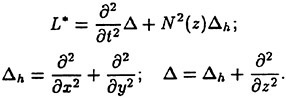
The initial condition is
(2)
The boundary conditions are stated at the upper surface, at the body depth and at the bottom. At the upper surface we assume the rigid lid condition
(3a)
This assumption means that we do not treat the surface wave field, but we retain the surface divergence/convergence effects because we have not assumed ∂W/∂z to be zero. At the bottom we have obviously
(3b)
where Η is the stratified layer thickness.
Consider the condition at the body horizon. The body shape is described by the two smooth functions h±: Z(x, y)=z0±h±(ξ, y), where ξ=x+Vt, z0 is the body depth, and the functions h± describe the body surfaces higher and lower than z0 respectively.
We assume the no-flow condition at the body surface:
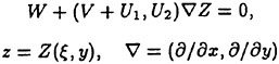
where U1, U2 are the velocity perturbations in the x and y directions, respectively. On the assumption that |h±(x, y)|≪1, U1,2≪1 this boundary
condition may be linearized with respect to h± and ∂h±/∂x and transferred to the depth z=z0 (6):
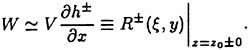
(3c)
This linearization assumes both h± and ∂h±/∂x to be small. If ∂h±/∂x is of the order of unity, then the perturbation velocity W is of the same order as the speed V and the linear model breaks down. The range of the applicability of this linearization is discussed in (6).
We seek the function W, which has a discontinuity
(4)
The solution of the problem (1)–(3a,b),(4) allows us to carry out the verification of the approximation (3c). For this purpose it is necessary to solve this problem numerically and then to draw calculated streamlines at z=z0. If the calculated fluid particle trajectories have qualitatively the same shape as that of the moving body, then this approximation is valid (Section 4.1).
A function W satisfying (1)–(3a,b) with the discontinuity (4) at z=z0 can be represented in the form
Here Ω is the domain and R(ξ, y) is not equal zero if (ξ, y) ∈ Ω. The function G(x, y, z, z0, t) describes the IW field vertical velocity generated by a point mass source which is switched on at t=0 and moves with the constant speed V at the depth z0 in the stratum −H<z<0. This function is a solution of the following problem
where δ(x) is Dirac function, Θ(t) is Heaviside function.
The limit of solution as t → ∞ for fixed ξ=x+Vt is the function G describing the vertical velocity of the stationary IW from a moving point mass source. This function is defined by the equations:
The vertical velocity W of stationary IW generated by a moving body is a solution of the following problem:
(5)
(6)
(7)
The solution of (5)–(7) is expressed in terms of the Green’s function as follows:
(8)
3. GREEN’S FUNCTION AND ITS ASYMPTOTICS.
The Green’s function G(ξ, y, z, z0) (where ξ=x+Vt) was obtained in (2) by the variable separation method in a form of a sum of modes:
(9)
where ![]() for ξ<0, and the functions are defined
for ξ<0, and the functions are defined ![]() by the integrals (2)1:
by the integrals (2)1:
(10)
(11)
with
(12)
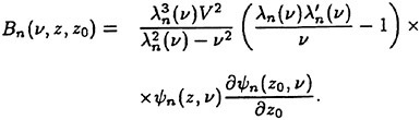
Here μn(ν), λn(ν) are odd functions ν, and ψn(z, ν), fn(z, ν) are even functions ν which are defined for ν>0 as eigenvalues and cigenfunctions of the corresponding spectral problems:
|
1 |
Analogous expressions in (4) contain misprints |
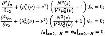
The same expressions are valid for the vertical displacement η excited by the moving point sourse (2) if we add factor signξ in the eqn. (10) and change ![]() by
by ![]() and
and ![]() by
by ![]() in the eqns. (12).
in the eqns. (12).
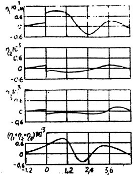
Fig. 1. First three modes of vertical displacement and their sum as functions of ξ.
Mention that in the case of vertical displacement each function ηn=Gn(ξ, y, z, z0) has a discontinuity at ξ=0 but this discontinuity must vanish after summing over n since the vertical displacement η=∑ηn is the analytic function ξ for y≠0. To illustrate it we present at taken from (2) Fig. 1 the first three modes of vertical displacement and their sum for H=600 m, distribution of N(z) shoved at Fig. 2, V=2 m/sec, y=300 m, z=200 m, and z0=22 m. We see, that each mode η1, η2, η3 is discontinuous, but their sum is continuous with graphical exactness. As was mentioned in (2), separate modes of vertical velocity are continuous at ξ=0.
The expressions (9)–(11) have the simple asymptotic forms close to and far from the point source.
In the near zone, i.e. for small y and ξ, the term ![]() makes the dominant contribution into G, and the terms
makes the dominant contribution into G, and the terms ![]() are relatively small. The series
are relatively small. The series ![]() is converging slowly, but it is possible to obtain the asymptotic form of
is converging slowly, but it is possible to obtain the asymptotic form of ![]() as n → ∞ (3):
as n → ∞ (3):
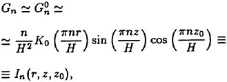
(13)
where r2=y2+ξ2, Ko(x) is the zeroth order MacDonald function (17). Each function In has a logarithmic singularity as r → 0 and z≠z0. The series ∑In can be summed (17):
(14)
Here z±=z±z0. The expression (14) is regular for r2+(z−z0)2≠0. It is the derivative with respect to z of the fundamental solution of Laplace equation: ΔI=−4πδ(z−z0)δ(ξ)δ(y) with boundary conditions I|z=0, −H=0. The sum (14) represents the field excited by a system of point sources placed at the depths zm=±z0±2mH, m=±0, 1,2,… in a non-stratified fluid.
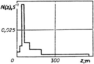
Fig. 2. Distribution of N(z)
We now write G in the form of a sum of a static field I and a rapidly converging series for small y, ξ:
(15)
At large distances from the point source G splits into individual modes with each mode propagating independently from the others within its own Mach angle (10,1,6). The terms ![]() make dominant contribution to G, since
make dominant contribution to G, since ![]() are exponentially small at large y. The asymptotical representation of Gn in the vicinity of the corresponding wave front is obtained from Taylor’s expansion of dispersion curves μn(ν) close to zero:
are exponentially small at large y. The asymptotical representation of Gn in the vicinity of the corresponding wave front is obtained from Taylor’s expansion of dispersion curves μn(ν) close to zero: ![]()
![]() and has the form (1):
and has the form (1):
(16)
where Ai′(x) is the first derivative of Airy function.
Far from each mode wave front and within its own Mach angle the asymptotical form of Gn is
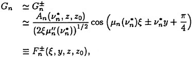
(17)
where ![]() is a root of the equation
is a root of the equation ![]() (1).
(1).
Thus, we have the following qualitative picture of the IW field at a fixed observation point located at a distance y from the source trajectory as t increases. For ξ=x+Vt<q1y the field at the observation point is exponentially small. For ![]() the front of the first vertical mode arrives at the observation point. In the vicinity of the front the field is expressed in terms of the Airy function derivative (16). Then, as ξ increases, i.e. for ξ>q1y, the field is expressed by (17). For
the front of the first vertical mode arrives at the observation point. In the vicinity of the front the field is expressed in terms of the Airy function derivative (16). Then, as ξ increases, i.e. for ξ>q1y, the field is expressed by (17). For ![]() the second vertical mode is joined to the field, for
the second vertical mode is joined to the field, for ![]() the third mode is joined to the field, etc.
the third mode is joined to the field, etc.
4. EXAMPLES OF CALCULATIONS AND ALGORITHMS.
There are three regions of IW field. The points in the near zone are separated form the body at the distances comparable to the thickness Η. Here the field is practically independent of the stratification, and IW amplitudes are the biggest. For the points in the far zone y, ξ≥10 H. In this zone IW field splits into individual modes, each mode is situated within corresponding Mach angle and the amplitude of the mode is small outside its Mach angle. Finally, there is an intermediate zone, where the IW field structure is more complicated. The code chooses the algorithm of field calculation in dependence of position of observation point with respect to body.
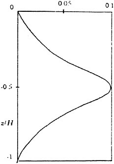
Fig. 3. The distribution of the Brünt-Väissälä frequency N(z).
The work of code begins from numerical calculation of dispersion curves μn(ν), λn(ν), and eigenfunctions fn(z, ν), ψ(z, ν) for given density distribution and prescribed values n. These results are used during all subsequent calculations.
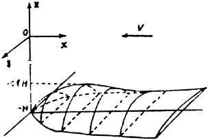
Fig. 4. The shape of body.
For depicted below and taken from (4) examples of calculations we choosed the model of moving body and the stratification of fluid which were used for calculations in (6). In this model the depth of body is equal to the thickness Η=50 m of the stratified layer, maximal height of body h*=0.2 H; its velocity V=5 m/sec. The distribution of Brünt-Väissälä frequency N(z) is shown at Fig. 3 and the shape of body is shown at Fig. 4.
Some results of numerical calculations are shown at Figs. 5, 6. At Fig. 5 is depicted the vertical
velocity W as function ξ for y=0 and different values of z. Note that our results practically coincide with results of (6); the vertical velocity rapidly decreases and perturbed region expands with decrasing depth z. The amplitude of W at z=−0.5 H is only 15% of its values at z=−H which coincides with the function R(ξ, y).
At Fig. 6 is shown the vertical displacement η as function y, ξ for z=−0.5 H.
Let us present now the algorithms of field calculation.
4.1 Field in the near zone. It is convenient to use here the representation of Green’s function in the form (15). For W we obtain:
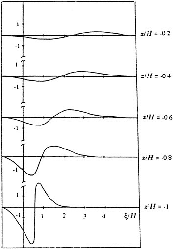
Fig. 5. Vertical velocity W at different depth and y=0.
(18)
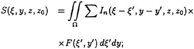
(19)
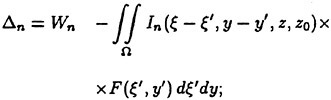
where Wn is the exact integral representation of the individual mode (Section 4.3).
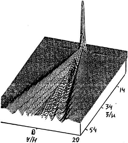
Fig. 6. Vertical displacement n for z=−0.5 H.
The function S satisfies the Laplace equation ΔS=0 and the boundary conditions (6)–(7), i.e., describes the flow of the nonstratified fluid around the body. To calculate S we use eqn. (14) for ∑In. As the numerical calculations show, at the distance of the order of H from the body, the flow is almost potential and depends only on the body shape.
However, as the distance from the body increases, it becomes necessary to take into account the fluid stratification. Then a procedure for calculating the corrections to the potential flow at the point ξ, y, z in order to take stratification into account is as follows: (1) the function S is calculated from (18); (2) the term Δ1 is determined, if |Δ1|≪|S| then next terms in (18) need not be found; (3) if |Δ1| and |S| are of the same order, then the term Δ2 is calculated; (4) if |S+Δ1|≫|Δ2| then the summation in (18) is interrupted, and so on.
The procedure described makes it possible not only to calculate the IW near field accurately, but also to estimate the errors in the asymptotic expressions. At Fig. 7 are depicted for y=0.5 H, z=−0.5 H the exact value W of vertical velocity and the functions S, S Δ1, S+Δ1+Δ2. These results show that at the distances from trajectory of the order of thickness Η in is suffitient to take into account only two corrections.
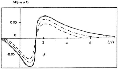
Fig. 7. Vertical velocity in near zone y=0.5 H, z=−0.5 H: exact solution W (solid line), functions S (dashed line), S+Δ1 (dot-and dashed line), S+Δ1+Δ2 (dotted line).
The trajectories of fluid particles for z=z0 calculated for our model are close with sufficient accuracy to the prescribed shape of moving body. It confirms the validity of linear approximation (3c) for the boundary conditions.
4.2 Field in the far zone. As was mentioned above, at large distances from the moving body the IW field splits into individual modes. Moreover, it is possible to show from (15)–(17) that only the longwave components are essential at these distances (1).
So, we disregard the exact body shape and replace it by a suitable system of point sources. For the present case the function R(ξ, y) can be written approximately in the form
(20)
where coordinates of the source ξ+, sink ξ− and constant R* are determined by the body shape.
Then, using the asymptotic representations of Green’s function (16),(17), we can write the expression for the individual mode Wn in the far zone:
(21)
The results of calculations in accordance with (21) for intermediate (y=2 H) and far (y=8 H) zones are shown at Fig. 8. Numerical estimations show that in far zone (for y>10 Η) the use of the asymptotic of the Green function and replacement of body by a suitable system “source+sink” maked it possible to calculate IW field by simple explicit expressions instead of numerical calculation of the exact integrals.
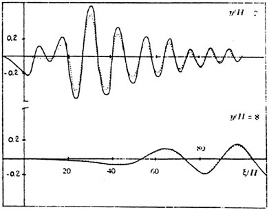
Fig. 8. The first mode of vertical velocity for z=−0.5 H in intermediate (y=2 H) and far (y=8 H) zones: exact mode W1 (solid lines), approximation (21) (dotted lines).
4.3 Field in the intermediate zone. In order to simplify the exact calculations in intermediate zone we consider here the body shape with vertical cross-section orthogonal to the x axis in the form of a semi-ellipse (6):
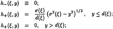
where arbitrary smooth functions σ(ξ), d(ξ) describe the height and the width of the body cross-section. In this case, using (9)–(11), it is possible to integrate in (8) over y and to obtain the expression for W in the form:
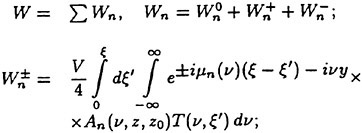
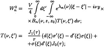
where τ=νd(ξ)/2, J0,1(x) are the zeroth and the first order Bessel functions.
ACKNOWLEDGEMENTS.
The results described above were made possible in part by grant N M31000 from the International Science Foundation.
References
[1] Borovikov, V.A., Vladimirov, Yu.V. and Kel’bert, M.Ya. Field of internal gravity waves excited by localized sources. Izv.Atm.Ocean.Phys., No. 6, 1984, pp. 494–498.
[2] Borovikov, V.A., Bulatov, V.V., Vladimirov, Yu.V. and Levchenko, E.S. Internal wave field generated by a source resting in a moving stratified fluid. J.Appl.Mech.Tech.Phys., No. 4, 1989. pp. 563–566.
[3] Bulatov, V .V. and Vladimirov, Yu.V. Near field of internal waves exci0ted by a source in a moving stratified liquid. J.Appl.Mech.Tech.Phys., No. 1, 1991. pp. 21–25.
[4] Borovikov,V.A., Bulatov, V.V., and Vladimirov, Yu.V. Internal gravity waves excited by a body moving in a stratified fluid. Fluid Dynamics Research, 1995, Vol. 15, pp. 325–336.
[5] Hopfinger, E.J. Turbulence in stratified fluids: a review. J.Geophys.Res., Vol. 92, 1987. pp. 5287–5303;
[6] Kallen, E. Surface effects of vertically propagating waves in stratified fluid. J.Fluid Mech., Vol. 182, 1987. pp. 111–125.
[7] Lin, J.-T. and Pao, Y.-H. Wakes in stratified fluids. Ann.Rev.Fluid Mech., Vol. 11, 1979. pp. 317–338.
[8] Sharman, R.D. and Wurtele, M.G. Ship waves and Lee waves. J.Atmosph.Sci., Vol. 40, 1983. pp. 396–427.
[9] Miles, J.W. Internal waves, generated by a horizontally moving source. Geoph.Fluid Dyn., Vol. 2, 1971. pp. 63–87.
[10] Keller, J.B. and Munk,W.H. Internal wave wakes of a body moving in a stratified fluid. Phys.Fluids, Vol. 13, 1970. pp. 1425–1431.
[11] Janowitz, G.S. Lee waves in three-dimensional stratified flow. J.Fluid Mech., Vol. 148, 1984. pp. 97–108.
[12] Meng, J.C.S. and Rottman, J.W. Linear internal waves generated by density and velocity perturbations in a linearly stratified fluid. J.Fluid Mech., Vol. 186, 1988. pp. 419–444.
[13] Voisin, B. Internal wave generation in uniformly stratified fluid. Part 1. Green’s function and point sources. J.Fluid Mech., Vol. 231, 1991. pp. 439–480.
[14] Gray, E.P., Hart, R.W. and Farrel, R.A. 1983. The structure of the internal wave Mach front generated by a point source moving in a stratified fluid. Phys.Fluids, Vol. 26, 1983. pp. 2919–2931.
[15] Snyder, W.H., Thompson, R.S., Eskridge, R.E., et al. The structure of strongly stratified flow over hills dividing-streamline concept. J.Fluid Mech., 152, 1985. pp. 249–289.
[16] Gill, A.E. Atmosphere-Ocean Dynamics, Academic Press, 1982.
[17] Gradstein, I.S. and Ryshik, I.M. Tables of Integrals, Series and Products. Academic Press, 1980.
DISCUSSION
I.Sturova
Lavrentyev Institute of Hydrodynamics, Russia
The given report is devoted to the important problem of internal gravity wave generation in a stratified fluid resulting from the horizontal motion of a submerged body and its associated turbulent wake. Unfortunately, at present there is no definite understanding of all the sources responsible for a generation of internal waves by a towed or self-propelled body. Models used in the 70s and 80s are under reconsideration at the present time (see e.g. (1)) especially at high speed of body motion.
The authors used the model proposed by Kallen (2), where a body together with a turbulent wake is modeled by an infinitely long thin body. Despite the disputability of the model used, the undoubted advantage of the given paper is the proposed effective method of determination of the Green function of a point mass source moving uniformly in a fluid with an arbitrary stable stratification. The asymptotic estimations for near and far field are obtained.
To my point of view, this method will be extremely useful for computation of the flow around the moving solid body of an arbitrary form with a non-flow condition at the body’s surface. Analogously to the computation of the flow around a body submerged under the free surface of homogeneous fluid, it is possible to use the boundary element method demanding a determination of the Green function for the problem and work out of algorithm of its effective calculation. If the problem is solved successfully together with the determination of wave field, the effect of stratification on hydrodynamics loads acting on a body can be estimated.
References
1. Robey, H.F., “The Generation of Internal Waves by a Towed Sphere and Its Wake in a Thermocline,” Physics of Fluids, Vol. 9, No. 11, 1997, pp. 3353–3367.
2. Kallen, E., “Surface Effects of Vertically Propagating Waves in Stratified Fluid,” Journal of Fluid Mechanics, Vol. 182, 1987, pp. 111–125.
AUTHORS’ REPLY
The authors agree with the discusser’s comments.


