
Projected Supply of Cellulosic Biomass
The consumption mandate for two of the four categories of biofuels listed in the Renewable Fuel Standard as amended by the Energy Independence and Security Act (EISA) of 2007 (RFS2) will likely be met by corn-grain ethanol and biodiesel, as discussed in Chapter 2. The remaining 20 billion gallons per year of mandated consumption is to be met with cellulosic biofuels or advanced fuels, which could include cellulosic biofuels, other types of biofuels derived from sugar or any starch other than corn starch, and imports of ethanol from sugarcane facilities in Brazil and elsewhere. Based on anticipated advances in conversion technologies, earlier studies suggested that over 550 million dry tons per year of nonfood-based resources, including agricultural residues, dedicated bioenergy crops, forest resources, and municipal solid wastes (MSWs), can potentially be produced in the United States (Perlack et al., 2005; NAS-NAE-NRC, 2009). However, the potentially available feedstock that would be supplied to biofuel refineries in the future depends on multiple factors: where the feedstock is grown and collected; expected crop, residue, or forest yields; competition for biomass from other uses (for example, electricity generation versus biofuel production); markets; technology development; public policies; and other unanticipated factors. Potential availability refers to the amount of cellulosic biomass that could be grown and harvested in the United States based on assumptions of recoverable yields from diverse farm and forest landscapes but without specific consideration of the costs of producing, harvesting, and delivering the biomass to a biorefinery. The study Biomass as Feedstock for a Bioenergy and Bioproducts Industry: The Technical Feasibility of a Billion-Ton Annual Supply1 (Perlack et al., 2005) provided one of the first estimates of potential availability of cellulosic feedstocks in the United States. Supply refers to a schedule of amounts that would be delivered to biorefineries at different costs, taking accessibility of biomass, infrastructure, and other
______________
1 The report U.S. Billion-Ton Update: Biomass Supply for a Bioenergy and Bioproducts Industry (Perlack and Stokes, 2011) was released while the committee was preparing this report for public release. The committee did not have an opportunity to review the Perlack and Stokes (2011) report.
economic conditions into consideration. Taking all those factors into consideration, realized supply is likely to be much lower than potential availability.
This chapter describes the estimated supply of cellulosic biomass made by different groups, including the researchers at the University of California, Davis, the U.S. Environmental Protection Agency (EPA), the Biomass Research and Development Initiative, and researchers at the University of Tennessee. Other factors, such as biotechnology, competition for biomass with other sectors, weather-related losses, and pests and diseases, which are typically not considered in projecting biomass supply, contribute to uncertainties in feedstock supply and are discussed at the end of this chapter.
POTENTIAL SUPPLY OF BIOFUEL FEEDSTOCK AND LOCATION OF BIOREFINERIES
Several studies attempted to predict the most likely locations for biomass production and corresponding siting of the biofuel biorefineries for regulatory and other planning purposes (BRDB, 2008; English et al., 2010; EPA, 2010; Parker et al., 2010b; USDA, 2010). Some studies principally identify the regional availability of bioenergy feedstocks that could be used for biofuel production, while others also identify likely biorefinery locations. The following sections describe some of the approaches and assumptions used in the modeling of potential feedstock supply and biorefinery locations and compare projected locations for biorefineries among studies and with some of the proposed locations of cellulosic biofuel refineries. A comparison of the assumptions related to the types and amounts of feedstocks and the conversion rate to energy is provided in Table 3-1.
National Biorefinery Siting Model
Approach and Assumptions
The National Biorefinery Siting Model (NBSM) was developed by researchers at the University of California, Davis (Parker et al., 2010a; Tittmann et al., 2010; Parker, 2011). It integrates geographically explicit biomass resource assessments, engineering and economic models of the conversion technologies, models for multimodal transportation of feedstock and fuels based on existing transportation networks, and a supply chain optimization model that locates and supplies a biorefinery based on inputs from the other models (Parker et al., 2010a). To identify the location of biorefineries, the model first maximizes the profitability of the entire national biofuel industry. The profit maximized is the sum of the profits for each individual feedstock supplier and fuel producer. Costs minimized in the model are those associated with feedstock procurement, transportation, conversion to fuel, and fuel transmission to distribution terminals. Fuel production and selling price determine industry revenue. Coproduct revenues are included.
NBSM used data from the U.S. Department of Agriculture (USDA) National Agricultural Statistics Service (NASS) and Forest Service (USFS) provided by Skog et al. (2006, 2008) to project crop and woody biomass location and abundance and create spatially explicit estimates of biomass availability. NBSM constrained estimates for the supply of corn to be equal to the quantity needed to meet the RFS2 mandate of 15 billion gallons per year for conventional ethanol. Soybean and canola were assumed to be grown and used for biofuels. To limit the proportion of soybean dedicated to fuel production in the model, the use of soybean oil for biodiesel is limited to not more than 38 percent of all soy oil produced.
TABLE 3-1 Comparison of Assumptions in Biomass Supply Analyses
| Cellulosic Feedstocks | Other Feedstocks | Biomass Supply in 2022 | Energy Conversion Ratio | |
| National Biorefinery Siting Model | Corn stover Switchgrass Woody biomass | Greases MSW |
500 million dry tons of all feedstock types | Varies by technology and feedstock type |
| EPA | Corn stover Switchgrass Other dedicated bioenergy crops Bagasse Sweet sorghum pulp Woody biomass |
MSW | 82 million dry tons of corn stover in 2022 10 million dry tons of bagasse 44 million dry tons of woody biomass |
Over 90 gallons per dry ton, but varies by feedstock 94 gallons per dry ton for corn stover in 2022 |
| USDA | Logging residue Dedicated bioenergy grasses Soybean Energy cane Sweet sorghum Canola Corn stover Straw |
NA | 42.5 million dry tons of logging residue | 70 gallons per dry ton of logging residue Conversion ratios for other feedstocks not included in source |
| Biomass Research and Development Initiative | Corn stover Wheat straw Dedicated energy crops, including switchgrass Woody biomass including hybrid poplar and willow Sweet sorghum | NA | 75-79 million dry tons of dedicated energy crops and annual energy crops like sweet sorghum in 2022 45 million dry tons of woody biomass in 2022 51-84 million dry tons of corn stover in 2022 20-32 million dry tons of wheat straw in 2022 | 80-90 gallons of ethanol per dry ton of switchgrass Conversion ratios for other feedstocks not included in source |
NOTE: All analyses assumed that the 15-billion gallon mandate for conventional biofuel would be met by corn-grain ethanol.
NBSM also constrains cellulosic feedstock acquisition from all sources to an area within a 100-mile radius of the biorefinery site for the most part. Crop residue removal was constrained to levels that were estimated to prevent erosion. Those levels were estimated using local soil and landscape data and methods to estimate effects on soil quality and erosion (Nelson, 2002; Nelson et al., 2004, 2006). A combination of soil erosion (by wind and water) models were used to estimate the upper limit of crop residue removal. An amount of residue lower than the upper limit is considered to be removable without detrimental effects on the environment and resource base. The methods used combine detailed field-scale data on soil type, capability class, and slope from the USDA Natural Resources Conservation Service (NRCS) Soil Survey Geographic (SSURGO) database (USDA-NRCS, 2008) and an estimation of maximum rate of soil erosion not affecting productivity (the T value calculated using the Universal Soil Loss Equation; Renard et al., 1997). Residue amounts come from crop yields derived from the NASS database cited above. Wind erosion limits are
also calculated using methods described by Nelson (2002). A limitation of these methods is that they do not account for some aspects of soil management, such as soil organic matter (SOM) maintenance. They do not include estimates of technical limits to stover recovery. Removal rates could be overestimated if the amount of stover left on the field is less than the amount needed to conserve SOM.
Switchgrass is modeled based on yields estimated at the Oak Ridge National Laboratory (Jager et al., 2010) using results from a survey of the most current agronomic literature and predictions from a switchgrass model developed by the Pacific Northwest National Laboratory (Thomson et al., 2009). Harvest costs are estimated using a model from the Idaho National Lab (Hess et al., 2009). Residue and cellulosic yield and cost estimates are resolved to the county level and calculated as an edge of field price. Costs and supply estimates are derived from the Policy Analysis System (POLYSYS) modeling framework (Walsh et al., 2003). POLYSYS estimated switchgrass to be available at $50 to $85 per dry ton, at the farm gate.
Estimates of forest biomass to the county level were derived from several sources. Accessible biomass estimates were guided by sustainability principles. However, the sustainability guidelines are site specific or region specific and could vary by ownership, with federal rules and guidelines, state guidelines, or professional standards used to guide management and harvest. In all cases, forest biomass generally included is the secondary output of other commercial forestry operations. Therefore, significant variability and uncertainty about resource access exists. Forest biomass available for biofuel production was estimated for the thinning of timberland with high fire hazard, logging residue left behind after anticipated logging operations for conventional products, treatment of Pinyon Juniper woodland and rangeland, normal thinning of private timberland, precommercial thinning on National Forest land in western Oregon and Washington, and unused mill residue.
EISA excludes credit for wood removed from federal lands, so NBSM provides separate estimates of forest biomass availability with and without federal lands. Forest resources were estimated to be available starting at $20-$30 per dry ton at the roadside, with the majority available at $45-$65 per dry ton, all depending on location, at the time of simulation. Pulpwood is available to biorefineries at suitable locations at up to $100 per dry ton. In addition to USFS data sources already noted, various models were used to estimate amounts available and costs for biomass harvest and removal (Biesecker and Fight, 2006).
Biorefineries are sited in or near cities in NBSM. No water constraints on biorefinery operation are assumed in the model for this reason. Water availability could limit the number of new refineries using cellulosic biomass in some regions, and this might be true for some existing corn-grain ethanol refineries as well (NRC, 2008). Corn-grain ethanol production is modeled using current information on ethanol refinery location, size, and cost. Optimistically, biorefineries are considered to be able to use mixed feedstocks for the most part. Where mixed feedstocks are available, corn-grain ethanol is produced up to the limit imposed by RFS2, and then crop residues, dedicated bioenergy crops, fats, oils and greases, and MSW all contribute to biofuel supply, with the mixtures varying locally.
Two conversion technologies are represented in the model: biochemical fermentation of ethanol from grain and cellulosic feedstocks and thermochemical production of biofuels from mostly cellulosic feedstocks. The use and costs of dilute acid hydrolysis followed by ethanol production from fermentation is modeled for lignocellulosic feedstocks. Although several thermochemical pathways could be used to convert cellulosic biomass to fuels (see Chapter 2), gasification followed by Fischer-Tropsch synthesis was used in NBSM to represent a larger class of thermochemical processes, including pyrolysis and other gasification
technologies, that create biomass-derived diesel. Optimal combinations of feedstocks and technologies vary regionally. However, each simulation provides results of national or industry-wide fuel production at a given fuel price and identifies optimal locations and size of biorefineries and types of biomass resources used at each biorefinery. The selling prices of the product fuels are input parameters that are varied to create a supply curve through multiple model iterations across a range of prices ($1.00-$5.50 per gallon of gasoline equivalent) (Figure 3-1).
Results
The model predicted that the RFS2 consumption mandate of 36 billion gallons of biofuels by 2022 can be met at $2.90 per gallon of gasoline equivalent (or $1.91 per gallon of ethanol) at the time the most recent simulations were conducted (Figure 3-1). At this price, about 500 million dry tons of different types of biomass (including corn grain, fats, and oil) would be converted to biofuels nationally. Of the 500 million dry tons of biomass, 360 million are cellulosic biomass. The committee cautions that the estimated prices for various cellulosic feedstocks in NBSM are lower than the more recent estimates presented in
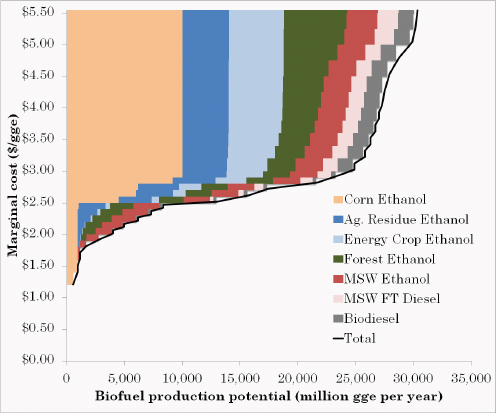
FIGURE 3-1 Biofuel supply and fuel pathways estimated from teh National Biorefinery Siting Model.
NOTE: About 500-600 million dry tons per year of biomass are considered available and recoverable at prices needed to meet RFS2 in 2022. Feedstock use reflects availability and price.
SOURCE: Jenkins (2010). Reprinted with permission from N.C. Parker, University of California, Davis.
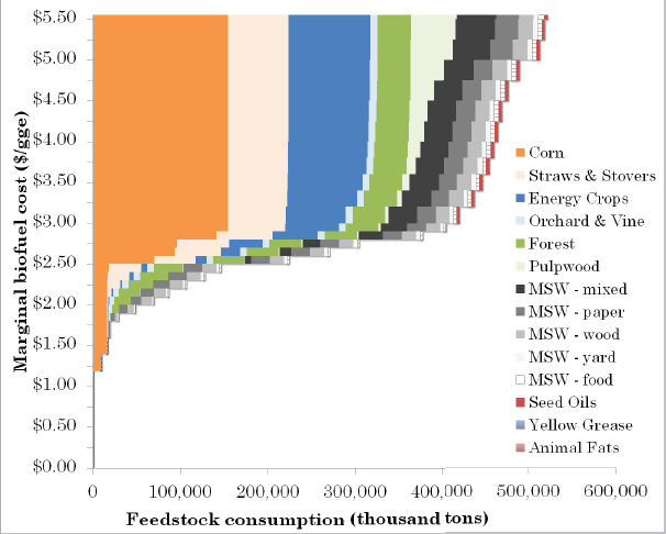
FIGURE 3-2 Biomass supply curves estimated by the National Biorefinery Siting Model.
SOURCE: Jenkins (2010). Reprinted with permission from N.C. Parker, University of California, Davis.
Chapter 4 of this report. The estimates of feedstock costs used in NBSM are at the farm gate and do not include the opportunity cost of cropland.2 Although delivery costs were not included as part of feedstock costs, NBSM accounts for the cost of feedstock transport to biorefinery in its analysis.
Types and amounts of biomass vary with biofuel cost (Figure 3-2 and Table 3-2). The range and quantities of potential feedstocks increase with higher biofuel costs. As can be expected, agricultural residues are concentrated in the Corn Belt (Figure 3-3A). The areas with the highest yield per acre for perennial herbaceous grasses are not the areas with the largest supply (Figure 3-3B). The area with the highest quantity of forest residue is the Pacific Northwest followed by the Southeast (Figure 3-3C). As discussed in Chapter 2, models projecting yield on the basis of agronomic conditions suggest that Miscanthus and switchgrass are most productive on existing cropland. Because NBSM maximizes profitability of land use and commodity crops have higher value than perennial
______________
2 Opportunity cost is the net returns forgone by the producer for not using cropland to produce the next-best (or next most profitable) crop or product.
| MSW | Feedstock Type (in thousands of dry tons per year) | |||||||
| Region | Biorefinery Locations | Forest | Pulpwood | Corn Grair | Crop Residues | Dedicated Bioenergy Crops |
Orchard and Vineyard Wastes | |
| North Central and Northeast |
Grayling, MI | 338 | 8.1 | 17.5 | ||||
| Warren, MI | 541 | 123 | ||||||
| Port Huron, MI | 500 | |||||||
| Saginaw, MI | 500 | 636 | 268 | |||||
| Marquette, WI | 194 | 2.3 | ||||||
| Rhinelander, WI | 502 | |||||||
| Bemidji, MN | 289 | |||||||
| Syracuse, NY | 20.8 | 268 | 1,000 | 30.8 | 595 | 60.9 |
||
| Mid-south | Fayetteville, AR | 29 | 301 | 23.4 | 13 | 600 | 23.6 | |
| Poplar Bluff, MO | 282 | 527 | ||||||
| Paducah, KY | 147 | 865 | ||||||
| Jackson, TN | 63.1 | 1,240 | ||||||
| Memphis, TN | 12,800 | 881 | 479 | |||||
| Morristown, TN | 1,120 | |||||||
| Murfreesboro, TN | 4.8 | 1,050 | |
|||||
| Southeast | Huntsville, AL | 4.8 | 811 | |||||
| Greenville, MS | 1,000 | 836 | 306 | |||||
| Vicksburg, MS | 540 | |||||||
| Columbus, MS | 28.2 | 538 | 58.3 | 1.3 | ||||
| Waycross, GA | 730 | 275 | 42.6 | |||||
| Greenwood, SC | 4.1 | 797 | ||||||
| Asheville, NC | 52.6 | 630 | 29.7 | 17.2 | ||||
| Fayetteville, NC | 600 | |||||||
| Lumberton, NC | 36.2 | 646 | 104 | |||||
| Danville, VA | 75.8 | 496 | 34.7 | 22.1 | 1,300 | |||
| MSW | Feedstock Type (in thousands of dry tons per year) | |||||||
| Region | Biorefinery Locations | Forest | Pulpwood | Corn Grair | Crop Residues | Dedicated Bioenergy Crops |
Orchard and Vineyard Wastes | |
| Northern Plains | Nebraska City, NE | 444 | 344 | |||||
| Norfolk, NE | 2,070 | 11,100 | 241 | |||||
| Howard, SD | 1,000 | 526 | 706 | |||||
| Pierre, SD | 80.8 | 790 | ||||||
| Sioux Falls, SD | 1,210 | 1,260 | 95.8 | |||||
| Watertown, SD | 1,000 | 989 | 371 | |||||
| Jamestown, SD | 1,000 | 132 | 379 | |
||||
| Southern Plains | Garden City, KS | 684 | 18.6 | 910 | ||||
| Guymon, OK | 94.8 | 770 | ||||||
| Keys, OK | 1,030 | |||||||
| Dumas, TX | 1,000 | 139 | 1,120 | |||||
| Hereford, TX | 115 | 113 | 931 | |||||
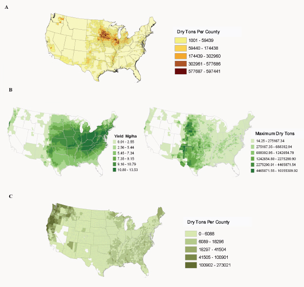
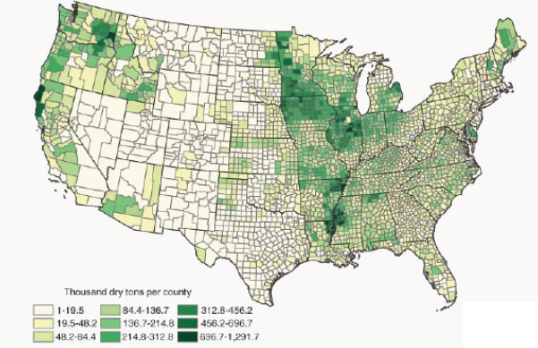
A. Agricultural residue availability (dry tons per county).
B. Energy crop yields (Mg per hectare) and projections of maximum available supplies (maximum dry tons).
C. Estimated forest residue on public and private land (dry tons per county).
NOTE: Figure 3-3C also includes forest residues from federal forestland that do not qualify as renewable biomass under EISA’s definition.
SOURCE: Jenkins (2010). Reprinted with permission from N.C. Parker, University of California, Davis.
herbaceous energy crops, the model estimated the perennial herbaceous energy crops would be planted on less productive lands. The projected distribution of crop residue, switchgrass, and Miscanthus supplies are consistent with another study that projects national cellulosic biomass supply using a multimarket equilibrium nonlinear mathematical programming model called the Biofuel and Environmental Policy Analysis Model (Khanna et al., 2011) and a study that projects regional cellulosic biomass supply in Michigan (Egbendewe-Mondzozo et al., 2010). Most of the supplies of woody biomass are projected to come from the north central and southeastern parts of United States. Biorefinery sites and the associated feedstock sheds identified by the model nationally are presented in Figure 3-4.
SOURCE: Jenkins (2010). Reprinted with permission from N.C. Parker, University of California, Davis.
EPA
Approach and Assumptions
In its Regulatory Impact Analysis (EPA, 2010) for RFS2, EPA describes a transport tool that estimates the location of cellulosic biorefineries to be built to produce 16 billion gallons of cellulosic biofuels by 2022. Biomass data were derived from a number of sources, including NASS for agricultural residues, Elliot Campbell from Stanford University for bioenergy crops, and the U.S. Forest Service for forestry residue. MSW also was included as a potential feedstock for biofuels.
For each U.S. county, feedstock availability is estimated from the Forest and Agricultural Sector Optimization Model (FASOM, as discussed in Appendix K). FASOM was modified to reflect the current RFS2 program to include updated values for herbaceous energy crop yields, cellulosic ethanol conversions, and modifications to the accounting procedures for rangeland (Beach and McCarl, 2010). Switchgrass yields used in FASOM were derived from Thompson et al. (2009). Crop yields were projected to increase at current rates. The conversion yield from biomass to ethanol was assumed to be 90-94 gallons per dry ton depending on the feedstock (EPA, 2010).
The EPA siting tool also estimated cost information for each feedstock available. These costs included the roadside cost of production, transportation to move the feedstock to the centroid of its own county or from a neighboring county, and the secondary storage of that feedstock. Each county data point contains a list detailing the total cost of each feedstock available in that county. This list of feedstock availability and costs is used to choose feedstocks that a centrally located biorefinery would process. A biorefinery is assumed to process multiple feedstocks if they are available in the area. For each county, the cheapest feedstocks are selected for the biorefinery, and the volume of feedstock available at this price was converted to gallons, based on feedstock conversion modeled by FASOM (Tao and Aden, 2008), and added to a running count of the total volume of feedstock processed by that county, up to a maximum processing volume. Feedstock prices and conversion are reported by Beach and McCarl (2010). Biorefineries are assumed to be 100 million gallons per year in capacity, based on assumptions from FASOM and Carolan et al. (2007).
Capital costs associated with the increased volume were added to the total cost of the feedstock processing for that county. The model selected feedstock sources using a cost minimization algorithm that selects progressively more expensive feedstocks until the county either reaches a set 90-percent maximum processing volume or if adding another feedstock would produce a more expensive result on a price per gallon basis. At the end of this step, each potential county biorefinery location contained information regarding the cheapest total cost to produce cellulosic ethanol at that location. The most competitive locations were identified by comparing feedstock and capital costs. These locations resulted in a list of estimated least-cost biorefinery locations needed to meet 16 billion gallons per year mandated cellulosic biofuels. (The 4 billion gallons per year of advanced biofuels, which could be met by imports, were not included in this analysis.) The EPA Transport Tool does not take availability of water, permits, or human resources into account.
Results
The EPA Transport Tool estimated the majority of cellulosic biorefineries to be located in the upper Midwest and the Southeastern states (Figure 3-5). Because the tool projected
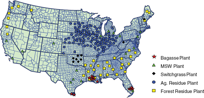
FIGURE 3-5 Locations of cellulosic facilities projected by the EPA Transport Tool.
SOURCE: EPA (2010).
biorefinery locations on the basis of price and the ease of recovery, corn stover would be the primary feedstock for cellulosic ethanol in 2022 (EPA, 2010; Table 1.8-13, p, 275). About 380 million dry tons of corn stover3 were estimated to be available, of which 82 million dry tons could be supplied for producing 8 billion gallons of ethanol. Additional cellulosic biofuels were predicted to come from other crop residues in Florida, Texas, and Louisiana (primarily 10 million dry tons of bagasse associated with sugarcane harvest) and from dedicated bioenergy crops (primarily switchgrass) in the Southeastern states. Straw from wheat harvest in the Midwest or elsewhere was not included in EPA’s model. Forestry residues also were considered likely feedstocks, primarily in the Southeastern United States and in a few locations in the Northwest and the Northeast (EPA, 2010). EPA estimated 44 million dry tons of woody biomass would be converted to biofuel in 2022.
USDA
Approach and Assumptions
USDA published the report A USDA Regional Roadmap to Meeting the Biofuels Goals of the Renewable Fuels Standard by 2020 (USDA, 2010) to provide an overview of that agency’s estimates for biofuel production by macro-region and biomass types. The report assumes that corn-grain ethanol production will meet the 15 billion gallons per year target for conventional fuels in 2020. The analysis in the report focuses on one scenario in which U.S. agriculture could produce enough biomass feedstock for biofuels to meet the remaining 21 billion gallons of biomass-based diesel, advanced biofuels, and cellulosic biofuels in the consumption mandate. USDA’s analysis included corn stover, straw, soybean, canola, sweet sorghum, sugarcane for energy production, perennial grasses for energy production, and logging residue. It did not include MSW, algae, or manure as feedstocks. Energy conversion yields were calculated for each feedstock, but only the ethanol yield of logging residue was reported. This yield was assumed to be 70 gallons per dry ton, and residue availability was limited to recoverable amounts from permitted timber harvests on federal, state, and private lands as estimated by the U.S. Forest Service. The report is based on a synthesis of the professional judgment of scientists from the USDA Agricultural Research Service. Many details of assumptions used were not provided.
Results
The USDA report concluded that 27 million acres of cropland, representing 6.5 percent of all U.S. cropland, would be needed to produce enough biomass feedstock to meet RFS2. The amount of biomass supplied from that land was not reported, with one exception. The report estimated that 42.5 million dry tons of logging residues that are not used for any other purposes would be available for biofuel production in 2022. That estimate was based on actual data from the 2001-2005 period.
The Southeastern and Middle Atlantic states were estimated to provide the largest amount (10.5 billion gallons per year) of biofuels needed to meet the RFS2 mandate from dedicated bioenergy crops, soybean, energy cane, sweet sorghum, and logging residues. USDA attributed the high potential for biofuel production in this region to its robust growing season and estimated yield advantages of energy crops compared to corn. The Corn Belt
______________
3 In its calculation, EPA assumed a 1:1 of stover to grain. However, it did not account for the fact that corn grain contains 15 percent moisture. Thus, 1 dry ton of corn grain would yield about 0.85 dry ton of stover.
and surrounding states (central east) were estimated as the second largest source of feedstock for biofuels (9.09 billion gallons per year) with dedicated bioenergy crops, canola, soybean, sweet sorghum, corn stover, and logging residues as the principal feedstock sources. For the most part, USDA estimated little crop substitution in the most productive regions of the Corn Belt. Other regions of the United States are estimated to provide only small portions of the mandated fuels (Table 3-3).
Biomass Research and Development Initiative
Approach and Assessment
The Biomass Research and Development Board (BRDB) was established to coordinate federal research and development activities associated with biofuels, biopower, and bioproducts. The Biomass Research and Development Initiative was legislatively directed to address “feedstocks development, biofuels and biobased products development, and biofuels development analysis” (BRDB, 2010). BRDB released the report Increasing Feedstock Production for Biofuels: Economic Drivers, Environmental Implication, and the Role of Research (BRDB, 2008) that included modeling feedstock supply and distribution on the basis of the Regional Environment and Agriculture Programming (REAP) model (Johansson et al., 2007) linked to POLYSYS (described below and in Appendix K). The study focuses on the biofuel feedstocks needed to meet the EISA 2007 mandates. It used the REAP model to predict corn-grain ethanol production under a range of assumptions about technology development, crop yield, and oil supply. However, POLYSYS was used to simulate production of cellulosic feedstock because REAP does not have the capability to assess dedicated energy crops or the collection of crop residues. Three scenarios with varying contributions were presented. First, 20 billion gallons of advanced and cellulosic biofuels would be produced from cellulosic feedstock (corn stover, wheat straw, dedicated energy crops including switchgrass, and sweet sorghum) from U.S. cropland only. The committee judged the first scenario as unlikely because of the extent of land changes that would be incurred. The second scenario assumes that 16 billion gallons of biofuels would be produced from cellulosic feedstock from U.S. cropland and 4 billion gallons of biofuels would be from forest resources (such as hybrid poplar and willow). The third scenario assumed that all 4 billion gallons of advanced biofuels would be met by imports and the remaining 16 billion gallons of cellulosic biofuels would be produced from cropland and forest resources. As in the case of POLYSYS (discussed later in this chapter), that BRDB report used published data on yields and prices as a baseline and predicts changes from that baseline.
Results
Under the two scenarios, the BRDB estimated that 51-84 million dry tons of corn stover, 20-32 million dry tons of wheat straw, 45 million dry tons of woody biomass, and 75-79 million dry tons of dedicated perennial (such as switchgrass) and annual (such as sweet sorghum) energy crops could be supplied to meet the mandate in 2022. Switchgrass was estimated to yield 80-90 gallons of ethanol per ton. Energy conversion yields for other feedstocks were not provided.
Results from the BRDB study emphasized the importance of crop yield assumptions for land use and biomass feedstock production. Under various scenarios, the BRDB report predicted that most dedicated bioenergy crop production will be derived from the lower Mississippi Valley and Delta region, the Southeastern coastal plains and Gulf slope regions, and
| Region | States Within Region | Feedstock Type Available (In Order of Importance) | Volume of Ethanol Produced from Feedstock (billon gallons per year) | Volume of Biodiesel Produced from Feedstock (billion gallons per year) | Total Volume (billion gallons per year of ethanol equivalent) |
| Southeast and Hawaii | Alabama Arkansas Florida Georgia Hawaii Kentucky Louisiana Mississippi North Carolina South Carolina Tennessee Texas |
Perennial grasses, soy oil, energy cane, biomass (sweet sorghum), and logging residues | 10 | 0.01 | 10 |
| Central East | Delaware Iowa Illinois Indiana Kansas Missouri Ohio Oklahoma Maryland Minnesota Nebraska North Dakota Pennsylvania South Dakota Wisconsin Virginia |
Perennial grasses, canola, soy oil, biomass (sweet sorghum), corn stover, logging residues | 8.8 | 0.26 | 9.2 |
| Northeast | Connecticut Massachusetts Maine Michigan New Hampshire New Jersey New York Rhode Island Vermont West Virginia |
Perennial grasses, soy oil, biomass (sweet sorghum), corn stover, logging residues | 0.42 | 0.01 | 0.43 |
| Northwest | Alaska Idaho Montana Oregon Washington |
Canola, straw, logging residues | 0.79 | 0.18 | 1.05 |
| Region | States Within Region | Feedstock Type Available (In Order of Importance) | Volume of Ethanol Produced from Feedstock (billon gallons per year) | Volume of Biodiesel Produced from Feedstock (billion gallons per year) | Total Volume (billion gallons per year of ethanol equivalent) |
| West | Arizona California Colorado New Mexico Nevada Utah Wyoming |
Biomass (sweet sorghum, logging residues | 0.06 | 0.00 | 0.06 |
| Total | 21 | 0.45 | 21 | ||
SOURCE: USDA (2010).
the Corn Belt (Figure 3-6). Crop residues are predicted to be derived most intensively from the Corn Belt region, based on the favored use of corn stover. Malcolm et al. (2009) added estimates of potential environmental effects to the projections in the BRDB analysis. Both analyses projected cellulosic biorefineries to be sited based on crop residue use (primarily corn stover) in the Corn Belt and perennial grass production in the Southeastern states. The BRDB report also predicted that forest resources from biofuels would be mostly derived from the Pacific Northwest and the northeastern tip of the United States (Figure 3-6).
SOURCE: BRDB (2008).
Estimates Based on POLYSYS and Related Models
POLYSYS, created at the University of Tennessee, has been widely used to estimate diverse effects of biofuel production from crops, crop residues, and perennial grasses (De La Torre Ugarte and Ray, 2000; Walsh et al., 2003, 2007; BRDB, 2008; Dicks et al., 2009; English et al., 2010; Larson et al., 2010; Perlack and Stokes, 2010). This model is described in Appendix K, but a brief summary focused on land use and crop choice is synthesized here from the studies cited. POLYSYS estimates livestock supply and demand, planted and harvested acres, crop yields, total production, exports, variable costs, demand by type of use, farm prices, cash receipts, government payments, and net realized income and agricultural income. Cattle are linked to land use by their consumption of pasture, hay, and grain. Hay and pasture activities can shift in the model in response to prices. Crops included in POLYSYS are the eight major U.S. crops (corn, grain sorghum, oats, barley, wheat, soybeans, cotton, and rice) and the livestock sector (beef, dairy, pork, lamb and mutton, broilers, turkeys, and eggs). Hay and edible oils and meals are not estimated in the model, but values are supplied externally instead. In large parts of the United States, the eight major crops predominate. In other areas, such as parts of the West Coast, Texas, and Florida, crops not included are more important, and the model would estimate any changes in these regions less reliably. POLYSYS incorporates data for 305 agricultural statistical districts (ASDs) based on NASS data and averages soil data from NRCS for dominant soil types within each district (USDA-NRCS, 2006). The State Soil Geographic (STATSGO) database aggregates soil information at a larger scale compared to the SSURGO database, which accounts for soil variation at the field scale. Independent regional linear programming (LP) models are used to model these ASDs, which are assumed to have homogeneous production characteristics (for example, rainfall, soil, crops, and climate characteristics). Proportions of tillage practices used were estimated at the county level (Larson et al., 2010). Data for crops and costs of production were derived from the University of Tennessee’s Agriculture Budget System, which was developed from state agricultural extension budgets starting in 1995 and have been updated repeatedly since then (Larson et al., 2010).
POLYSYS includes all cropland, cropland used as pastures, hay land, and permanent pasture. To estimate land use in an ASD or larger aggregated regions, the crop supply model first determines the land area in each ASD available to (1) enter crop production, (2) shift production to a different crop, or (3) move out of crop production. Changes in land use are estimated based on expected crop productivity, cost of production, expected profit, and market conditions (Hellwinckel et al., 2010). However, the model’s developers specified some portion of farmland as committed to crop production to reflect the inelastic nature of agricultural land supply, including the resistance to change that is part of most farming decisions (Walsh et al., 2003). Specific cropping systems are not modeled, but crop choice is constrained based on expert judgment, primarily provided by NRCS scientists. Once the land area that can be shifted is determined, the LP models allocate available acres among competing crops based on maximizing returns above costs.
POLYSYS also estimates the production of (nonirrigated) switchgrass, hybrid poplar, and willow. Commercial production of these crops is limited on the farms, so yields and costs are estimated in other ways (English et al., 2010). Switchgrass yield estimates from the Pacific Northwest National Laboratory switchgrass simulation model (Thomson et al., 2009; see also Chapter 2) and other sources of data for perennial grasses and short-rotation tree plantations (Gunderson et al., 2008; Jager et al., 2010; Perlack and Stokes, 2010) have been added to some of the 305 ASDs. Comparative advantage with respect to yields and
prices for switchgrass produced are predicted for the Corn Belt and Southeastern regions of the United States (Walsh et al., 2007; Dicks et al., 2009).
Land shifts are estimated in more than 3,000 counties in the United States. To be included in the model’s optimum solution, the net present value of bioenergy crops would have to be greater than the regional rental rate for pasture or for conventional crops. If some pastures are converted to bioenergy crop production, the remaining pasture would likely be managed more intensively, and more hay would be fed instead of grazing (English et al., 2010). Limits are placed on the rate (5 percent per year) and total amount of pasture that can be converted (20 percent). The amounts produced are determined by prices sufficient to meet mandated demands. These prices are supplied externally (Hellwinckel et al., 2010).
Locations of Department of Energy-Funded and Industry-Funded Advanced Biofuel Projects
As discussed in Chapter 2, the U.S. Department of Energy (DOE) funded a number advanced biofuel projects. Those planned facilities that have secured funding for demonstration of converting agricultural feedstocks or forestry materials to cellulosic or advanced biofuel are listed in Table 2-2 in Chapter 2 and shown in Figure 3-7.
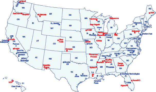
DATA SOURCES: Biofuels Digest (2010) and DOE-EERE (2011).
A number of companies that have DOE funding have proposed cellulosic biofuel facilities or begun construction of pilot-scale4 or commercial-scale5 facilities (Biofuels Digest, 2010). In each case, a combination of factors has motivated site selection, including feedstock supply, infrastructure, and federal, state, or local financial support for development at that location. In many instances, lists of proposed facilities or those under construction or in operation do not conform to those locations predicted by the siting models or analyses discussed. The site-specific nature of biofuel feedstock production, fuel demand and use, and other factors not easily reducible to general model formulations might influence industry decisions. For example, the models estimated that few biorefineries will be sited in the western and northeastern United States, other than the ones that rely on MSW as feedstock. Innovative businesses may recognize feedstock supplies and other advantages overlooked in larger, aggregated analyses.
Comparing Estimated Supplies from Different Studies
The different studies described above all concluded that the United States is capable of producing a sufficient quantity of cellulosic biomass to achieve the RFS2 mandate. The USDA and BDRB reports only estimated potential locations of feedstock supply. NBSM and the EPA Transport Tool also project locations of biorefineries on the basis of where feedstocks could be produced or harvested, feedstock costs, and other factors. In all cases, potential locations of feedstock supplies are based on agroecological classification. (See Chapter 2 for agroecological regions suitable for various biomass types.)
Although the different approaches were independent efforts to assess future feedstock production and related biofuel supplies, they have some commonalities (Table 3-4). All approaches account for the need to leave some residue in the field to prevent soil erosion, but none of them explicitly include water availability as a constraint. Many studies rely on similar data, on the use of a few critical models, or on the work of the same scientists or models. The federal government is the source of much data used by modelers in estimating feedstock supply and future biorefinery locations. For cropland use and other agricultural data nationwide, the USDA-NASS reports result from hundreds of surveys they conduct annually (USDA-NASS, 2011). Those reports cover most aspects of U.S. agriculture, including production and supplies of food and fiber, prices paid and received by farmers, farm labor and wages, farm finances, chemical use, and changes in the demographics of U.S. producers. USDA’s Economic Research Service collects the annual Agricultural Resource Management Survey (ARMS). These data are USDA’s primary source of information on the financial condition, production practices, resource use, and economic well-being of American farm households. ARMS provides observations on field-level and livestock management practices, the economics of farm businesses, and the characteristics of American farm households (for example, age, education, occupation, farm and off-farm work, types of employment, and family living expenses). The National Resources Inventory maintained by NRCS has been used to define farm structure (USDA-NRCS, 2010). These surveys form a series from 1982 and provide updated information on the status, condition, and trends of land cover and land use, land capability classes, soil and soil erosion, water and irrigation,
______________
4 A pilot demonstration for biofuel refinery is a facility that has the capacity to process 1-10 dry tons of feedstock per day.
5 A commercial demonstration for biofuel refinery is a facility that has the capacity to process 700 dry tons of feedstock per day.
| Source | National Biorefinery Siting Model | U.S. Environmental Protection Agency (EPA) | Biomass Research and Development Initiative | University of Tennessee and Oak Ridge National Laboratory (ORNL) | |
| Data or model sources for feedstocks | Crops | USDA-NASS (U.S. Department of Agriculture National Agricultural Statistics Service) | USDA-NASS USD A-ARMS (U.S. Department of Agriculture Agricultural Resource Management Survey) FASOM (Forest and agricultural sector optimization model) | USDA-NASS USDA-ARMS |
USDA-NASS USDA-NRI (U.S. Department of Agriculture National Research Initiative) Data from ORNL |
| Crop residue | USDA-NASS SURGO (Soil survey geographic database) RUSLE (Revised Universal Soil Loss Equation) | USDA-NASS | USDA-NASS SURGO RUSLE |
||
| Dedicated bioenergy crops | PNNL (Pacific Northwest National Laboratory) | PNNL CRP (Conservation Reserve Program) land excluded |
POLYSYS (Policy Analysis System Model) CRP land excluded |
PNNL Jager et al. (2010) |
|
| Forest residue | FIA (Forest Inventory and Analysis National Program) U.S. Department of Agriculture Forest Service (USFS) (2010) |
FIA FASOM |
FIA | FIA USFS (2010) |
|
| Municipal Solid Wastes | EPA Arsova et al. (2008) |
EPA | |||
| Livestock | FASOM | USDA-NASS | |||
| Infrastructure | Bureau of Transportation Statistics | ||||
| Models | Original optimization model RUSLE FRCS (Fuel Reduction Cost Simulator) |
FASOM Siting tool |
REAP (Rural Energy for America Program) POLYSYS EPIC (Environment Policy Integrated Climate Model) |
POLYSYS IMPLAN (Impact analysis for planning) economic modeling FRCS |
|
| Source | National Biorefinery Siting Model | U.S. Environmental Protection Agency (EPA) | Biomass Research and Development Initiative | University of Tennessee and Oak Ridge National Laboratory (ORNL) | |
| Description/scenarios | Minimizes the cost of meeting biofuel targets on a national level, subject to local biomass supplies and infrastructure availability. Diverse price scenarios modeled. |
Minimizes the cost of meeting biofuel targets on a national level, subject to local biomass supplies and local capital costs. | Uses projected crop yields, land availability, and targeted biomass requirements to meet biofuel demand. Diverse yield and demand scenarios modeled. | Uses projected crop yields, land availability, land use transformation, and targeted biomass requirements to meet biofuel demand. Diverse scenarios modeled, including different levels of demand for biomass and fuels, yield levels, and carbon storage payments. |
|
| Environmental restrictions on feedstock production | Erosion and maintenance of soil organic matter | Yes | Yes | Yes | Yes |
| Nutrients Water |
Yes | Yes | Yes | ||
| Greenhouse gas | Yes | Yes | Yes | ||
| Biomass power considered | Yes | ||||
| Biorefinery capital costs | Yes | Yes | |||
| Specific locations of biorefineries | Yes | Yes | |||
| References | Parker (2011) and Parker et al. (2010a) | EPA (2010) | BRDB (2008) | De La Torre Ugarte and Ray (2000), Walsh et al. (2003, 2007), Dicks et al., (2009), English et al. (2010), Jager et al. (2010) | |
and related resources on the nation’s nonfederal lands.6 The USFS data form the basis for many assessments of biomass availability from those sectors (USFS, 2010).
Comparisons of projected biorefinery locations and feedstock supplies identified from different studies indicate that there are similarities among studies (Figures 3-4, 3-5, 3-6, and 3-7)—a large amount of crop residues can be derived from the Corn Belt; herbaceous perennial crops will likely be planted in the Southeast; the Pacific Northwest, North Central, and Northeast regions can supply forest residues; and large quantities of MSW, if included, can be supplied from larger urban areas (primarily near urban areas in the Northeast and western states). Both EPA and BRDB estimated that 10 billion gallons of ethanol-equivalent biofuel would be derived from crop residues or dedicated bioenergy crops and 4 billion gallons of ethanol-equivalent biofuels would be derived from forest resources.
Some differences in the outcome of the feedstock supply and biorefinery siting studies were observed. NBSM projected more perennial grass crop production along the western edge of the Corn Belt in the southeastern and northern prairie regions than EPA, English et al. (2010), or BRDB (2008). Compared to the estimations of biorefinery locations provided by NBSM and the feedstock locations provided by USDA and BRDB, EPA projected fewer facilities located in the Corn Belt region, more in the Southeastern United States, and more in California (presumably associated with MSW conversion). The influence of capital costs associated with biorefinery permitting and construction was estimated and used in EPA’s model but not in other siting models. These costs are estimated by EPA to be lower in the Southeast and Midwest than elsewhere. EPA’s projected biorefinery locations were sited in locations with the lowest capital costs. In EPA’s analysis, minimizing capital costs was more important than maximizing the yield of perennial grasses or the availability of forest residues. Nonetheless, many biorefineries are projected to be built in similar regions to those derived from other modeling efforts.
UNCERTAINTIES ABOUT CELLULOSIC FEEDSTOCK PRODUCTION AND SUPPLY
Although NBSM and other studies estimated that 500-600 million dry tons of biomass could be supplied to biorefineries for fuel production, several factors could alter that supply: competition for biomass, potential for pests and diseases, and yield increase as a result of research. Farmers’ willingness to grow or harvest feedstocks also can affect supply, which is discussed in Chapter 6 in the context of social barriers to achieving RFS2.
Cellulosic bioenergy crops can be grown for markets other than biofuels. For example, bioenergy crops can be used for power generation (electricity or combined heat and power) or as forage or bedding for animals. Most states (36 out of 50) have set standards that require the electricity sector to generate a portion of the electricity from renewable or alternative sources. Although NBSM accounted for biomass allocated for electricity generation, competition for feedstock between the two sectors could drive up the price of feedstock. The technology for producing fiberboard from sawdust and other residues has improved (Ye et al., 2007; Yousefi, 2009), and crop and wood residues can be used for that purpose and further increase the competition for feedstock.
In the case of agricultural residue, it becomes a commodity with value instead of being a residue that incurs an additional cost of its removal when new market opportunities become available. As discussed in Chapter 2, leaving a portion of crop residue can protect
______________
6 Nonfederal lands include privately owned lands, tribal and trust lands, and lands controlled by state and local governments.
land from soil erosion and maintain soil carbon. The crop residues removed can be used for animal bedding (Tarkalson et al., 2009).
The price and supply of bioenergy feedstocks likely to be available to biorefineries depend partly on competition with other uses, in addition to other factors including production, harvesting, and transportation costs. Whether biorefineries can compete for biomass with other sectors will depend on the prices that other sectors are willing to pay for the feedstocks. For example, the likely value of crop residues as bedding to animal producers is the cost of replacing the residues with a substitute.
Competition for feedstock could intensify during periods of weather extremes (for example, drought or flood) if crops are lost to pests and diseases. Fungal diseases that could affect switchgrass have been reported (Gustafson et al., 2003; Crouch et al., 2009). Insect pests could affect the establishment of switchgrass stands; for example, grass seedlings were reported to be susceptible to grasshoppers, crickets, corn flea beetle, and cinch bug (Landis and Werling, 2010). A preliminary study suggested the yellow sugarcane aphid and the corn leaf aphid as potential pests of Miscanthus × giganteus (Crouch et al., 2009). Although severe pest and disease outbreaks have not been observed for herbaceous perennial crops outside the tropics (Karp and Shield, 2008), the pest and disease dynamics could change if cultivation of these crops increases and become more intensive.
Short-rotation woody crops are susceptible to diseases and pests. Rust diseases can affect poplar and willow severely (Royle and Ostry, 1995). In addition to diseases, insect pests such as cottonwood leaf beetle and defoliators, sap feeders, and stem borers can attack poplar and willow (Landis and Werling, 2010).
Cultivar selection, breeding, and genomic approaches can result in bioenergy crops that are resistant to pests and diseases, suitable for their specific agronomic conditions, and have other desirable characteristics as biofuel feedstock (Bouton, 2007; Nelson and Johnsen, 2008). Increase in yield per acre as a result of agronomic and genetic research (Mitchell et al., 2008; Jakob et al., 2009; Wrobel et al., 2009) could alleviate competition for feedstocks among different sectors.
Several studies estimated that the United States has the capability to produce adequate biomass feedstock for production of 16-20 billion gallons of cellulosic biofuels to meet RFS2. Different types of feedstocks predominate in different regions. In the North Central and Northeast regions, forestry residues are most important. In the southeastern United States, forest residues and perennial grasses are most important. In the prairie regions of the United States, crop residues, corn grain, and perennial grasses are predicted to be produced. Some studies constrain the feedstock supply by price with the intent to simulate feedstock supply at a reasonable cost to biorefineries. However, the studies discussed above do not address the gap between the price that farmers are willing to sell their biomass feedstock and the price that biorefineries are willing to pay. The next chapter assesses the economics of feedstock supply in detail. Most studies also constrain the feedstock supply by limiting the amount of crop residues that could be harvested with the intent of minimizing soil erosion. However, soil erosion is only one of many environmental factors that have to be considered in large-scale production of bioenergy feedstock. Chapter 5 discusses various environmental effects to be considered. Knowing feedstock supply and biorefinery locations, local or biorefinery-specific environmental consequences of biofuel production also can be estimated or anticipated. Potential harvestable biomass feedstock is unlikely to be the limiting factor in meeting RFS2. At the same time, limits associated with the diverse economic and environmental effects of
achieving the RFS2 mandate by 2022 could reduce the amount of biomass feedstock projected to be available in the United States for cellulosic biofuels by independent studies.
Arsova, L., R. van Haaren, N. Goldstein, S. Kaufman and N. Themelis. 2008. The state of garbage in America. BioCycle 49(12):22.
Beach, R.H., and B.A. McCarl. 2010. U.S. Agricultural and Forestry Impacts of the Energy Independence and Security Act: FASOM Results and Model Description. Final Report. Research Triangle Park, NC: RTI International.
Biesecker, R.L., and R.D. Fight. 2006. My Fuel Treatment Planner: A User Guide. Portland, OR: U.S. Department of Agriculture - Forest Service.
Biofuels Digest. 2010. Industry Data. Available online at http://biofuelsdigest.com/bdigest/free-industry-data/. Accessed November 12, 2010.
Bouton, J.H. 2007. Molecular breeding of switchgrass for use as a biofuel crop. Current Opinion in Genetics & Development 17(6):553-558.
BRDB (Biomass Research and Development Board). 2008. Increasing Feedstock Production for Biofuels: Economic Drivers, Environmental Implication, and the Role of Research. Washington, DC: U.S. Department of Agriculture.
BRDB (Biomass Research and Development Board). 2010. BR&D: Biomass Research and Development. Available online at http://www.usbiomassboard.gov/. Accessed November 4, 2010.
Carolan, J., S. Joshi, and B. Dale. 2007. Technical and financial feasibility analysis of distributed bioprocessing using regional biomass pre-processing centers. Journal of Agricultural & Food Industrial Organization 5(2):Article 10.
Crouch, J.A., L.A. Beirn, L.M. Cortese, S.A. Bonos, and B.B. Clarke. 2009. Anthracnose disease of switchgrass caused by the novel fungal species Colletotrichum navitas. Mycological Research 113:1411-1421.
De La Torre Ugarte, D.G., and D.E. Ray. 2000. Biomass and bioenergy applications of the POLYSYS modeling framework. Biomass and Bioenergy 18(4):291-308.
Dicks, M.R., J. Campiche, D. De La Torre Ugarte, C. Hellwinckel, H.L. Bryant, and J.W. Richardson. 2009. Land use implications of expanding biofuel demand. Journal of Agricultural and Applied Economics 41(2):435-453.
DOE-EERE (U.S. Department of Energy-Energy Efficiency and Renewable Energy). 2011. Integrated biorefineries. Available online at http://www1.eere.energy.gov/biomass/integrated_biorefineries.html. Accessed May 12, 2011.
Egbendewe-Mondzozo, A., S.M. Swinton, R.C. Izaurralde, D.H. Manowitz, and X. Zhang 2010. Biomass Supply from Alternative Cellulosic Crops and Crop Residues: A Preliminary Spatial Bioeconomic Modeling Approach. Staff Paper No. 2010-07. East Lansing: Michigan State University.
English, B.C., D.G. De La Torre Ugarte, C. Hellwinckel, K.L. Jensen, R.J. Menard, T.O. West, and C.D. Clark. 2010. Implications of Energy and Carbon Policies for the Agriculture and Forestry Sectors. Knoxville: The University of Tennessee.
EPA (U.S. Environmental Protection Agency). 2010. Renewable Fuel Standard Program (RFS2) Regulatory Impact Analysis. Washington, DC: U.S. Environmental Protection Agency.
Gunderson, C.A., E.B. Davis, H.I. Jager, T.O. West, R.D. Perlack, C.C. Brandt, S.D. Wullschleger, L.M. Baskaran, E.G. Wilkerson, and M.E. Downing. 2008. Exploring Potential U.S. Switchgrass Production for Lignocellulosic Ethanol. Oak Ridge, TN: Oak Ridge National Laboratory.
Gustafson, D.M., A. Boe, and Y. Jin. 2003. Genetic variation for Puccinia emaculata infection in switchgrass. Crop Science 43(3):755-759.
Hellwinckel, C.M., T.O. West, D.G.D. Ugarte, and R.D. Perlack. 2010. Evaluating possible cap and trade legislation on cellulosic feedstock availability. Global Change Biology Bioenergy 2(5):278-287.
Hess, J.R., K.L. Kenney, L.P. Ovard, E.M. Searcy, and C.T. Wright. 2009. Commodity-Scale Production of an Infrastructure-Compatible Bulk Solid From Herbaceous Lignocellulosic Bioamss. Volume A: Uniform-Format Bioenergy Feedstock Supply Design System. Idaho Falls: Idaho National Laboratory.
Jager, H., L.M. Baskaran, C.C. Brandt, E.B. Davis, C.A. Gunderson, and S.D. Wullschleger. 2010. Empirical geographic modeling of switchgrass yields in the United States. Global Change Biology Bioenergy 2(5):248-257.
Jakob, K., F.S. Zhou, and A. Paterson. 2009. Genetic improvement of C4 grasses as cellulosic biofuel feedstocks. In Vitro Cellular & Developmental Biology-Plant 45(3):291-305.
Jenkins, B. 2010. National Biorefinery Siting Model: Optimizing Bioenergy Development in the U.S. Presentation. Presentation to the Committee on Economic and Environmental Impacts of Increasing Biofuels Production, March 5.
Johansson, R., M. Peters, and R. House. 2007. Regional Environment and Agriculture Programming Model. Washington, DC: U.S. Department of Agriculture - Economic Research Service.
Karp, A., and I. Shield. 2008. Bioenergy from plants and the sustainable yield challenge. New Phytologist 179(1):15-32.
Khanna, M., X. Chen, H. Huang, and H. Onal. 2011. Supply of cellulosic biofuel feedstocks and regional production patterns. American Journal of Agricultural Economics 93(2):473-480.
Landis, D.A., and B.P. Werling. 2010. Arthropods and biofuel production systems in North America. Insect Science 17(3):220-236.
Larson, J.A., B.C. English, D.G.D. Ugarte, R.J. Menard, C.M. Hellwinckel, and T.O. West. 2010. Economic and environmental impacts of the corn grain ethanol industry on the United States agricultural sector. Journal of Soil and Water Conservation 65(5):267-279.
Malcolm, S.A., M. Aillery, and M. Weinberg. 2009. Ethanol and a Changing Agricultural Landscape. Washington, DC: U.S. Department of Agriculture.
Mitchell, R., K.P. Vogel, and G. Sarath. 2008. Managing and enhancing switchgrass as a bioenergy feedstock. Biofuels Bioproducts & Biorefining-Biofpr 2(6):530-539.
NAS-NAE-NRC (National Academy of Sciences, National Academy of Engineering, National Research Council). 2009. Liquid Transportation Fuels from Coal and Biomass: Technological Status, Costs, and Environmental Impacts. Washington, DC: National Academies Press.
Nelson, C.D., and K.H. Johnsen. 2008. Genomic and physiological approaches to advancing forest tree improvement. Tree Physiology 28(7):1135-1143.
Nelson, R.G. 2002. Resource assessment and removal analysis for corn stover and wheat straw in the eastern and midwestern United States: Rainfall and wind-induced soil erosion methodology. Biomass & Bioenergy 22:349-363.
Nelson, R.G., M. Walsh, J.J. Sheehan, and R. Graham. 2004. Methodology for estimating removable quantities of agricultural residues for bioenergy and bioproduct use. Applied Biochemistry and Biotechnology 113:13-26.
Nelson, R.G., J.C. Ascough II, and M.R. Langemeier. 2006. Environmental and economic analysis of switchgrass production for water quality improvement in northeast Kansas. Journal of Environmental Management 79(4):336-347.
NRC (National Research Council). 2008. Water Implications of Biofuels Production in the United States; Committee on Water Implications of Biofuels Production in the United States. Washington, DC: National Academies Press.
Parker, N., Q. Hart, P. Tittman, M. Murphy, R. Nelson, K. Skog, E. Gray, A. Schmidt, and B. Jenkins. 2010a. Development of a biorefinery optimized biofuel supply curve for the western United States. Biomass & Bioenergy 34(11):1597-1607.
Parker, N., Q. Hart, P. Tittman, M. Murphy, R. Nelson, K. Skog, E. Gray, A. Schmidt, and B. Jenkins. 2010b. National Biorefinery Siting Model: Spatial Analysis and Supply Curve Development. Washington, DC: Western Governors Association.
Parker, N.C. 2011. Modeling Future Biofuel Supply Chains Using Spatially Explicit Infrastructure Optimization. Ph.D. Graduate Group in Transportation Technology and Policy, University of California, Davis.
Perlack, R.D., and B.J. Stokes. 2010. Update of the “billion ton” study. Presentation to the Committee on Economic and Environmental Impacts of Increasing Biofuels Production, May 3.
Perlack, R.D., and B.J. Stokes (Leads). 2011. U.S. Billion-Ton Update: Biomass Supply for a Bioenergy and Bioproducts Industry. Oak Ridge, TN: Oak Ridge National Laboratory.
Perlack, R.D., L.L. Wright, A.F. Turhollow, R.L. Graham, B.J. Stokes, and D.C. Erbach. 2005. Biomass as Feedstock for a Bioenergy and Bioproducts Industry: The Technical Feasibility of a Billion-Ton Annual Supply. Oak Ridge, TN: Oak Ridge National Laboratory.
Renard, K.G., G.R. Foster, G.A. Weesies, D.K. McCool, and D.C. Yoder. 1997. Predicting Soil Erosion by Water: A Guide to Conservation Planning with the Revised Soil Loss Equation (RUSLE). Washington, DC: U.S. Department of Agriculture.
Royle, D.J., and M.E. Ostry. 1995. Disease and pest control in the bioenergy crops poplar and willow. Biomass & Bioenergy 9(1-5):69-79.
Skog, K.E., R.J. Barbour, K.L. Abt, E.M. Bilek, F.Burch, R.D. Fight, R.J. Hugget, P.D. Miles, E.D. Reinhardt, and W.D. Sheppard. 2006. Evaluation of Silvicultural Treatments and Biomass Use for Reducing Fire Hazard in Western States. Madison, WI: U.S. Department of Agriculture - Forest Service.
Skog, K.E., R. Rummer, B. Jenkins, N. Parker, P. Tittmann, Q. Hart, R. Nelson, E. Gray, A. Schmidt, M. Patton-Mallory, and G. Gordon. 2008. A Strategic Assessment of Biofuels Development in the Western States. Proceedings of the Forest Inventory and Analysis (FIA) Symposium.
Tao, L., and A. Aden. 2008. Technoeconomic Modeling to Support the EPA Notice of Proposed Rulemaking (NOPR). Golden, CO: National Renewable Energy Laboratory.
Tarkalson, D.D., B. Brown, H. Kok, and D.L. Bjorneberg. 2009. Irrigated small-grain residue management effects on soil chemical and physical properties and nutrient cycling. Soil Science 174(6):303-311.
Thomson, A.M., R.C. Izarrualde, T.O. West, D.J. Parrish, D.D. Tyler, and J.R. Williams. 2009. Simulating Potential Switchgrass Production in the United States. Richland, WA: Pacific Northwest National Laboratory.
Tittmann, P., N. Parker, Q. Hart, and B. Jenkins. 2010. A spatially explicit techno-economic model of bioenergy and biofuels production in California. Journal of Transport Geography 18(6):715-728.
USDA (U.S. Department of Agriculture). 2010. A USDA Regional Roadmap to Meeting the Biofuels Goals of the Renewable Fuels Standard by 2022. Washington, DC: U.S. Department of Agriculture.
USDA-NASS (U.S. Department of Agriculture - National Agricultural Statistics Service). 2011. Agency overview. Available online at http://www.nass.usda.gov/About_NASS/index.asp Accessed February 3, 2011.
USDA-NRCS (U.S. Department of Agriculture - Natural Resources Conservation Service). 2006. U.S. general soil map (STATSGO2). Available online at http://soils.usda.gov/survey/geography/statsgo/. Accessed November 30, 2010.
USDA-NRCS (U.S. Department of Agriculture - Natural Resources Conservation Service). 2008. Soil Survey Geographic (SSURGO) Database. Available online at http://soils.usda.gov/survey/geography/ssurgo/. Accessed November 30, 2010.
USDA-NRCS (U.S. Department of Agriculture - Natural Resources Conservation Service). 2010. National Resources Inventory. Available online at http://www.nrcs.usda.gov/technical/NRI/. Accessed September 23, 2010.
USFS (U.S. Department of Agriculture - Forest Service). 2010. Forest Inventory and Analysis National Program. Available online at http://fia.fs.fed.us/tools-data/ Accessed November 18, 2010.
Walsh, M., D.G. De La Torre Uguarte, H. Shapouri, and S.P. Slinsky. 2003. Bioenergy crop production in the United States. Environmental and Resource Economics 24(3):313-333.
Walsh, M.E., D.G. De La Torre Ugarte, B.C. English, K. Jensen, C. Hellwinckel, R.J. Menard, and R.G. Nelson. 2007. Agricultural impacts of biofuels production. Journal of Agricultural and Applied Economics 39(2):365-372.
Wrobel, C., B.E. Coulman, and D.L. Smith. 2009. The potential use of reed canarygrass (Phalaris arundinacea L.) as a biofuel crop. Acta Agriculturae Scandinavica Section B-Soil and Plant Science 59(1):1-18.
Ye, X.P., J. Julson, M.L. Kuo, A. Womac, and D. Myers. 2007. Properties of medium density fiberboards made from renewable biomass. Bioresource Technology 98(5):1077-1084.
Yousefi, H. 2009. Canola straw as a bio-waste resource for medium density fiberboard (MDF) manufacture. Waste Management 29(10):2644-2648.
This page intentionally left blank.


