Assessing Highway Tolling and Pricing Options and Impacts: Volume 2: Travel Demand Forecasting Tools (2012)

Below is the uncorrected machine-read text of this chapter, intended to provide our own search engines and external engines with highly rich, chapter-representative searchable text of each book. Because it is UNCORRECTED material, please consider the following text as a useful but insufficient proxy for the authoritative book pages.

73 5.1 Coordination with the SHRP 2 C04 Project The second Strategic Highway Research Program (SHRP 2) includes the closely related large-scale project C04 “Improving Our Understanding of How Highway Congestion and Pricing Affect Travel Demand.” The principal researchers working on the NCHRP Project 08-57 are also leading the SHRP 2 C04 project and are able to closely coordinate these two proj- ects as one coherent body of research. The research agenda of the SHRP 2 C04 project demands both theoretical and applied perspectives; the research objec- tives can be encapsulated as follows: • Theory and research: Develop mathematical descriptions of the full range of behavioral responses to congestion, travel time reliability, and pricing, by highway user types. • Application for modeling: Provide guidance for the incor- poration of these mathematical specifications into various demand-modeling systems in use (and under development), recognizing the complex nature of supply-side feedbacks (via traffic assignment and simulation techniques). The SHRP 2 C04 work plan can be conceptualized as a series of three interconnected levels of behavioral rigor and practical application, along with varying levels of sophisti- cation and associated inputs in each. Since supply-demand interactions are critical for congestion and pricing solutions (including network equilibrium), these offer a second dimen- sion, as reflected in Figure 18. Level 1 – Behavioral Foundations. The first level corre- sponds to behavioral models intended for a deep understand- ing and quantitative exploration of travel behavior. These include many kinds of variables, often explicitly controlled under stated-preference settings (e.g., preferred arrival time and schedule flexibility) and not all of which can be produced by most network/supply-side models (e.g., travel time reli- ability, particularly in the event of non-recurring incidents). These models seek to address the full range of possible short- and long-term responses, but also may focus on selective choice dimensions (for example, route and departure time choices, or home location choice). Supply-side variables for such models can be based on observed and/or generated measures of congestion, reliability, and price (via, for example, an SP survey design). Multiple, repeated observations can be used for the direct derivation of reliability measures. Typically, there is no consideration of equilibrium at this stage, and the linkage between the demand and supply sides is essentially one-directional (as suggested in Figure 18). Research associated with the widest possible range of behav- ioral responses is important for the construction of an “ideal” behavioral model – free of implementation constraints and capable of serving as the starting point for operational models, via some simplifying assumptions. In particular, the explor- atory level of the research will consider dynamics—within- day, as well as day-to-day variations; different time frames for travel adjustments—short-term (which must also account for the with effect of information), medium-term and long- term, as well as the correspondence of the time scale to differ- ent choice dimensions. For example, in certain situations for short-term analysis, route choice might be the only relevant dimension, while departure time choice is equally important in day-to-day, medium- and long-term responses. Level 2 – Advanced Operational. The second level relates to relatively advanced, yet operational, tour-based ABMs, integrated with state-of-the-art DTA models. These mod- els allows for the incorporation of a wide range of possible short-term and long-term responses that are embedded in the choice hierarchy of the model structure. For example, a traveler’s acquisition of an E-ZPass or transponder may be linked to his/her subsequent choice of payment type (at the lower level of the behavioral hierarchy). The integrity C h a p t e r 5 Strategic Directions for Improvement

74 of operational models requires that each and every choice dimension should be allocated a proper “slot” in the hierar- chy, with upward and downward linkages to related choices. Operational/computing time requirements often limit the total number of choice dimensions and alternatives, but this source of restriction is lessening with time. Another relevant constraint in model application is that all measures of con- gestion, reliability, and price be compatible with the demand model’s specification, and can be generated by the network simulation. Moreover, the demand and supply side should be integrated in an equilibrium setting, which imposes cer- tain limitations on how variables like travel time variability are generated, since direct methods based on multiple obser- vations of the same trip typically are generally infeasible in application. Consequently, the issue of generating opera- tional proxies for travel time reliability is one of the focused points of the research. Level 3 – Opportunities for Prevailing Practice. The third level relates to existing model systems used by most of MPOs and state DOTs, mostly in the form of aggregate 4-step trip-based models. Though rather restrictive in design, such models offer opportunities for meaningful and immediate contributions to the state of travel demand modeling prac- tice. While conventional frameworks emphasize short-term responses to congestion and road pricing policies (including changes in route, mode, and, in some cases departure time choices, for each trip segment), road pricing can be addressed in trip distribution and even trip generation components through generalized cost impedances (or mode choice Log- sums) and accessibility measures. The conventional model framework also allows for some indirect reflection of pric- ing on long-term choices, including workplace location and car ownership. A serious restriction of conventional models (also inherited by most current activity-based tour-based models) is that these rely on static assignment procedures. Static assignments generate only crude average travel time and cost variables, and reliability can be implemented only through simplified proxies. The adopted approach for the SHRP 2 C04 research is pred- icated on pushing the boundary of network models in order to achieve greater behavioral sensitivity within the demand models, along with a natural integration of all system compo- nents. While several advanced models and methods presently exist, these require special data sets and longer run times, along with other use restrictions, many of which are purely technical. For example, DTA at a full regional scale is not yet realistic, although with ongoing computational advances and parallel processing opportunities a dramatic break- through may be anticipated within the next 5 to 10 years. The current constraints on practical applications also place limitations on the demand models in terms of possible num- ber of choice dimensions and numerical realizations in the microsimulation process. Figure 18. Levels of sophistication in SHRP 2 project.

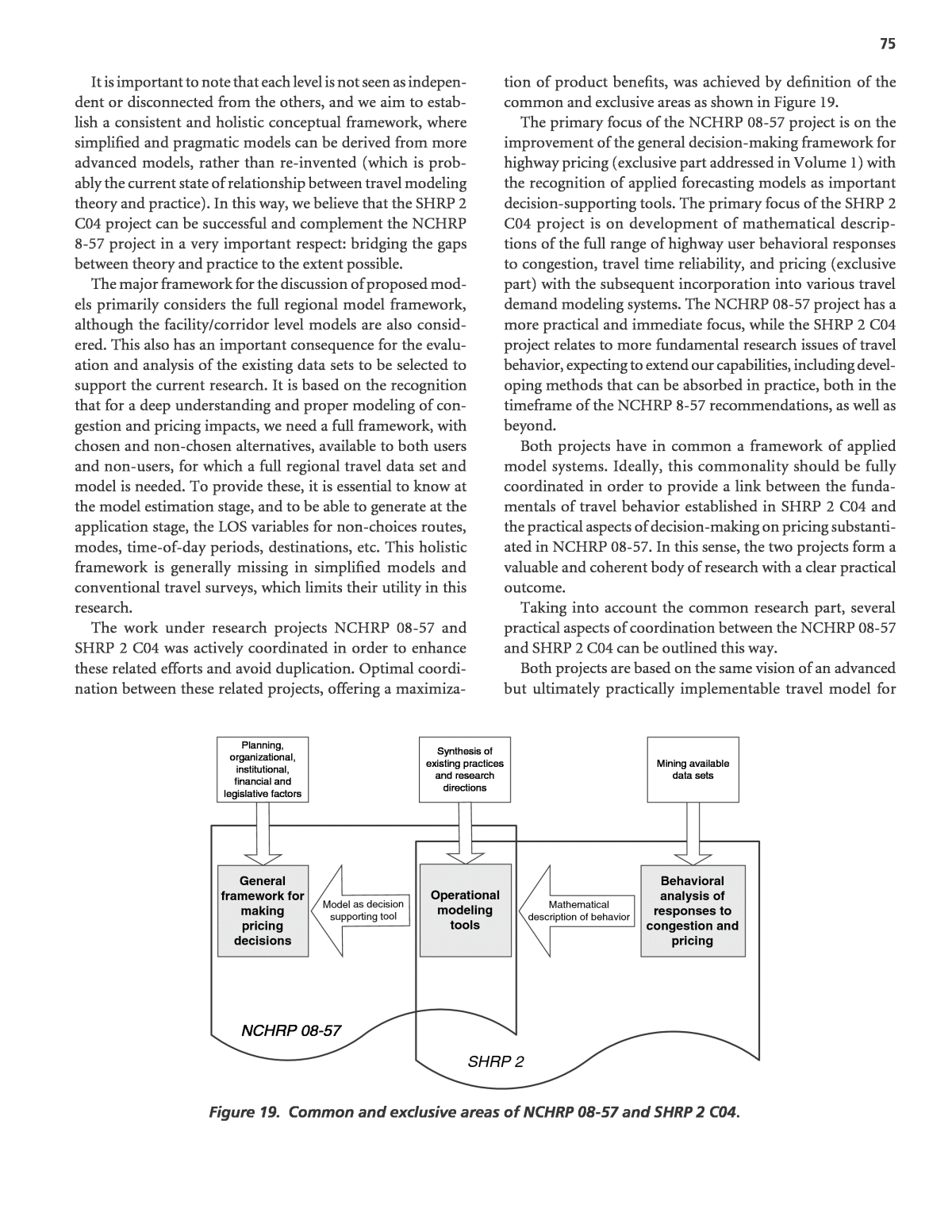
75 It is important to note that each level is not seen as indepen- dent or disconnected from the others, and we aim to estab- lish a consistent and holistic conceptual framework, where simplified and pragmatic models can be derived from more advanced models, rather than re-invented (which is prob- ably the current state of relationship between travel modeling theory and practice). In this way, we believe that the SHRP 2 C04 project can be successful and complement the NCHRP 8-57 project in a very important respect: bridging the gaps between theory and practice to the extent possible. The major framework for the discussion of proposed mod- els primarily considers the full regional model framework, although the facility/corridor level models are also consid- ered. This also has an important consequence for the evalu- ation and analysis of the existing data sets to be selected to support the current research. It is based on the recognition that for a deep understanding and proper modeling of con- gestion and pricing impacts, we need a full framework, with chosen and non-chosen alternatives, available to both users and non-users, for which a full regional travel data set and model is needed. To provide these, it is essential to know at the model estimation stage, and to be able to generate at the application stage, the LOS variables for non-choices routes, modes, time-of-day periods, destinations, etc. This holistic framework is generally missing in simplified models and conventional travel surveys, which limits their utility in this research. The work under research projects NCHRP 08-57 and SHRP 2 C04 was actively coordinated in order to enhance these related efforts and avoid duplication. Optimal coordi- nation between these related projects, offering a maximiza- tion of product benefits, was achieved by definition of the common and exclusive areas as shown in Figure 19. The primary focus of the NCHRP 08-57 project is on the improvement of the general decision-making framework for highway pricing (exclusive part addressed in Volume 1) with the recognition of applied forecasting models as important decision-supporting tools. The primary focus of the SHRP 2 C04 project is on development of mathematical descrip- tions of the full range of highway user behavioral responses to congestion, travel time reliability, and pricing (exclusive part) with the subsequent incorporation into various travel demand modeling systems. The NCHRP 08-57 project has a more practical and immediate focus, while the SHRP 2 C04 project relates to more fundamental research issues of travel behavior, expecting to extend our capabilities, including devel- oping methods that can be absorbed in practice, both in the timeframe of the NCHRP 8-57 recommendations, as well as beyond. Both projects have in common a framework of applied model systems. Ideally, this commonality should be fully coordinated in order to provide a link between the funda- mentals of travel behavior established in SHRP 2 C04 and the practical aspects of decision-making on pricing substanti- ated in NCHRP 08-57. In this sense, the two projects form a valuable and coherent body of research with a clear practical outcome. Taking into account the common research part, several practical aspects of coordination between the NCHRP 08-57 and SHRP 2 C04 can be outlined this way. Both projects are based on the same vision of an advanced but ultimately practically implementable travel model for General framework for making pricing decisions Operational modeling tools Behavioral analysis of responses to congestion and pricing Model as decision supporting tool Mathematical description of behavior NCHRP 08-57 SHRP 2 Planning, organizational, institutional, financial and legislative factors Synthesis of existing practices and research directions Mining available data sets Figure 19. Common and exclusive areas of NCHRP 08-57 and SHRP 2 C04.

76 highway pricing studies. This model should include a well- defined set of features including synthesis of the best practices (corresponds to the short-term improvements described in Chapter 4) and the most important and realistically projected breakthroughs (long-term improvements classified in the sub-section that follows). The conceptual model structure that would serve as the core for both research projects will be outlined in two ver- sions that correspond to two existing conventional modeling approaches: • Aggregate trip-based 4-step models. Although most of the new large-scale regional models developed/being developed after year 2000 have already been activity-based, these models still constitute a majority of the applied models on the market. It should be recognized, however, that while the conventional model structure has many limitations, it does allow for numerous improvements, especially for lower-level choice dimensions (route and mode). Using the SHRP 2 project terminology introduced in Figure 15, only the third level of sophistication can be incorporated in this model structure. • Activity-based tour-based microsimulation models. These models are now rapidly becoming accepted in practice in major metropolitan regions, including regions undergoing comprehensive pricing studies (San Francisco, New York, Denver, Atlanta, Seattle, Los Angeles). This model struc- ture offers numerous additional opportunities that corre- spond to the second level of sophistication. Among them are advantages of individual microsimulation (practically any level of deterministic and/or probabilistic segmenta- tion of users), as well as a better framework for capturing upper-level choices (daily activity patterns and schedules, transponder acquisition, car ownership, etc.). The conceptual model structure can have many specific technical details depending on the pricing project (as dis- cussed in Chapter 4). In practical terms, and taking into account that most of the comprehensive pricing studies con- sider multiple project alternatives, it makes sense to make an effort to prepare a modeling tool that could serve a wide range of pricing studies rather than a single predetermined study. From this point of view, two principal types of studies can be distinguished: • Area/Cordon and other global regional pricing studies where multiple facilities are considered in a certain sub- area. For these studies, mode choice, time-of-day choice, as well as upper-level (trip-frequency related) choices are in the focus. These pricing forms are frequently non-trip- based, defined instead as a daily charge or access fee (for multiple trips), which makes activity-based models espe- cially appealing for these studies, since the principal limita- tions of 4-step model structure have become an obstacle for the analysis. • Intercity and corridor-specific pricing studies where a single facility is considered with possible multiple cross-section design, access, vehicle eligibility, and lane management/pricing form alternatives, including dynamic (state-dependent) pricing. For these studies, the route choice dimension, specifically a binary choice between managed lanes and general-purpose lanes, represents the core issue. Vehicle occupancy and time-of-day choice dimensions are also important if the corresponding pricing forms (HOV/ HOT lanes, congestion pricing) are the focus of the study. Mode choice might be a secondary issue, if a strong transit alternative (or integration of BRT in the managed lane) is considered. Upper-level choices that relate to trip fre- quency are normally less affected. In practical terms, and taking into account that the pricing form itself is a per-trip charge, it makes trip-based models competitive for these projects. Both projects, NCHRP 08-57 and SHRP 2 C04, are in agreement regarding the major breakthrough directions that can form the long-term model improvement program for highway pricing studies. In the following section, these directions are identified and the possible approaches that will be further explored in the framework of the SHRP 2 C04 project area are outlined. 5.2 Breakthrough Directions on the Demand Side The most promising directions for the improvement of road pricing models are shown to be associated with advanced ABMs and advanced network simulation tools (DTA and micro-simulation). Certain significant improvements, how- ever, can also be incorporated within the conventional 4-step modeling framework. More specifically, breakthroughs in the following critical areas are needed to provide for the incorpora- tion of improved model features and components essential for a full and accurate analysis of road pricing projects. • Heterogeneity of road users with respect to their VOT and willingness to pay. This requires a consistent segmenta- tion throughout all of the demand modeling and network simulation procedures to ensure compatibility of implied VOTs. In addition to an explicit segmentation, random coefficient choice models represent a promising tool for capturing heterogeneity. • Proper incorporation of toll road choice in the general hierarchy of travel choices in the modeling system. Addi- tional travel dimensions (such as whether to pay a toll,

77 car occupancy, and payment type/technology), and associ- ated choice models should be properly integrated with the other sub-models in the model system. • Accounting for reliability of travel time associated with toll roads. The incorporation of travel time reliability in applied models requires quantitative measures that could be modeled on both demand and supply sides. • More comprehensive modeling of time-of-day choice based on the analysis of all constraints associated with changing individual daily schedules. • More comprehensive modeling of car occupancy related decisions, including differences in carpool types (planned intra-household, planned inter-household, and casual) and associated VOT impacts. • More advanced traffic simulation procedures such as DTA and microsimulation, and better ways to integrate them with travel demand models. 5.2.1 Approaches to Accounting for Heterogeneity of Highway Users Heterogeneity of road users with respect to their willing- ness to pay for travel time savings (expressed VOT) and higher reliability (value of reliability or VOR) has long been a focus of research and practice of travel modelers. Conceptually, VOT has two components: lost participation in activities, and the undesirability of travel per se. Most logit mode choice models use simple representations and assumptions about VOT, typically a single value. Two pri- mary means of addressing the heterogeneity of travelers’ values of time are: • Use of segmentation, in which the time-of-day, mode choice, and assignment procedures (and potentially other compo- nents) are all fully consistent, and in which a single aver- age VOT is assumed within each segment. This approach is commonly used in practice. • Application of probabilistic distributions of VOT instead of single deterministic values, which similarly demands consistent treatment across the time-of-day, mode choice, and assignment procedures. This approach provides far greater behavioral fidelity, but has rarely been used in travel demand forecasting practice. Explicit segmentation by VOT has been applied in many mode choice and toll road choice models and has also been incorporated in trip distribution and destination choice models through the use of mode choice Logsums as imped- ance measures. It is uncommon, however, to carry this seg- mentation through the trip assignment stage, since this leads to a proliferation of trip tables and an accompanying increase in the amount of time consumed by the assignment process. Additional segmentation also tends to dampen price sen- sitivity, since a typical sigmoid response curve, like the logit model, has the steepest (most elastic) part in the middle, while the ends are quite flat. Stated otherwise, aggregation across different segments tends to yield average utilities in the middle of the curve, and consequently to overestimate price sensitivity. Explicit segmentation can be an effective way to improve the accuracy of the model, while keeping to a simple analytical form. There are, however, drawbacks to the use of segmenta- tion. First, the number of segments may quickly become infeasible if the segmentation is applied across all dimen- sions simultaneously. Secondly, and more importantly, even the most elaborate segmentation cannot include all possible situational variables that create significant additional varia- tion of VOT within each ideally homogeneous segment. For example, a worker may exhibit a different willingness to pay when they have only a short time to get to and participate in an important business meeting than the average willingness to pay of this worker. In addition, another source of VOT variation is that a significant number of workers may have full or partial reimbursement of their travel costs by their employer or client. The limitations on segmentation make the probabilistic approach to VOT more attractive. Recent theoretical advances in random coefficients (or mixed) logit model estimation make it a plausible option for modeling road-pricing choices. The random coefficient logit form directly represents the situation where the values of time and underlying utility coef- ficients for travel time and cost are assumed to be randomly distributed, rather than deterministic. As a result, the need for segmentation is reduced. Random coefficient estimation capabilities are already available in some commercial estima- tion software such as ALOGIT and LIMDEP. However, there are also significant complications asso- ciated with the estimation and implementation of random coefficient logit models. Specification of these models, and analysis of model estimates, requires considerably more effort than is required for traditional closed forms. In addition, the implementation of these models is also different than application of standard logit models and requires additional effort. While the random coefficient models might provide greater behavioral realism, use of this leading edge approach will require significantly more effort and an increase in the commitment of resources. In many regional models, the segmentation used in travel demand choice models, such as time-of-day and mode choice, is frequently inconsistent or even contradictory to the assign- ment procedures used. For example, travel models are nor- mally segmented by purpose while vehicle classes in assignment relate to occupancy only. The need to evaluate road pricing

78 policies presents additional complications and may exacerbate VOT inconsistency issues. The objective behind the optimal segmentation structure is to treat VOT consistently across all choices, while avoiding an excessive proliferation of travel segments and vehicle classes. As noted earlier, additional segmentation of the behavioral choice models in the activity-based framework is less onerous than in conventional 4-step models, but complicating issues associated with the multiplication of vehicle classes in the assignment procedure are shared by both activity-based and conventional models. The choice of the number of vehicle occupancy categories in the assignment procedure should be based on the expected nature of HOV/pricing policies to be modeled. When signifi- cant projects with specific HOV3+ lanes or pricing policies are expected, it generally would require explicit segmentation of trip tables by SOV, HOV2, and HOV3+ classes. Otherwise, collapsing of all HOV categories together can be adopted. Even in the absence of specific traffic restrictions or pricing policies, however, a better segmentation by vehicle occu- pancy can be beneficial to capture differential VOT. In order to avoid a proliferation of segments in the assign- ment step, it may be possible to combine those segments or trip tables with similar VOT. This aggregation should also con- sider additional vehicle classes associated with non-passenger travel such as heavy and light commercial trucks. A final deci- sion about the aggregation of demand or trip tables can only be made after statistical estimation of all VOT and occupancy- related coefficients. It should be understood, however, that any conceivable seg- mentation of VOT by trip purpose, income group, time of day and household/person characteristics will not entirely solve the problem since there is a great deal of situational variability within each segment (and even for the same person during the course of the day). Typical forecasting models, such as logit and probit choice models, assume a normal or bell-shaped distribution around the estimated parameters. If the actual shape of the distribution is not bell-shaped (symmetric), the forecasts are biased, particularly at higher price levels. There are several practical ways to statistically estimate VOT distributions. Probably the simplest approach is based on SP surveys with multiple observations (experiments) for each person and trip. These surveys can be used to obtain individual-level estimates that can be then used to construct the distribution shape. More complex techniques include the estimation of mixed (random coefficients) logit model and latent class models. Both approaches have strengths and weaknesses. They can also be effectively combined. While significant progress has been made in estimation methods and software (that essentially make estimation of a probabilistic VOT available), a bigger challenge is associated with the operational incorporation of VOT distributions in applied travel models. The following possible ways to incor- porate distributed VOT have been identified: • Use the VOT distribution for definition of VOT segments and then employ multi-class assignments and segmented models with average VOT estimated for each segment. • Employ a microsimulation technique that is already embed- ded in ABMs, where each person trip is assigned a specific VOT from the distribution. These (probabilistic) VOT val- ues are saved for each trip and then serve as an important parameter when individual trips are converted into seg- mented trip tables for a conventional static assignment, or even as single agent attributes when linked to a possible DTA or traffic microsimulation method. In the two following sub-sections, we discuss technical details of deterministic travel segmentation that accounts for heterogeneity that is observed, and probabilistic segmenta- tion through continuous distributions of model parameters that accounts for unobserved heterogeneity. 5.2.2 Travel Segmentation (Observed Heterogeneity) This sub-section is based on the recent synthesis and interim findings from the SHRP 2 C04 project. Significant progress has been made in recent years to better understand how motorists value their time while driving. The two key attributes to consider when identifying and segmenting travel markets are VOT and VOR. Another long-term gap in understanding and modeling congestion and pricing is associated with poor segmentation of population and travel. It has generally been recognized by both researchers and practitioners that the profession should move away from crude average VOT estimates (and other related behavioral parameters) obtained from aggregate anal- yses (Hensher and Goodwin 2005). There are a significant number of research works provid- ing insights into behavioral mechanisms and statistical evi- dence on heterogeneity of highway users across different dimensions. Although income and trip purpose have been traditionally used in many models as the main factors that determine VOT, VOT is also a function of many other vari- ables in reality. In fact, in many cases, income and trip pur- pose might not even be the most important factors, especially when situational factors and time pressure come into play Spear (2005), Vovsha, et al. (2005). A variety of traveler and trip type dimensions are impor- tant. The main groups are: • Socio-economic segments of population. These character- istics are exogenous to all activity and travel choices that

79 are modeled in the system. The corresponding dimensions can always be applied for any model either for full segmen- tation or as variables in the utility function. • Segmentation of activities. These characteristics are exog- enous to travel choices but endogenous to activity-related choices. Thus, in the model system, it should be ensured that the corresponding activity choices are modeled prior to the given model; otherwise they cannot be used for model segmentation. • Travel segmentation. These characteristics are endogenous to the system of travel choices. In the mode estimation they have to be carefully related to the model structure to ensure that all dimensions/variables used in each particular model have been modeled prior in the model chain. The socio-economic segmentation of the traveler popula- tion should address the following characteristics: • Income, age, and gender. A higher income is normally associated with higher VOT (Brownstone and Small 2005, Dehghani, et al. 2003), along with middle-age female sta- tus (Mastako 2003, Travel Demand Model Development for T&R Studies in the Montreal Region 2003). • Worker status. Employed persons (even when traveling for non-work purposes) are expected to exhibit a higher VOT compared to non-workers because of the tighter time con- straints (PB Consult 2005). • Household size and composition. Larger households, with children, are more likely to carpool and take advan- tage of managed lanes (Stockton, et al. 2000; Vovsha, et al. 2003). The segmentation of activities may best address the following list: • Travel purpose. Work trips and business-related trips normally are associated with higher VOT as compared to non-work purposes (Dehghani, et al. 2003, NYMTC Transportation Model and Data Initiative 2004, Travel Demand Model Development for T&R Studies in the Mon- treal Region 2003). Airport trips are another frequently cited trip purpose with relatively high VOT (Spear 2005). The list of special trip purposes with high VOT might also include escorting passengers, visiting place of worship, medical appointment, and other fixed-schedule events (theater, sport event, etc). A deeper understanding of the underlying mechanisms for such behavior is valuable, including combinations of schedule inflexibility, low trip frequency, and situational time pressure. • Day of week: weekday versus weekend. There is statistical evidence that VOT for the same travel purpose, income group, and travel party size on weekends is systematically lower than on weekdays, including some examples of posi- tive travel utility associated with long discretionary trips (Stefan, et al. 2007). It is yet to be determined if these differences can be explained by situational variables or if there is an inherent weekend type of behavior different from the regular weekday behavior. In any case, whether directly or as a proxy for situational time pressure, it would be useful to test the differences statistically. The positive utility of travel manifests itself most notably in choice of distant destinations for discretionary activities on week- ends (sometimes with a sightseeing component). This issue should be explored, however, to determine if this is actu- ally correlated with tolerance to congestion delays and unwillingness to pay tolls. • Activity/schedule flexibility. Fixed-schedule activities are normally associated with higher VOT for trips to activ- ity because of the associated penalty of being late; this has manifested itself in many previous research works when VOT for morning commute proved to be higher compared to the evening commute. Probably a similar mechanism (high penalty of being late) creates higher VOT estimates, as it does for trips to airports reported. Schedule flexibility will also be an important factor for non-work activities; a trip to a theater might exhibit a high VOT while shopping might be more flexible. • Situational context: time pressure versus flexible time. This is recognized as probably the single most important factor determining VOT that has yet proven difficult to measure and estimate explicitly, as well as to include in applied models (Spear 2005, Vovsha, et al. 2005). There is evidence that even a low-income person would prob- ably be willing to pay a lot for travel time savings if he/she is in danger of being late to a job interview or is escorting a sick child. This factor is correlated with the degree of flexibility in the activity schedule (inflexible activities, trips to airport, fixed schedules, and appointments will be the activities most associated with time pressure), but does not duplicate it. It might be expected that even for a high income person traveling to the airport, the VOT might not be that high if this person has a 4-hour buffer before the departure time. With ABMs we could use the number of trips/activities implemented by the person in the course of a day, as well as the associated time window available for each trip/activity as an instrumental proxy for time pressure. The segmentation of travel characteristics may best address the following list: • Trip frequency. More regular trips, and their associated costs, may receive more (or less) formal consideration than

80 those that occur infrequently. For example, a $1.50 for auto trip to work may be perceived as $3.00 per day (assuming a symmetric toll) and $60 per month, thus receiving special consideration. This perceptional mechanism is likely very different for infrequent and irregular trips where the toll is perceived as a one-time payment. For intercity trips, trav- elers’ recognition of the return trip is not obvious, since it may occur on a different day. • Time-of-day. Prior research confirms that AM and PM peak periods are generally associated with a higher VOT, as compared to off-peak periods. In particular, it seems this may be the result of more commute trips in these periods and/or higher congestion levels. In addition to that, AM travelers (mostly commuters) are more sensitive to travel time and reliability than PM commuters (who mostly are returning home) (Brownstone, et al. 2003). However, few have explored how these phenomena relate to schedule flexibility, or how time-of-day factors impact VOT for non- work trips. One may reasonably speculate that a model that explicitly accounts for reliability and schedule constraints would not need an additional differentiation by time-of- day periods. • Vehicle occupancy and travel party composition. While a higher occupancy normally is associated with higher VOT (though not necessarily in proportion to party size), it is less clear how travel party composition (for example, a mother traveling with children, rather than household heads traveling together) affects a party’s VOT. • Trip length or distance. Interesting concave functions have been estimated for commuters’ VOT (Steimetz and Brownstone 2005). For short distances, VOT is compara- tively low, since travel time is insignificant and delays are tolerable; for trip distances around 30 miles, VOT reaches a maximum. However, for longer commutes, VOT decreases again since they presumably have chosen residential and work places fully understanding that long- distance commuting will be necessary. Additionally, in the context of mode choice, strong distance-related posi- tive biases have been found for rail modes in the presence of congestion [as a manifestation of reliability (NYMTC 2004)] and carpools (since carpools are associated with extra formation time). • Toll payment method. This is an important additional dimension that has not yet been fully explored. Changes in toll policies implemented by the Port Authority of New York and New Jersey convincingly showed that the introduction of E-Z Pass attracted a significant new wave of users despite a relatively small discount (Evaluation Study of PANYNJ Time of Day Pricing Initiative 2005). In the same way researchers regard perceived time versus actual time differently, they should also probably consider perceived value of money in the context of pricing. Bulk discounts and other non-direct pricing forms should be modeled at the daily pattern level rather than trip level. It is also important to understand congestion impacts on entire daily patterns, rather than by single trips, including an analysis of daily time budgets and trade-offs made to overcome congestion (including work from home, com- pressed workweeks, compressed shopping, moving activi- ties to weekends, etc.). • Congestion level that has an impact on travelers’ percep- tion of time. There is a growing body of evidence that VOT (and willingness to pay) depends on the level of congestion (Wardman, et al. 2009, NCHRP Report 431 1999). In par- ticular, a mark-up value of 2.0–2.5 was reported when VOT in highly congested conditions was compared to free-flow conditions. The concept of perceived highway time differ- entiated by congestion levels is discussed in Section 5.2.4 as one of the practical ways to account for the effects of reli- ability on demand. Congestion levels are correlated with time-of-day periods though there are certain specifics of AM and PM periods beyond just the level of congestion. For example, most of the commute trips in AM period are outbound trips to work that are characterized by a con- strained schedule. Most of the trips in PM period (as well as in off-peak period) are more flexible in terms of departure and arrival time. In model formulation, estimation, and application, it is cru- cial to follow a conceptual model system design and to obey consistent rules of application of those variables that are exoge- nous to the current model. For example, if TOD model is placed after mode and occupancy choice, the mode and occupancy can be used as the TOD model segmentation. However, time of day in this case cannot be used for segmentation of the mode and occupancy choice models. If the order of models is reversed (TOD choice before mode & occupancy choice) the segmenta- tion restrictions would also be reversed. When different models are estimated, it is essential to keep a conceptual model system (or at least a holistic framework) in mind to make these models compatible and avoid endogeneity-exogeneity conflicts. It should be understood that these dimensions cannot be simultaneously included in operational models, as explicit segments in a Cartesian combination. With a 4-step model framework, this would immediately result in an unfeasibly large number of trip tables. The ABM framework is more flexible, and, theoretically, can accommodate any number of segments. They are, however, still rather limited in practical terms by the survey sample size (normally several thousands of individuals) that quickly wears thin for multidimensional segments. There are, however, other ways to constructively address segmentation in operational models that we can con- sider. These include flexible choice structures with parameter- ized probabilistic distribution for parameters of interest (for

81 example, VOT), as well as aggregation of segments by VOT for assignment and other model components that are espe- cially sensitive to dimensionality. It should also be understood that VOT represents only one possible behavioral parameter, and that it is essentially a derived one. In most model specifications and correspond- ing estimation schemes, VOT is not directly estimated, but rather derived either as the ratio of the time coefficient to cost coefficient (in simple linear models as specified in Sec- tion 2.2 as the marginal rate of substitution between time and cost (in a general case). Thus, very different behaviors can be associated with the same VOT. For example, both time and cost coefficients can be doubled which leaves the VOT unchanged; however, this would be a manifestation of very different estimated responses to congestion and pricing. Large coefficients will make the model more sensitive to any network improvement or change in costs, while smaller coef- ficients will make it less sensitive. One of the most detailed VOT segmentation analyses of the type described in the previous sub-section was carried out for the Netherlands National Value of Time study (Bradley and Gunn 1991), which used 10 simultaneous segmentation variables. A similar approach was used for national studies in the United Kingdom and Sweden. All else being equal, a more detailed segmentation typi- cally tends to dampen the overall price sensitivity across the population, since a typical sigmoid response curve, like the logit model, has the steepest (most elastic) part in the middle, while the ends are quite flat, and market segmentation tends to move distinct groups away from the middle. Travel market segmentation is principally different with AB models implemented in a microsimulation fashion compared to aggregate 4-step models. Practically speak- ing, AB models using microsimulation methods do not have limits in terms of segmentation. They can incorpo- rate all of the dimensions listed, and the only constraint that should be taken into account is the ability to estimate VOT (i.e., time and cost coefficients) for each segment with the available data. Essentially, the model estimation results will dictate the segmentation in the model application. A population synthesis procedure embedded in an ABM provides a list of household and persons with all variables available in PUMS, ACS, or other source that are used as a seed micro-sample. Travel segmentation with a 4-step model is constrained in the model application by the set of household and person variables available in the population distribution and sub- sequently by the number of trip tables that would be fea- sible in the trip distribution and mode choice models. This constraint, though technical in nature, severely limits the segmentation that actually can be applied in a 4-step model- ing process. For example, let’s consider a maximum feasible number of segments as 100. This limit will be quickly reached with the following Cartesian combination: • 4 trip purposes (home-based work, home-based school, home-based other, non-home-based), • 3 income groups (low, medium, high). • 4 car ownership groups (zero car, cars fewer than workers, cars equal to workers, cars greater than workers), and • 2 time-of-day periods (peak, off-peak). There is practically no way to include such variables as age, gender, or person status in a 4-step model on top of the basic variables listed above. It is also theoretically impossible to incorporate situational variables or variables that relate to schedule constraints. There are several limited reserves where the segmentation of a 4-step model can be improved. One of them represents a compromise between the segmentation applied in trip distribution versus segmentation applied in mode choice. Trip distribution could be applied with a lim- ited number of segments (say, 96 segments resulted from the variables listed above, or even less). Then, for the mode choice stage, additional segmentation could be applied on the popu- lation side (relevant for home-based trips only) that could include gender, person type, or any other variable. The addi- tional segmentation relates only to the trip origin zones and does not require a separate trip distribution for each segment. In mode choice application, it is assumed that the origin zone proportions for the additional segments are uniform across all destinations. Thus, each trip-distribution segment can be quickly split into sub-segments before mode choice. Another option is to specifically single out travel segments that are characterized by a very high willingness to pay (trips to airports, business trips during the day, etc.) and model them separately with identification of the strongest trip gen- erators on an individual basis. 5.2.3 Probabilistic Distribution of VOT and VOR (Unobserved Heterogeneity) Explicit segmentation can be an effective way to improve the model while keeping it in a simple analytical form. How- ever, there are several strong arguments in favor of probabi- listic treatment of VOT instead of or in addition to explicit segmentation. First, the number of segments quickly becomes infeasible if segmentation is applied across all dimensions simultane- ously. This is especially apparent with conventional, 4-step modeling techniques, which require replication of full OD tables for each combination of segmentation variables (or at least for each distinct value of VOT) for static network traffic assignment. Such detailed travel market segmentation can be much more effectively incorporated in the ABM framework,

82 where each simulated individual and trip can effectively be modeled as having its own levels of VOT (and VOR). The same may be the case for the newest generation of DTA and traffic microsimulation models. Secondly, even if maximum possible segmentation is implemented, a travel model cannot include all possible situ- ational variables that create significant additional variation of VOT within each (seemingly homogeneous) segment. For example, when driving for an important business meeting with very little time available to reach his or her destination, a worker can exhibit a higher willingness to pay than the aver- age for the same person. The same can be said about a mother driving home to attend to a sick child. Also, a not insignifi- cant (but generally unknown) percentage of commuters may have a full or partial reimbursement of their travel cost by the employer. These sources of additional variation are poorly captured in travel surveys, if at all. This means that the proba- bilistic approach of explicitly estimating VOT distributions is bound to be more realistic and more accurate. For example, a recent SP study of users of the new MnPASS HOT lane facility (Zmud, et al. 2007), used a survey method to explicitly estimate each respondent’s individual VOT, and found much more variation across the sample than could be captured through observable segmentation variables alone. The observed distribution resembled the log-normal distri- bution Ben-Akiva, et al. (1993) pioneered an econometric approach to directly estimate the parameters of such log- normal VOT distributions from typical SP and RP data sets. This research was done as part of a study for Cofiroute of proposed tolls on the French national motorways, and the resulting distributed models were applied using a customized multi-user-class static assignment routine. Now, 15 years later, there are a variety of approaches and software available for estimating and applying such models. Random Coefficients (mixed) logit model estimation (already available in commercial software like ALOGIT or LIMDEP or BIOGEME) has become a practical tool for modeling choices related to road pricing. The random coef- ficient logit form directly corresponds to the situation where VOT and underlying utility coefficients for travel time and cost are assumed to be randomly distributed, rather than deterministic (taking single mean values). Since mixed logit requires (computationally intensive) numeric integration for calculation of the choice probabili- ties, this is a certain problem for applying it in an aggregate 4-step model that predicts and accumulates fractional prob- abilities. This problem can be overcome by effective numeric integration. For ABMs based on microsimulation, the situa- tion is even simpler, since there is no need to calculate choice probabilities. Random utilities can be directly simulated from their distributions and then the alternative with the maximum utility would be chosen. This technique eliminates the disadvantages of non-closed form choice models (like probit or mixed logit) and makes them just as convenient as standard logit models in application. In the current research, special attention will be given to the incorporation of mixed logit models (with distributed VOT and VOR) in both micro- simulation and aggregate model frameworks. Note that mixed logit models can also incorporate systematic market segmen- tation, using interaction terms to parameterize (or segment) the distribution according to observed variables. Small, et al. (2005) provide an interesting example of the estimation of a binary model of choice between a toll and a non-toll route that accounts for the heterogeneity of travel- ers with respect to VOT (as well as VOR). In this formula- tion, the non-toll route served as the reference alternative with zero utility while the toll route utility included a con- stant term, various transformations of cost and time differ- ences between the routes, as well as a measure of travel time unreliability. The constant term was specified as a random parameter dependent on such variables as gender, age, and household size. The cost and time coefficients were specified as random parameters interacting with income and trip dis- tance. In this way, the model was able to capture a significant observed heterogeneity (through variables that differentiate the distribution of constant term and time/cost coefficients), as well as residual unobserved heterogeneity through the specification of the random component of the constant, and time/cost coefficients. The utility structure of the model of this type can be written in the following general way: U xsn sn snk nk nk= + + ∑α β ε ( )Equation 18 where s = segments by income, travel purpose, person type, etc, n = observations (instances of choice), k = independent variables like travel time and cost, xnk = values of the independent variables for each obser- vation, as = constant that is assumed to be a random, bsk = coefficients for time and cost that are assumed to be random, and en = random disturbance term. The random constants are specified in the following way: α α ϕ ξsn sl nl n l y= + +∑ ( )Equation 19 where l = variables for capturing observed heterogeneity (like gender and age), ynl = values of the variables for each observation, –a = fixed component (generic alternative-specific bias),

83 jsl = coefficients capturing observed heterogeneity, and xn = random term capturing unobserved heterogeneity. The random coefficients are specified in the following way: β β γ ζskn k skm nm n m z= + +∑ (Equation 20) where m = variables capturing observed heterogeneity (like income and distance), znm = values of the variables for each observation, –bk = fixed components (generic coefficients), gskm = coefficients capturing observed heterogeneity, zn = random term capturing unobserved heterogeneity. The model was estimated based on the combined RP and SP data sets for the California State Route 91. The authors reported significant observed and unobserved heterogeneity among travelers that affects the forecast; a proper accounting for this heterogeneity could enhance the political viability of pricing. In modeling terms, this means that a combination of an explicit segmentation (to account for the observed hetero- geneity) with probabilistic VOT distribution (to account for unobserved heterogeneity) is essential. Randomly distributed VOT has been already incorporated in the new version of practical ABM developed for San Fran- cisco (Figure 20); see Section 6.1. Various ways and levels of highway user segmentation can be considered. The central question is to find a right balance between the explicit (observed) heterogeneity (full or par- tial segmentation of the model coefficients) and unobserved heterogeneity (making some of these coefficients random). For random parameters, different distribution shapes (for example symmetric versus skewed-to-the-left/right VOT dis- tributions) can be explored. From the technical standpoint, randomized VOT is com- paratively simple to apply and it does not affect the model run time. This option, however, is only available with an ABM since it requires an individual microsimulation framework. 5.2.4 Additional Travel Dimensions and Choice Models In order to more faithfully capture the effects of road pricing options, it will be necessary to address additional travel dimensions, such as the choice of whether to pay a toll charge, or the choice of payment type. These choices reflect the willingness of travelers to make tradeoffs between mon- etary costs and travel time savings. Current modeling prac- tice and research provide examples of how these two travel dimensions have been incorporated: • Binary route type choice (toll versus non-toll) can be incor- porated at the lower level in the mode choice hierarchy, as has been implemented in the Montreal model. Introduc- tion of pre-route choice in the mode choice model, and cor- responding enhancements to the subsequent assignment procedures, allows for better accounting of the LOS on toll roads and associated drivers’ perception through toll-road bias, reliability, and other components in the utility function. •Each traveler samples from a V.O.T. distribution, based on their income (Inverse of the lognormal cumulative density function) ($1-$30) •The non-work V.O.T. is set to 2/3 of the work V.O.T. •The same V.O.T. is used for all choice models Figure 20. Randomized VOT applied in San Francisco model.

84 • Car occupancy choice (carpool formation mechanism) can be incorporated either as part of mode choice at the intermediate level (in the auto nest and before pre-route choice) or as an activity-type decision at the tour/trip gen- eration stage. There are also several important differences in formation intra-household and inter-household car- pools that should be taken into account through different modeling techniques. • Payment type/vehicle equipment choice depending on the pricing form and technology can be incorporated in the model system as a lower level in mode choice or time-of- day choice. Representation of a payment type/technology may be essential if several toll-collection technologies with different roadway LOS effects are planned to co-exist for the same facilities. The estimation of models considering the route type and payment type choice dimensions requires a specific and aug- mented set of data. Ideally, the binary pre-route choice model is estimated as part of the mode choice model though an inde- pendent or sequential estimation (first, pre-route choice and then mode choice carrying pre-route choice log-sums up). Intra-household and inter-household carpools are gener- ally modeled in different ways. Intra-household carpools with respect to fully joint tours for non-mandatory activities can be modeled explicitly from the tour generation stage. For these tours the travel party size is predetermined by the household composition and joint-tour participation model with the sub- sequent direct implication for mode choice. For example, if a tour is generated with three participants, SOV and HOV2 modes are automatically made unavailable for this tour (there still can be a choice between HOV3, transit, non-motorized, and taxi modes). For other tours that are either individual or joint (but not modeled explicitly), intra-household carpools are accounted implicitly at the mode choice stage through household size, composition and Daily Activity Pattern vari- ables. For example, for work tours, SOV, HOV2, and HOV3 can be available but such variables as number of workers and school children (or work and school tours) would work in favor of HOV2/HOV3 indicating intra-household carpools and escorting arrangements. Intra-household carpools are gener- ally not extremely sensitive to the HOV LOS characteristics. Inter-household carpools can generally be modeled only implicitly through mode choice. The probability of inter- household carpools to occur does not relate to the household composition, but rather to opportunities to find permanent partners (frequently other workers) with a similar schedule and OD location on the way. Inter-household carpools are more frequent for longer distances, commuters with perma- nent schedules, and commuting to employment centers like CBD. These carpools are typically more sensitive to the HOV LOS characteristics since exclusive HOV lanes or HOT lanes with better levels-of-service than mixed flow lanes may make travelers seek joint travel arrangements. In a mode choice framework, these variables are tested statistically in the HOV mode utility functions. Choice of payment type (including acquisition of tran- sponder) has been recognized as an important dimension for travel segmentation that is currently missing in almost all travel models including the most advanced activity-based models. However, the recent RP surveys of toll users on the existing facilities have clearly shown that travel patterns (and the underlying willingness to pay) of cash users are very dif- ferent from transponder holders (Yan and Small 2000). In particular, transponder holders are characterized by a higher trip frequency, different trip purpose mix, high percentage of symmetric commuters (using the same toll facility for both trip directions), and higher car occupancy. The introduc- tion of a transponder acquisition model (that is essentially a mid-term travel decision relating to a set of mobility choices) would allow for an effective segmentation of highway users, and consequently yield better results for both choice mod- els and traffic assignments. This is essential for T&R forecast studies of highway facilities where manual and ETC toll col- lection technologies coexist. 5.2.5 Incorporation of Travel Time Reliability Quantification of Travel Time Reliability There is a growing body of research and statistical evi- dence, as well as model estimation results, indicating that travelers’ perception of toll roads and willingness to pay is not a simple consideration of average time and cost com- pared to the individual VOT. Willingness to pay for toll roads is also influenced by many other attributes, such as the reli- ability or predictability of travel times through management of roadway capacity, or improved safety through vehicle class restrictions such as trucks. In particular, travel time reliability associated with toll roads has been recognized as a particularly strong factor, and may be as important as, or in certain contexts more important than, average time savings in determining traveler choice. Willingness to pay for reductions in the day-to-day variability of travel time is referred to as VOR. One of the most important strategic directions for improvement of travel models today is the measurement of highway time reli- ability and its impact on travel choices. Several published and ongoing research projects like NCHRP Project 8-64, NCHRP Report 618, SHRP 2 C04, SHRP 2 L04, as well as FHWA guidance are devoted to reliability issues. There has been a considerable body of research regarding the fundamental issues that reflect definition of travel time

85 reliability, its measurement, as well as the computation and treatment of travel time reliability in modeling tools. The suggested reliability measures have been put in the context of effectiveness related to transportation projects, policies, as well as the entire highway system performance. In general, there are four possible methodological approaches to quantify reliability suggested in either research literature or already applied in operational models: • (Indirect measure) Perceived highway time by congestion levels. This concept is based on statistical evidence that in congestion conditions, travelers perceived each minute with a certain weight (NCHRP Report 431 1999, Axhausen, et al. 2006, Levinson, et al. 2004, MRC and PB 2008). Per- ceived highway time is not a direct measure of reliability since only the average travel time is considered though it is segmented by congestion levels. It can, however, serve as a good instrumental proxy for reliability since the perceived weight of each minute spent in congestion is a consequence of associated unreliability. Additionally, it can be mentioned that VOT for different congestion levels does not only include proxies for reliability, but also psychological effects that congestion is more onerous than free-flow travel. For example, a traveler may full well know that he/she will have to sit in highly congested conditions, but perceives the time differently than time spent in free-flow conditions. • (First direct measure) Time variability (distribution). This is considered the most practical direct approach that has received considerable attention in recent years. This approach assumes that several independent measurements of travel time are known, which allow for travel time dis- tribution formation and calculation of some derived mea- sures like buffer time (Small, et al. 2005, Brownstone and Small 2005, Bogers, et al. 2008). One important technical detail with respect to generation of travel time distributions is that even if the link-level time variations are known, it is a non-trivial task to synthesize the OD-level time distri- bution (reliability “skims”) because of the dependence of travel times across adjacent links due to mutual traffic flow. • (Second direct measure) Schedule delay cost. This approach has been adopted in many research works on individual behavior in academia (Small 1982, NCHRP Report 431 1999). According to this concept, direct impact of travel time unreliability is measured through cost functions (pen- alties expressed in monetary terms) of being late (or early) compared to the planned schedule of the activity. This approach assumes that the desired schedule is known for each person and activity in the course of the modeled period. This assumption, however, is difficult to meet in practical model setting. • (Third direct measure) Loss of activity participation util- ity. This method can be thought of as a generalization of the schedule delay concept. It is assumed that each activ- ity has a certain temporal utility profile and individuals plan their schedules to achieve maximum total utility over the modeled period (for example, day) taking into account expected (average) travel times. Then, any deviation from the expected travel time due to unreliability can be associ- ated with a loss of participation in the corresponding activ- ity (or gain if travel time proved to be shorter) (Supernak 1992, Kitamura and Supernak 1997, Tseng and Verhoef 2008). Recently this approach was adopted in several research works on DTA formulation integrated with activ- ity scheduling analysis (Kim, at al. 2006, Lam and Yin 2001). Similar to the schedule delay concept, however, this approach suffers from the data requirements that are dif- ficult to meet in practice. The added complexity of esti- mation and calibration of all temporal utility profiles for all possible activities and person types is significant. This makes it unrealistic to adopt this approach as the main concept for current research, however, it should be con- sidered in future research efforts. Detailed analysis of all four approaches with application examples can be found in Appendix A, Section A.3. A good example of the time variability measure was presented in Small, et al. (2005). The adopted quantitative measure of variability was the upper tail of the distribution of travel times, such as the difference between the 80th and 50th percentile travel times; see Figure 21. The authors argue that this measure is better than a symmetric standard deviation, since, in most situations, being late is more crucial than being early, and many regular travelers will tend to build a “safety margin” into their depar- ture times that will leave them an acceptably small chance of arriving late (i.e., planning for the 80th percentile travel time would mean arriving late for only 20% of the trips). The choice context included binary route choice between the Managed (tolled) Lanes and General Purpose (free) lanes on the section of SR-91 in Orange County, CA. The survey included actual users of the facility and the model was esti- mated on the mix of RP and SP data. The variation of travel times and tolls was significantly enriched by combining RP data from actual choices with SP data from hypothetical sit- uations that were aligned with the pricing experiment. The distribution of travel times was calculated based on the inde- pendently observed data. The measures were obtained from field measurements on SR-91 taken at many times of day, on 11 different days. It was assumed that this distribution was known to the travelers based on their past experience. Reli- ability, as defined above, proved to be valued by travelers as highly as the median travel time. Numerous variations of this approach based on travel time distribution have been proposed. For example, a 95% buffer time threshold was suggested in (CSI 2005) and some

86 additional measures of distribution asymmetry and skew were explored in Bogers, et al. (2008). In the ongoing SHRP 2 Project C04, different variability measures are currently being investigated with respect to their impact on travel demand. Incorporation of Travel Time Reliability in Operational Models One principal problem that hampers making this approach operational is that it requires the explicit modeling of travel time distributions, as well as making assumptions on how travelers acquire information about the random variability they experience. DTA and micro-simulation tools are crucial for the direct assessment of travel time variability, since static assignment can only predict average travel times. However, application and calibration of these dynamic microsimula- tion traffic assignment procedures at the regional level has not often been performed. This principal issue needs both theoretical development and more practical experimenta- tion with the available tools and approaches, even if they are currently operational in small networks only. This issue is in the focus of another SHRP 2 project L04, “Incorporating Reliability Performance Measures in Operations and Plan- ning Modeling Tools,” as well as several research projects currently underway in Europe (ITS 2008). There are, however, several possible practical steps for inclusion of instrumental proxies for reliability measures in operational travel models. They include the recent experi- ence with estimation of VOT by congestion levels (NCHRP Report 431 1999, Wardman 2009) and such measures as amount of congestion delay versus free-flow time applied in the Ottawa travel model (Ottawa TRANS 2007) as well as volume-over-capacity ratios as applied in the Seattle travel model (Appendix A, A.1.1.10). A summary of possible instrumental proxies for indirect measurement of travel time reliability available with a con- ventional static assignment technique is shown in Table 16. These simplified measures could be included in both 4-step models and ABMs. A more detailed discussion on the simplified operational approaches of this type can be found in Appendix A, Section A.3.2 in the context of perceived highway time. 5.2.6 Modeling Time-of-Day Choice and Peak Spreading Time-of-day choice has always been the weakest part of travel models, but this model is essential for forecasting con- gestion pricing schemes. There has been significant progress in modeling techniques for time-of-day choice achieved recently and documented in several research synthesis efforts, as well as incorporated in the first advanced models applied in practice. The following discussion identifies the important features of the new time-of-day choice models and provides 0 0.1 0.2 0.3 0.4 0.5 0.6 0.7 0.8 0.9 1 25 30 35 40 45 50 55 60 Travel time, min Cu m ul at iv e pr ob ab ili ty Difference between the 80th and 50th percentile Figure 21. Travel time variability measure. Core measure Link attribute scaling factors* OD-skim contraction Volume over Capacity (V/C) ratio Number of lanes Average weighted by distance (mean or 50th, 60th, 70th, 80th percentile) Highway facility type Network location (bottleneck) Delay compared to free-flow condition Number of lanes Sum weighted by length Highway facility type Network location (bottleneck) Travel time differentiated by congestion levels Number of lanes Sum weighted by length Highway facility type Network location (bottleneck) * Accounts for probability and impact of accidents and traffic instability Table 16. Instrumental proxies for travel time reliability.

87 recommendations on their estimation and incorporation within the structure of the modeling system: • The new generation of time-of-day models is character- ized by a high level of temporal resolution. These models can predict trip distribution by 30–60 min intervals (or even less if necessary). This is a major breakthrough com- pared to the conventional technique associated with broad (3 hours or longer) time-of-day periods. This advance in practice proved to be possible by hybridizing discrete choice modeling and duration modeling techniques. The results of the time-of-day choice model can be aggregated by broad time-of-day periods in order to provide compat- ibility with conventional period-specific static assignments. They can be more effectively used, however, in combina- tion with DTA/microsimulation tools since these tools rely on demand (trip tables) stratified by fine time slices that can be effectively provided by the new time-of-day models. Even within the conventional static assignment framework, it can be beneficial to distinguish between the sharpest peak hour and shoulders within each peak period (AM and PM) to better portray impacts of congestion pricing. • Modeling theory indicates that the best placement of time- of-day choice model is between destination choice (trip distribution) and mode choice. This means that time-of- day choice should operate with mode choice Logsums as explanatory variables, and mode choice should operate with period-specific travel times and cost. This approach is essential if both mode shifts and peak spreading effects are significant. For corridors and areas where substantial mode choice shifts are not expected, time-of-day choice model can be placed after mode choice (and normally applied for highway trips only). This means that the time- of-day choice model would operate with highway travel times and tolls as variables. In both cases, it is absolutely essential to apply equilibrium feedbacks to ensure that the peak spreading effects are consistent with congested travel time and cost estimates. The new generation of time-of-day choice models can be applied in both 4-step and ABM frameworks. While there are many important similarities in model structure, there are also some principal differences that should be understood: • Time-of-day choice in the 4-step trip-based model frame- work is applied for each trip segment separately. It is lim- ited to the trip table segmentation embedded in the trip generation and distribution structure (by trip purpose, income group, car ownership, etc.). In particular, it is applied for each commuting direction (outbound and inbound from home) separately. As a result, AM peak spreading effects is modeled independently of PM spread- ing effects, and with no explicit control or consistency with the resulting implications for work duration. • Time-of-day choice in the activity-based tour-based model framework is applied for each tour and preserves a consis- tency across all sequential trips in the tour and associated activities. It can also incorporate such important addi- tional variables as person work status (full-time workers versus part-time workers) and household composition (presence of children, etc.). It is applied for the entire com- muting tour (or round trip) in a process that ensures a logical linkage between changing AM and PM departure time. It allows for the explicit control of the duration of work or other activities. A detailed description of the advanced time-of-day choice models with enhanced temporal resolution is included in Appendix A, Section A.4. 5.2.7 Modeling Car Occupancy Several additional factors come into play if pricing or traf- fic restrictions are differentiated by car occupancy. Differ- ent forms of HOV/HOT lanes have been recently applied in many studies and valuable experiences have already been accumulated, as well as a significant body of research and model estimation works published. In this regard, the SHRP 2 C04 project is cooperating with the ongoing NCHRP proj- ect 8-36B, Task 52 “Changes in Travel Behavior/Demand Associated with Managed Lanes.” Understanding and modeling of the usage of HOV/HOT lanes must be rooted in an understanding of the behavioral mechanisms associated with formation of carpools. The mod- eling of carpools has suffered from a long-term stereotype and practice of considering HOV always as part of an indi- vidual mode choice. In reality, there are several important factors related to carpooling that cannot be handled in the individual mode choice framework: • Carpool formation mechanism (intra-household or inter- household) and availability of HOV for each person trip. The assumption made in most existing models that HOV is available for every person/trip is a naïve one, and one that may well ruin the estimation of the model (Vovsha, et al. 2003). • Extra time associated with carpooling (collecting and distrib- uting passengers), especially for inter-household carpools (Burris and Appiah 2004). As a result, travelers’ perception of HOV/HOT lanes may even go far beyond the mode choice framework. If extensive HOV/HOT sub-networks are created and strong pricing poli- cies promoting carpooling are applied, this might work as a

88 behavioral push for changing travel and activity habits toward more frequent joint travel arrangements, through the synchro- nization of commuter schedules, as well as other activities. There has been a very intensive research effort during recent years to better understand and explicitly model joint travel from the carpool formation stage (Vovsha, et al. 2003, Vovsha and Petersen 2005). Several innovative models of joint travel have been incorporated in operational ABM sys- tems developed for Columbus, OH, and the Lake Tahoe Area, as well as those being developed for Atlanta, GA (already fully estimated and available for analysis), San Francisco Bay Area, San Diego, CA, and Phoenix, AZ. Operational classification of carpools for analysis and modeling include the following dimensions: • Formation mechanism (intra-household, inter-household planned, inter-household casual), • Travel party composition (adults only, adults with children), • Directionality (one-way versus two-way), and • Carpool associated with joint participation in the same activity versus pure travel arrangements (pick-up and/or drops-off). A detailed description of the advanced car occupancy and joint travel models is included in Appendix A, Section A.5. 5.3 Breakthrough Directions on the Network Simulation Side 5.3.1 Network Assignment Models and Algorithms in the Context of Pricing Previous studies addressing user heterogeneity issues in the context of Static User Equilibrium (SUE) assignment for the evaluation of road pricing schemes can be classified into two categories: • Multi-class approach, in which the entire feasible VOT range is divided into several predetermined intervals according to a discrete VOT distribution, path travel attributes (e.g., monetary cost), or some socio-economic characteristics (such as different income levels). Examples of these include the work of Florian (1998) and Yang, et al. (2002). Effective multi-class SUE assignment procedures are included in all commercially available transportation planning packages like TransCAD, EMME, and CUBE. • The second category, which has remained mostly in the realm of theoretical research, recognizes VOT to be con- tinuously distributed across the population of trips. For example, Leurent (1993) proposed that a cost versus time equilibrium is achieved when every trip-maker, with his/ her own VOT, chooses a path that minimizes his/her own generalized cost. The method of moving successive aver- ages (MSA) was adapted to solve for the cost versus time equilibrium with consideration of elastic demand in a static assignment model. In a seminal paper, Dial (1997) proposed the static bi-criterion user equilibrium traffic assignment model with continuous VOT to predict path choice and associated total arc flows. This model can be reduced to a variational inequality (VI) problem and solved by existing VI algorithms, such as the generalized Frank- Wolfe algorithm. Dial’s approach, based on a restricted simplified decomposition framework, assigned every trip to a path with the minimum generalized cost with respect to that trip-maker’s VOT, resulting in a large, possibly infi- nite, number of trip classes in a simultaneous equilibrium. Whereas Leurent’s cost versus time (CVT) equilibrium model considered elastic demand, and only one criter- ion (i.e., travel time), to be flow dependent; Dial’s model assumed fixed demand and allowed both criteria to be flow dependent. Marcotte and Zhu (1997) and Marcotte (1999) considered the problem of determining an equilib- rium state resulting from the interaction of infinitely many classes of customers, differentiated by a continuously dis- tributed class specific parameter. Only the first category (multi-class) has been used (and only to a limited extent) in practice, although the continuous approach is more general and affords more flexibility in terms of behavioral modeling. The most common approach in practice is to ignore heterogeneity altogether; static (capacity- restrained) user equilibrium assignment incorporates tolls as a link attribute, strictly additive along the route. Assignment then is performed on the basis of a generalized cost (or time) which combines travel time and toll into a single scalar by multiplying the toll by a constant value of time; shortest path calculations in the assignment procedure are then based on this generalized cost instead of the original time attribute. Even in the most advanced ABMs applied for pricing stud- ies in practice in San Francisco, New York, and Montreal, user classes in the assignment procedures were defined strictly by vehicle type and occupancy (to account for network prohibi- tions), but with no differentiation by VOT within each class (details can be found in Appendix A, Section A.1.2). This is in a stark contrast to the behavior-related segmentation of the demand models that have many purpose and income specific segments, and in the case of San-Francisco models, even a distributed VOT within each segment. Any differentiation of tolls (by vehicle type, occupancy, or time of day) in current practice, using commercially available SUE software, requires a multi-class assignment with a full segmentation of trip OD tables. This frequently leads to the problem of an impractically large number of trip tables, and a lack of convergence in the assignment process, especially

89 when users are segmented by VOT. Certain ad hoc modifi- cations of the link performance functions may be applied to approximate distance-based, time-based, or even congestion- dependent pricing forms. However, the latter two types start pushing the boundaries of applicability of SUE principles underlying the static assignment process. Static assignment models cannot accommodate other (non barrier toll) pricing forms, such as a daily user charge, entrance-exit-based charges, or discounts and exemptions. It is also well recognized that static assignment is unsuitable to model network perfor- mance for time varying demand and to capture the effect of operational strategies that entail queuing associated with toll collection or spillback from bottle-neck capacity con- straints, which affect the variability of travel times through the network. It is now generally recognized in the transportation mod- eling community that a full evaluation of tolls and pricing schemes in congested metropolitan context requires the fol- lowing features be part of the network simulation procedure: • Consideration of time-variation (within day) of traffic demand and during peak-periods, which calls for a dynamic analysis of the demand and flows in the network, • Adoption of a network-level perspective, rather than indi- vidual facility, because of the need to consider traffic dis- tribution across paths in a network in response to prices, • Realistic representation of congestion phenomena and queuing, • Representation of operational aspects associated with mea- sures that combine lane/facility access, vehicle eligibility, and pricing (e.g., HOT lanes), and • Consistent representation of user responses to prices in the short-, medium-, and long-terms. The limitations of SUE assignment models in this regard are generally beyond the reach of “patches” that could be implemented to provide reasonable tools for the evaluation of pricing schemes. Nonetheless, some guidance to practice in the near-term might be beneficial in certain regards, for the following modeling issues (addressed also in Section 4.2.5): • Formulating a standard practice for multi-class assignment to address traveler heterogeneity (e.g., vehicle type, occu- pancy, and VOT), • Developing a set of best practices for network coding rules, toll-equivalent representation of volume-delay functions, and treatment of toll plaza delays. Dynamic Traffic Assignment (DTA) techniques consti- tute a natural approach to meet the above requirements for the evaluation of pricing schemes. In particular, simulation- based DTA methods, in which the traffic network perfor- mance is captured through the simulation of vehicular flows through the network links and junctions, provides realis- tic depiction of the time-varying evolution of traffic pat- terns, congestion, travel times, and delays in all parts of the network. Furthermore, particle-based (traveler or vehicle) simulation, in which individual travelers and/or vehicles are represented and moved through the network, offers consid- erable flexibility to retain a disaggregate modeling approach for behavioral modeling (on the demand/activity side) all the way through the assignment process. Such assignment models may actually simulate the flow of traffic at two levels of resolution: • Microscopic. All driving maneuvers are modeled as indi- vidual agents (lane changing, car following, etc.), at a level of detail which may not always be warranted for opera- tional planning and pricing applications. • Mesoscopic. Individual particles are tracked and moved according to speeds consistent with macroscopic (network) relations, subject to various queuing and processing rules reflecting the prevailing traffic controls at junctions. Recognizing the need for mesoscopic simulation-based assignment tools, FHWA released about three years ago the first such tool for use by MPOs and state agencies, DYNASMART-P, developed at the University of Maryland by a member of the NCHRP Project 8-57 research team. Recent improvements in the software have allowed application to very large networks, such as those of the Southern California Area Government (SCAG) with over 68,000 links and up to 3 million vehicles in the network at any given time, and that of the Baltimore Metropolitan Region, which includes about 50,000 links, and is in actual use by the Baltimore Metropolitan Council staff. However, the version released by FHWA is limited in terms of the pricing schemes that may be evaluated, as well as in terms of allowing only a single VOT. Developments at the University of Maryland and North- western have led to the following additional model features: • Consideration of virtually any type of pricing scheme, including those based on real-time sensing of traffic con- ditions (state-dependent, both reactive and anticipatory), • A novel algorithm to find a bi-criterion (time, cost) DTA with user heterogeneity represented by a continuously- distributed VOT, • Explicit consideration of travel time reliability in the user response function (route choice), • Incorporation of higher-order choice dimensions, includ- ing mode choice and departure time choice in the response of users, which can be equilibrated as well. The latter capa- bility was illustrated in a recent evaluation for FHWA of the impacts of integrated corridor management programs

90 in the CHART corridor network between Washington, DC, and Baltimore (Zhou, et al. 2007). Micro-assignment techniques, coupled with meso-level modeling of traffic interactions, allow representation of a much wider variety of vehicle and traveler types than tra- ditional assignment. While commercially/publicly available software may not be ready for large-scale detailed micro- assignment with heterogeneous users, research and test ver- sions suggest that this gap is rapidly closing. However, while the algorithmic and software aspects may see significant advances, the behavioral underpinnings for capturing users’ responses to pricing remain incomplete, especially regard- ing evolution of users’ attitudes, preferences and behavior over time. There appears to be growing acceptance of DTA tools by the practicing community, and increasingly by user agencies, notwithstanding some of the confusion that may result from the growing number of commercial offerings with compet- ing claims and sometimes inconsistent terminology. As such, simulation-based DTA has emerged as the platform of choice for the evaluation of tolling schemes, and for delivering and translating advances in behavioral modeling into integrated tools for producing practical results and forecasts. In addi- tion to some of the above-noted real-world applications of DYNASMART-P, several other applications are underway using a variety of DTA-like tools. For example, team members Kockelman, et al. (2005) and Boyles, et al. (2006) have demonstrated the use of Trans- CAD’s dynamic assignment approximator for the Dallas-Ft. Worth network, as compared to microscopic assignment by a (research) package called VISTA, using over 50,000 links along with tolls (and homogeneous user assumptions). This research resolved important questions involving demand profiling/smoothing and comparisons of assignment results obtained with different methods. In addition, Citilabs’ new version of CUBE Voyager contains a dynamic assignment module, which will be examined under this research project. Other entries in this category include DYNAMEQ, intended as a companion to EMME. Furthermore, developers of traf- fic microsimulation software (AIMSUN, VISSIM) are add- ing modules for mesoscopic simulation with assignment. As noted previously, however, applicability to pricing evalua- tion remains limited by the inability to include a large num- ber of user classes in a practical multiclass procedure. For this reason, the advance noted earlier in terms of bi-criterion assignment with continuous VOT distribution is especially promising. It is difficult to point to near-term improvements for DTA without consideration of specific software and capabilities. Advances in the underlying methodology are likely to include the following: • Incorporating endogenous pricing mechanisms whereby prices are set according to prevailing traffic conditions (this has already been demonstrated in DYNASMART-P). • Addressing major vehicle types (auto, commercials, trucks), vehicle occupancy (SOV, HOV2, and HOV3+), and VOT segments that correspond to the categories defined in the demand models. • More effective and seamless integration with upstream demand/activity models. 5.3.2 Heterogeneity of Users in Traffic Network Assignment and Simulation Accounting for heterogeneity of road users at the network simulation (route choice) stage follows directly from the manner in which user heterogeneity is reflected in the general choice context. As explained previously, we account for dif- ferent VOT across users either through explicit segmentation or by applying probabilistic distributions in order to eliminate significant aggregation biases associated with using the average VOT. Because different shortest path trees must be calculated for different VOT, the computational burden of introducing VOT classes in the network assignment stage can be significant and may effectively preclude practical applications for real-size regional networks. Furthermore, a large number of classes will lead to significant and non-trivial difficulties in finding a con- vergent solution to the equilibration problem. Recent advances in the algorithms for finding bi-criterion paths in large-scale networks open the way to effectively account for heterogeneity of road users in both static and dynamic assignment frameworks. This stems from the fact that for each OD pair there is always only a limited subset of so-called “extreme efficient” paths in the bi-criterion space “time-cost” for the entire range of VOT. A path is considered “extreme efficient” if it is Pareto-optimal and also lying on the boundary of the convex hull of points corresponding to the time and cost skims for the Pareto-optimal paths. With a reasonable assumption regarding the VOT distribution of users, approximate route choice probabilities can be calcu- lated in a computationally effective way even for large DTA applications; see Mahmassani, et al. (2005). The concept of extreme efficient paths is illustrated in Figure 22. For sim- plicity, three extreme efficient paths and two other Pareto- optimal paths were assumed. If a probabilistic distribution of VOT for users was assumed, then the probability of choosing one of the three extreme effi- cient paths can be associated with the fraction of users that belong to one of the following VOT intervals: 1. Users with 0 ≤ VOT < w1 will use route 1, 2. Users with w1 ≤ VOT < w2 will use route 2, and 3. Users with w2 ≤ VOT will use route 3.

91 The breakpoints w1, w2 can be calculated for the set of extreme efficient paths in such a way that the following con- dition holds: C T C T C T 1 1 1 2 2 2 3 3 < < < <ω ω (Equation 21) In the bi-criterion parametric optimum path-finding algo- rithm developed by Mahmassani, et al. (2005), the range of VOT values over which a particular efficient (time-dependent) tree (all-to-one) remains optimal for a given destination node (centroid) is determined. The ranges cover the continuum of possible VOT values. A major advantage of this procedure is that the solution and the computational effort are entirely independent of the shape of the underlying VOT distribu- tion. In addition, considerable flexibility is afforded at the route choice/assignment stage because different distributions of VOT across the population could be used, and sensitiv- ity analysis with regard to this distribution could be readily conducted. Furthermore, the evolution of VOT over time, through the effect of repeated experience in the system and preference shifts over time, can be accommodated in the assignment framework. This parametric shortest path algorithm forms the back- bone of a bi-criterion simulation-based dynamic assignment procedure that has been developed and tested by Lu, et al. (2006). The algorithm has been successfully applied as an extension to DYNASMART-P to a large corridor network, along I-95 connecting Washington, DC, to Baltimore. The framework of this algorithm turns out to provide a very general solution to address heterogeneity not only in terms of VOT, but also in terms of value of reliability [e.g., in the speci- fication of Small, et al. (2005) for route and departure time choice]. As such, Lu and Mahmassani (2007) have extended the framework to incorporate: (1) other choice dimensions, e.g., departure time; and (2) sensitivity to additional attri- butes, e.g., reliability and schedule delay (in a non-additive generalized cost structure). The study team thus firmly believes that integration of advanced behavioral model constructs, that include the key short- and medium-term choice dimensions of users in response to dynamic pricing, congestion, and unreliability of travel time, with the network performance modeling side within reach using the simulation-based DTA platforms that have started to appear in practice. Because the bottleneck in applying the findings from behavioral models to forecast- ing the impact of pricing and other operational measures in actual networks lies on the network modeling side, and espe- cially in its ability to handle very large networks with detailed time-varying link attributes, the study team proposes to push the boundaries on the extent of providing operational realism within state-of-the-art dynamic network modeling platforms. The work by Mahmassani, et al. (2005) provides a proven and highly promising direction to alleviate such con- straints and achieve a greater extent of integration than previ- ously envisioned as possible for large-scale networks. Because our concern is with operational tools that could be used in practice as soon as possible, the development on the Time Cost Extreme efficient paths Other Pareto- optimal paths C3 C2 C1 T1 T2 T3 Figure 22. Extreme efficient paths.

92 network side will consider integration within existing frame- works that have a base of application to real networks. The keen interest that agencies have for evaluation of pricing and other intelligent management strategies provides an opportunity for complementing the set of tools available to these agencies through the use of simulation-based dynamic modeling tech- niques. These may be used either as stand-alone or in coordi- nation with the existing model system in use at these agencies. 5.3.3 Perspective of Using TRANSIMS for Highway Pricing Projects The TRansportation ANalysis and SIMulation System (TRANSIMS) is a set of travel modeling procedures designed to meet the state DOTs’ and MPOs’ need for more accurate and more sensitive travel forecasts for transportation planning and emissions analysis. TRANSIMS is a microsimulation- based modeling environment that provides spatial and tempo- ral resolution of activity and travel patterns at unprecedented levels for planning applications, investment decisions, and air quality conformity analysis. Because TRANSIMS is designed to simulate and track travel by individuals, the benefits to and impacts on different geographies and travel markets could be evaluated as well. Furthermore, TRANSIMS has the capability to evaluate highly congested scenarios and operational changes on highways and transit systems. TRANSIMS is based on four primary modules: • Population Synthesizer that creates list of individual households and persons, • Activity Generator that estimates activities for households/ persons and plans trips satisfying those activities, • Route Planner that assigns trips to (multi-modal) time- dependent routes, and • Traffic Microsimulator of all individual vehicles, transpor- tation systems, and resulting traffic in a given study area. Development of TRANSIMS was an important break- through in travel demand modeling, although there are still aspects and unresolved problems within the TRANSIMS framework that should be addressed in order to make the sys- tem operational and applicable for practical planning needs. At the time of original development in years 1995–2000, TRANSIMS differed from previous travel demand forecast- ing methods (4-step models) in its underlying concepts and structure. These differences include a detailed representa- tion of persons and households; a consistent and continu- ous representation of time; time-dependent routing; and a person-based microsimulator. These advances are producing significant changes in the travel forecasting process. From the perspective of today’s state of the art and practice in travel demand modeling that has been moved significantly from the 4-step paradigm toward activity-based models since 1995, it is important to properly position TRANSIMS in the overall framework of progress made in the profession in the past 15 years, and to identify the most effective ways to integrate TRANSIMS into the modeling practice now. In particular, the following aspects of the relationship of TRANSIMS to other advance modeling practices should be understood: • The first two components of TRANSIMS (Population Syn- thesizer and Activity Generator) directly correspond to the same components of microsimulation in an ABM. The prog- ress made in the activity-based modeling field in this respect can be directly incorporated in TRANSIMS applications. In practical terms, TRANSIMS can be integrated with any of the existing activity-based models in a pilot application. • The third and forth components of TRANSIMS (Route Planner and Traffic Microsimulator) relate to the meso- scopic and microscopic aspects of traffic network simula- tions. In particular, any of the mesoscopic tools described in the previous sub-sections can be considered for a route- planner (essentially route choice). The traffic microsimu- lator of TRANSIMS has most of the fundamental features comparable with the other traffic microsimulation algo- rithms (car-following rules, line changing rules, etc.). The unique feature of the TRANSIMS software that remains important is its ability to microsimulate traffic at a regional scale, achieved by an extensive multiprocessing. From the travel demand modeling standpoint, the major component of TRANSIMS is the Activity Generator that predicts a list of activities (and consequently trips) for each household and person. This component corresponds to the Trip Generation stage in aggregate 4-step travel demand mod- els and Individual Daily Activity-Travel Pattern in activity- based microsimulation models. The Activity Generator of TRANSIMS, however, follows a completely different model- ing paradigm compared to the conventional models. Rather than model activity/travel agenda of households and persons explicitly by means of such functional forms as statistical regression or choice models that link the household compo- sition and other independent variables to the list of activities, Activity Generator of TRANSIMS essentially expands the observed activity patterns by matching the modeled house- holds to surveyed households in the base year. Substitution of analytical and parametric modeling by the expansion-of-the-observed-behavior paradigm puts a great deal of importance on the matching method, since this method should incorporate the most important structural factors and dimensions defining the household travel behavior. This is done in TRANSIMS by means of the CART algorithm that allows for classification of the surveyed households into

93 groups with similar travel behavior based on a predetermined set of criteria (for example, trip frequency, activity duration, travel time, etc.). While comparing the TRANSIMS Activity Generator to the conventional models (4-step and especially, activity-based) the following should be taken into account: • The number of trips implemented by a household is not only a function of the household composition, but also a function of the density of potential attraction around the residential place, as well as its accessibility to attractions in a broader sense. In conventional models, this is accounted by introduction of area-type indicators and various acces- sibility measures into the regression models and choice utility functions. In the TRANSIMS framework, spatial variability of travel behavior can be taken into account by using zonal variables like residential density. However, there is a general problem with adding the spatial dimension to the CART algorithm. A really effective set of location- based categories could include around 10–20 types. Thus, a regional household survey of normal size (4–5 thousand households) would quickly wear very thin by using all demographic and spatial dimensions with a significant residual variation for end-nodes. • Conventional demand models have interpolation and extrapolation properties by combining several variables in the utility expressions. Thus, if a high-income house- hold with three workers and two children, residing in some particular location, has not been observed in the survey, it can be “interpolated” by combination of properties perti- nent to three workers, two children, and the location. The “expansion-of-observed-behavior” paradigm does not have the interpolation ability and is applicable only in a case where the synthetic population is structurally close to the surveyed population. There is a similar extrapolation problem when forecasts should be done for a future year when one can expect a very different mix of households for some newly-built zones. • Recent research on travel behavior has shown that there is a strong impact of the location of mandatory activities (work, school) on the number of non-mandatory activities and trips implemented by the person and entire house- hold. In particular, longer commuting tends to reduce the number of other independent tours and trips. This has led to a significant re-consideration of the structure of con- temporary demand models where trip/tour generation and distribution stages are now closely intertwined. While using travel time as a dependent variable may partially account for this factor, there is still a gap between genera- tion of activities and their location in TRANSIMS. Recognition of these problematic aspects has given rise to the integration of more flexible approaches to demand gener- ation in first applications of TRANSIMS, basically borrowed from the recent experience with activity-based models. To date the TRANSIMS models have been tested with data from Dallas, Texas, and Portland, Oregon. The Portland test case is important because it was the first time in which multi-modal microsimulation of traffic, using time-dependent paths, has been attempted at the regional level for a problem of this size. General objectives of the proj- ect were: • To demonstrate how existing four-step model trip tables can be disaggregated by time of day, routed, and micro- simulated, • To develop methods and a set of recommended practices for network construction, attribute variables, and stabili- zation methods, • To demonstrate the feasibility of implementing relatively simple activity-based modeling components, using an adaptation of existing trip-based models, • To develop a system of feedback between the time- dependent network service attributes and the demand- side activity-based model components, • To develop and document methodologies for implemen- tation as well as lessons learned in the process. The conceptual design of the TRANSIMS-Portland model- ing system is shown in Figure 23. TRANSIMS model included the four core components with some modifications. In particular, the Activity Generator included a tour-based loca- tion choice model, and a mode preference model was placed between the Activity Generator and multi-modal Router. In addition to the model core components, there are several paths for feedback in the design. The Population Synthesizer can be termed an “unqualified success,” as its fundamental design has been imitated by sev- eral subsequent activity-tour-based transportation and land use modeling projects. The population synthesizer uses three controlled attributes (household size, income, and age of head of household) and generates additional uncontrolled attri- butes for households sampled in the U.S. Census’s Public Use Microdata Sample (PUMS). The study team demonstrated that this method provides a good fit to the distributions of uncontrolled attributes, such as worker status and auto- mobile ownership. The Activity Generator utilized the CART method to draw representative activity patterns directly from Metro’s house- hold interview survey, based on a match between survey households and those in the synthetic population. These activity patterns had all of the dimensions of the survey (travel party composition, activity purpose, time of day, location and travel mode). To resolve the problematic issues mentioned above, subsequent model steps were then applied in order to

94 replace some of these activity pattern attributes with choices that are more probable for the synthetic traveler, taking into consideration the implied space-time constraints that their itinerary presents. A subcomponent of the Activity Generator is a tour-based location choice module that selects the locations of activity stops in the pattern sequence and considers both the “size” of the opportunities at alternative activity locations as well as the impedance between activity stops and the travel impedance from activity stops to the home locations of the synthetic trav- eler (“rubber banding” method). The project team was able to demonstrate that the specification of an existing trip-based destination choice model could be borrowed and adapted to this tour-based modeling choice with the addition of just four calibration constants and district-level workplace attraction balancing, achieving surprisingly good fit at the aggregate level. The mode preference model was designed to be applied at the tour level, borrowing a specification from Metro’s exist- ing trip-based model and using zonal aggregate skims. The design also featured a second stage in which a limited num- ber of travelers who had both feasible automobile and pub- lic transit choices would make a more detailed comparison, using time-dependent highway and transit path data from the TRANSIMS Router. A method was developed for calibrating the tour-level mode preference model using observed trip modes as target values. In addition, feedback methods were conceptualized and tested. Among these methods was the time-based com- parison of routed paths with itinerary paths, the results of which may trigger feedback to prior model components (e.g., refine mode selection, choose new starting times, choose dif- ferent activity location, choose a new activity pattern). In general, TRANSIMS-Portland application has proven that a successful incorporation of activity-based demand mod- eling approach in the TRANSIMS framework is possible. It makes TRANSIMS a generally viable and potentially attrac- tive framework for pricing projects where there is sufficient Population Synthesis Activity Patterns and Times Mode Preference Router Microsimulator Stabilization Refine Modes Change Activity Times or Patterns Route Attributes Attraction Balancing Track 1 Figure 23. Conceptual design of TRANSIMS-Portland modeling system. data to support it. FHWA plans several activities to support both the development of TRANSIMS and further research into TRANSIMS applications. TRANSIMS is made available under the NASA Open Source Agreement. For more informa- tion on TRANSIMS visit http://tmip.fhwa.dot.gov/transims. 5.4 Integration of Demand Model and Network Simulation 5.4.1 Essence of Equilibrium and Possible Feedback Options Methods to integrate ABM and DTA through activity scheduling/rescheduling procedures will be specifically explored in the course of the SHRP 2 C04 and L04 projects. A preliminary conceptual framework for achieving individ- ual level integration between an ABM and DTA is suggested in Figure 24. While conceptual schemes for inter-relating behavior and network models can be formulated, actual integration at an operational level entails considerable chal- lenges, and judicious modeling and software decisions to enable such integration. The key notion of integrated models is the need to achieve compatible and mutually consistent levels of analysis detail between the demand side on one hand, and the network modeling side on the other. Integrated models must retain the richness carried by the individual model components and not lose information (e.g., through aggregation) in the vari- ous transfers of information that take place within a model framework. For example, after generating an activity pattern in a tour-generation disaggregate process, assigning these outcomes in a trip-based static assignment loses much of the information provided in the behavioral model that could inform the route choice simulation. Integrated modeling of behavior and network perfor- mance for the evaluation of pricing schemes is best achieved by a consistent and mutually compatible representation of the decision-making entities in the network. In other

95 words, the fact that individual particles are represented in micro-assignment techniques provides a natural integrating mechanism with the demand side. Hence, particle-based, or disaggregate DTA, is a central element in developing inte- grated approaches. An important mechanism is to allow the loading of entire trip chains onto the network instead of just individual trips. This capability was illustrated for a rela- tively small network (Abdelghany and Mahmassani 2003) in an integrated model of trip timing and activity sequenc- ing that is solved to equilibrium consistently with a dynamic assignment of the resulting choices. For the evaluation of pricing schemes and reliability improving measures, incor- poration of short-term adjustments in trip timing is a criti- cal capability. 5.4.2 Incorporation of Reliability in Network Equilibrium Incorporation of travel time reliability in the feedback mechanisms is not a trivial problem in application, since the travel time reliability measure in itself require several itera- tions with variable demand and supply conditions. The reli- ability measure can be introduced in the generalized cost function of route choice (in addition to average travel time and cost as described in the Appendix A, Section A.3.1). Then, the route generalized cost (or separate time, cost, and reliability skims) can be used in the mode choice and upper level models. This technique, however, would only address one iteration feedback of (previously generated) reliability on average travel demand. The fact that both demand and supply fluctuations affect reliability creates a certain complication. In other words, the equilibration scheme should incorporate the process of generation of reliability measure itself. These issues represent a cutting edge research agenda. The recently started SHRP 2 L04 project “Incorporating Reli- ability Performance Measures in Operations and Planning Modeling Tools” will specifically address these aspects. The general suggested structure that could resolve these issues is presented in Figure 25. The key technical feature of this approach is that the very top and bottom components (aver- age demand and average travel time) are preserved as they function in the conventional equilibration scheme while the reliability measures are generated by pivoting off the basic equilibrium point. Distribution of travel times is essentially modeled as a com- position of three sets of probabilistic scenarios: 1) demand variation scenarios, 2) network capacity scenarios, and 3) network simulation scenarios. Each set of scenarios has its own group of factors that cause variation. The final distribu- tion of travel times is generated as a Cartesian combination of the demand, capacity, and simulation scenarios. It is essential to have a static demand-supply equilibrium point (between the average demand and supply) explicitly modeled for two reasons, the need to: • Define the basic travel demand patterns from which the variation (scenarios) can be pivoted off. DTA Trip departure time Trip mode Stop location Stop frequency Tour mode Tour TOD Tour Destination Tour Generation Long-term choices S to p- de ns ity lo gs um M od e ch oi ce lo gs um M od e ch oi ce lo gs um A cc es si bi lit y R ea l t im e eq ui lib riu m S ho rt- te rm tr av el tim e fe ed ba ck M id -te rm a ct iv ity pa tte rn a dj us tm en t Ti m e bu dg et c on st ra in ts S ho rt- te rm tr av el tim e fe ed ba ck S ho rt- te rm tr av el ti m e fe ed ba ck D ay -le ve l t ra ve l t im e fe ed ba ck Figure 24. Integration of ABM and DTA. Figure 25. Feedback with reliability measures.

96 • Provide the background level of fragility of traffic flows from which the probability of breakdowns can be derived. Average demand is a function of both average travel time and reliability (through measures like buffer time). It is assumed that average demand, and the corresponding equilibrium point, are simulated separately for each season (if seasonal vari- ation is substantial), day-of-week (if there is a systematic varia- tion across days of week), and time-of-day period conditions, though there is a linkage across the demand generation steps for different periods of a day (especially if an advanced Activity- Based model is applied). The demand fluctuation scenarios are created by application of several techniques (like Monte-Carlo variation) and auxiliary models (like special events model) described in the subsequent sections. In addition to feeding back the resulted average travel times and reliability measures to the average demand generation stage (i.e., having a global feedback), two additional (internal) feedback options should be considered: • First internal feedback of scenario-specific travel times through route choice adjustments in the network simula- tion procedure. In this feedback, travel demand, and net- work capacity is considered fixed. However, route choice can change from iteration to iteration because of the factors associated with traffic control, incidents, individual varia- tion of driving habits, as well as dynamic real-time pricing. The network simulation can also incorporate probability of flow breakdown. In the course of the SHRP 2 L04 research, the corresponding network simulation algorithm and route choice feedback mechanism will be established first. Then, this module will be employed within the demand-supply equilibrium framework (second internal feedback and global feedback). • Second internal feedback of travel time distributions (and any derived measure of reliability) to the demand scenario through schedule adjustments of trip departure times. In this feedback, the demand scenario in terms of trip gen- eration, distribution, and mode choice is considered fixed while the trip departure time can change from iteration to iteration as the result of travel time fluctuations modeled by the network capacity and network simulation scenarios. The purpose of this feedback is to stabilize trip departure times for each demand scenario. This feedback is applied within the global equilibrium loop. The details of demand generation process and its sensitiv- ity to reliability measures depend on the type of travel demand model. The ABM framework represents a more promising counterpart to microscopic and mesoscopic network simu- lation models because of its more compatible temporal res- olution. Advanced ABMs in practice already operate with 30–60 min demand slices, while traditional 4-step models oper- ate with broad 3–4 hour periods. Additionally, 4-step models can only produce aggregate zone-to-zone flows. Thus, any demand response to reliability will be identical for all trips within the same segment. In contrast, ABMs are based on individual microsimulation. This opens a way to implement feedback on an individual level, where additional individual variation can be taken into account. Also, the utility coefficients in microsimulation models can be effectively randomized tak- ing into account individual variation of VOT and VOR.